A Comparison of Simple Closed-Form Solutions for the EOQ Problem for Exponentially Deteriorating Items

Abstract

Some inventory items deteriorate and lose their useful life while in storage due to evaporation, spoilage, pilferage, and chemical or mechanical breakdown. Some examples of this phenomenon are the inventories of fresh food, batteries, electronic items, and petroleum products (such as gasoline and turpentine). Economic and environmental sustainability requires minimizing deterioration losses in inventories throughout the supply chain while optimizing the ordering decisions. This is especially important for food items because, globally, about one third of the food that is produced for human consumption is wasted, causing economic, environmental, political, and societal problems. Food production consumes large amounts of resources such as land, freshwater, fossil fuels, and labor. The same is true for items such as petroleum and chemical products. Exponential deterioration is a commonly used approach to model this phenomenon, which results in an exponentially decreasing inventory level function. An important extension of the basic economic order quantity (EOQ) model is its application to exponentially deteriorating items. In the exponentially deteriorating items model, the rate of deterioration per unit time for the stocked items is proportional to the amount of available physical inventory at any given time. This results in an exponentially declining inventory level over time. This problem normally does not lend itself to a closed-form optimal solution due to the coexistence of polynomial and exponential terms; hence, approximations are used, but the existing approximations yield closed-form solutions that are far from intuitive. In this research, we develop new approximate closed-form solutions for the basic problem and its backordering extensions that are intuitive and very easy to interpret, as well as more accurate; therefore, they are very attractive to practitioners. We provide extensive experimental results to demonstrate superiority of our approximate closed-form solutions.

1. Introduction

Food waste is a significant global problem that causes myriad environmental, economic, political, and societal issues. Food waste in landfills produces greenhouse gases such as methane and carbon dioxide, significantly contributing to climate change. Furthermore, resources such as land, freshwater, fossil fuels, and human resources are also used in producing these products, which is wasted [1,2,3,4]. According to a report published by the United Nations Food and Agricultural Organization (FAO) [5], one-third of the food produced for human consumption is wasted globally, which is approximately 1.3 billion metric tons per year. In developed countries, this waste usually occurs at the retail and consumption phases, i.e., during storage. Challenges such as global wars, pandemics, and climate change are likely to cause food shortages on a global scale in the near future. Deterioration losses in petroleum and chemical products are similarly detrimental to economic and environmental sustainability, which requires minimizing losses and waste while optimizing inventory ordering decisions at the same time. In order to optimize the inventory ordering decisions, the economic order quantity (EOQ) model has been widely used in practice in its standard, as well as extended versions [6]. Despite its widespread adoption and use in practice, the EOQ model’s origins have been somewhat of a folklore for many decades. According to the research by Erlenkotter [7], the basic EOQ model was developed by Ford Whitman Harris [8]. The basic EOQ model assumes a constant deterministic demand and exploits the trade-off between ordering costs and inventory holding costs to calculate an optimal order quantity. In the basic EOQ model, it is also assumed that the items can be stocked indefinitely, without any physical losses. However, many inventory items deteriorate while in storage, which is the phenomenon in which a portion of the items lose their useful life due to evaporation, spoilage, pilferage, and chemical or mechanical breakdown. Some examples of deteriorating items are fresh food, batteries, electronic items, and petroleum products (such as gasoline and turpentine). Exponential deterioration is a commonly used approach to model deterioration, which results in an exponentially decreasing inventory level function.

In this paper, we propose a number of approximate closed-form solutions for the optimal order quantity as well as optimal order interval for deteriorating (perishable) items for the basic model and for its back-ordering extension. Though our closed-form solutions are not the first ones to be proposed for these problems, as we will demonstrate, they are the most accurate ones, in terms of both the optimal order quantity and the optimal total cost. They are also the most intuitive closed-form solutions that have nice interpretations and they are as easy to remember as the famous basic EOQ formula. This makes them attractive for adoption in practice by managers and decision makers in business who may not be well-versed in mathematical analysis and in the theoretical development of models. Our derivations of the optimal solutions are also succinct, concise, elegant, and easily understandable by practitioners.

2. Literature Review

In the exponentially deteriorating items model, the rate of deterioration per unit time for the stocked items is proportional to the amount of available physical inventory at any given time. This results in an exponentially declining inventory level over time. Finding the optimal order quantity for exponentially deteriorating items normally does not result in a closed-form optimal solution due to the coexistence of polynomial and exponential terms in the total cost function.

Ghare and Schrader [9] first introduces this problem and develops a heuristic solution procedure but no closed-form solution. Çalışkan [10] derives the same solution without using derivatives, and shows that the heuristic procedure actually converges in two iterations. Nahmias [11] and Raafat [12] provide excellent reviews of the deteriorating or perishable items models until 1982 and 1991. Goyal and Giri [13] and Li et al. [14] classify the various extensions of the deteriorating items model in their reviews until 2001 and 2010, respectively. Bakker et al. [15] provide an extensive bibliography of the deteriorating items inventory literature until 2012. There have been numerous extensions of the basic model of Ghare and Schrader [9] in this time frame.

Elsayed and Teresi [16] study the production version of the basic model with constant and random demand, but no closed-form equation is developed. Schmidt and Nahmias [17] develop optimal policies for a single item with Poisson demand. Dave and Patel [18], Bahari-Kashani [19], Chung and Ting [20,21], Kim [22] study the classical deteriorating items model with linearly increasing demand and propose heuristics for optimal replenishment times and quantities. Çalışkan [23] shows that the approximate model of Chung and Ting [21] results in an intuitive approximate closed-form solution for the order quantity as opposed to the order interval, and Çalışkan [24] develops an approximation model based on order interval and solves it without using differential calculus. Dave and Patel [18] does not propose a closed-form solution but a numerical solution procedure, whereas Sachan [25] modifies this approach.

Wee [26] study the economic production quantity (EPQ) model for deteriorating items with partial backordering, whereas Wee [27] consider the EOQ model for exponentially deteriorating items with exponentially declining demand. Hariga and Benkherouf [28] study the problem with exponentially changing demand over time whereas Benkherouf [29] studies the linearly decreasing demand version, Benkherouf and Mahmoud [30] study the linearly increasing version with backordering, and Balkhi and Benkherouf [31] study the linearly increasing demand with backorders and non-instantaneous replenishment (production) models. Giri et al. [32] extend the deteriorating items model to a ramp-type demand and Weibull deterioration distribution with backordering. They propose a numerical solution procedure and provide sensitivity analysis on the solutions. Chang and Dye [33] consider the case where the backordering cost is proportional to the time of backordering. Wang [34] improves the backordering rate calculation in the Chang and Dye [33] model, whereas Goyal and Giri [35] improve the heuristic solution procedure.

Widyadana et al. [36] develop closed-form equations for both the standard deteriorating items model and its extension to backordering, using a different approximation than the one in Ghare and Schrader [9]. Çalışkan [37] simplifies the derivation in Widyadana et al. [36] and develops an identical but more intuitive approximate closed-form solution. Haijema [38] considers the model for items with a short shelf life and that has upper and lower bounds on the order quantity. Mishra et al. [39] consider the exponential deterioration with time-dependent demand and the inventory holding cost, but propose no closed-form solution. Mahajan and Diatha [40] similarly consider exponential deterioration with compound interest, but propose no closed-form solution. Çalışkan [41] develop an intuitive and accurate closed-form solution for the compound interest extension of the exponential deterioration model.

We develop accurate and intuitive approximate closed-form solutions for both the basic model and its planned backordering extension and prove the uniqueness of the solutions. This is a departure from the literature; no other previously published paper provides a convexity proof for either version of the problem, i.e., neither for the exact total cost function, nor their approximate total cost functions. By their nature, exact closed-form solutions are not possible for these problems because total cost equations contain both exponential and polynomial terms. Therefore, approximations are necessary. We develop six approximate closed-form solutions for the basic model and compare them to those of Ghare and Schrader [9], Chung and Ting [21], and Widyadana et al. [36], and also develop four approximate closed-form solutions for the planned backorders extension and compare them to the model by Widyadana et al. [36]. To our knowledge, these are the only closed-form equations in the literature for these problems. Our approximate closed-form equations are the most accurate among these, and they are very intuitive and easy to understand and interpret by managers and decision makers in the industry who may not be well-versed in mathematical analysis.

3. Materials and Methods

In this research, we develop a mathematical inventory management model for a deteriorating item. The model assumes that the demand is constant and deterministic, and the items deteriorate according to a constant deterioration rate. We develop the on-hand inventory level as a continuously decreasing mathematical function. We then derive the total per unit time (typically annual) inventory-related costs as another mathematical function and optimize it to obtain intuitive and easy-to-interpret approximate minimum cost solutions that could easily be used by practitioners. The notation that we use throughout the paper is in

Table 1. The parameters (top) and the variables (bottom) of the model.

D	the demand of the item in number of units per unit time
S	the cost of ordering per order
c	the unit price of the item
$\delta$	the rate of deterioration for one unit of the item per unit time
h	the inventory holding cost per unit of the item per unit time
b	the cost of backordering per unit per unit time
T	the length of an inventory ordering cycle (order interval)
Q	the order quantity
$T_I$	the length of time the demand is fulfilled from the inventory
	in a cycle (fulfillment interval)
B	the number of units to backorder in each ordering cycle
t	the elapsed time since the beginning of an ordering cycle
$I\left(t\right)$	the number of units in the inventory at time t

.

It is essential to explain $\delta$ in a little bit more detail here. $\delta$ does not represent deterioration as a fraction of the inventory level, so it does not have to be less than 1. The average lifetime of a unit is $1/\delta$, and the inverse of the lifetime is the rate of deterioration per unit time for that unit. Let us say D = 10,000 units/year, $\delta =10$ per year, and $I\left(t\right)$ = 1000 units at time t. This means that the average lifetime of a unit is 0.1 year and in a given year, on average, 10 of these units will complete their lifetime (i.e. they will deteriorate) if we hold on to a single unit at all times and replenish as soon as they deteriorate. For 1000 items at time t, the total rate of deterioration for the entire inventory is $\delta I\left(t\right)$= 10,000 units/year, which is equal to the annual demand rate. That corresponds to a daily deterioration rate of $27.4$ units/day. That is essentially equivalent to a $2.7\%$ rate of loss at that time. In most of the literature, $\delta <1$ has been implicitly assumed, but it is certainly not the case, as $\delta$ could be much higher than 1, corresponding to a small rate of deterioration. It is probably better to explain $\delta$ in terms of the expected life for one unit of the item, $1/\delta$. In the case of $\delta =10$ per year, the expected life of the item is $0.1$ year.

4. The Basic Model

The demand is constant and deterministic and occurs uniformly at rate D throughout time. Q is the order quantity, and T is the length of an inventory ordering cycle. The inventory level is represented by $I\left(t\right)$ and it deteriorates at a per unit time rate of $\delta I\left(t\right)$ at time t, where $\delta$ is the constant rate of deterioration. This leads to the following first-order differential equation with an initial condition [9,21]:

$$\begin{array}{cc}\hfill I\left(0\right)& \hfill =Q\hfill \end{array}$$

(1)

$$\begin{array}{cc}\hfill I^{\prime }\left(t\right)& \hfill =-D-\delta I\left(t\right),0\le t\le T.\hfill \end{array}$$

(2)

The solution of this differential equation is as follows:

$$\begin{array}{c}\hfill I\left(t\right)=Q{e}^{-\delta t}-\frac{D}{\delta }(1-e^{-\delta t}).\end{array}$$

(3)

The fact that $I\left(T\right)=0$ leads to the following solutions for T and Q, in terms of one another:

$$\begin{array}{cc}\hfill T& \hfill =\frac{1}{\delta }ln\left(\frac{D+\delta Q}{D}\right)\hfill \end{array}$$

(4)

$$\begin{array}{cc}\hfill Q& \hfill =\frac{D}{\delta }(e^{\delta T}-1).\hfill \end{array}$$

(5)

In the literature, the total relevant cost per unit time is usually calculated as the sum of the purchasing cost, ordering cost, and inventory holding cost per unit time. We drop the part of the purchasing cost that is constant, i.e. the amount that satisfies the demand (which is constant), and use a waste cost instead. The waste cost is the cost of deteriorated items that have to be thrown away. The waste cost per cycle can be calculated as follows:

$$\begin{array}{cc}\hfill W_c& \hfill ={\int }_0^{T}c\delta I\left(t\right)dt=-cQ{e}^{-\delta t}{|}_0^T-cDt{|}_0^T-\frac{cD}{\delta }{e}^{-\delta t}{|}_0^T=c(Q-DT).\hfill \end{array}$$

(6)

Equation (6) could be determined intuitively as well. The total amount of items purchased in a cycle is Q, and the total satisfied demand in a cycle of length T is $DT$. The difference between the two is the amount of items wasted due to deterioration. Given Equation (6), the inventory holding cost per cycle could be easily calculated:

$$\begin{array}{cc}\hfill I_c& \hfill ={\int }_0^{T}hI\left(t\right)dt=h{\int }_0^{T}I\left(t\right)dt=\frac{h}{\delta }(Q-DT).\hfill \end{array}$$

(7)

It can be shown that when $\delta$ is zero, the deteriorating items model reduces to the classical EOQ model. Specifically, the following holds:

$$\begin{array}{cc}\hfill & \hfill \underset{\delta \to 0}{lim}I\left(t\right)=\underset{\delta \to 0}{lim}\left[Q{e}^{-\delta t}-\frac{D}{\delta }(1-e^{-\delta t})\right]=Q-Dt\hfill \end{array}$$

(8)

$$\begin{array}{cc}\hfill & \hfill \underset{\delta \to 0}{lim}T=\underset{\delta \to 0}{lim}\left[\frac{1}{\delta }ln\left(\frac{D+\delta Q}{D}\right)\right]=\frac{Q}{D}\hfill \end{array}$$

(9)

$$\begin{array}{cc}\hfill & \hfill \underset{\delta \to 0}{lim}{I}_c=\underset{\delta \to 0}{lim}{\int }_0^{T}hI\left(t\right)dt=h{\int }_0^T(Q-Dt)dt=h\frac{Q^2}{2D}\hfill \end{array}$$

(10)

$$\begin{array}{cc}\hfill & \hfill \underset{\delta \to 0}{lim}\left[Q-DT\right]=0.\hfill \end{array}$$

(11)

The total cost per inventory ordering cycle could then be calculated as the sum of the ordering cost, waste cost, and inventory holding cost:

$$\begin{array}{c}\hfill T{C}_c(Q,T)=S+c(Q-DT)+\frac{h}{\delta }(Q-DT)=S+\frac{h+c\delta }{\delta }(Q-DT).\end{array}$$

(12)

Because there are $\frac{1}{T}$ cycles per unit time, the total cost per unit time will be as follows:

$$\begin{array}{c}\hfill TC(Q,T)=\frac{S}{T}+\frac{h+c\delta }{\delta T}(Q-DT).\end{array}$$

(13)

By substituting Equation (5) in the above, we obtain:

$$\begin{array}{c}\hfill TC\left(T\right)=\frac{S}{T}+\frac{h+c\delta }{\delta T}\left[\frac{D}{\delta }(e^{\delta T}-1)-DT\right]\end{array}$$

(14)

Lemma 1.

$TC\left(T\right)$ in Equation (14) is convex for $T>0$.

Proof. 

Equation (14) can be written in the following form:

$$\begin{array}{c}\hfill TC\left(T\right)=\frac{S}{T}+\frac{(h+c\delta )D}{{\delta }^2}\left[\frac{e^{\delta T}-1}{T}\right]-\frac{(h+c\delta )D}{\delta }\end{array}$$

(15)

The first term of $TC\left(T\right)$ in Equation (15) is a convex function, and the last term is constant; furthermore, the coefficient of the second term is a positive constant. Therefore, we only need to prove the convexity of the second term.

$$\begin{array}{cc}\hfill \frac{d^2}{d{T}^2}\left[\frac{e^{\delta T}-1}{T}\right]& \hfill =\frac{e^{\delta T}[{(\delta T-1)}^2+1]-2}{T^3}=\frac{f\left(T\right)}{T^3}\hfill \end{array}$$

(16)

$T^3>0$ for $T>0$, $f\left(0\right)=0$, and $f^{\prime }\left(0\right)=0$. Moreover, $f^{″}\left(T\right)={\delta }^3{T}^2{e}^{\delta T}>0$. Therefore, $f^{\prime }\left(T\right)$ is monotone increasing and $f\left(T\right)>0$ over $T>0$. □

By setting the first derivative of $TC$ equal to zero, we obtain:

$$\begin{array}{cc}\hfill & \hfill T^{*}=\frac{1}{\delta }ln\left[\frac{{\delta }^{2}S-(h+c\delta )D}{(h+c\delta )D(\delta T^{*}-1)}\right]\hfill \end{array}$$

(17)

but Equation (17) is not a closed-form solution. It still requires an iterative algorithm such as Newton’s method. The total cost function can also be expressed in terms of Q:

$$\begin{array}{c}\hfill TC\left(Q\right)=\frac{\delta S}{ln\left(\frac{D+\delta Q}{D}\right)}+(h+c\delta )\left[\frac{Q}{ln\left(\frac{D+\delta Q}{D}\right)}-\frac{D}{\delta }\right]\end{array}$$

(18)

Lemma 2.

The first term in Equation (18) is a convex function and the second term is a concave function over the interval $Q\ge 0$.

Proof. 

Let $x=\frac{\delta Q}{D}$. Then, the first term in Equation (18) becomes $\delta S\frac{1}{ln(1+x)}$. Because $\delta S>0$ and constant, it is sufficient to prove the convexity of the rest of the expression:

$$\begin{array}{cc}\hfill & \hfill \frac{d^2}{d{x}^2}\left[\frac{1}{ln(1+x)}\right]=\frac{ln(1+x)+2}{{(1+x)}^2{ln}^3(1+x)}>0\hfill \end{array}$$

(19)

Applying the same change in variables to the variable part of the second term in Equation (18) results in $\frac{(h+c\delta )D}{\delta }\frac{x}{ln(1+x)}$. Again, the coefficient is positive, so we prove the concavity of the rest of the term:

$$\begin{array}{cc}\hfill & \hfill \frac{d^2}{d{x}^2}\left[\frac{x}{ln(1+x)}\right]=\frac{2x-(x+2)ln(1+x)}{{(1+x)}^2{ln}^3(1+x)}=\frac{g\left(x\right)}{{(1+x)}^2{ln}^3(1+x)}\hfill \end{array}$$

(20)

The denominator of Equation (20) is positive for all $x\ge 0$ and $g\left(0\right)=0$. We will now prove that $g\left(x\right)$ is monotone decreasing for $x\ge 0$: $g^{\prime }\left(x\right)=\frac{x}{x+1}-ln(1+x)$, so $g^{\prime }\left(0\right)=0$. Furthermore, $g^{″}\left(x\right)=\frac{1}{{(1+x)}^2}-\frac{1}{1+x}\le 0$ for $x\ge 0$, meaning that $g^{\prime }\left(x\right)\le 0$ for $x\ge 0$. □

Theorem 1.

$TC\left(Q\right)$ in Equation (18) is (i) convex over $0\le Q\le Q^{\sim }$; (ii) concave over $Q\ge Q^{\sim }$; and (iii) has a unique minimum $Q^{*}<Q^{\sim }$ where $Q^{\sim }$ is the inflection point of Equation (18) that satisfy:

$$\begin{array}{cc}\hfill & \hfill Q^{\sim }=\frac{D}{\delta }\left[e^{\left(\frac{2(h+c\delta )Q^{\sim }+2\delta S}{(h+c\delta )Q^{\sim }+2\frac{(h+c\delta )D}{\delta }-\delta S}\right)}-1\right]\hfill \end{array}$$

(21)

$$\begin{array}{cc}\hfill & \hfill Q^{*}=\frac{D}{\delta }\left[e^{\left(\frac{(h+c\delta )Q^{*}+\delta S}{(h+c\delta )Q^{*}+\frac{(h+c\delta )D}{\delta }}\right)}-1\right]\hfill \end{array}$$

(22)

Proof. 

Let $a=\delta S$ and $b=(h+c\delta )\frac{D}{\delta }$, and $x=\frac{\delta Q}{D}$. Then, the second derivative of Equation (18) is determined as follows:

$$\begin{array}{cc}\hfill & \hfill T{C}^{″}\left(x\right)=\frac{d^{2}TC\left(x\right)}{d{x}^2}=\frac{(-bx+a-2b)ln(1+x)+2(a+bx)}{{(1+x)}^2{ln}^3(1+x)}\hfill \end{array}$$

(23)

the denominator of $T{C}^{″}\left(x\right)$ is positive for $0<x<+\infty$ and ${lim}_{x\to 0^{+}}T{C}^{″}\left(x\right)=+\infty$. Solving $T{C}^{″}\left(x\right)=0$ results in:

$$\begin{array}{c}\hfill x^{\sim }=e^{\left(\frac{2b{x}^{\sim }+2a}{b{x}^{\sim }+2b-a}\right)}-1=\varphi \left(x^{\sim }\right)\end{array}$$

(24)

Next, we will prove that $x^{\sim }$ is the unique solution of $T{C}^{″}\left(x\right)=0$. Clearly, $\varphi \left(0\right)=e^{\frac{2a}{2b-a}}-1$ and ${lim}_{x\to \infty }\varphi \left(x\right)=e^2-1$. Furthermore,

• if $2b-a>0$

  ○

  $\varphi \left(0\right)>0$ and $\varphi \left(x\right)$ is monotone increasing and approaches $e^2-1$ from below.

• If $2b-a<0$

  ○

  $\varphi \left(x\right)<0$ for all $0\le x<\frac{a-2b}{b}$;

  ○

  there is an asymptote at $x=\frac{a-2b}{b}>0$;

  ○

  ${lim}_{x\to {\frac{a-2b}{b}}^{+}}\varphi \left(x\right)=+\infty$;

  ○

  ${lim}_{x\to {\frac{a-2b}{b}}^{-}}\varphi \left(x\right)=-\infty$;

  ○

  $\varphi \left(x\right)$ is monotone decreasing for $x>\frac{a-2b}{b}$ and approaches $e^2-1$ from above.

• If $2b-a=0$

  ○

  the asymptote is at $x=0$;

  ○

  ${lim}_{x\to 0^{+}}\varphi \left(x\right)=+\infty$;

  ○

  ${lim}_{x\to 0^{-}}\varphi \left(x\right)=-\infty$ (which is of no interest to us);

  ○

  $\varphi \left(x\right)$ is monotone decreasing.

In all cases, $\varphi \left(x\right)$ intersects $y=x$ once at a positive x. Therefore, $x^{\sim }$ is unique and positive. Substituting a and b in Equation (24), we obtain Equation (21).

To find the optimum solution to the function TC(Q) defined in Equation (18), we set its first derivative to zero and obtain:

$$\begin{array}{c}\hfill x^{*}=e^{\left(\frac{b{x}^{*}+a}{b{x}^{*}+b}\right)}-1=\gamma \left(x^{*}\right)\end{array}$$

(25)

obviously, $\gamma \left(0\right)=e^{\frac{a}{b}}-1>0$ and ${lim}_{x\to \infty }\gamma \left(x\right)=e-1$. Furthermore,

• If $a>b$, $\gamma \left(x\right)$ is monotone decreasing and approaches $e-1$ from above.
• If $a<b$, $\gamma \left(x\right)$ is monotone increasing and approaches $e-1$ from below.
• If $a=b$, $\gamma \left(x\right)=e-1$ for all x, i.e., $\gamma \left(x\right)$ is constant.

In all cases, it intersects $y=x$ once at a positive x. Therefore, $x^{*}$ is unique and positive. Substituting a and b in Equation (25), we obtain Equation (22). We will now prove that $x^{\sim }>x^{*}$:

$$\begin{array}{cc}\hfill & \hfill e^{\left(\frac{2bx+2a}{bx+2b-a}\right)}>e^{\left(\frac{bx+a}{bx+b}\right)}\Rightarrow \frac{2bx+2a}{bx+2b-a}>\frac{bx+a}{bx+b}\Rightarrow (2bx+2a)(bx+b)>(bx+2b-a)(bx+a)\hfill \\ \hfill & \hfill \Rightarrow 0>-a^2-2abx-b^2{x}^2=-{(a+bx)}^2.\hfill \end{array}$$

Thus, if $x>0$ and $bx+2b-a>0$, it is guaranteed that $\varphi \left(x\right)>\gamma \left(x\right)$ which means that $\varphi \left(x\right)$ intersects $y=x$ later than $\gamma \left(x\right)$; in other words, $x^{\sim }>x^{*}$. We know that $x^{\sim }>\frac{a-2b}{b}$ from earlier in this paper, which is to say that $b{x}^{\sim }+2b-a>0$, and therefore $x^{\sim }>x^{*}$. □

It should be noted that ${lim}_{Q\to \infty }\frac{d^{2}TC\left(Q\right)}{d{Q}^2}=0$, so the right side of the total cost curve gradually becomes linear (see Figure 1). As we have shown in this section, the minimum is unique for either version of the total cost function. However, there is no exact closed-form equation for $T^{*}$ ($Q^{*}$) due to exponential (logarithmic) terms in Equation (14) (Equation (18)). Therefore, we propose approximations of the total cost function that are close and result in intuitive closed-form solutions.

4.1. Existing Closed-Form Solutions

Three different approximate closed-form solutions have been proposed in the literature for the basic exponentially deteriorating items EOQ problem. Ghare and Schrader [9] introduce this problem and use the Taylor series expansion of $e^{\delta T}$ to approximate the order quantity, thus deriving the following equation for the optimal order interval $T^{*}$:

$$\begin{array}{c}\hfill T^{*}=\sqrt{\frac{S}{\frac{c\delta D}{2}+hD+h\delta D{T}^{*}}}\end{array}$$

(26)

They propose a heuristic approach to solve this recursive equation: $T^{*}$ is first calculated without the last term in the denominator, and then iteratively updated by substituting the result in place of $T^{*}$ in the denominator. It is hypothesized that this will converge in about two iterations. Bahari-Kashani [19] proposes the following approximate solution, which is equivalent to applying the iterative procedure for two iterations:

$$\begin{array}{c}\hfill T^{*}=\sqrt{\frac{S}{\frac{c\delta D}{2}+hD+h\delta D\sqrt{\frac{S}{\frac{c\delta D}{2}+hD}}}}\end{array}$$

(27)

In both Ghare and Schrader [9] and Bahari-Kashani [19], the inventory holding cost is calculated on the entire order quantity for each order interval, which is an overestimation. This could be an attempt to include the opportunity cost for both good items and deteriorated items in each order cycle, but it is still an overestimation because at the time of deterioration, the item is lost and taken out of the inventory. In contrast, our approach calculates the opportunity cost from the time the shipment arrives until the item deteriorates (see Equation (7)), at which point the purchase cost of the deteriorated item becomes a real cost as opposed to an opportunity cost and it is incorporated into the waste cost (see Equation (6)). Chung and Ting [21] modify the model of Ghare and Schrader [9] so that the inventory holding cost per cycle is calculated on the approximate average inventory level that is equal to one half of the order quantity. This results in the following modified solution:

$$\begin{array}{c}\hfill T^{*}=\sqrt{\frac{2S}{c\delta D+hD+h\delta D{T}^{*}}}\end{array}$$

(28)

Equation (28) can be restated as a nested radical as follows:

$$\begin{array}{c}\hfill \frac{1}{T^{*}}=N^{*}=\sqrt{\alpha +\frac{\beta }{\sqrt{\alpha +\frac{\beta }{\sqrt{\alpha +\frac{\beta }{\dots }}}}}},\mathrm{where}\alpha =\frac{(h+c\delta )D}{2S},\beta =\frac{h\delta D}{2S}\end{array}$$

(29)

Squaring both sides of Equation (29) results in a depressed cubic equation:

$$\begin{array}{c}\hfill N^3-\alpha N-\beta =0\end{array}$$

(30)

Equation (30) has a closed-form solution and it has at least one real root [42]. It has three real roots and one of them is positive while the other two are negative. The corresponding total cost function for Equation (26) is convex for $T>0$ (see Ghare and Schrader [9] for the equation), which means that $N^{*}$ is unique; therefore, the other two roots must be negative. The positive real solution to Equation (30) is as follows:

$$\begin{array}{c}\hfill N^{*}=2\sqrt{\frac{\alpha }{3}}\left(cos\left[\frac{1}{3}arccos\left(\sqrt{\frac{27{\beta }^2}{4{\alpha }^3}}\right)\right]\right)\end{array}$$

(31)

Equation (31) is due to François Viète [42,43,44]. By substituting the values of $\alpha$ and $\beta$, the optimal order interval will be as follows:

$$\begin{array}{c}\hfill T^{*}={\left[2\sqrt{\frac{(h+c\delta )D}{6S}}\left(cos\left[\frac{1}{3}arccos\left(\sqrt{\frac{27S{h}^2{\delta }^2}{2D{(h+c\delta )}^3}}\right)\right]\right)\right]}^{-1}\end{array}$$

(32)

Chung and Ting [21] propose their own approximate closed-form solution based on a different approximation than Ghare and Schrader [9] and Bahari-Kashani [19]:

$$\begin{array}{c}\hfill T^{*}=\frac{2\left[\sqrt{(2c\delta D+2hD)S}-\delta S\right]}{2c\delta D+2hD-{\delta }^{2}S}\end{array}$$

(33)

Widyadana et al. [36] develop a closed-form equation for $Q^{*}$ instead of $T^{*}$, based on the assumption that the inventory level curve can be approximated by a straight line that has a slope of $-(D+\delta )$:

$$\begin{array}{c}\hfill Q^{*}=\sqrt{\frac{2S(D+\delta )}{h}}\end{array}$$

(34)

The heuristic approach of Ghare and Schrader [9] or Bahari-Kashani [19] are neither intuitive nor easy to use due to the fact that one has to iterate until convergence. The exact closed-form solution based on a depressed cubic function is too complicated and difficult to understand for practitioners. The closed-form solution by Chung and Ting [21] is also too complicated to be intuitive and is not easy to use by practitioners. There is a clear need for intuitive, easy-to-understand, easy-to-use, and accurate closed-form solutions for practitioners so that they can make quick decisions and what-if analyses.

4.2. New Closed-Form Solutions

In this section, we develop new closed-form solutions that are more intuitive and more accurate. We compare them against the existing solutions in Section 6.

4.2.1. Closed-Form Solution 1

The exponential term in Equation (14) is making a closed-form solution for $T^{*}$ impossible. We can use its Taylor series expansion instead to simplify the total cost function:

$$\begin{array}{c}\hfill e^{\delta T}=1+\delta T+\frac{{\delta }^2{T}^2}{2!}+\frac{{\delta }^3{T}^3}{3!}+\frac{{\delta }^4{T}^4}{4!}\dots \end{array}$$

(35)

because $\delta T$ is usually small, we can ignore the terms higher than the second-order term in Equation (35). This results in the following total cost function:

$$\begin{array}{c}\hfill TC\left(T\right)=\frac{S}{T}+\frac{h+c\delta }{\delta T}\left[\frac{D}{\delta }\left(1+\delta T+\frac{{\delta }^2{T}^2}{2}-1\right)-DT\right]=\frac{S}{T}+\frac{(h+c\delta )DT}{2}\end{array}$$

(36)

It is important to note that Equation (36) has not been previously developed by Ghare and Schrader [9] or by Bahari-Kashani [19], even though they both use the same approximation in the development of their model. Their total cost function does not immediately lend itself to a closed-form solution and requires an iterative approach for the exact $T^{*}$. As in Çalışkan [24], the closed-form solution for Equation (36) is immediate from the function and is intuitive:

$$\begin{array}{c}\hfill T^{*}=\sqrt{\frac{2S}{(h+c\delta )D}}\end{array}$$

(37)

Equation (37) is intuitive because it is the same as the economic order interval (EOI) equation in the basic EOQ model, except that h in the basic EOQ model is replaced by $h+c\delta$. Deterioration can be treated like a type of inventory holding cost, which is added on top of the actual holding cost h.

4.2.2. Closed-Form Solution 2

As in Çalışkan [23], one idea for making the Taylor series expansion-based approximation in (35) more accurate is to increase the quadratic term slightly to account for the omitted higher-order terms. The following is one way to do that, and it is a close approximation of $e^{\delta T}$ for small $\delta T$:

$$\begin{array}{c}\hfill e^{\delta T}\approx 1+\delta T+\frac{{\delta }^2{T}^2}{2-\delta T}=\frac{2-\delta T}{2-\delta T}+\frac{\delta T(2-\delta T)}{2-\delta T}+\frac{{\delta }^2{T}^2}{2-\delta T}=\frac{2+\delta T}{2-\delta T}\end{array}$$

(38)

By substituting Equation (38) in Equations (4) and (5), we obtain:

$$\begin{array}{cc}\hfill T& \hfill =\frac{2Q}{2D+\delta Q}\hfill \end{array}$$

(39)

$$\begin{array}{cc}\hfill Q& \hfill =\frac{2DT}{2-\delta T}\hfill \end{array}$$

(40)

Substituting Equations (39) and (40) in Equation (13) results in the following total cost function:

$$\begin{array}{cc}\hfill & \hfill TC\left(Q\right)=\frac{SD}{Q}+\frac{S\delta }{2}+(h+c\delta )\frac{Q}{2}\hfill \end{array}$$

(41)

$TC\left(Q\right)$ in Equation (41) is obviously convex and the optimal order quantity is easily obtained as follows:

$$\begin{array}{c}\hfill Q^{*}=\sqrt{\frac{2DS}{h+c\delta }}\end{array}$$

(42)

This is also very intuitive. Again, the deterioration cost is treated like a type of inventory holding cost, and this is the same as the EOQ equation from the basic EOQ model, except that h is replaced by $h+c\delta$. It should be noted that Equations (37) and (42) do not correspond to the same optimal solution like the basic EOQ and basic EOI (Economic Order Interval) solutions do, despite the fact that they both have an “effective” inventory holding cost rate $h+c\delta$, because Equations (37) and (42) are based on two different approximations of $e^{\delta T}$.

4.2.3. Closed-Form Solution 3

Another possible approximation is the logarithmic term in Equation (18), whose Taylor series expansion is as follows:

$$\begin{array}{c}\hfill ln\left(\frac{D+\delta Q}{D}\right)=ln\left(1+\frac{\delta Q}{D}\right)=\frac{\delta Q}{D}-\frac{{\delta }^2{Q}^2}{2D^2}+\frac{{\delta }^3{Q}^3}{3D^3}-\frac{{\delta }^4{Q}^4}{4D^4}+\dots .\end{array}$$

(43)

Because Q is usually much smaller than D for the optimal order quantity in practice, and because $\delta$ is usually small, we will ignore the terms higher than the second order. By substituting the approximation in Equation (18), we obtain the total cost function as follows:

$$\begin{array}{cc}\hfill & \hfill TC\left(Q\right)=\frac{2S{D}^2}{2DQ-\delta Q^2}+\frac{2(h+c\delta )D^2}{2\delta D-{\delta }^{2}Q}-\frac{(h+c\delta )D}{\delta }\hfill \end{array}$$

(44)

The optimal solution to Equation (44) is as follows:

$$\begin{array}{c}\hfill Q^{*}=\frac{\sqrt{{\delta }^2{S}^2+2(h+c\delta )SD}-\delta S}{h+c\delta }\end{array}$$

(45)

This is not as intuitive as Equation (42), and it is not quite as accurate either, as we show in Section 6.

4.2.4. Closed-Form Solution 4

We can make the approximation in Section 4.2.1 (Closed-Form Solution 1) more accurate by including the third-order term in the Taylor series expansion, which results in:

$$\begin{array}{cc}\hfill & \hfill TC\left(T\right)=\frac{S}{T}+\frac{(h+c\delta )DT}{2}+\frac{\delta (h+c\delta )D{T}^2}{6}\hfill \end{array}$$

(46)

$TC\left(T\right)$ in Equation (46) is also convex, because it is the same as Equation (36), plus a positive quadratic term that is convex. We can find the equation for $T^{*}$ as follows:

$$\begin{array}{cc}\hfill & \hfill T^{*}=\sqrt{\frac{6S}{3(h+c\delta )D+2\delta (h+c\delta )D{T}^{*}}}\hfill \end{array}$$

(47)

Note that Equation (47) reduces to Equation (37) when the second term in the denominator is dropped, which comes from the extra third-order term included from the Taylor series expansion. Equation (47) is recursive like Equation (26). We can either employ the same iterative procedure as in Ghare and Schrader [9], or embed the first two iterations in the closed-form equation as in Bahari-Kashani [19]. This results in the following:

$$\begin{array}{c}\hfill T^{*}=\sqrt{\frac{6S}{3(h+c\delta )D+2\delta (h+c\delta )D\sqrt{\frac{2S}{(h+c\delta )D}}}}\end{array}$$

(48)

The iterative procedure indeed converges in two iterations as in Ghare and Schrader [9], so using Equation (48) is sufficient. Alternatively, we can use the nested radicals and the cubic equation for this case as well, as in Equations (30)–(32).

4.2.5. Closed-Form Solution 5

Closed-Form Solutions 1 and 2 can be hybridized to obtain a better approximate solution. Solution 1 results in an order quantity higher than the actual optimal order quantity, whereas Solution 2 becomes lower than the optimal order quantity. Let $T_1^{*}$ be the optimal order interval from Solution 1 and $Q_2^{*}$ be the optimal order quantity from Solution 2. Then, the following solution lies in between the two solutions:

$$\begin{array}{c}\hfill Q^{*}=\frac{1}{2}\left[\frac{D}{\delta }\left(e^{\delta T_1^{*}}-1\right)+Q_2^{*}\right]\end{array}$$

(49)

4.2.6. Closed-Form Solution 6

We can hybridize Solutions 1 and 2 from the $T^{*}$ side as well. This results in the following optimal order interval:

$$\begin{array}{cc}\hfill T^{*}& \hfill =\frac{1}{2}\left[T_1^{*}+\frac{1}{\delta }ln\left(1+\frac{\delta Q_2^{*}}{D}\right)\right]\hfill \end{array}$$

(50)

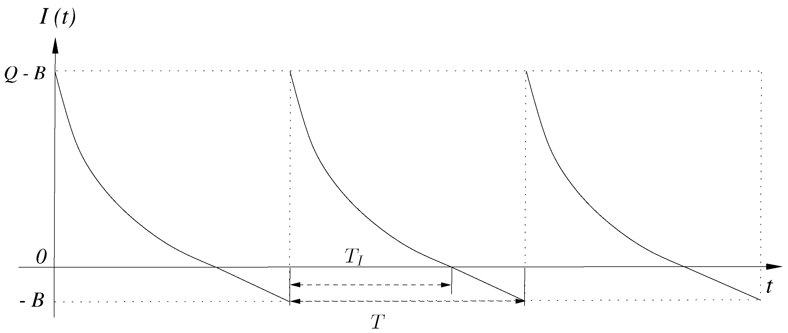
5. The Planned Backorders Model

Backordering satisfies the customer’s demand late when the item is out of stock and the customer is willing to wait, at the expense of a backordering cost per unit of the item. When the customer is willing to wait, it is always optimal to backorder a portion of the demand, as long as the per unit backordering cost is reasonably small. The backordering model is the general case of the basic model; it reduces to the basic model when the per unit cost of backordering approaches infinity. It is important to study it in addition to the basic model because it is a generalization of it. On the contrary, lost sales occur when the item is out of stock and the customer isn’t willing to wait. In this case, for deterministic demand, it is optimal to never allow lost sales, which means using the basic model [45].

B is the amount of demand left unfilled in a given cycle to be satisfied in the next cycle (i.e., backordered demand), and b is the cost of backordering per unit per unit time. Each cycle starts with a backorder amount of B units, which is immediately fulfilled from the received order. Thus, in the planned backorders model, the order quantity is Q, but the maximum inventory level is $Q-B$ (See Figure 2). This changes the inventory level and order quantity equations, as well as the waste cost per cycle and the inventory holding cost per cycle as follows:

$$\begin{array}{cc}\hfill I\left(t\right)& \hfill =(Q-B)e^{-\delta t}-\frac{D}{\delta }(1-e^{-\delta t}),0\le t\le T_I\hfill \end{array}$$

(51)

$$\begin{array}{cc}\hfill Q& \hfill =\frac{D}{\delta }(e^{\delta T_I}-1)+B\hfill \end{array}$$

(52)

$$\begin{array}{cc}\hfill B& \hfill =D(T-T_I)\hfill \end{array}$$

(53)

$$\begin{array}{cc}\hfill T_I& \hfill =\frac{1}{\delta }ln\left[\frac{D+\delta (Q-B)}{D}\right]\hfill \end{array}$$

(54)

$$\begin{array}{cc}\hfill W_c& \hfill =c(Q-B-D{T}_I)\hfill \end{array}$$

(55)

$$\begin{array}{cc}\hfill I_c& \hfill =\frac{h}{\delta }(Q-B-D{T}_I)\hfill \end{array}$$

(56)

where $T_I\le T$ is the length of time when the inventory level is non-zero during a cycle. It should be noted that $I\left(t\right)$ represents the on-hand inventory level and it is never negative. In Figure 2, the part of the graph below zero represents accumulating backorders, it does not represent negative on-hand inventory. Then, the exact unit time total cost for the deteriorating items with planned backorders model will be as follows:

$$\begin{array}{cc}\hfill & \hfill TC(T,T_I)=\frac{S}{T}+\frac{h+c\delta }{\delta T}\left[\frac{D}{\delta }(e^{\delta T_I}-1)-D{T}_I\right]+\frac{bD{(T-T_I)}^2}{2T}\hfill \end{array}$$

(57)

Lemma 3.

$TC(T,T_I)$ in Equation (57) is convex over $(T,T_I)\ge 0$.

Proof. 

The first term of $TC(T,T_I)$ in Equation (57) is obviously strictly convex. The second term can be rearranged as follows:

$$\begin{array}{c}\hfill \frac{(h+c\delta )D}{{\delta }^2}\left[\frac{e^{\delta T_I}-\delta T_I-1}{T}\right]=\frac{(h+c\delta )D}{{\delta }^2}f(T,T_I)\end{array}$$

(58)

The Hessian of $f(T,T_I)$ is as follows:

$$\begin{array}{c}\hfill H_f(T,T_I)=\left[\begin{array}{cc}{f}_{TT}& f_{T{T}_I}\\ f_{T_{I}T}& f_{T_I{T}_I}\end{array}\right]=\left[\begin{array}{cc}\frac{2(e^{\delta T_I}-\delta T_I-1)}{T^3}& -\frac{\delta }{T^2}(e^{\delta T_I}-1)\\ -\frac{\delta }{T^2}(e^{\delta T_I}-1)& \frac{{\delta }^2{e}^{\delta T_I}}{T}\end{array}\right]\end{array}$$

(59)

$f_{TT}\ge 0$ and $f_{T{T}_I}=f_{T_{I}T}<0$ for $(T,T_I)\ge 0$ because $e^{\delta T_I}=1+\delta T_I+\frac{{\delta }^2{T}^2}{2}+\dots$, due to Taylor series expansion. $f_{T_I{T}_I}>0$ for $(T,T_I)\ge 0$. The determinant of the leading principal minor is $f_{TT}\ge 0$. Furthermore, the other principal minor, $f_{T_I{T}_I}>0$. $f_{TT}=0$ if and only if $T_I=0$, in which case $f_{T{T}_I}=0$ as well. Using the Taylor series expansion of $e^{\delta T}$ again, $det\left(H_f(T,T_I)\right)\ge 0$ reduces to the following inequality that obviously holds:

$$\begin{array}{cc}\hfill & \hfill \frac{{\left(\delta T_I\right)}^3}{3}+\frac{{\left(\delta T_I\right)}^4}{3}+\frac{11{\left(\delta T_I\right)}^5}{60}+\dots +\frac{(2^n-2n){\left(\delta T_I\right)}^n}{n!}+\dots \ge 0\hfill \end{array}$$

(60)

The Hessian $H_g(T,T_I)$ of the third term of Equation (57) should satisfy the following inequality to be positive semi-definite:

$$\begin{array}{c}\hfill \left[\begin{array}{cc}x& y\end{array}\right]\left[\begin{array}{cc}\frac{2T_I^2}{T^3}& -\frac{2T_I}{T^2}\\ -\frac{2T_I}{T^2}& \frac{2}{T}\end{array}\right]\left[\begin{array}{c}x\\ y\end{array}\right]=\frac{2T_I^2}{T^3}{x}^2-\frac{4T_I}{T^2}xy+\frac{2}{T}{y}^2\ge 0,x,y\in \mathcal{R}\end{array}$$

(61)

Equation (61) holds because for a fixed y, ${\Delta }_x=y^2(\frac{16T_I^2}{T^4}-\frac{16T_I^2}{T^4})=0$ and $\frac{2T_I^2}{T^3}\ge 0$. If $\frac{2T_I^2}{T^3}=0$, Equation (61) holds for any x and y. Similarly, for a fixed x, ${\Delta }_y=x^2(\frac{16T_I^2}{T^4}-\frac{16T_I^2}{T^4})=0$ and $\frac{2}{T}>0$. □

We can alternatively express the total cost function in terms of Q and B as follows:

$$\begin{array}{cc}\hfill TC(Q,B)=& \hfill \frac{\delta S}{lnx+\delta \frac{B}{D}}+\frac{h+c\delta }{lnx+\delta \frac{B}{D}}\left[Q-B-\frac{D}{\delta }lnx\right]+\frac{\delta b{B}^2}{2D\left(lnx+\delta \frac{B}{D}\right)}\hfill \end{array}$$

(62)

where $x=1+\frac{\delta (Q-B)}{D}$. It can be similarly shown that Equation (62) also has a unique minimum. Like in the basic model, there is no exact closed-form equation in the planned backorders model for $T^{*}$ and $T_I^{*}$($Q^{*}$ and $B^{*}$) due to exponential (logarithmic) terms in Equation (57) (Equation (62)). Therefore, we propose approximations of the total cost function that are close and result in intuitive closed-form solutions.

5.1. Existing Closed-Form Solutions

Widyadana et al. [36] develop the following equations based on the same approximation as in their basic model:

$$\begin{array}{cc}\hfill Q^{*}& \hfill =\sqrt{\frac{2SD(D+\delta )}{[h{r}^2+b{(1-r)}^2][D+\delta (1-r)]}}\hfill \end{array}$$

(63)

$$\begin{array}{cc}\hfill B^{*}& \hfill =\left(\frac{b}{b+h}\right)Q^{*}\hfill \end{array}$$

(64)

where $r=\frac{b}{b+h}$ is the optimal “fill rate”, which is the fraction of the cycle demand that is immediately satisfied from the available inventory. Obviously, this optimal order quantity equation is far from being intuitive. In Section 6, we will show that it is also far from being accurate. Substituting $r=\frac{b}{b+h}$ in Equation (63), we obtain the following, which is still not intuitive (the last square root term is dubious):

$$\begin{array}{cc}\hfill Q^{*}& \hfill =\sqrt{\frac{2S(D+\delta )}{h}}\sqrt{\frac{b+h}{b}}\sqrt{\frac{D(b+h)}{D(b+h)+h\delta }}\hfill \end{array}$$

(65)

5.2. New Closed-Form Solutions

In this section, we develop new approximations of the total cost function similar to the basic model and derive closed-form equations for the optimal solution of the planned backorders model.

5.2.1. Closed-Form Solution 1

By once again substituting the Taylor series expansion of $e^{\delta T_I}=1+\delta T_I+\frac{{\delta }^2{T}_I^2}{2}$ in Equation (57), we obtain the following total cost function:

$$\begin{array}{c}\hfill TC(T,T_I)=\frac{S}{T}+\frac{(h+c\delta )D{T}_I^2}{2T}+\frac{bD{(T-T_I)}^2}{2T}\end{array}$$

(66)

Equation (66) is the same as the approximate total cost function in Çalışkan [24], who derives and optimizes it without using differential calculus.

Lemma 4.

$TC(T,T_I)$ in Equation (66) is convex over $(T,T_I)\ge 0$.

Proof. 

The Hessian of $TC(T,T_I)$ is as follows:

$$\begin{array}{c}\hfill H_{TC}(T,T_I)=\left[\begin{array}{cc}T{C}_{TT}& T{C}_{T{T}_I}\\ T{C}_{T_{I}T}& T{C}_{T_I{T}_I}\end{array}\right]=\left[\begin{array}{cc}\frac{2S}{T^3}+\frac{(h+c\delta +b)D{T}_I^2}{T^3}& -\frac{(h+c\delta +b)D{T}_I}{T^2}\\ -\frac{(h+c\delta +b)D{T}_I}{T^2}& \frac{(h+c\delta +b)D}{T}\end{array}\right]\end{array}$$

(67)

$T{C}_{TT}>0$ and $T{C}_{T{T}_I}=T{C}_{T_{I}T}\le 0$ for $(T,T_I)\ge 0$. $T{C}_{T_I{T}_I}>0$ for $(T,T_I)\ge 0$. The determinant of the leading principal minor is $T{C}_{TT}>0$. Furthermore, the other principal minor, $T{C}_{T_I{T}_I}>0$. Finally, $det\left(H_{TC}(T,T_I)\right)=\frac{2(h+c\delta +b)SD}{T^4}>0$. □

The Optimal Inventory Interval ($T_I$)

Setting $T{C}_{T_I}$ equal to zero yields the following equation for $T_I^{*}$:

$$\begin{array}{cc}\hfill & \hfill T_I^{*}=\left(\frac{b}{b+h+c\delta }\right)T^{*}\hfill \end{array}$$

(68)

The Optimal Order Interval (T)

We can eliminate $T_I$ from Equation (66) by substituting Equation (68) in Equation (66). The resulting total cost equation is as follows:

$$\begin{array}{c}\hfill TC\left(T\right)=\frac{S}{T}+\left[\frac{(h+c\delta )b}{b+h+c\delta }\right]\frac{DT}{2}\end{array}$$

(69)

Equation (69) has the same form as Equation (36). Therefore, the optimal order interval can be determined as follows:

$$\begin{array}{cc}\hfill T^{*}& \hfill =\sqrt{\frac{2S}{(h+c\delta )D}}\sqrt{\frac{b+h+c\delta }{b}}\hfill \end{array}$$

(70)

The optimal order and backorder quantities $(Q^{*},B^{*})$ can then be calculated using Equations (52) and (53).

5.2.2. Closed-Form Solution 2

We now consider Equation (62) and use the Taylor series expansion of $ln(1+x)=x-\frac{x^2}{2}+\frac{x^3}{3}-\frac{x^4}{4}+\dots$ with $x=\frac{\delta (Q-B)}{D}$. Because $\delta$ is usually small in practice, and $Q-B$ is usually much smaller than D for the optimal solution, we will ignore the terms higher than the second order. By substituting this approximation in Equation (62), we obtain:

$$\begin{array}{cc}\hfill TC(Q,B)=& \hfill \frac{1}{\frac{\delta Q}{D}-\frac{{\delta }^2{(Q-B)}^2}{2D^2}}\left(\delta S+(h+c\delta )\left[\frac{\delta {(Q-B)}^2}{2D}\right]+\frac{\delta b{B}^2}{2D}\right)\hfill \end{array}$$

(71)

In Equation (71), we can further ignore the quadratic term in the denominator because, in practice, $2D^2\gg \delta {(Q-B)}^2$, especially around the optimal solution. This results in the following total cost function:

$$\begin{array}{c}\hfill TC(Q,B)=\frac{SD}{Q}+\frac{(h+c\delta ){(Q-B)}^2}{2Q}+\frac{b{B}^2}{2Q}\end{array}$$

(72)

$TC(Q,B)$ in Equation (72) can be shown to be convex similar to how we prove the convexity of Equation (66).

The Optimal Backorder Quantity (B)

Setting $T{C}_B$ equal to zero yields the following equation for $B^{*}$:

$$\begin{array}{cc}\hfill & \hfill B^{*}=\left(\frac{h+c\delta }{b+h+c\delta }\right)Q^{*}\hfill \end{array}$$

(73)

The Optimal Order Quantity (Q)

We can eliminate B from Equation (72) by substituting Equation (73) in Equation (72). The resulting total cost function is as follows:

$$\begin{array}{c}\hfill TC\left(Q\right)=\frac{SD}{Q}+\left[\frac{(h+c\delta )b}{b+h+c\delta }\right]\frac{Q}{2}\end{array}$$

(74)

Equation (74) has the same form as Equation (41), except for the constant term. Therefore, the optimal order quantity can be determined as follows:

$$\begin{array}{cc}\hfill Q^{*}& \hfill =\sqrt{\frac{2DS}{h+c\delta }}\sqrt{\frac{b+h+c\delta }{b}}\hfill \end{array}$$

(75)

5.2.3. Closed-Form Solution 3

Closed-Form Solutions 1 and 2 can be hybridized to obtain a better approximate solution. Solution 1 results in an order quantity higher than the actual optimal order quantity, whereas Solution 2 results in an order quatity lower than the optimal order quantity. Let $T_{I_1}^{*}$, $T_1^{*}$ be the optimal inventory and order intervals from Solution 1, and let ($Q_2^{*},B_2^{*}$) be the optimal order and backorder quantities from Solution 2. Then, the following solution lies in between the two solutions:

$$\begin{array}{cc}\hfill Q^{*}& \hfill =\frac{1}{2}\left[\frac{D}{\delta }\left(e^{\delta T_{I_1}^{*}}-1\right)+D(T_1^{*}-T_{I_1}^{*})+Q_2^{*}\right].\hfill \end{array}$$

(76)

Then, $B^{*}$ can be calculated using Equation (73).

5.2.4. Closed-Form Solution 4

We can also hybridize Solutions 1 and 2 from the (T, $T_I$) side as well. This results in the following optimal solution:

$$\begin{array}{cc}\hfill T_I^{*}& \hfill =\frac{1}{2}\left[T_{I_1}^{*}+\frac{1}{\delta }ln\left(1+\frac{\delta (Q_2^{*}-B_2^{*})}{D}\right)\right].\hfill \end{array}$$

(77)

$T^{*}$ can then be calculated using Equation (68).

6. Results

In this section, we test the accuracy of our proposed approximation models against the existing ones as well as the approximated numerical solution of the exact model. In order to find the exact optimal solutions, we use the generalized reduced gradient (GRG) solver by Frontline Systems. The GRG solver is based on the nonlinear optimization algorithm by Lasdon et al. [46]. In the experiments, we analyze the change in $Q^{*}$, $B^{*}$, and $TC(.)$ with respect to $\delta$, S, D, and h, where we use $c=10$.

6.1. The Basic Model

We summarize the results of the numerical experiments for the basic model in

Table 2. The optimal order quantity of the GRG algorithm and the existing and proposed closed-form solutions for the basic model.

				Optimal Order Quantity ${\mathit{Q}}^{*}$
Parameters				Existing Solutions				New Solutions
$\mathit{D}$	$\mathit{S}$	$\mathit{h}$	$\mathbf{\delta }$	GRG	E1	E2	E3	N1	N2	N3	N4	N5	N6
500	100	3.5	0.1	149.81	149.57	149.06	169.05	151.32	149.07	146.87	149.81	150.18	150.19
500	100	3.5	1.25	81.62	85.40	78.82	169.24	87.41	79.06	71.63	81.66	82.96	83.10
500	100	3.5	2.5	62.09	67.53	58.86	169.45	68.94	59.23	51.11	62.17	63.62	63.85
500	100	3.5	3.75	52.35	58.67	48.92	169.66	59.77	49.39	41.08	52.44	53.96	54.27
500	100	3.5	5	46.25	53.17	42.69	169.87	54.09	43.23	34.89	46.36	47.91	48.28
500	10	3.5	1	27.46	27.77	27.21	53.51	27.97	27.22	26.49	27.46	27.59	27.59
500	60	3.5	1	68.13	70.03	66.57	131.06	71.32	66.67	62.37	68.15	68.89	68.94
500	110	3.5	1	92.94	96.49	90.04	177.46	98.93	90.27	82.49	92.99	94.34	94.47
500	160	3.5	1	112.75	117.97	108.48	214.02	121.63	108.87	97.66	112.82	114.79	115.02
500	210	3.5	1	129.81	136.74	124.15	245.19	141.66	124.72	110.13	129.92	132.50	132.84
1000	50	3.5	5	44.76	47.89	43.08	169.45	48.26	43.23	38.81	44.79	45.57	45.66
2000	50	3.5	5	62.68	65.71	61.03	239.34	66.06	61.14	56.65	62.70	63.48	63.54
4500	50	3.5	5	93.26	96.21	91.64	358.77	96.55	91.71	87.16	93.27	94.05	94.09
9000	50	3.5	5	131.25	134.16	129.65	507.23	134.49	129.70	125.11	131.26	132.04	132.07
100,000	50	3.5	5	433.89	436.73	432.32	1690.35	437.04	432.34	427.69	433.90	434.67	434.68
10,000	50	0.3	1	313.20	316.35	311.56	1825.83	316.49	311.59	306.77	313.21	314.02	314.03
10,000	50	0.8	1	305.83	308.61	304.27	1118.09	308.97	304.29	299.70	305.83	306.61	306.62
10,000	50	2.5	1	284.17	286.06	282.82	632.49	286.88	282.84	278.87	284.18	284.84	284.85
10,000	50	5	1	259.31	260.43	258.18	447.24	261.56	258.20	254.89	259.31	259.87	259.87
10,000	50	7.5	1	240.00	240.68	239.03	365.17	241.93	239.05	236.21	240.00	240.47	240.48
				% Difference of${\mathit{Q}}^{*}$vs. GRG
Parameters				Existing Solutions				New Solutions
$\mathit{D}$	$\mathit{S}$	$\mathit{h}$	$\mathbf{\delta }$	GRG	E1	E2	E3	N1	N2	N3	N4	N5	N6
500	100	3.5	0.1	0.00	−0.16	−0.50	12.84	1.01	−0.49	−1.96	0.00	0.25	0.25
500	100	3.5	1.25	0.00	4.63	−3.43	107.35	7.09	−3.14	−12.24	0.05	1.64	1.81
500	100	3.5	2.5	0.00	8.76	−5.20	172.91	11.03	−4.61	−17.68	0.13	2.46	2.83
500	100	3.5	3.75	0.00	12.07	−6.55	224.09	14.17	−5.65	−21.53	0.17	3.08	3.67
500	100	3.5	5	0.00	14.96	−7.70	267.29	16.95	−6.53	−24.56	0.24	3.59	4.39
500	10	3.5	1	0.00	1.13	−0.91	94.87	1.86	−0.87	−3.53	0.00	0.47	0.47
500	60	3.5	1	0.00	2.79	−2.29	92.37	4.68	−2.14	−8.45	0.03	1.12	1.19
500	110	3.5	1	0.00	3.82	−3.12	90.94	6.45	−2.87	−11.24	0.05	1.51	1.65
500	160	3.5	1	0.00	4.63	−3.79	89.82	7.88	−3.44	−13.38	0.06	1.81	2.01
500	210	3.5	1	0.00	5.34	−4.36	88.88	9.13	−3.92	−15.16	0.08	2.07	2.33
1000	50	3.5	5	0.00	6.99	−3.75	278.57	7.82	−3.42	−-13.29	0.07	1.81	2.01
2000	50	3.5	5	0.00	4.83	−2.63	281.84	5.39	−2.46	−9.62	0.03	1.28	1.37
4500	50	3.5	5	0.00	3.16	−1.74	284.70	3.53	−1.66	−6.54	0.01	0.85	0.89
9000	50	3.5	5	0.00	2.22	−1.22	286.46	2.47	−1.18	−4.68	0.01	0.60	0.62
100,000	50	3.5	5	0.00	0.65	−0.36	289.58	0.73	−0.36	−1.43	0.00	0.18	0.18
10,000	50	0.3	1	0.00	1.01	−0.52	482.96	1.05	−0.51	−2.05	0.00	0.26	0.27
10,000	50	0.8	1	0.00	0.91	−0.51	265.59	1.03	−0.50	−2.00	0.00	0.26	0.26
10,000	50	2.5	1	0.00	0.67	−0.48	122.57	0.95	−0.47	−1.87	0.00	0.24	0.24
10,000	50	5	1	0.00	0.43	−0.44	72.47	0.87	−0.43	−1.70	0.00	0.22	0.22
10,000	50	7.5	1	0.00	0.28	−0.40	52.15	0.80	−0.40	−1.58	0.00	0.20	0.20

and

Table 3. The optimal total cost of the GRG algorithm and the existing and proposed closed-form solutions for the basic model.

				Optimal Total Cost $\mathit{T}\mathit{C}\left({\mathit{Q}}^{*}\right)$ or $\mathit{T}\mathit{C}\left({\mathit{T}}^{*}\right)$
Parameters				Existing Solutions				New Solutions
$\mathit{D}$	$\mathit{S}$	$\mathit{h}$	$\mathbf{\delta }$	GRG	E1	E2	E3	N1	N2	N3	N4	N5	N6
500	100	3.5	0.1	674.15	674.15	674.15	679.00	674.18	674.15	674.28	674.15	674.15	674.15
500	100	3.5	1.25	1305.93	1307.14	1306.65	1628.75	1308.72	1306.53	1316.13	1305.93	1306.08	1306.12
500	100	3.5	2.5	1769.62	1775.08	1771.84	2576.62	1778.08	1771.34	1799.27	1769.62	1770.08	1770.22
500	100	3.5	3.75	2146.32	2158.16	2150.54	3464.35	2162.33	2149.43	2200.74	2146.33	2147.16	2147.50
500	100	3.5	5	2474.27	2494.17	2480.90	4307.94	2499.36	2478.96	2557.50	2474.28	2475.55	2476.16
500	10	3.5	1	370.74	370.76	370.76	453.41	370.80	370.76	370.98	370.74	370.75	370.75
500	60	3.5	1	919.79	920.11	920.02	1108.11	920.68	919.99	923.16	919.79	919.84	919.85
500	110	3.5	1	1254.75	1255.55	1255.33	1499.45	1256.99	1255.24	1263.00	1254.75	1254.87	1254.90
500	160	3.5	1	1522.11	1523.52	1523.14	1808.10	1526.06	1522.96	1536.41	1522.11	1522.33	1522.38
500	210	3.5	1	1752.38	1754.49	1753.93	2071.55	1758.34	1753.63	1773.66	1752.38	1752.71	1752.80
1000	50	3.5	5	2394.92	2399.84	2396.51	4479.47	2401.05	2396.23	2417.11	2394.92	2395.26	2395.34
2000	50	3.5	5	3353.40	3356.87	3354.51	6436.92	3357.70	3354.36	3369.43	3353.40	3353.65	3353.69
4500	50	3.5	5	4989.27	4991.58	4990.00	9806.59	4992.13	4989.94	5000.15	4989.27	4989.44	4989.46
9000	50	3.5	5	7021.86	7023.49	7022.37	14,014.64	7023.88	7022.34	7029.64	7021.86	7021.98	7021.99
100,000	50	3.5	5	23,213.25	23,213.74	23,213.40	47,686.78	23,213.85	23,213.40	23,215.63	23,213.25	23,213.29	23,213.29
10,000	50	0.3	1	3225.99	3226.14	3226.03	9438.50	3226.16	3226.03	3226.67	3225.99	3226.00	3226.00
10,000	50	0.8	1	3302.96	3303.09	3303.00	6402.80	3303.13	3303.00	3303.63	3302.96	3302.97	3302.97
10,000	50	2.5	1	3552.16	3552.24	3552.20	4727.92	3552.32	3552.20	3552.78	3552.16	3552.17	3552.17
10,000	50	5	1	3889.61	3889.65	3889.65	4472.61	3889.76	3889.65	3890.18	3889.61	3889.62	3889.62
10,000	50	7.5	1	4199.93	4199.95	4199.97	4570.20	4200.07	4199.97	4200.46	4199.93	4199.94	4199.94
				% Difference of$\mathit{T}\mathit{C}\left({\mathit{Q}}^{*}\right)$or$\mathit{T}\mathit{C}\left({\mathit{T}}^{*}\right)$vs. GRG
Parameters				Existing Solutions				New Solutions
$\mathit{D}$	$\mathit{S}$	$\mathit{h}$	$\mathbf{\delta }$	GRG	E1	E2	E3	N1	N2	N3	N4	N5	N6
500	100	3.5	0.1	0.00	0.00	0.00	0.72	0.00	0.00	0.02	0.00	0.00	0.00
500	100	3.5	1.25	0.00	0.09	0.06	24.72	0.21	0.05	0.78	0.00	0.01	0.01
500	100	3.5	2.5	0.00	0.31	0.13	45.60	0.48	0.10	1.68	0.00	0.03	0.03
500	100	3.5	3.75	0.00	0.55	0.20	61.41	0.75	0.14	2.54	0.00	0.04	0.05
500	100	3.5	5	0.00	0.80	0.27	74.11	1.01	0.19	3.36	0.00	0.05	0.08
500	10	3.5	1	0.00	0.01	0.00	22.30	0.02	0.00	0.06	0.00	0.00	0.00
500	60	3.5	1	0.00	0.04	0.03	20.47	0.10	0.02	0.37	0.00	0.01	0.01
500	110	3.5	1	0.00	0.06	0.05	19.50	0.18	0.04	0.66	0.00	0.01	0.01
500	160	3.5	1	0.00	0.09	0.07	18.79	0.26	0.06	0.94	0.00	0.01	0.02
500	210	3.5	1	0.00	0.12	0.09	18.21	0.34	0.07	1.21	0.00	0.02	0.02
1000	50	3.5	5	0.00	0.21	0.07	87.04	0.26	0.05	0.93	0.00	0.01	0.02
2000	50	3.5	5	0.00	0.10	0.03	91.95	0.13	0.03	0.48	0.00	0.01	0.01
4500	50	3.5	5	0.00	0.05	0.01	96.55	0.06	0.01	0.22	0.00	0.00	0.00
9000	50	3.5	5	0.00	0.02	0.01	99.59	0.03	0.01	0.11	0.00	0.00	0.00
100,000	50	3.5	5	0.00	0.00	0.00	105.43	0.00	0.00	0.01	0.00	0.00	0.00
10,000	50	0.3	1	0.00	0.00	0.00	192.58	0.01	0.00	0.02	0.00	0.00	0.00
10,000	50	0.8	1	0.00	0.00	0.00	93.85	0.01	0.00	0.02	0.00	0.00	0.00
10,000	50	2.5	1	0.00	0.00	0.00	33.10	0.00	0.00	0.02	0.00	0.00	0.00
10,000	50	5	1	0.00	0.00	0.00	14.99	0.00	0.00	0.01	0.00	0.00	0.00
10,000	50	7.5	1	0.00	0.00	0.00	8.82	0.00	0.00	0.01	0.00	0.00	0.00

, where the following is the notation to refer to different solutions:

GRG:	The exact optimal solution obtained by the GRG algorithm
E1:	The closed-form solution of Ghare and Schrader [9]
E2:	The closed-form solution of Chung and Ting [21]
E3:	The closed-form solution of Widyadana et al. [36]
Ni:	The proposed closed-form solution i in this paper where i = 1, 2, 3, 4, 5, 6

The $Q^{*}$ values in Table 2 for different models are determined using their respective closed-form solutions (and then using Equation (5) if the closed-form solution is used for $T^{*}$). The $TC\left(Q^{*}\right)$ values in Table 3 are calculated using Equations (4), (5) and (13). Among all closed-form solutions, Widyadana et al. [36] stands out as the most inaccurate. A closer look at Table 2 shows that for the Widyadana et al. [36] model, $Q^{*}$ is slightly increasing with $\delta$, but it should really decrease significantly. This is also apparent in Equation (34), which is an increasing function of $\delta$. If we compare $Q^{*}$ as it varies with respect to S, the solution introduced by Widyadana et al. [36] is approximately double the other solutions for every value of S; with respect to D, it is about seven to eight times the other solutions for every value of D; and with respect to h, it is about six times the others for a very small h and gradually becomes closer to others, but it is still 1.5 times the others, even for an h as large as $7.5$ (which corresponds to an inventory holding cost rate of 75%).

Closed-Form Solution 4 stands out as the most accurate one, which is almost identical to the exact solution in all of the cases. This is because it uses a more accurate approximation of $e^{\delta T}$ that includes the cubic term from the Taylor series expansion. Closed-Form Solutions 5 and 6, which are both hybrids of Solutions 1 and 2, are the next closest to the exact solution. This is due to Solutions 1 and 2 alternately overestimating and underestimating $Q^{*}$, so it is natural that their average would be closer to the exact solution. The solution of Chung and Ting [21] and Closed-Form Solution 2 are very close, because they both use the same approximation for $e^{\delta T}$. The difference is caused by the calculation of $Q^{*}$ from $T^{*}$ that uses the exact equation for $Q\left(T\right)$ (Equation (5)). They are similarly accurate, but our closed-form solution is much more intuitive than that of Chung and Ting [21].

The solution of Ghare and Schrader [9] and Closed-Form Solution 1 are also very close to one another, because they use the same approximation of $e^{\delta T}$. However, the latter is much more intuitive than the former. The difference in $Q^{*}$ and $TC\left(Q^{*}\right)$ is due to the fact that Ghare and Schrader [9] assume that the inventory holding cost is simply $hQ$ (which we use $h\frac{Q}{2}$ as in Chung and Ting [21] to avoid an unfair comparison), whereas Closed-Form Solution 1 is based on an exact integration-based modeling of the holding cost. This seemingly small issue leads to a depressed cubic equation in Ghare and Schrader [9] that fails to result in a simple and intuitive closed-form equation.

Finally, apart from Widyadana et al. [36], Closed-Form Solution 3 is the least accurate among all approaches, which is based on the Taylor series expansion of $ln(1+x)$. It might be more accurate if the third-order term is included, but then it does not lend itself to a simple closed-form solution. The closed-form solution with the present approximation is also not very intuitive, which is similar in its form to the closed-form equation of Chung and Ting [21], because they both come from the quadratic equation for the roots.

The conclusion for the basic model is that all of our closed-form solutions are reasonably accurate, and some of them (Equations (37), (42) and (48)) are very intuitive compared to the existing ones. Equation (48) is very accurate, almost identical to the exact optimal solution. Equations (37) and (42) are reasonably accurate in addition to being intuitive. Finally, the two hybrids, Equations (49) and (50), are very accurate as well. The closed-form solutions of Ghare and Schrader [9] and Chung and Ting [21] are reasonably accurate but not very intuitive, and Widyadana et al. [36] is somewhat intuitive but completely wrong.

6.2. The Planned Backorders Model

We summarize the results of the numerical experiments for the planned backorders model in

Table 4. The optimal order quantity and optimal backorder quantity of the GRG algorithm and the existing and proposed closed-form solutions for the planned backorders model.

					Optimal Order Quantity ${\mathit{Q}}^{*}$						Optimal Backorder Quantity ${\mathit{B}}^{*}$
Parameters					Existing		New Solutions				Existing		New Solutions
$\mathit{D}$	$\mathit{S}$	$\mathit{h}$	$\mathbf{\delta }$	$\mathit{b}$	GRG	E3	N1	N2	N3	N4	GRG	E3	N1	N2	N3	N4
500	100	3.5	0.1	20	165.59	170.52	166.82	164.99	165.91	165.91	30.42	25.40	30.30	30.30	30.30	30.47
500	100	3.5	1.25	20	107.46	170.68	110.63	106.07	108.35	108.34	47.76	25.42	47.14	47.14	47.14	48.15
500	100	3.5	2.5	20	93.38	170.86	96.10	92.24	94.17	94.16	54.87	25.45	54.20	54.20	54.20	55.33
500	100	3.5	3.75	20	87.18	171.03	89.47	86.25	87.86	87.85	58.60	25.47	57.97	57.97	57.97	59.05
500	100	3.5	5	20	83.66	171.21	85.63	82.88	84.25	84.25	60.90	25.50	60.33	60.33	60.33	61.32
500	10	3.5	1	20	35.37	53.96	35.67	35.22	35.45	35.45	14.25	8.04	14.19	14.19	14.19	14.29
500	60	3.5	1	20	87.14	132.18	89.03	86.28	87.65	87.65	35.12	19.69	34.77	34.77	34.77	35.32
500	110	3.5	1	20	118.39	178.97	121.92	116.83	119.37	119.37	47.71	26.66	47.08	47.08	47.08	48.10
500	160	3.5	1	20	143.16	215.85	148.39	140.90	144.64	144.63	57.69	32.15	56.78	56.78	56.78	58.28
500	210	3.5	1	20	164.37	247.29	171.33	161.42	166.37	166.35	66.24	36.83	65.05	65.05	65.05	67.04
1000	50	3.5	5	500	46.86	169.51	50.01	45.49	47.75	47.74	4.53	1.18	4.40	4.40	4.40	4.40
2000	50	3.5	5	500	65.71	239.43	68.76	64.33	66.55	66.54	6.35	1.66	6.22	6.22	6.22	6.22
4500	50	3.5	5	500	97.88	358.89	100.86	96.49	98.68	98.67	9.46	2.49	9.33	9.33	9.33	9.33
9000	50	3.5	5	500	137.86	507.41	140.78	136.46	138.62	138.62	13.33	3.53	13.19	13.19	13.19	13.19
100,000	50	3.5	5	500	456.28	1690.94	459.13	454.88	457.01	457.01	44.10	11.75	43.97	43.97	43.97	43.97
10,000	50	0.3	1	20	384.58	1827.20	386.75	383.52	385.14	385.14	130.73	27.00	130.37	130.37	130.37	130.92
10,000	50	0.8	1	20	378.61	1120.32	380.65	377.61	379.13	379.13	132.76	43.09	132.41	132.41	132.41	132.94
10,000	50	2.5	1	20	361.37	636.42	363.03	360.56	361.80	361.79	138.99	70.71	138.68	138.68	138.68	139.15
10,000	50	5	1	20	342.20	452.79	343.48	341.57	342.52	342.52	146.66	90.56	146.39	146.39	146.39	146.80
10,000	50	7.5	1	20	327.83	371.94	328.86	327.33	328.09	328.09	152.99	101.44	152.75	152.75	152.75	153.11
					% Difference of${\mathit{Q}}^{*}$and${\mathit{B}}^{*}$vs. GRG
					Optimal Order Quantity${\mathit{Q}}^{*}$						Optimal Backorder Quantity${\mathit{B}}^{*}$
Parameters					Existing		New Solutions				Existing		New Solutions
$\mathit{D}$	$\mathit{S}$	$\mathit{h}$	$\mathbf{\delta }$	$\mathit{b}$	GRG	E3	N1	N2	N3	N4	GRG	E3	N1	N2	N3	N4
500	100	3.5	0.1	20	0.00	2.98	0.74	−0.36	0.19	0.19	0.00	−16.50	−0.39	−0.39	−0.39	0.16
500	100	3.5	1.25	20	0.00	58.83	2.95	−1.29	0.83	0.82	0.00	−46.78	−1.30	−1.30	−1.30	0.82
500	100	3.5	2.5	20	0.00	82.97	2.91	−1.22	0.85	0.84	0.00	−53.62	−1.22	−1.22	−1.22	0.84
500	100	3.5	3.75	20	0.00	96.18	2.63	−1.07	0.78	0.77	0.00	−56.54	−1.08	−1.08	−1.08	0.77
500	100	3.5	5	20	0.00	104.65	2.35	−0.93	0.71	0.71	0.00	−58.13	−0.94	−0.94	−0.94	0.69
500	10	3.5	1	20	0.00	52.56	0.85	−0.42	0.23	0.23	0.00	−43.58	−0.42	−0.42	−0.42	0.28
500	60	3.5	1	20	0.00	51.69	2.17	−0.99	0.59	0.59	0.00	−43.94	−1.00	−1.00	−1.00	0.57
500	110	3.5	1	20	0.00	51.17	2.98	−1.32	0.83	0.83	0.00	−44.12	−1.32	−1.32	−1.32	0.82
500	160	3.5	1	20	0.00	50.78	3.65	−1.58	1.03	1.03	0.00	−44.27	−1.58	−1.58	−1.58	1.02
500	210	3.5	1	20	0.00	50.45	4.23	−1.79	1.22	1.20	0.00	−44.40	−1.80	−1.80	−1.80	1.21
1000	50	3.5	5	500	0.00	261.74	6.72	−2.92	1.90	1.88	0.00	−73.95	−2.87	−2.87	−2.87	−2.87
2000	50	3.5	5	500	0.00	264.37	4.64	−2.10	1.28	1.26	0.00	−73.86	−2.05	−2.05	−2.05	−2.05
4500	50	3.5	5	500	0.00	266.66	3.04	−1.42	0.82	0.81	0.00	−73.68	−1.37	−1.37	−1.37	−1.37
9000	50	3.5	5	500	0.00	268.06	2.12	−1.02	0.55	0.55	0.00	−73.52	−1.05	−1.05	−1.05	−1.05
100,000	50	3.5	5	500	0.00	270.59	0.62	−0.31	0.16	0.16	0.00	−73.36	−0.29	−0.29	−0.29	−0.29
10,000	50	0.3	1	20	0.00	375.12	0.56	−0.28	0.15	0.15	0.00	−79.35	−0.28	−0.28	−0.28	0.15
10,000	50	0.8	1	20	0.00	195.90	0.54	−0.26	0.14	0.14	0.00	−67.54	−0.26	−0.26	−0.26	0.14
10,000	50	2.5	1	20	0.00	76.11	0.46	−0.22	0.12	0.12	0.00	−49.13	−0.22	−0.22	−0.22	0.12
10,000	50	5	1	20	0.00	32.32	0.37	−0.18	0.09	0.09	0.00	−38.25	−0.18	−0.18	−0.18	0.10
10,000	50	7.5	1	20	0.00	13.46	0.31	−0.15	0.08	0.08	0.00	−33.70	−0.16	−0.16	−0.16	0.08

and

Table 5. The optimal total cost of the GRG algorithm and the existing and proposed closed-form solutions for the planned backorders model.

					Optimal Total Cost $\mathit{T}\mathit{C}({\mathit{Q}}^{*},{\mathit{B}}^{*})$ or $\mathit{T}\mathit{C}(\mathit{T},{\mathit{T}}_{\mathit{I}})$
Parameters					Existing		New Solutions
$\mathit{D}$	$\mathit{S}$	$\mathit{h}$	$\mathbf{\delta }$	$\mathit{b}$	GRG	E3	N1	N2	N3	N4
500	100	3.5	0.1	20	608.30	611.08	608.33	608.31	608.30	608.31
500	100	3.5	1.25	20	955.18	1292.64	956.16	955.26	955.22	955.37
500	100	3.5	2.5	20	1097.44	1947.59	1098.96	1097.52	1097.48	1097.77
500	100	3.5	3.75	20	1171.91	2537.43	1173.60	1171.98	1171.95	1172.29
500	100	3.5	5	20	1217.92	3077.12	1219.63	1217.98	1217.95	1218.32
500	10	3.5	1	20	285.07	366.85	285.10	285.07	285.08	285.08
500	60	3.5	1	20	702.35	894.07	702.72	702.38	702.42	702.42
500	110	3.5	1	20	954.21	1207.62	955.11	954.29	954.38	954.38
500	160	3.5	1	20	1153.83	1454.04	1155.42	1153.97	1154.13	1154.13
500	210	3.5	1	20	1324.79	1663.74	1327.18	1324.99	1325.24	1325.24
1000	50	3.5	5	500	2264.74	4417.00	2270.03	2265.66	2265.36	2265.35
2000	50	3.5	5	500	3175.80	6350.39	3179.53	3176.48	3176.22	3176.22
4500	50	3.5	5	500	4730.68	9678.66	4733.15	4731.14	4730.95	4730.94
9000	50	3.5	5	500	6662.58	13,835.06	6664.33	6662.92	6662.76	6662.76
100,000	50	3.5	5	500	22,051.65	47,093.84	22,052.17	22,051.75	22,051.70	22,051.70
10,000	50	0.3	1	20	2614.65	9172.20	2614.74	2614.66	2614.66	2614.66
10,000	50	0.8	1	20	2655.19	5973.18	2655.28	2655.20	2655.21	2655.21
10,000	50	2.5	1	20	2779.78	3990.02	2779.85	2779.79	2779.79	2779.79
10,000	50	5	1	20	2933.11	3456.57	2933.17	2933.12	2933.12	2933.12
10,000	50	7.5	1	20	3059.77	3344.22	3059.81	3059.77	3059.78	3059.78
					% Difference of$\mathit{T}\mathit{C}({\mathit{Q}}^{*},{\mathit{B}}^{*})$or$\mathit{T}\mathit{C}(\mathit{T},{\mathit{T}}_{\mathit{I}})$vs. GRG
Parameters					Existing		New Solutions
$\mathit{D}$	$\mathit{S}$	$\mathit{h}$	$\mathbf{\delta }$	$\mathit{b}$	GRG	E3	N1	N2	N3	N4
500	100	3.5	0.1	20	0.00	0.46	0.00	0.00	0.00	0.00
500	100	3.5	1.25	20	0.00	35.33	0.10	0.01	0.00	0.02
500	100	3.5	2.5	20	0.00	77.47	0.14	0.01	0.00	0.03
500	100	3.5	3.75	20	0.00	116.52	0.14	0.01	0.00	0.03
500	100	3.5	5	20	0.00	152.65	0.14	0.00	0.00	0.03
500	10	3.5	1	20	0.00	28.69	0.01	0.00	0.00	0.00
500	60	3.5	1	20	0.00	27.30	0.05	0.00	0.01	0.01
500	110	3.5	1	20	0.00	26.56	0.10	0.01	0.02	0.02
500	160	3.5	1	20	0.00	26.02	0.14	0.01	0.03	0.03
500	210	3.5	1	20	0.00	25.59	0.18	0.02	0.03	0.03
1000	50	3.5	5	500	0.00	95.03	0.23	0.04	0.03	0.03
2000	50	3.5	5	500	0.00	99.96	0.12	0.02	0.01	0.01
4500	50	3.5	5	500	0.00	104.59	0.05	0.01	0.01	0.01
9000	50	3.5	5	500	0.00	107.65	0.03	0.01	0.00	0.00
100,000	50	3.5	5	500	0.00	113.56	0.00	0.00	0.00	0.00
10,000	50	0.3	1	20	0.00	250.80	0.00	0.00	0.00	0.00
10,000	50	0.8	1	20	0.00	124.96	0.00	0.00	0.00	0.00
10,000	50	2.5	1	20	0.00	43.54	0.00	0.00	0.00	0.00
10,000	50	5	1	20	0.00	17.85	0.00	0.00	0.00	0.00
10,000	50	7.5	1	20	0.00	9.30	0.00	0.00	0.00	0.00

, where the following is the notation to refer to different solutions:

GRG:	The exact optimal solution obtained by the GRG algorithm
E3:	The closed-form solution of Widyadana et al. [36]
Ni:	The proposed closed-form solution i in this paper where i = 1, 2, 3, 4

The $Q^{*}$ and $B^{*}$ values in Table 4 for different models are determined using their respective closed-form solutions (and then using Equation (52) and (53) if the closed-form solution is used for $T_I^{*}$ and $T^{*}$). The $TC(Q^{*},B^{*})$ values in Table 5 are calculated using Equations (52)–(54), and (57). Widyadana et al. [36] again stands out as the most inaccurate.

As it is shown in Table 4 and Table 5, both Closed-Form Solution 1 and Closed-Form Solution 2 are very close to optimal values. One of them is above and the other is below as in the basic model (in terms of $Q^{*}$ and $B^{*}$). Hybrid solutions (Closed-Form Solutions 3 and 4) are almost identical to one another and they are closest to the exact optimum solution. In terms of total cost, they are almost identical to the exact total cost in all cases. Closed-Form Solutions 1 and 2 are almost identical in terms of total cost, and they are not very far from the optimal cost, either.

Keeping all parameters constant but varying S produces the biggest difference between the different models in terms of $Q^{*}$, especially as S becomes larger. However, when we look at $B^{*}$ and $TC(Q^{*},B^{*})$, the differences are much smaller. The next greatest difference happens with respect to $\delta$. For varying D, differences are much smaller and they almost disappear as it becomes larger. Finally, for varying h, differences are much smaller and they do not change much between small or large values of h.

We do not include experiments for varying b, but our experience is that all closed-form solutions approach their counterpart basic model as b becomes larger. This is apparent from the factors $\frac{b+h+c\delta }{b}$ and $\frac{b}{b+h+c\delta }$ that appear in both of our closed-form solutions and $\frac{b+h}{b}$ and $\frac{b}{b+h}$ in the Widyadana et al. [36] model, as they all approach 1 as $b\to \infty$.

In summary, we can confidently assert that all of our closed-form solutions for the planned backorders model are quite accurate and very intuitive. Widyadana et al. [36] propose the earliest solution in the literature for the exponentially deteriorating items model with planned backorders. However, it is not only most inaccurate and counterintuitive, but also incorrect as the model behaves opposite to the exact model for some of the parameters such as $\delta$.

7. Conclusions

In this research, we propose six different closed-form solutions for the basic exponentially deteriorating items inventory model and four different closed-form solutions for the planned backorders version of the same model. Our closed-form equations are based on the novel use of Taylor series approximations of the exponential and logarithmic functions. Some of these approximations have been previously used for this problem but, due to modelling choices of the previous researchers, they have not been able to develop intuitive closed-form solutions. Our contribution is that we propose intuitive closed-form solutions that are quite useful for the practitioners and we show that they are very accurate as well. We provide complete proofs to show that the proposed closed-form solutions are unique optimal solutions, which is another contribution of our research.

8. Limitations and Future Research

In this research, we assume that the demand is constant and deterministic. In practice, demand may be price- or time-dependent in some cases. Future research may consider price- and/or time-dependent demand functions. Exponentially increasing or exponentially decreasing demand can also be studied. We also assume that the purchase and ordering costs are paid at the time of order delivery. In practice, there may be a variety of payment structures that extend credit to the retailer. Future research may consider extending our models to trade credit scenarios. Finally, we assume constant deterioration in this research, where the time to deterioration for individual items follow an exponential distribution; hence, it is also called exponential deterioration. Exponential distribution has memoryless property, which means that the probability of deterioration is independent of the lifetime that has already elapsed. This makes the instantaneous deterioration rate constant, which is why it is called constant deterioration. In practice, for some items, the probability of deterioration may become higher as the elapsed lifetime becomes longer. Future research may consider different deterioration distributions that allow variable deterioration rates.

References

1. Kaur, J.; Rani, G.; Yogalakshmi, K. Chapter 16—Problems and Issues of Food Waste-Based Biorefineries. In Food Waste to Valuable Resources; Banu, J.R., Kumar, G., Gunasekaran, M., Kavitha, S., Eds.; Academic Press: Cambridge, MA, USA, 2020; pp. 343–357. [Google Scholar]
2. Huang, C.H.; Liu, S.M.; Hsu, N.Y. Understanding Global Food Surplus and Food Waste to Tackle Economic and Environmental Sustainability. Sustainability 2020, 12, 2892. [Google Scholar] [CrossRef] [Green Version]
3. Zamri, G.B.; Azizal, N.K.A.; Nakamura, S.; Okada, K.; Nordin, N.H.; Othman, N.; MD Akhir, F.N.; Sobian, A.; Kaida, N.; Hara, H. Delivery, impact and approach of household food waste reduction campaigns. J. Clean. Prod. 2020, 246, 118969. [Google Scholar] [CrossRef]
4. Moraes, N.V.; Lermen, F.H.; Echeveste, M.E.S. A systematic literature review on food waste/loss prevention and minimization methods. J. Environ. Manag. 2021, 286, 112268. [Google Scholar] [CrossRef]
5. Gustavsson, J.; Cederberg, C.; Sonesson, U.; van Otterdijk, R.; Meybeck, A. Global Food Losses and Food Waste—Extent, Causes and Prevention. In SAVE FOOD: An Initiative on Food Loss and Waste Reduction; Interpack2011, FAO, International Congress: Düsseldorf, Germany, 2011. [Google Scholar]
6. Silver, E.A.; Pyke, D.F.; Peterson, R. Inventory Management and Production Planning and Scheduling, 3rd ed.; Wiley: Hoboken, NJ, USA, 1998. [Google Scholar]
7. Erlenkotter, D. Ford Whitman Harris and the Economic Order Quantity Model. Oper. Res. 1990, 38, 937–946. [Google Scholar] [CrossRef] [Green Version]
8. Harris, F. How Many Parts to Make at Once. Fact. Mag. Manag. 1913, 10, 135–136, 152. [Google Scholar] [CrossRef]
9. Ghare, P.M.; Schrader, G.F. A Model for an Exponentially Decaying Inventory. J. Ind. Eng. 1963, 14, 238–243. [Google Scholar]
10. Çalışkan, C. A derivation of the optimal solution for exponentially deteriorating items without derivatives. Comput. Ind. Eng. 2020, 148, 106675. [Google Scholar] [CrossRef]
11. Nahmias, S. Perishable Inventory Theory: A Review. Oper. Res. 1982, 30, 680–708. [Google Scholar] [CrossRef]
12. Raafat, F. Survey of Literature on Continuously Deteriorating Inventory Models. J. Oper. Res. Soc. 1991, 42, 27–37. [Google Scholar] [CrossRef]
13. Goyal, S.; Giri, B. Recent trends in modeling of deteriorating inventory. Eur. J. Oper. Res. 2001, 134, 1–16. [Google Scholar] [CrossRef]
14. Li, R.; Lan, H.; Mawhinney, J.R. A Review on Deteriorating Inventory Study. J. Serv. Sci. Manag. 2010, 3, 117–129. [Google Scholar] [CrossRef] [Green Version]
15. Bakker, M.; Riezebos, J.; Teunter, R.H. Review of inventory systems with deterioration since 2001. Eur. J. Oper. Res. 2012, 221, 275–284. [Google Scholar] [CrossRef]
16. Elsayed, E.; Teresi, C. Analysis of inventory systems with deteriorating items. Int. J. Prod. Res. 1983, 21, 449–460. [Google Scholar] [CrossRef]
17. Schmidt, C.P.; Nahmias, S. (S-1,S) Policies for Perishable Inventory. Manag. Sci. 1985, 31, 719–728. [Google Scholar] [CrossRef]
18. Dave, U.; Patel, L.K. (T, Si) Policy Inventory Model for Deteriorating Items with Time Proportional Demand. J. Oper. Res. Soc. 1981, 32, 137–142. [Google Scholar] [CrossRef]
19. Bahari-Kashani, H. Replenishment Schedule for Deteriorating Items with Time-Proportional Demand. J. Oper. Res. Soc. 1989, 40, 75–81. [Google Scholar] [CrossRef]
20. Chung, K.J.; Ting, P.S. A Heuristic for Replenishment of Deteriorating Items with a Linear Trend in Demand. J. Oper. Res. Soc. 1993, 44, 1235–1241. [Google Scholar] [CrossRef]
21. Chung, K.J.; Ting, P.S. On replenishment schedule for deteriorating items with time-proportional demand. Prod. Plan. Control 1994, 5, 392–396. [Google Scholar] [CrossRef]
22. Kim, D. A heuristic for replenishment of deteriorating items with a linear trend in demand. Int. J. Prod. Econ. 1995, 39, 265–270. [Google Scholar] [CrossRef]
23. Çalışkan, C. A note about ‘on replenishment schedule for deteriorating items with time-proportional demand’. Prod. Plan. Control 2021, 32, 1158–1161. [Google Scholar] [CrossRef]
24. Çalışkan, C. EOQ Model for Exponentially Deteriorating Items with Planned Backorders without Differential Calculus. Am. J. Math. Manag. Sci. 2022, 41, 223–243. [Google Scholar] [CrossRef]
25. Sachan, R.S. On (T, Si) Policy Inventory Model for Deteriorating Items with Time Proportional Demand. J. Oper. Res. Soc. 1984, 35, 1013–1019. [Google Scholar] [CrossRef]
26. Wee, H.M. Economic production lot size model for deteriorating items with partial backordering. Comput. Ind. Eng. 1993, 24, 449–458. [Google Scholar] [CrossRef]
27. Wee, H.M. A deterministic lot-size inventory model for deteriorating items with shortages and a declining market. Comput. Oper. Res. 1995, 22, 345–356. [Google Scholar]
28. Hariga, M.; Benkherouf, L. Optimal and heuristic inventory replenishment models for deteriorating items with exponential time-varying demand. Eur. J. Oper. Res. 1994, 79, 123–137. [Google Scholar] [CrossRef]
29. Benkherouf, L. On an inventory model with deteriorating items and decreasing time-varying demand and shortages. Eur. J. Oper. Res. 1995, 86, 293–299. [Google Scholar] [CrossRef]
30. Benkherouf, L.; Mahmoud, M.G. On an Inventory Model for Deteriorating Items with Increasing Time-varying Demand and Shortages. J. Oper. Res. Soc. 1996, 47, 188–200. [Google Scholar] [CrossRef]
31. Balkhi, Z.T.; Benkherouf, L. A production lot size inventory model for deteriorating items and arbitrary production and demand rates. Eur. J. Oper. Res. 1996, 92, 302–309. [Google Scholar] [CrossRef]
32. Giri, B.; Jalan, A.; Chaudhuri, K. Economic Order Quantity model with Weibull deterioration distribution, shortage and ramp-type demand. Int. J. Syst. Sci. 2003, 34, 237–243. [Google Scholar] [CrossRef]
33. Chang, H.J.; Dye, C.Y. An EOQ model for deteriorating items with time varying demand and partial backlogging. J. Oper. Res. Soc. 1999, 50, 1176–1182. [Google Scholar] [CrossRef]
34. Wang, S.P. A note on Chang H-J and Dye C-Y (1999). An EOQ model for deteriorating items with time varying demand and partial backlogging. J. Oper. Res. Soc. 2001, 52, 597–598. [Google Scholar] [CrossRef]
35. Goyal, S.K.; Giri, B.C. A comment on Chang and Dye (1999): EOQ model for deteriorating items with time-varying demand and partial backlogging. J. Oper. Res. Soc. 2001, 52, 238–239. [Google Scholar] [CrossRef]
36. Widyadana, G.A.; Cárdenas-Barrón, L.E.; Wee, H.M. Economic order quantity model for deteriorating items with planned backorder level. Math. Comput. Model. 2011, 54, 1569–1575. [Google Scholar] [CrossRef]
37. Çalışkan, C. A Simple Derivation of the Optimal Solution for the EOQ Model for Deteriorating Items with Planned Backorders. Appl. Math. Model. 2021, 89, 1373–1381. [Google Scholar] [CrossRef]
38. Haijema, R. A new class of stock-level dependent ordering policies for perishables with a short maximum shelf life. Int. J. Prod. Econ. 2013, 143, 434–439. [Google Scholar] [CrossRef]
39. Mishra, V.K.; Singh, L.S.; Kumar, R. An inventory model for deteriorating items with time-dependent demand and time-varying holding cost under partial backlogging. J. Ind. Eng. Int. 2013, 9, 4. [Google Scholar] [CrossRef] [Green Version]
40. Mahajan, S.; Diatha, K. Minimizing the Discounted Average Cost Under Continuous Compounding in the EOQ Models with a Regular Product and a Perishable Product. Am. J. Oper. Manag. Inf. Syst. 2018, 3, 52–60. [Google Scholar] [CrossRef] [Green Version]
41. Çalışkan, C. An Inventory Ordering Model for Deteriorating Items with Compounding and Backordering. Symmetry 2021, 13, 1078. [Google Scholar] [CrossRef]
42. Shelbey, S. CRC Standard Mathematical Tables, 23rd ed.; CRC Press: Boca Raton, FL, USA, 1975. [Google Scholar]
43. Zucker, I. The cubic equation—A new look at the irreducible case. Math. Gaz. 2008, 92, 264–268. [Google Scholar] [CrossRef]
44. Nickalls, R. Viète, Descartes and the cubic equation. Math. Gaz. 2006, 90, 203–208. [Google Scholar] [CrossRef] [Green Version]
45. Zipkin, P.H. Foundations of Inventory Management, 1st ed.; McGraw-Hill: New York, NY, USA, 2000. [Google Scholar]
46. Lasdon, L.S.; Waren, A.D.; Jain, A.; Ratner, M. Design and Testing of a Generalized Reduced Gradient Code for Nonlinear Programming. ACM Trans. Math. Softw. 1978, 4, 34–50. [Google Scholar] [CrossRef]
Figure 1. Total Cost function for D = 1000, S = 50 , h = 3 , c = 10 and δ = 10 .
Sustainability 14 08389 g001
Figure 2. Inventory level over time in the planned backorders model.
Sustainability 14 08389 g002