Article

A Graphical Method for Designing the Horizontal Alignment and the Cant in High-Speed Railway Lines Aimed at Mixed-Speed Traffic

by
Ali Alqatawna
,
Santos Sánchez-Cambronero
*,
Inmaculada Gallego
and
Juan Miguel López-Morales
Department of Civil and Building Engineering, University of Castilla La Mancha, 13071 Ciudad Real, Spain
*
Author to whom correspondence should be addressed.
Sustainability 2022, 14(14), 8377; https://doi.org/10.3390/su14148377
Submission received: 9 June 2022 / Revised: 4 July 2022 / Accepted: 5 July 2022 / Published: 8 July 2022
(This article belongs to the Special Issue Sustainable Operation and Maintenance of Railway Systems)

Abstract

:
To realize the design of mixed-traffic railway lines, the choice of radius must ensure a comfortable ride for passenger vehicles, safe freight transport, and acceptable maintenance costs of vehicle wheels and railway infrastructure. This is not a straightforward task, and what is worse, there is a worldwide lack of clear criteria to limit the design parameters involved in the geometric definition of high-speed railway lines. The proof of this is the great number of technical standards (or recommendations) that are applied depending on the period of time, the administrations involved, or the technicians in charge. If the line is going to be aimed at mixed-speed traffic, this indetermination is even more severe, as the different type of trains that are forecasted to use the tracks (with different loads, speeds, etc.) should affect the limits of the design parameters. To begin to solve this problem, this paper aimed (1) to analyze the design parameters and limitation defined in several technical standards that are used to design high-speed railway lines, (2) to propose a graphical method for designing the horizontal alignment (the cant, the radius, and the clothoid), and (3) to apply the method to a real example to compare our proposed design with the original project for a case study in Spain.

1. Introduction and Motivation

Railways are one of the world’s most essential modes of transportation for both people and freight (see Watson et al. [1]), and particularly in the last two to three decades, high-speed railway lines have been developed all around the world. One interesting point is that the term “high-speed” in the railway context is related to the passenger market rather than freight transport. Therefore, high-speed trains are made for passengers, and high-speed railway lines cannot be used by freight trains (see, for example, Biancardo et al. [2]).
Rakoczy et al. [3] highlighted that as global commerce and corporate internationalization have increased, there has been a growing awareness of the need for more sustainable transportation, particularly for freight transit. This is mostly due to the connected concerns of greenhouse gas emissions and reliance on fossil fuels. The global growth of high-speed railway (HSR) lines has presented a fantastic option for freight transportation, and clear criteria to design these types of lines must be developed.
In this context, Lazarevic et al. [4] pointed out that mixed-traffic operations of high-speed trains and freight trains must use competing design methods to assure safe operation while lowering track and vehicle maintenance costs. Therefore, Tyler and Conrad [5] mentioned that when operating trains on mixed tracks, many factors must be considered, including track curvature, cant design, construction, maintenance costs, and speed in curvature profiles under normal operating conditions for both passenger and freight operations, rail vehicle weight distribution (e.g., freight vs. passenger vehicles) for mixed tracks, the effect of tonnage distributions of freight and passenger trains for mixed tracks, and associated curving performance.
Focusing our analysis on Spain, according to the HSR routes defined by the Trans-European Transport Network (TEN-T), many corridors are assigned to be used both by high-speed trains for passengers and low-speed freight trains. However, mixing this kind of traffic has resulted in a situation where compliance with the current Spanish standards Adif [6] makes freight trains impossible to operate, potentially leading to the underutilization of some newly built lines. According to Troche [7], the design of this type of line should prioritize the optimization of design criteria and the maintenance of the rail network. Therefore, revision works will be essential, which in this situation would affect both passengers and freight.
Indeed, Saat and Barkan [8] confirmed that there are many challenges faced by mixed-use rail lines, such as infrastructure design, because the effect of the geometry and track defects will be magnified at high speeds, causing passenger discomfort and creating a safety hazard, and then HSR operations will involve more severe track geometry and maintenance requirements. In any case, we must point out that the challenges of mixed-use rail lines are not only in the design of the track, but also in the design of the pantograph mounted on the train. However, since this paper is focused on analyzing the track system instead of the overhead system, this interesting issue is out of the scope of this paper (for more details see, for example, Ambrósio et al. [9] and Song et al. [10]). What is true is that to balance the effects of heavy axial loads of freight transportation and the overloads caused by high-speed trains, a far more robust design method is required.
Solutions from the vehicle side that may enable higher-speed passenger trains to travel at faster speeds over curves can be improving suspensions, setting a low center of gravity, tilting technology, etc. In any case, train speeds on mixed-use rail lines complicate the horizontal curve design in terms of radii, cants, and clothoids (Dick et al. [11]).
In this context, this paper aimed to assist railway designers in making informed curve-cant decisions for mixed-speed traffic by answering the following questions:
  • What is the role of the cant in mixed-speed traffic operations? To solve this, we will analyze several cant designs for the same radius. The decision of which cant should be used affects comfort, train speed, maintenance, and many other issues of the railway system that are very difficult to handle all together. The railway manuals and civil engineering schools usually deal with those parameters in a separate way (see, for example, Esveld [12] and Lopez-Pita [13]).
  • What factors should be addressed when running freight trains with a high cant excess mixed with trains with a high cant deficiency? An equilibrium between safety and maintenance should be reached, and at least, the authors of this work have not found any work that explicitly deals with this topic.
  • Which cant–radius pair should we design for shared operations established in terms of curving performance and wheel–rail interaction between high-speed passenger and low-speed freight vehicles? Up to now, the technicians that write the standards have solved the problem by recommending the use of a certain cant law, but without carrying out an in-depth analysis of the consequences (see, for example, Adif [6]).
In the view of the above, the main contribution of this paper is a novel methodology based on a graphical analysis of the constraints involved in the design. The proposed graphical method allowed us to know the value of all the design parameters and their limitations in a single figure, which is a powerful tool when looking for design parameters, and allowed us to create several alternatives in a short period of time. Furthermore, we could look for different results or check for better solutions and compare them, whereas in other methodologies, this is very expensive in terms of time.
The rest of the paper is organized as follows: In Section 2, we discuss a theoretical analysis of the horizontal alignment design through the parameters involved (cant, cant deficiency, cant excess, and uncompensated lateral acceleration), and then justify the constraints needed to define the limit values for those parameters (the passengers’ comfort, the lateral stability, and the maintenance cost). We also briefly review the design parameters and limitations of several technical standards. Section 3 proposes several criteria to design the cant, and the proposed graphical method to define the horizontal alignment is presented and analyzed by representing several examples. In Section 4, our method is applied in a case study of a real project in Spain proposing some alternatives to be compared with the original project. Finally, some of the conclusions and improvements for future research are given in Section 5.

2. Theoretical Analysis of the Horizontal Alignment Parameters and Constraints

The railway administrations of all countries publish standards aimed to provide tools that allow technicians to define the elements of the alignment to design railway tracks. These standards are based on defining limitations for some design parameters depending on constraints mainly related to passengers’ comfort, lateral stability, and maintenance cost.
This section reviews these parameters and constraints, and finally analyzes the design-parameter limitations of HSR lines imposed by some of the main countries.

2.1. Design Parameters for Railway Track Curves

2.1.1. Parameters Involved to Define the Radii

This section describes the parameters to design planned circular curves for high-speed railway lines. Curves are created on a railway track to avoid obstacles, to provide longer and easily traversed vertical gradients, and to pass a railway line through mandatory or desirable locations. However, note that the desired alignment for a railway track (and even more for an HSR line) is a straight line to avoid the constraints that we will see in this section; the radii are determined by attending to a combination of requirements for the values of track cant, cant deficiency, cant excess, and the uncompensated acceleration, which are parameters that can only be defined in a curve.

Cant

Centrifugal force may create undesirable effects as a train speeds around a bend: passengers may experience uncomfortable accelerations, the inner and outer rails may wear unevenly, and the train may even derail. To solve this, a cant is designed to counteract this. In railway design, with (e) as the track width, defined as the distance between the centerline of two rails, the cant D is defined as the elevation of the outside lane relative to the inside lane to achieve a force balance in a curve that minimizes both the consequent lateral force H , and the disparities between the vertical reaction forces in both rails (i.e., C i C e ). In a theoretical case, the equilibrium cant, D e q , allows the resultant force to be perpendicular to the track plane so that H = 0 and C i = C e (see Figure 1).
Therefore, from the equilibrium of forces in Figure 1, one can obtain the formulation of the equilibrium cant:
D e q = V e q 2 · e R · g
Example 1.
Let us compare the equilibrium cant for the same radius with different speeds. Table 1 shows that the higher the speed, the higher the cant needed, and also that the higher the track gauge, the higher the cant needed (however, note that the slope in the transverse section is the same). The necessary cant in a curve depends on the expected speed of the trains and the designed radius of the curve. However, this speed is just theoretical, and it is necessary to select a compromise value for D at the design phase because once the cant is constructed and mixed-speed traffic uses the line, the exposed benefits of the equation are no longer applicable. Therefore, designers (and even more importantly, HSR line designers) must consider the relationship between the maximum commercial speed of passenger trains (350 km/h) and the permissible minimum speed for freight trains (in which maximum commercial speeds are around 100 km/h).
Table 1. Examples of equilibrium cants.
e (mm)
R (m)V (km/h)15001740
770010015.317.8
770025095.9111.2
7700300138.0160.1
7700350187.9218

Cant Deficiency

When a train enters a curve at a higher speed than the equilibrium speed ( V > V e q ) , the centrifugal force F c increases and hence, the resultant force C r e s is no longer perpendicular to the track plane. Therefore, H is not compensated, and the outer rail is overloaded (see Figure 1). This is because the track requires a higher cant to counterbalance the forces, and that is why this train enters into this curve with a cant deficiency. Therefore, following Figure 2, Equation (2) is obtained as the expression for the cant deficiency, where D is the theoretical cant for the train travelling the curve of radius R with a speed V :
I = D D I = V 2 · e R · g D
where railway standards usually limit this value to obtain a minimum radius to design. For example, according to Spanish standards, (Adif [6]) I l i m = 60 80   mm for high-speed trains.

The Cant Excess

The opposite case of Figure 2 is when a train enters a curve with a speed lower than the equilibrium speed ( V < V e q ) . In such a case, the train enters with a cant excess, and the horizontal force appears as well, but in this case in the inner rail, and the resultant force exerts more against the inner rail than the outside rail. This is because the theoretical cant D to counterbalance the forces is lesser than the designed D . Therefore, the equation of cant excess is:
E = D D E = D V 2 · e R · g
Note that in the case of mixed-traffic railway lines, the equilibrium speed is usually close to the maximum speed of passenger trains (350 km/h). Therefore, the cant would be larger than the equilibrium for freight trains, the speed of which does not usually exceed 100 km/h due to reasons related to a great number of wagons pulled by the locomotives. Therefore, this is a very important issue to consider when designing HSR lines for mixed-speed traffic. For example, the limit value of cant excess is E l i m = 90 100   mm according to Spanish standards (Adif [6]).

The Uncompensated Lateral Acceleration

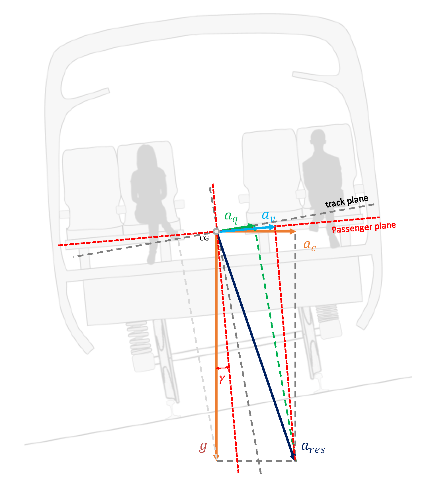
In a curve and due to the centrifugal force , lateral acceleration acts transversely to the direction of the railway track. The cant partially reduces the total lateral acceleration, but if the train speed is not V e q , there still is an uncompensated lateral acceleration ( a q ) that has to be assumed by the passenger, generating the consequent loss in comfort. Assuming that the total acceleration a c = V 2 R is the one compensated by the cant a c p = g D e plus the uncompensated ( a q ) , then:
a c = a c p + a q a q = V 2 R g D e
This uncompensated acceleration is closely related to passenger comfort. However, the uncompensated acceleration that acts on passengers is usually different than a q . This is because we have supposed that the passenger plane in the train (x-axis) is parallel to the track plane, but we have not taken into consideration the suspension. The shock absorbers may change the axis inclination, causing an effect of reduction in the cant for passengers, consequently reducing their comfort (see Figure 3).
To represent this effect, Equation (5) represents the uncompensated acceleration acting on the passenger’s plane due to cant deficiency and cant excess:
a v = a q 1 + s
where s is the souplesse coefficient; i.e., the coefficient of roll flexibility that depends on the vehicle characteristics (type of train). For example, HSR trains usually have a value of s = 0.2 , and some older conventional trains can reach values of s = 0.4 . For example, Talgo trains are designed to compensate for this effect and can even increase the passenger’s comfort, reaching values of s = 0.3 (see, for example, Guillén et al. [14,15]).
Note that therefore a v a q when s is negative (tilted trains), and a v a q when s is positive.

2.1.2. Parameters Involved in Defining the Transition Curve (Clothoid)

A transition curve is a mathematically calculated curve in the plan design of railway tracks, placed between straight sections to smooth the undesirable effects of the appearance and disappearance of centrifugal force and to improve the transition into the cant. Note, that the common method of building the transition is by raising the outer rail because is a better way to maintain the ballast width.
Among all the alternatives, the most used curve is the clothoid (see Brustad and Dalmo [16]), the general expression of which is A 2 = R L , which, in order to decide the length L chosen by the designers for the alignment, must meet some geometrical and functional conditions (see Section 2.2).

2.2. Design Constraints for Railway Track Curves

This section deals with a deep analysis of constraints that are used to define the limits of the parameters involved in designing horizontal alignment (i.e., radius of curves, clothoids, and cants) for mixed-speed train traffic. The three main constraints involved are: (1) maintaining a minimum passenger comfort, (2) guaranteeing the safety of every train that will use the curve, and (3) minimizing the maintenance costs during all the infrastructure lifetimes.

2.2.1. The Passenger Comfort

Rail passengers expect to safely and comfortably stand up and walk around the car during their journey. Some authors; for example, Lauriks G et al. [17], have studied this; among other factors for passenger trains, the primary comfort issue is the uncompensated lateral acceleration, which is directly related to the design parameters of the curve. From Equations (4) and (5), we can obtain:
V a v m a x 1 + s + g D e R ,
which is the maximum allowable speed in a curve as a function of the horizontal alignment design ( R and D ), of the desired level of comfort for the passengers ( a v m a x ), the quality of the train ( s ), and the track characteristics ( e ). This is a very important expression when designing the radii and the cant of a curve, depending on the desired allowed speed while attending to passengers’ comfort issues.
Example 2.
Let us analyze a train (let us use the Talgo T350 cars used in Spain. See for example Renfe [18]) ( V = 350   k m / h ; s = 0.3 ) using a mixed-speed traffic railway line. Let us assume that a curve section with the usually used design parameters in Spain; i.e., D = 140   m m and e = 1500   m m , and let us set a v m a x = 1   m / s 2 ; thus, using Equation (6) to obtain the minimum radius, we obtain R 4030   m . However, with these parameters and when using (2),  I = 229   m m , which is a value that could be high for I because it may lead to track lateral stability problems (see Section 2.2.2), so the radius must be increased. In particular, in Spain, R = 7250   m is the most commonly used. In addition, this example points out that the influence of the souplesse is neglected when one wants to obtain higher allowed speeds when designing high-speed railway lines, because the obtained cant deficiency is very high no matter the value of s for low radii (where the tilted trains have many advantages). This will be clearer when using our proposed method in Section 3.

2.2.2. The Lateral Stability

Railways are linear structures that are subject to static, quasistatic, and dynamic forces from trains and different weather conditions. A train that moves in a curve exerts a lateral load due to:
  • Quasistatic forces mainly derived from unbalanced cant and thermal loads,
  • Dynamic reasons mainly derived from the track quality, and
  • The crosswind that may appear.
Then, if it is assumed that those forces act entirely on one of the rails (depending on whether the train enters with cant excess or cant deficiency), the following equation can be derived (see, for example, Esveld [12] or López Pita [13]):
H c = 1.2 2 Q I e + 2 Q V 1200 + H w ,
where again, some parameters involved in the radius and cant design appear in this formula. Regarding the wind load ( H w ), although each train has its own characteristic wind curve (CWC), and some standards exist to limit the train speed depending on the wind (Yu et al. [19]), the Beaufort scale (Wallbrink and Koek [20]) proposes a relationship between the speed of the wind and the pressure against a surface (in our case, it should be the surface of the side view of a train’s coach), which can be used to obtain H w .
To ensure the safe circulation in a curve, the transverse resistance L m i n of the track must be obtained. For example, Prud’homme developed the following equation (see, for example, Hasan [21]):
L m i n = β 1 + 2 Q 3 ,
where L m i n is the minimum resistance that the track will have, 2 Q is the heaviest train axle load, and β is the coefficient to take care of track maintenance and layout of tracks which is 1.5 for a concrete sleeper. To ensure a sufficient level of stability,   L m i n H c > δ   , defined as the safety factor of lateral track stability, which is desirable to be δ > 1.5 . Therefore, to ensure the lateral stability of the tracks for high-speed trains, the cant deficiency must be limited.
Example 3.
Let us analyze a train as in Example 1 (the Talgo T350 (Renfe) [18] has a lateral surface of 13.14 × 3.365 = 47.96 m2) ( V = 350   k m / h ) using a mixed-speed traffic railway line while a high wind of 60 km/h is blowing (#7 on the Beaufort scale, corresponding to a pressure of 33 daN/m2). Assume that the curve section has the usual design parameters in Spain ( R = 7250   m ;   D = 140   m m ; and hence using (5), I = 60   m m ) and the freight trains have  2 Q = 20   T n to obtain  L m i n from Equation (8). Those data lead us to δ = 1.65 , justifying this design as valid for the lateral stability constraint. In fact, the limitation according to the Spanish standards (Adif [6]) is that I m a x = 80 mm, therefore this design fulfilled the standards for this train.

2.2.3. Maintenance Cost

It is well known that the cyclic loads that both heavy and high-speed trains transmit to the platform deteriorate the track geometry, producing high maintenance costs (see Gallego et al. [22] for a good review of deterioration models). Although maintenance costs depend on many factors, most models establish a relationship between the settlement and the number of load cycles (Grossoni et al. [23]). Hence, in general, and following the notation in Figure 1, one can assume that the total loads in each rail ( C i and   C e ) can be divided into three terms:
  • Static load Q s , which is simply the static weight of the train in this case, and for convenience, measured by wheel Q .
  • Quasistatic loads Q q , which are the loads appearing while the train travels around a bend such that V V e q (see Table 2).
  • Dynamic overloads Δ Q d , which are closely related to the train speed due to its influence on the effects of the weight of the suspension and nonsuspension masses of the train, the stiffness of the platform, and the maintenance quality of the tracks (see, for example, Gallego et al. [24,25]).
Both static loads and dynamic overloads should be (almost) the same in both rails. However, the quasistatic loads in a curve will not be. According to the equilibrium of forces that appears on the vehicle as shown in Figure 1, this difference in the reactions in each rail will depend on the characteristics of the train (speed, weight, etc.) but also the alignment design (cant and radius).
Table 2 shows the expressions to be used to estimate C i , a and C e , a ; i.e., the loads that each axle ( a ) exerts on each rail ( i inner and e outer) as a function of I and E ; i.e., as a function of the alignment design and the characteristics of each train. Table 2 also highlights the importance of considering the traffic distribution (mixed-speed and mixed-load trains) that are going to use the track when designing the curve. Note that if the number of axles of slow trains is much higher than those of fast trains and the radius and cant are not well chosen, the cumulative loads in a certain time ( t ) will be very different in each rail due to the sign of the quasistatic loads.
Table 2. Expression to quantify each load cycle (a) on each rail as a function of I and E.
Inner Rail Load (Ci,a)Outer Rail Load (Ce,a)
If cant deficiency (I) Q 2 Q · I · h c e 2 + Δ Q d Q + 2 Q · I · h c e 2 + Δ Q d
If cant excess (E) Q + 2 Q · E · h c e 2 + Δ Q d Q 2 Q · E · h c e 2 + Δ Q d
Therefore, to reduce the maintenance costs during the operation life due to a different settlement in each rail of the curve, the design radii and cant must be chosen so that the cumulative loads in a certain period of time ( t ) are similar in both rails; that is:
a C i , a t a C e , a t = γ ,
where γ should be as close as possible to 1.
Example 4.
Let us use the same curve as in Examples 1 and 2 ( R = 7250   m ;   D = 140   m m ), where in this case, the line is intended for mixed-traffic train operation (passengers and freight). The train for the passenger is again the Talgo T350; i.e., 16 axles, 2 Q = 16 Tn/axle and h c   = 1.2 m, 20 circulation/way, V = 350 km/h. The freight trains that use the line have two locomotives and 36 wagons; i.e., 152 axles, 2 Q   = 20 Tn/axle and h c   = 1.5 m, 10 circulation/way V = 80 km/h. With this, using Equation (2) for passenger trains, I = 60   m m ; and using Equation (3) for freight trains, E = 130   m m . With this, using as reference the formulas in Table 2 (for the sake of simplicity, we used the Prud’homme formulas to obtain Δ Q d (for more details on this expression, see, for example, Balmaseda et al. [26])), γ = 1.34, meaning that due to this high value, each day the inner rail was 34% overloaded, which may cause serious problems in maintenance. For that reason, standards usually limit the cant excess value to 80–90 mm. However, to fulfill this limitation, the freight trains must run at 190–175 km/h, which makes no sense for this type of train. However, even with this, due to the high number of wagons compared with the number of passenger cars, γ = 1.20, which is still a high value. Therefore, the design criteria with this limit must be also revised.

2.3. Design Constraints for Railway Track Clothoid

As it is well known, the clothoid is the most widely used transition curve between straight and circular alignments, not only for railway design but also for roadways (see, for example, Meek and Walton [27]). In the case of this paper, the constraints for railway track design are as follows:
  • Geometrical limitations:
    It must be tangent to the straight for one side and to the circular curve on the other.
    It must have the same curvature as the straight (0) and the curve (1/R).
    It must have a continuous change in curvature.
    The length of the clothoid must be defined to minimize the cant wrap at the end of the transition, and for this, a limit for the cant gradient ( c 1 [mm/m]) must be set. For this:
    Δ D Δ L c 1 L D c 1
  • Functional conditions:
    To avoid both dynamic problems with the rolling stock and comfort problems with passengers, the ascendent speed ( c 2 [mm/s]) of the train’s outer wheel during the transition must be limited. Therefore:
    Δ D Δ t c 2 L D c 2 V
    To ensure a smooth variation in uncompensated acceleration, the variation in this parameter with time is limited. In other words, the rate of cant deficiency variation ( c 3 [mm/s]) is limited. Therefore:
    Δ I Δ t c 3 L V 2 · e R · g D V c 3
The values of c 1 , c 2 , and c 3 are defined in the corresponding standards according to the maintenance experience and comfort tests.
An interesting question appears when deciding which values for V and D should be used to design the clothoid length. It is straightforward to see that to ensure that all the trains that use the clothoid can meet the standards, the used speed in the previous formulas should be the maximum allowed in the line. On the other side, one can be tempted to use the design value for D , and this is a mistake. Note that when tamping the ballasted track, the cant can be easily modified during the lifetime of the line. Therefore, the used cant to obtain the length should be carefully chosen to ensure that the clothoid meets the standards no matter the real cant.
To clarify these issues, the example below develops a case study using the Spanish standard (Adif [6]).
Example 5.
Continuing with the previous examples; i.e., V = 350   k m / h , R = 7250   m , and D = 140   m m , but in this case, let us assume that due to an increase in the number of freight trains, in any moment of the operation life, the railway administration decides to redefine the cant and set D = 100   m m . Table 3 shows the results after applying the formulas developed in this section.
Table 3. Examples of obtaining the clothoid length according to the Spanish standard.
ParameterParameter ValueClothoid Length for
D = 140 mm
Clothoid Length for
D = 100 mm
c 1 1 mm/m140 m100 m
c 2 50 mm/s272 m195 m
c 3 30 mm/s193 m323 m
Note that at the beginning (with D = 140   mm ), the length should be set as L = 272   m due to the ascent speed during the cant transition. If, after a certain period of operation, the cant is changed to 100 mm, now, due to the rate of cant deficiency variation, the length should be 323 m. Therefore, for such a case, since the clothoid was already constructed, it will not meet standards, and high-speed trains should run at a slower speed (in this case, from Equation (12), V 335   km / h ).
To sum up, designing a clothoid is not a straightforward issue, and it deserves better care during the design phase. This paper proposes a method to deal with this issue.

2.4. Review of the Design Parameters Limitation of Several Technical Standards

This section is aimed at analyzing the standards of various countries and a few organizations, including those of:
  • Spain, according to Spanish standards (Adif [6]).
  • The USA, Germany, France, Japan, and Sweden, according to (Rakoczy et al.) [3].
  • Technical Specification for Interoperability (TSI) (European Association for Railway Interoperability (AEIF) [28]).
  • Committee for European Standardization (CEN) (European Committee for Standardization (CEN) [29]).
  • Rail Baltic (railway infrastructure project to link Estonia, Latvia, and Lithuania with Poland) (Ernst and Young [30]).
  • (Russia, Slovakia, Ukraine) from Contact Group of the Organization for Cooperation between Railways (OSJD) with the European Union Agency for Railways (ERA) (OSJD and (ERA)), [31].
Table 4 summarizes the limits that these standards establish for the horizontal alignment design of a railway track depending on the expected traffic type; i.e., high-speed railway (HSR), medium-speed railway (MSR), mixed passenger–freight traffic (P+F), and solely designed for freight traffic (F). The table shows the design speed (column 4), as well as several technical standards limitations in railway design, as noted above (columns 5–10).
The design of mixed-speed traffic railway lines is a very complex task from the aspect of horizontal alignment determination that should go further than just meeting some standards. The proof of this is, as Table 4 shows, that there is not a clear method nor limits for parameters to design such types of lines. What should be clear is that the selected parameters must ensure ride comfort for passengers and safety for all vehicle types, and all these should be within a minimum investment in maintenance.
To meet these requirements, the next section proposes a new methodology to design mixed-speed railway lines and attempts to point out all the requirements in an easy way.

3. The Proposed Methodology

There is a great number of variables and constraints involved in the design of a railway track, and it is never easy when considering all of them. In an attempt to ease this task, in this section we propose a novel methodology based on a graphical analysis of the constraints involved in the design. Since this type of civil engineering problem does not have unique solution, we believe that the way to choose the best one is to propose a group of valid alternatives for the railway line design and then compare them to choose the one that fits better with the project requirements. Therefore, the formal complete methodology is as follows:
  • Propose a number of alignment alternatives to be developed with a proper design software (in the case of this paper, we used Istram-Ispol). For each one:
    • The first step should be to decide which cant law have to be used; i.e., a relationship that provides a cant as a function of the radius of the curve. This decision and the project speed will condition the value of the design parameters including the radii and also the clothoids.
    • In the second step, a novel graphical representation to decide which radii should better fit with the requirements of the design is presented. With it, we intend to have a single picture of all the parameters, equations, and constraints involved in the design, which will allow us to make better decisions.
    • Once the radius and the cant of the curve are decided, the third step is intended to design the clothoid. For this, another graphical method is proposed in order to design a flexible clothoid while taking into account not only the current traffic conditions, but also that it should fit with future possible scenarios.
  • Compare the alternatives using some quantitative figures to finally decide which one is the best. These figures can be those noted in Section 2.
In view of the above, this section is aimed to describe the novel aspects of the methodology (items a, b, and c), leaving the full application of the methodology for the case study in Section 4.

3.1. Defining the Criteria to Design the Cant

Deciding which cant is going to be used in a curve is not an easy task. In fact, proof of this is that many standards propose different criteria to define the cant while trying to consider somehow the operation conditions of the line. Next, some of these criteria are explained to analyze the effects in the final design.

3.1.1. The 2/3 of the Equilibrium Cant Method

For many years (and even in the currently proposed methodology in Adif [6]), the Spanish standards have recommended using the following expression for the design cant:
D = 2 3 · D e q · V m a x = 2 3 · V m a x 2 R · e g
This criterion establishes the design cant as 2/3 of the equilibrium cant for the maximum allowed speed, with the aim (according to the standard) of taking into account the slowest trains. The problem with this criterion is that it does not take into consideration the traffic distribution that is going to use the railway line or the speed distribution. This criterion might have been fine in the mid-20th century, when the speed of the fastest train was 140 km/h and the slowest was at 80 km/h. However, when the gap between speeds is 100–350 km/h, this criterion should be revised, since for fast trains, the resulting cant may lead to a low cant deficiency, whereas slow trains may have a large cant excess.

3.1.2. The Root-Mean-Squared Speed Method

To solve some of the problems derived from the operational speed distribution, other standards recommend using the equilibrium cant for the root-mean-squared speed of the fastest and the slowest train that is going to operate the line as the design cant. That is:
D = D e q V m = V m 2 R · e g   |   V m = V m a x 2 + V m i n 2 2
This criterion takes into consideration the gap between the highest and lowest speeds, but neither speed takes into consideration the traffic distribution. If this criterion is applied, the design cant is the same for the case of one service of a high-speed train and 20 freight trains as if the operation is of 20 services of high-speed trains and only one freight train. Depending on the case, this may cause maintenance problems, as Section 2.2.3 shows.

3.1.3. The Alpha Method

The Union Internationale des Chemins de Fer (UIC), an international association aimed at cooperation between the main railway administrations in the world, proposed an easy-to-use formula as follows:
D mm = α · V m a x 2 km / h R m
This criterion takes into consideration the traffic distribution with a new parameter α that depends on the traffic distribution: α 6.5 ; 8 for a mixed-speed-traffic railway line and α 8 ; 10 for the case in which the gap between fast trains and slow trains is low. This equation allows the designer to analyse several cant distributions and their implications in the design parameter by just adjusting α .
Note that Equation (15) is a generalization of Equation (13), because (13) implicitly applies a value of α = 7.9 , which is a proof that it should not be applied to design the cant of mixed-speed railway lines.

3.1.4. The Modified Root-Mean-Squared Method

This criterion takes into consideration traffic distribution with different speeds, and this method proposed to use the equilibrium cant for a weighted root-mean-square speed V * . A good weight factor ( p i ) can be the number of axles of each type of train i that will use the track at a speed ( V i ) ; that is:
D = D e q V * = V * 2 R e g | V * = i n p i V i 2 i n p i
This design cant is aimed at implicitly obtaining a value of γ 1 in (9); i.e., it attempts to minimize uneven wear on both rails. The drawback is that if the number of slow train axles is much larger than of fast trains, the obtained cant will be low, and hence the passenger comfort will decrease and the cant deficiency will increase.

3.2. Graphical Representation to Define the Cant and the Radii

Let us explain the method using a particular example in terms of traffic and a criterion for designing the cant. The train characteristics and the expected daily traffic are shown in Table 5.
Our proposal is presented In Figure 4, where the x-axis is the radius in meters, the left y-axis is the speed in kilometers per hour, and the right y-axis is the cant, cant excess, and cant deficiency in meters.
The lines in the figure are as follows:
  • The black line represents the proposed design cant as a function of the radii and according to one of the criteria defined in Section 3.1. In this particular case, 2/3 of the equilibrium cant method is represented. Note that since D m a x = 140   mm , the line has 2 parts:
D = D m a x i f R < 2 3 V m a x 2 · e D m a x · g D = 2 3 V m a x 2 · e R · g i f R 2 3 V m a x 2 · e D m a x · g
For this particular case, the design cant should be D m a x = 140   mm up to R 6940   m , and then the cant progressively decreases, but always with relatively high values. Note that this criterion is devoted to obtaining lower cant deficiencies for fast trains, and even for radii near 10,000   m , the cant is above 100   mm .
  • The orange lines represent the design curves for the high-speed trains used as the design cant for the curve in (17). Particularly:
    The solid orange line represents the maximum allowed speed for this train ( V 1 ) as a function of the radii according to Equation (6) and assuming a v m a x = 1   m / s 2 . Again, and due to the maximum speed for this type of train, this line has two parts:
    V 1 a v m a x 1 + s 1 + g D e R i f R < V 1 m a x 2 a v m a x 1 + s 1 + g D e V 1 V 1 m a x i f R V 1 m a x 2 a v m a x 1 + s 1 + g D e
    The resultant cant deficiency is a dashed orange line according to Equation (2). In this case, the curve has three parts:
    I 1 = a v m a x e 1 + s 1 g i f R < V 1 m a x 2 a v m a x 1 + s 1 + g D m a x e I 1 = V 1 m a x 2 R e g D m a x i f V 1 m a x 2 a v m a x 1 + s 1 + g D m a x e R < 2 3 V m a x 2 · e D m a x · g I 1 = V 1 m a x 2 R e g D i f R 2 3 V m a x 2 · e D m a x · g
The first section is a constant straight line because the cant curve is constant, and the maximum speed is the maximum allowed. For this case, I = 191   mm up to R 4400   m . The second section is a very steep slope curve because while the radii increased, both the speed and the cant were constants and the maximum. Finally, the last part has a low slope curve because the cant law criteria for this section was a decreasing curve. Using these equations and Figure 4, we can observe that the sensitivity of the cant deficiency concerning the radii was higher in the second part than in the others. This is very important, because if a designer is looking for a lower value for the cant deficiency by increasing the design radius, better results will be obtained in this range of radii. For example, increasing the design radius from 5500 to 6000 m produces a reduction in I from 125 mm to 100 mm. However, if the same increase is applied (500 m) from 8000 to 8500 m, the reduction in I is just from 65 to 60 mm, and it may be worth changing the design cant criterion.
  • The purple lines represent the design curves for the shuttle train also using Equation (13) as the cant criteria. Specifically:
    The maximum allowed speed as a function of the radii is represented as a solid line that also has two parts with the same expressions as in Equation (18), but using V 2 m a x instead V 1 m a x . Note that in this case, because s = 0.2 instead of s = 0.3 , the maximum allowed speed has to be lower to meet the limit of a v m a x = 1 m s 2 . In any case, when designing high-speed railway lines, this limit is never reached, no matter the type of train, due to the high cant deficiency obtained for those combinations of R ,   V , and D , having then to increase the radius to decrease I .
    The resultant cant deficiency is a dashed line according to Equation (2). Note that for this type of train with V 2 m a x = 250   km / h , and since V 2 m a x < 2 3 V m a x , the shape of the curve has some interesting features, and four sections can be defined as follows:
    I 2 = a v m a x e 1 + s 2 g i f R < V m a x 2 a v m a x 1 + s 2 + g D m a x e I 2 = V 2 m a x 2 R e g D m a x i f V m a x 2 a v m a x 1 + s 2 + g D m a x e R < V 2 m a x 2 · e D m a x · g E 2 = D m a x V 2 m a x 2 R e g i f V 2 m a x 2 · e D m a x · g R < 2 3 V m a x 2 · e D m a x · g E 2 = D V 2 m a x 2 R e g       i f                                                 R 2 3 V m a x 2 · e D m a x · g
The first and second sections have a shape and features like those exposed to the first type of train. It is interesting to analyze that using the radius, which makes I 2 = 0 ; the third section indicates that this train would enter with cant excess (Equation (3)), which increases while the cant is constant and maximum. After that, in the fourth section, the cant excess decreases with a slope that depends on the cant criteria and the train speed. This is very interesting from a conservation point of view because, with this criterion and R > 5275   m , the shuttle trains circulate with cant excess improving or worsening the maintenance coefficient γ (see Equation (9)) depending on the traffic.
  • The green lines represent the design curves for the freight trains. For the sake of simplicity, we have avoided the analysis of small radii, where cant deficiency may appear for slow trains:
    From Equation (9) and assuming a certain limit for the cant excess ( E p m a x ), the minimum allowed speed is represented as a light solid line according to the expressions below:
    V 3 D m a x E m a x g R e i f 0 < R < 2 3 V m a x 2 · e D m a x · g V 3 D E m a x g R e i f 2 3 V m a x 2 · e D m a x · g R < 2 3 V m a x 2 · e E m a x · g V 3 0 i f R 2 3 V m a x 2 · e E m a x · g
Note that assuming V 3 m a x as the maximum speed for freight trains from Equation (21) and E p m a x as the maximum allowed by the standard, one can conclude that the interval of radii that those trains can circulate is as follows:
R ( V 3 m a x ) 2 e D m a x E m a x g ; 2 3 V m a x 2 ( V 3 m a x ) 2 e g E m a x ,
That, for the case represented in Figure 4, implies that for E m a x = 80   mm , we need to design with R 10,700   m and D 90   mm , which is far from the commonly used R 7250   m .
The resultant cant excess is a long dashed line, according to Equation (3).
The proposed graphical representation shown in Figure 4 includes in just one picture all the analytical information presented in this section, allowing a technician to see the big picture of the problem they are facing, and hence is a powerful tool to find the best solution possible. For example, with all the data exposed above, the minimum radius for which both passenger trains can enter at their maximum speed is R 4000   m , but this solution has a large value of uncompensated acceleration for both. If we want to meet the Spanish standard (see Table 4), we must obtain a design such that I m a x = 80   mm . Therefore, fixing this value for the Talgo T350 on the left axis and searching for the orange cant deficiency line, we obtain R 6620   m .
However, we also assumed that five freight trains with a maximum speed V 3 m a x = 100   km / h   will also use the lane. Therefore, R 10,700   m is the lower radii at which all trains circulate at their maximum speed obtained in Figure 4; that is, D = 90   mm , I 1 = 45   mm , E 2 = 21   mm , and E 3 = 80   mm .
The next step should befit this radius in the terrain with the rest of the alignments in the corridor, and such a radius may be very high for this purpose. Therefore, this may lead us to reconsider the design in different ways, such as:
  • By supposing that the slowest train travels at, for example, 180 km/h, which is the maximum of the minimum speed curve (the green light curve). However, it may be difficult for rail freight transport to be profitable at those speeds.
  • By changing the limit value of the cant excess imposed by the standard, the invalid radii would be reduced. This may have other consequences; for example, Equation (9). The last solution is to modify all the designs and change the cant definition criteria.
Therefore, using our proposed method, we could easily evaluate several cant definition methods and compare the values of the design parameters of the alignment and choose the best solution depending on the project objectives.
For example, Figure 5 shows the results after applying four different criteria to design the cant and using R = 9000   m to compare the results. In addition, Table 6 shows the quantitative results used to compare which method provided better results depending on the objectives of the project. For example, in terms of maintenance objectives, the modified root-mean-squared method provided much better results than the other three laws, resulting in γ = 1.03 . Note that the weighted mean square speed that resulted was 170 km/h, so the cants for that criterion obviously were much lower than those obtained for others, compensating then for the damage that this high amount of freight axles may cause to the track. In addition, the minimum speed was below 100 km/h; therefore, the freight train could circulate through all the radii without violating the limit of cant excess. However, this law implied that the passengers of the high-speed train may travel a little bit more uncomfortably compared with other laws with a higher cant ( a v = 0.56   m / s 2 vs. a v = 0.23   m / s 2 ). Finally, although in all cases the delta coefficient was higher than 1.5 (as in previous sections, we considered a wind speed of 60 km/h to obtain δ), it was true that for the modified root-mean-squared Method and the Talgo T350, this coefficient may have appeared low, but for days with a lower wind speed, the value would increase.
From this point on, the decision is on the railway administration side. The purpose of these examples was to show the complexity of the design of the railway layout, especially for tracks for mixed traffic of high-speed trains with freight trains, and to assist in deciding whether to use one method or another to define the radii and cants while studying the implications that this will have both in operation and maintenance.
Table 6. Data to compare the performance of each designs by using different cant criteria.
Criterium to Define the Cant
Parameter to Analyze2/3 of the Equilibrium CantAlpha Method
( α   =   6.5 )
Root-Mean-Squared Speed MethodModified Root-Mean-Squared Method
CantD (mm)110908540
Coefficient maintenance cost γ 1.171.131.121.03
High-speed train (V1 = 350 km/h)
Cant deficiency I 1   (mm)517275123
Uncompensated acceleration a q (m/s2)0.330.460.490.80
Uncompensated acceleration in the passenger a v (m/s2)0.230.320.350.56
Coefficient lateral stability δ 1.801.731.711.57
Shuttle train (V2 = 250 km/h)
Cant deficiency I 2   (mm)---44
Cant excess E 2   (mm)2563-
Uncompensated acceleration a q (m/s2)0.180.050.020.29
Uncompensated acceleration in the passenger a v (m/s2)0.220.060.020.35
Coefficient lateral stability δ 2.392.532.562.59
Freight train (V3 = 100 km/h)
Cant excess E 3   (mm)97757225
Uncompensated acceleration a q (m/s2)0.630.500.470.16
Coefficient lateral stability δ 3.023.573.374.33

3.3. Graphical Representation to Define the Length of the Clothoid

As noted in Section 2.3, when calculating the length of a clothoid, one has to meet the three criteria stated by Equations (10)–(12).
On the other hand, to decide the length of the clothoid, the future traffic conditions must be considered because if they change at any moment in the infrastructure’s lifetime, the cant can be easily changed to improve both the operational and maintenance conditions.
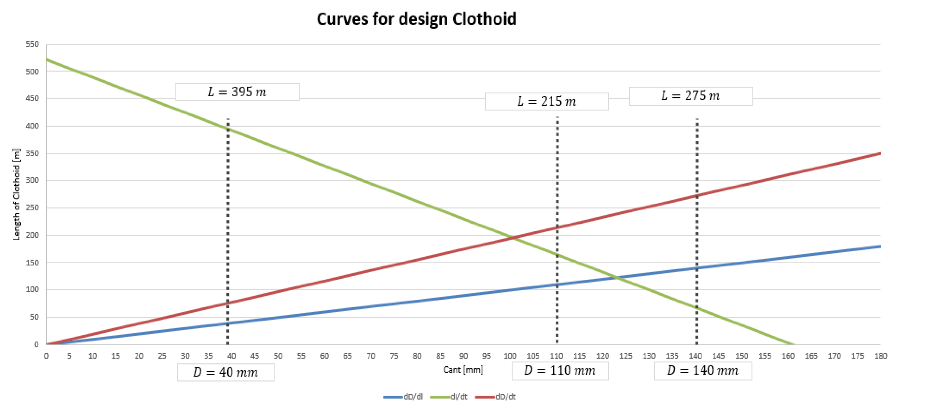
To ease the difficulty in decision making when designing a flexible clothoid, we propose Figure 6, which shows, for a given R = 9000   m , the length of the clothoid as a function of the cant and for each of the constraints (lines in blue, green, and red). Let us assume that we have decided to use D = 110   mm ; therefore, the most restrictive condition for this cant is the ascended speed (red line), resulting in a minimum length of L m i n = 215   m .
However, in the analysis developed in the previous section depending on the criteria, the range for cants was D = 40 ; 110   mm   (see Table 6). Therefore, if in the future we decide to change the cant to D = 40   mm , a length L m i n = 395   m should be used (in this case due to the rate of cant deficiency (green line)) but this would not be possible because the clothoid would be short ( 215   m ) and would not meet the standards.
To sum up, in this example we recommend designing the clothoid with L = 395   m , which, in addition, is even valid for the case in which, for any reason, the line was destined only for passenger trains at V = 350   km / h , and the cant would have to be changed to D = 140   mm .

4. Case Study

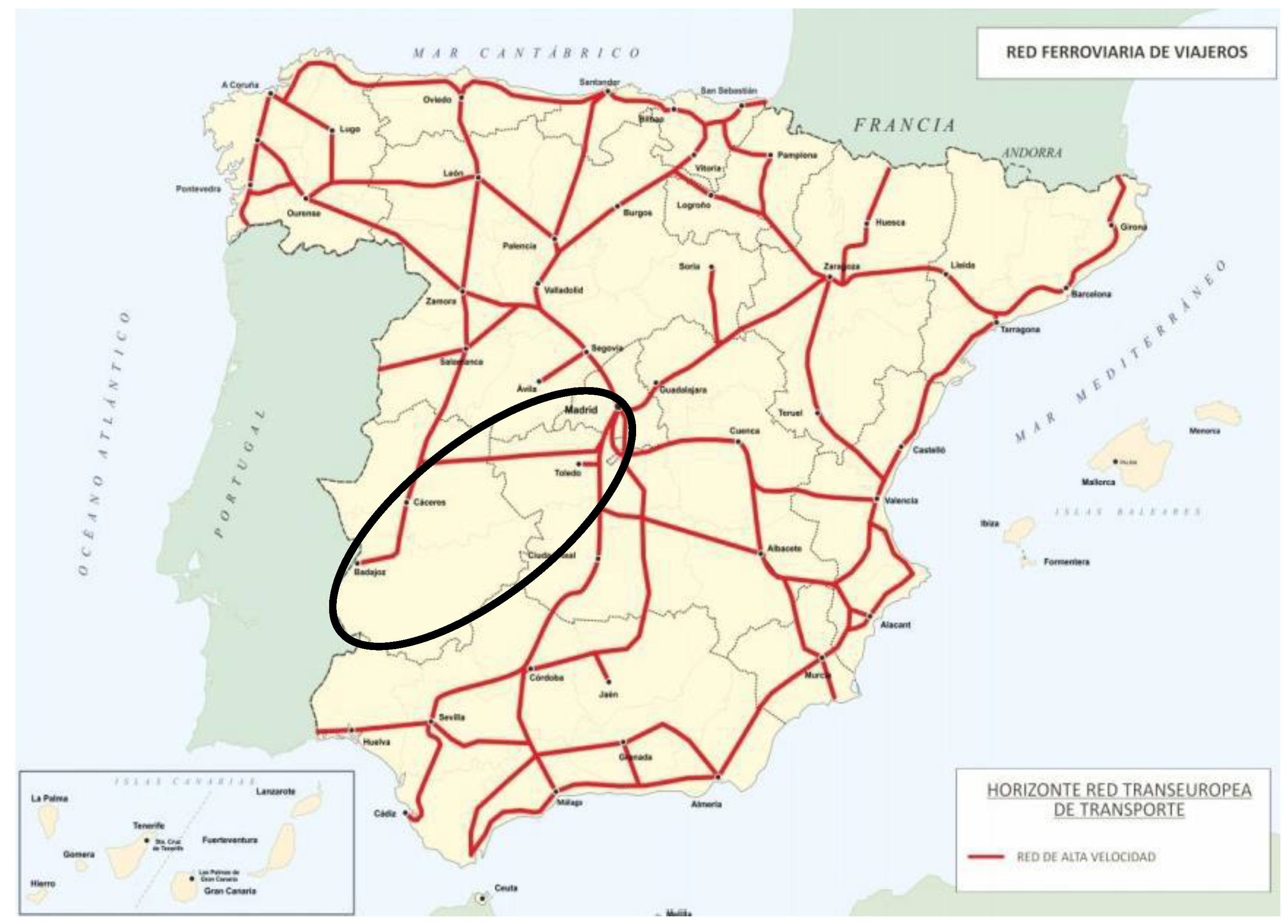
As a case study, we chose an ongoing project that is being developed in Spain between Madrid and the Portugal border. The objective of the project is the construction of a new high-speed line between Madrid and Oropesa that is included in the planned Trans-European Transport Network for railways and is planned to be used by mixed-speed traffic, and particularly high-speed trains for passengers and freight transportation (see Figure 7).
This section aims to analyze one of the proposed layout alternatives for this corridor and compare it with some others designed using the proposed method in this paper. In addition, all the alternatives were implemented in the field using the software Istram-Ispol [34].

4.1. Location and Description of the Considered Section

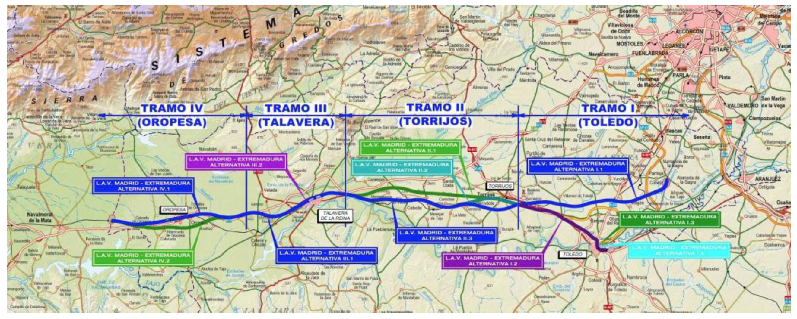
The line begin with the connection with the high-speed line Madrid–Sevilla and finishes in Oropesa. In Adif [33], an analysis and comparison of alternatives for this line were developed by dividing the line into four sections and proposing two and four alignments (see Figure 8). In this paper, we studied the alignment composed of the following sections:
  • Alternative I.1. Corresponding with the blue line of Section I. This section connects with the high-speed line Madrid–Sevilla and finishes in Torrijos.
  • Alternative II.3. Corresponding with the blue line of Section II, we studied just the first half of this section. It connects with Alternative I.1 in Torrijos and finishes in Talavera de la Reina.
The corridor will have characteristics to allow high-speed traffic between areas with potential high traffic, correcting present situations of a lack of accessibility. This line responds to the need to achieve a direct high-speed connection between Extremadura–Madrid and provide direct access at high speed to Portugal, thus structuring high-speed rail communications in the west of Spain. The corridor has a main stop in Talavera de la Reina that is going to be served with regional shuttle services (Avant) to and from Madrid.
In this frame, Adif [33] forecasted future traffic for 2030 and 2050 (see Table 7), which was the basic starting point for our model to estimate the traffic in the corridor.
The assumptions were as follows:
  • The trains that will operate the corridor will be the Renfe’s S-102 series (Talgo T350) for high-speed services (AVE), and the S-114 series for shuttle services (Avant). In addition, we included freight trains. The characteristics of those trains are given in Table 5.
  • The capacity of the trains was 320 passengers for S-102 and 230 for S-114.
  • The mean occupancy grade for both AVE and Avant trains was 60%.
  • The effective schedule for traveler trains will be from 6:00 a.m. to 10:00 p.m. (16 effective hours); therefore, between 10:00 p.m. and 6:00 a.m., freight trains could use the line while respecting at least 3 h daily for maintenance. With this, the estimated traffic is shown in Table 7. Regarding freights trains, we understand that the Lisbon–Madrid corridor is an important one because it could join some Portuguese ports with Madrid and the rest of Europe. So, freight transport by train could be very competitive, and therefore we estimated 8 freight trains each way per day in this line for 2030 and 10 for 2050.

4.2. Proposing Some Alternatives to Be Compared with the Original Project

In this section, we will show several alternatives that were compared with the original project to enhance the applicability of our proposed method.

4.2.1. Alternative 0: The Proposed Alternative in the Original Project

The alternatives proposed in Adif [33] were designed (using the limits for the design parameters of the old IGP standard by Adif [35]) while assuming I L i m = 60   mm and D m a x = 140   mm , then imposing V = 350   km / h and using Equation (2) to obtain R = 7250   m , which is the radius commonly used for this high-speed railway line. All curves of the track had a radius of 7250 m, except for one curve that was 7750 m with a clothoid of 460 m and a cant of 130 mm, and another curve of 8500 m with a clothoid of 355 m and a cant of 110 mm. However, even when imposing the limit of the current standard of E L i m = 90   mm , the freight trains must circulate at V = 165   km / h , which may be far from the current commercial speeds for freight trains.
Regarding the length of the clothoid, L = 460   m , which may appear to be long. The reason for this is found in the old standard, in which an ascended speed restriction of c 2 = 30   mm / seg was imposed.

4.2.2. Alternative 1: The Proposed Alignment from the Original Project but a Different Cant Law

In this alternative, we are considered the same design parameters as in the original track, but attempted to meet the cant excess criteria to allow the freight trains to circulate. To do so, we believe that the most flexible criteria to define the cant to face this problem may be the alpha method shown in Figure 9. In this case, when considering α = 6.2 , the cant law was considerably lower and resulted in D = 105   mm to obtain E 3 = 90   mm . The problem here is that the AVE trains would pass the curve with I 1 = 95   mm . The consequences will be analyzed in the next section.
Regarding the clothoid, the project alternative Alternative 0 defined L = 460   m , and since the range of valid cants was D = 60 ; 140 , this provided relatively enough flexibility for the clothoid (see Figure 9).

4.2.3. Alternative 2: Designing Using the 2/3 of the Equilibrium Cant Method

The purpose of this alternative was to use the Spanish traditional method to obtain the minimum radius so that all the trains met the standard and reached their maximum speed. Figure 10 shows that the cant law for this method is high, which implies that the cant deficiency for high-speed trains is low, so the passengers will experience high comfort. However, both shuttles and freight trains will enter with cant excess, and in particular, the maximum allowed cant excess for freight trains and a very large radius. Therefore, for this case, the chosen values were R = 9500   m and D = 105   mm to obtain I 1 = 51   mm , E 2 = 24   mm , and E 3 = 89   mm .
Assuming the previous range of cants D = 60 ; 140 were valid, in this case, the length of the clothoid could be shorter than the previous alternatives, but as Figure 10 shows, it could maintain the flexibility to change the cant. For this particular case, L = 300   m should be chosen.

4.2.4. Alternative 3: Designing Using the Alpha Method

The alpha method proposed by the UIC has been shown to be the most flexible when attempting to find a value objective for a particular parameter. One can iterate the value of α to find the minimum radius that fits with the standard. For example if I L i m = 80   mm and E L i m = 90   mm (see Adif [6]), using α = 6.66 , we find that with R = 7850   m and D = 105   mm , we obtain I 1 = 80   mm , E 2 = 11   mm , and E 3 = 90   mm .
Again, if cants D = 60 ; 140 , the length of the clothoid should be L = 405   m , as Figure 11 shows.

4.2.5. Alternative 4: Designing Using the Modified Root-Mean-Squared Method

By using this method, we aimed to reduce the uncompensated overloads in both rails (see Section 2.2.3) using Equation (16) with the number of axles of each train as weight factors p i . This law provides very low cants (see Figure 12), which produces higher cant deficiencies for the high-speed trains. To maintain this parameter under a certain value of 10 0   mm , we decided to propose R = 10 , 000   m and D = 40   mm , so we obtained I 1 = 105   mm , I 2 = 34   mm , and E 3 = 28   mm . The radius in this case may appear very large, but if the territorial conditions to implement it are not very restrictive, this should not be a problem.
Regarding the clothoid, again the most restrictive constraint was the rate of cant deficiency, which implied that L m i n = 340   m .

4.3. Comparing Alternatives

Table 8 shows the value of all the analyzed parameters, which helped us to compare the alignments of all the alternatives in terms of the constraints for railway track design (see Section 2.2); i.e., comfort, security, and long-term implications regarding the maintenance. Let us point out here that the used value of wind speed (required to obtain values of δ ) was 55 km/h, which was obtained from a statistical analysis of the wind speed in Talavera de la Reina and Toledo from 31 December 2000 to 31 December 2020 (Datosclima) [36]. This value corresponded with a grade 7 on the Beaufort scale, which meant a pressure value of 33 daN/m2.
When comparing the alternatives from the passenger comfort point of view, all alternatives for uncompensated acceleration in the passenger train had values less than ( a v m a x 1   m / s 2 ); therefore, these alternatives satisfied the requirements for the standards for mixed-speed traffic. In the case of mixed-traffic railway lines, the choice of radius must ensure a comfortable ride for passenger vehicles, safe freight transport, and acceptable maintenance costs of railway infrastructure.
Regarding lateral stability, the values of δ for all alternatives and all trains that circulated were δ > 1.5 , so the satisfied desirable value to ensure a sufficient level of stability of the track, even when using the modified root-mean-squared method because we used a very high radius, could maintain this coefficient in a proper range. Finally, when attempting to give an initial opinion on the maintenance cost during the lifetime of each alternative, the proposed γ coefficient was a good tool. The best value was obtained for Alternative 4, being very close to 1, which is a great value for reducing the posterior maintenance costs of vehicle wheels and railway infrastructure. The rest of the alternatives had γ 1.20 , which was a high value. The worst alternative in terms of expected maintenance costs was the current Alternative “0”, which resulted in a value of 1.27, meaning that the traffic might cause a very high overload of the inner rail.
Table 8. Comparison of design parameters and constraints of railway track design curves for each alternative.
Parameter to Analyze# of Alternative
01234
Alpha Method
( α = 6.2 )
2/3 of the Equilibrium CantAlpha Method
( α = 6.66 )
Modified Root-Mean-Squared Method
CantD (mm)14010510510540
Radius R (mm)725072509500785010,000
Clothoid L (mm)460460300405340
Coefficient maintenance cost γ 1.271.191.211.191.07
High - speed   train   ( V 1 = 350 km/h)
Cant deficiency I 1 (mm)60954780105
Uncompensated acceleration a q (m/s2)0.390.420.310.520.68
Uncompensated acceleration in the passenger a v (m/s2)0.270.430.220.360.48
Coefficient lateral stability δ 1.891.761.941.701.73
Shuttle   train   ( V 2 = 250 km/h)
Cant deficiency I 2 (mm)34
Cant excess E 2 (mm)3832711
Uncompensated acceleration a q (m/s2)0.250.020.180.070.22
Uncompensated acceleration in the passenger a v (m/s2)0.300.020.210.090.27
Coefficient lateral stability δ 2.322.562.392.502.35
Freight   train   ( V 3 = 100 km/h)
Cant Excess E 3   (mm)12490939028
Uncompensated acceleration a q (m/s2)0.810.550.600.590.18
Coefficient lateral stability δ 2.713.123.073.114.24
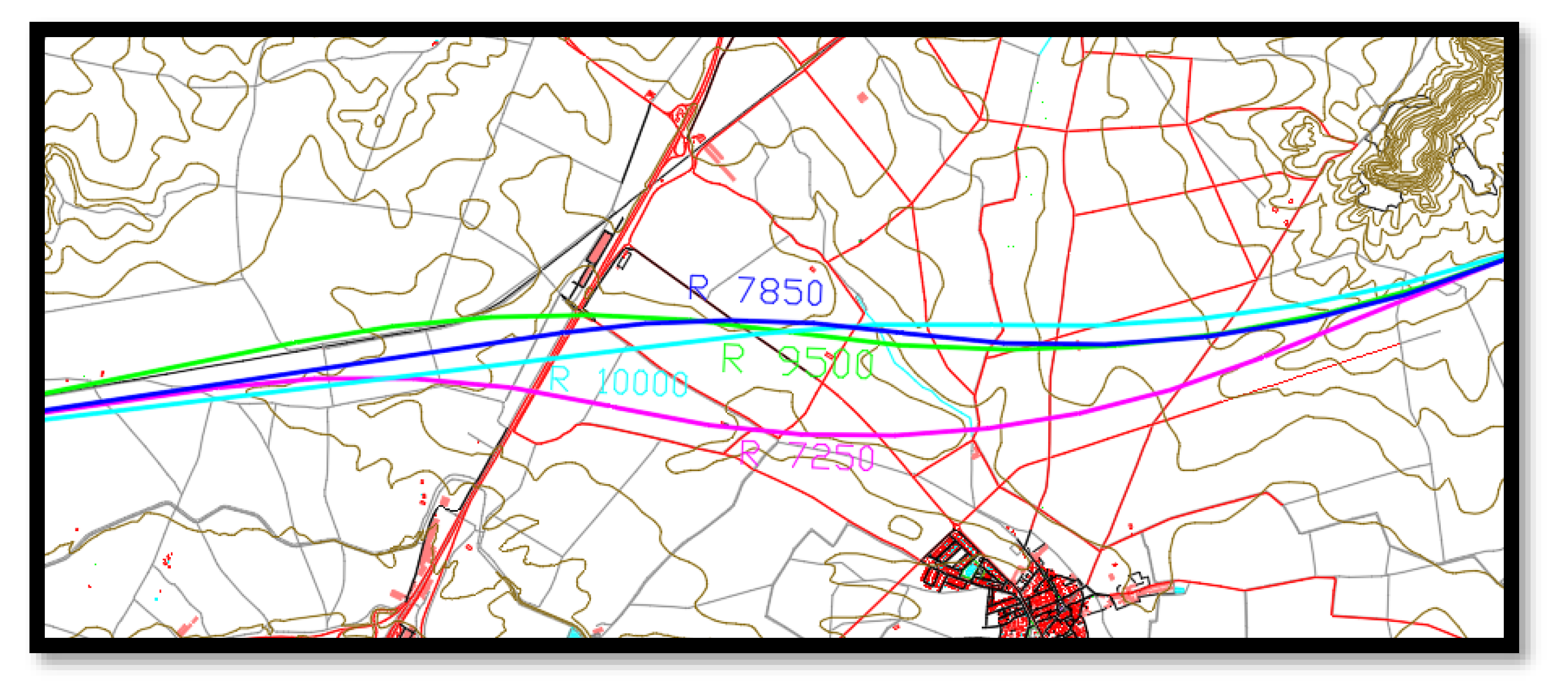
To give a more complete analysis of the alternatives, we used the software Istram-Ispol to analyze if they really could fit with the terrain and the physical constraints of the field. The results are shown in Figure 13, in which all the alternatives are drawn with those proposed in the original project (Adif [33]). We kept the tangents (straight alignments) throughout the corridor, and we only changed the radii and the clothoids of the curves depending on the alternative. The zoomed zone in Figure 14 shows the first curve of the alignment, where we can see that in this particular case, no specific field constraints existed and even the highest radius, R = 10,000   m , could fit with the alignment in almost the same corridor, improving the general performance of the operational period, hence reducing the cost of the infrastructure over its lifetime.
Therefore, we can conclude that the differences between the original track and the alternatives were very low in terms of terrain effect. However, the analysis developed in this section has shown that by choosing the correct design parameters, passenger and freight trains can share high-speed tracks. This method is a tool that aims to help technicians to better invest economic resources to reach the most sustainable solution when designing high-speed railway lines.

5. Conclusions and Future Research

The proposed methodology allowed for a better analysis of the parameters, design criteria, and future implications of several railway alignment alternatives in a very innovative way. This means that we could look for different results or check for better solutions and compare them, whereas other methodologies are very expensive in terms of time. To sum up, the main advantages were:
The graphic method allowed us to see all the design parameters and their limitations in the same figure, and modifications in terms of changing the criteria to design the cant could be very easily analyzed. So, it was very powerful when looking for some alignment alternatives.
We pointed out the importance of explicitly evaluating the passenger comfort, the train lateral stability in curves, and the maintenance cost when designing the curves of the alignment. In particular, nowadays, the maintenance cost for high-speed railway lines can amount to about EUR 3 million per km and year (see, for example, Campos Méndez et al. [37] and Normas Técnicas Vía ADIF [38]). Therefore, taking into account this point in this early phase of the lifetime of the infrastructure is a key point.
The proposed method to define the length of clothoids took into account not only that it must meet the standard for the proposed radius–cant pair, but also the possibility to be valid for an eventual change of the cant that adapts the railway track to a new traffic operation. This is not an evident aspect, because if the length is not well chosen, the speed limit for high-speed trains and/or freight trains might be modified.
Regarding the improvements and future research, we are working on the implementation of the benefits of the BIM methodology to connect the design program Istram with a budget program, as well as with a track deterioration model. With this, we will explicitly take into account the economic implications of the alignment design of a railway track. The time gained with this improvement is enormous, as it is able to create and evaluate several alternatives in a few hours, and accidental mistakes will be reduced because the budget program will directly read the data from the design program.

Author Contributions

Conceptualization, S.S.-C. and I.G.; methodology, all authors; software, S.S.-C., A.A. and J.M.L.-M.; validation, S.S.-C. and I.G.; formal analysis, all authors; investigation, A.A. and J.M.L.-M.; resources, S.S.-C. and I.G.; data curation, A.A. and J.M.L.-M.; writing—original draft preparation, A.A. and S.S.-C.; writing—review and editing, all authors; visualization, A.A. and S.S.-C.; supervision, I.G.; project administration, S.S.-C. and I.G.; funding acquisition, S.S.-C. and I.G. All authors have read and agreed to the published version of the manuscript.

Funding

The Article Processing Charge of this work was paid by the Department of Civil and Building Engineering of the University of Castilla-La Mancha (Spain).

Institutional Review Board Statement

Not applicable.

Informed Consent Statement

Not applicable.

Data Availability Statement

The data presented in this study are available upon request from the corresponding author.

Acknowledgments

We also would like to thank the editor and his team and the anonymous reviewers whose valuable comments contributed to the improvement of this work.

Conflicts of Interest

The authors declare no conflict of interest.

Notation

SymbolUnitDescription
A m2Clothoid parameter
a c m/s2Total acceleration
a c p m/s2Compensated acceleration by cant
a q m/s2Uncompensated acceleration in the track plane
a v m/s2Uncompensated acceleration in the passenger
c 1 mm/mGeometric limitation (cant ramp)
c 2 mm/sDynamic limitation (ascent speed)
c 3 mm/sRate of change cant deficiency with time
C i TnVertical reaction force in the inner rail
C e TnVertical reaction force in the outer rail
C r e s   TnResultant force
C G Center of gravity
D mmCant
D e q mmEquilibrium cant
D mmTheoretical equilibrium cant
E mmCant excess
EmmTrack width (the distance between the centerline of two rails)
F c TnCentrifugal force
g m/s2Gravity acceleration (9.8 m/s2)
H TnHorizontal reaction force in one of the rails
H c TnTransversal load
H w Tn/axleWind load
h c mDistance between the rail axis and the center of gravity
I mmCant deficiency
L mLength of transition curve (clothoid)
L m i n Tn/axleMinimum load that the track will support
MSR Medium-speed railway
HSR High-speed railway
p i Number of axles of each composition
Q TnTrain weight per wheel
Q s TnStatic loads per wheel
Q q TnQuasistatic loads per wheel
Δ Q d TnDynamic overloads per wheel
R mRadius of the curve
V Km/hSpeed
V e q Km/hEquilibrium speed
V m Km/hRoot-mean-squared speed
V * Km/hWeighted root-mean-squared speed
α Inclination angle
β Coefficient to take care of track maintenance, and layout of tracks
δ Safety factor of lateral track stability
γ Coefficient for maintenance cost
P Passenger train
F Freight train

References

  1. Watson, I.; Ali, A.; Bayyati, A. Freight transport using high-speed railways. Int. J. Transp. Dev. Integr. 2019, 3, 103–116. [Google Scholar] [CrossRef]
  2. Biancardo, S.A.; Avella, F.; Di Lisa, E.; Chen, X.; Abbondati, F.; Dell’Acqua, G. Multiobjective Railway Alignment Optimization Using Ballastless Track and Reduced Cross-Section in Tunnel. Sustainability 2021, 13, 10672. [Google Scholar] [CrossRef]
  3. Cant Excess for Freight Train Operations on Shared Track (Report No: DOT/FRA/ORD-20/05). Available online: https://railroads.dot.gov/elibrary/cant-excess-freight-train-operations-shared-track (accessed on 24 May 2022).
  4. Lazarević, L.; Popović, Z.; Vilotijević, M.; Mirković, N. Track alignment parameters on modern railway lines for mixed traffic. In Proceedings of the XVIII Scientific-Expert Conference on Railways in RAILCON ’18, Niš, Serbia, 11–12 October 2018; pp. 77–80. [Google Scholar]
  5. Mixed Freight and Higher-Speed Passenger Trains: Framework for Superelevation Design. (Report No: DOT/FRA/ORD-19/42). Available online: https://railroads.dot.gov/elibrary/mixed-freight-and-higher-speed-passenger-trains-framework-superelevation-design (accessed on 24 May 2022).
  6. Adif, NAP 1-2-1.0 Meteorología Para el Diseño del Trazado Ferroviario. Available online: http://descargas.adif.es/ade/u18/GCN/NormativaTecnica (accessed on 3 June 2022).
  7. High-Speed Rail Freight Sub-Report in Efficient Train Systems for Freight Transport. Available online: https://www.kth.se/polopoly_fs/1.87134!/Menu/general/column-content/attachment/0512_inlaga.pdf (accessed on 24 February 2022).
  8. Investigating Technical Challenges and Research Needs Related to Shared Corridors for High-Speed Passenger and Railroad Freight Operations. Available online: http://www.fra.dot.gov (accessed on 17 February 2022).
  9. Ambrósio, J.; Rauter, F.; Pombo, J.; Pereira, M.S. A flexible multibody pantograph model for the analysis of the catenary-pantograph contact. Comput. Methods Appl. Sci. 2011, 23, 1–27. [Google Scholar] [CrossRef]
  10. Song, Y.; Liu, Z.; Ronnquist, A.; Navik, P.; Liu, Z. Contact Wire Irregularity Stochastics and Effect on High-Speed Railway Pantograph-Catenary Interactions. IEEE Trans. Instrum. Meas. 2020, 69, 8196–8206. [Google Scholar] [CrossRef]
  11. Superelevation Optimization for Mixed Freight and Higher-Speed Passenger Trains. Available online: https://railtec.illinois.edu/wp/wp-content/uploads/2019/01/Dick-et-al-2016-AREMA.pdf (accessed on 4 July 2022).
  12. Guillén, M.F. The Limits of Convergence: Globalization and Organizational Change in Argentina, South Korea, and Spain; Anthony, W.P., Stephen, H., Robert, K.S., Eds.; Princeton University Press: Princeton, NJ, USA, 2003. [Google Scholar]
  13. Maganti, H.C.; Manju, Y.; Akula, N.S.D.K. Dynamic behaviour mainly on performances, environmental, safety and health benefits of european highspeed trains (madrid-barcelona highspeed line). Int. J. Eng. Appl. Sci. Technol. 2021, 5, 247–253. [Google Scholar]
  14. Brustad, T.F.; Dalmo, R. Infrastructures Railway Transition Curves: A Review of the State-of-the-Art and Future Research. Infrastructures 2020, 5, 43. [Google Scholar] [CrossRef]
  15. Investigation of Ride Comfort and Comfort Disturbance on Transition and Circular Curves. Available online: https://trid.trb.org/view/696691 (accessed on 3 June 2022).
  16. Esveld, C. Modern Railway Track, 2nd ed.; Zwarthoed, D., Nieuwenhuizen, V., Eds.; MRT-Productions: Zaltbommel, The Netherlands, 2001. [Google Scholar]
  17. López Pita, A. Infraestructura Ferroviaria, 2nd ed.; Universitat Politecnica de Catalunya: Barcelona, Spain, 2006; Volume 12. [Google Scholar]
  18. Renfe’s-S102/112. Available online: https://www.renfe.com/es/en/renfe-group/renfe-group/fleet-of-trains/s-102-112 (accessed on 19 April 2022).
  19. Yu, M.; Jiang, R.; Zhang, Q.; Zhang, J. Crosswind Stability Evaluation of High-Speed Train Using Different Wind Models. Chin. J. Mech. Eng. 2019, 32, 40. [Google Scholar] [CrossRef] [Green Version]
  20. Historical Wind Speed Equivalents of the Beaufort Scale, 1850–1950. Available online: https://www.knmi.nl/kennis-en-datacentrum/publicatie/historical-wind-speed-equivalents-of-the-beaufort-scale-1850-1950 (accessed on 3 June 2022).
  21. Hasan, N. Lateral Stability of a Ballasted Curved Track. J. Transp. Eng. Part A Syst. 2020, 146, 1–6. [Google Scholar] [CrossRef]
  22. Gallego, I.; Álvarez-Bazo, F.; Sanchez-Cambronero, S.; Rivas, A. State of the Art: Deterioration Models of Railway Ballasts and Subgrades. Recommendations and Applications. Glob. J. Eng. Sci. 2020, 4, 1–15. [Google Scholar] [CrossRef]
  23. Grossoni, I.; Powrie, W.; Zervos, A.; Bezin, Y.; le Pen, L. Modelling railway ballasted track settlement in vehicle-track interaction analysis. Transp. Geotech. 2021, 26, 100433. [Google Scholar] [CrossRef]
  24. Gallego, I.; Munoz, J.; Rivas, A.; Sanchez-Cambronero, S. Vertical Track Stiffness as a New Parameter Involved in Designing High-Speed Railway Infrastructure. J. Transp. Eng. 2011, 137, 971–979. [Google Scholar] [CrossRef]
  25. Gallego, I.; Muñoz, J.; Sánchez-Cambronero, S.; Rivas, A. Recommendations for Numerical Rail Substructure Modeling Considering Nonlinear Elastic Behavior. J. Transp. Eng. 2013, 139, 1–34. [Google Scholar] [CrossRef]
  26. Balmaseda, L.; Gallego, I.; Sánchez-Cambronero, S.; Rivas, A. Importance of vertical rail track stiffness on dynamic overloading: Limitations of the Eisenmann formulation. 360 Rev. Alta Velocidad 2018, 5, 301–311. [Google Scholar]
  27. Meek, D.S.; Walton, D.J. A note on finding clothoids. J. Comput. Appl. Math. 2004, 170, 433–453. [Google Scholar] [CrossRef] [Green Version]
  28. Moving Europe Towards a Sustainable and Safe Railway System without Frontiers (ERA/Activities). Technical Specification for Interoperability (TSI). Available online: https://www.era.europa.eu/activities/technical-specifications-interoperability_en (accessed on 3 June 2022).
  29. European Committee for Standardization (CEN), Railway Application—Track Alignment Design Parameters—Track Gauges 1435 and Wider—Part 1: Plain Line [EN 13803-1:2010, CEN/TC256/WC15]. Available online: https://standards.iteh.ai/catalog/standards/cen/9565785d-11ef-4b9d-9831-a5a6e5551119/en-13803-1-2010 (accessed on 23 February 2022).
  30. Design Guidelines Railway Alignment. Available online: https://www.railbaltica.org/wp-content/uploads/2021/06/RBDG-MAN-013-0105_RailwayAlignment.pdf (accessed on 3 June 2022).
  31. Analysis of the Basic Parameters for Maintaining Technical and Operational Compatibility. Available online: https://www.era.europa.eu/sites/default/files/agency/docs/analysis_1520_inf_en.pdf (accessed on 3 June 2022).
  32. Renfe. Available online: https://www.renfe.com/es/es/grupo-renfe/grupo-renfe/flota-de-trenes (accessed on 3 June 2022).
  33. Estudio Informativo del Proyecto de Línea Ferroviaria de Alta Velocidad Madrid-Extremadura: Tramo Madrid-Oropesa | Ministerio de Transportes, Movilidad y Agenda Urbana. Available online: https://www.mitma.gob.es/ferrocarriles/estudios-en-tramite/estudios-y-proyectos-en-tramite/madrid-oropesa (accessed on 11 April 2022).
  34. Istram, Software Para Ingeniería Civil, Desarrollo Inteligente. Available online: https://istram.net/ (accessed on 11 May 2022).
  35. Adif -IGP-3 Instrucciones Y Recomendaciones Sobre Trazado Índice. Available online: https://tinyurl.com/yfshvdwm (accessed on 3 June 2022).
  36. Datosclima.es-Base de Datos Meteorológica. Red Principal Estaciones Meteorológicas de AEMET. Available online: https://datosclima.es/ (accessed on 11 April 2022).
  37. Campos Méndez, J.; de Rus Mendoza, G.; Barrón de Angoiti, I. El transporte ferroviario de alta velocidad. Una visión económica. Fund. BBVA 2009, 3, 15–24. [Google Scholar]
  38. Normas Técnicas via ADIF. Available online: http://descargas.adif.es/ade/u18/GCN/NormativaTecnica.nsf/v0/51C52AFFBF10BF52C12573AA003ECE4A/$FILE/NAV%207151.pdf?OpenElement (accessed on 25 June 2022).
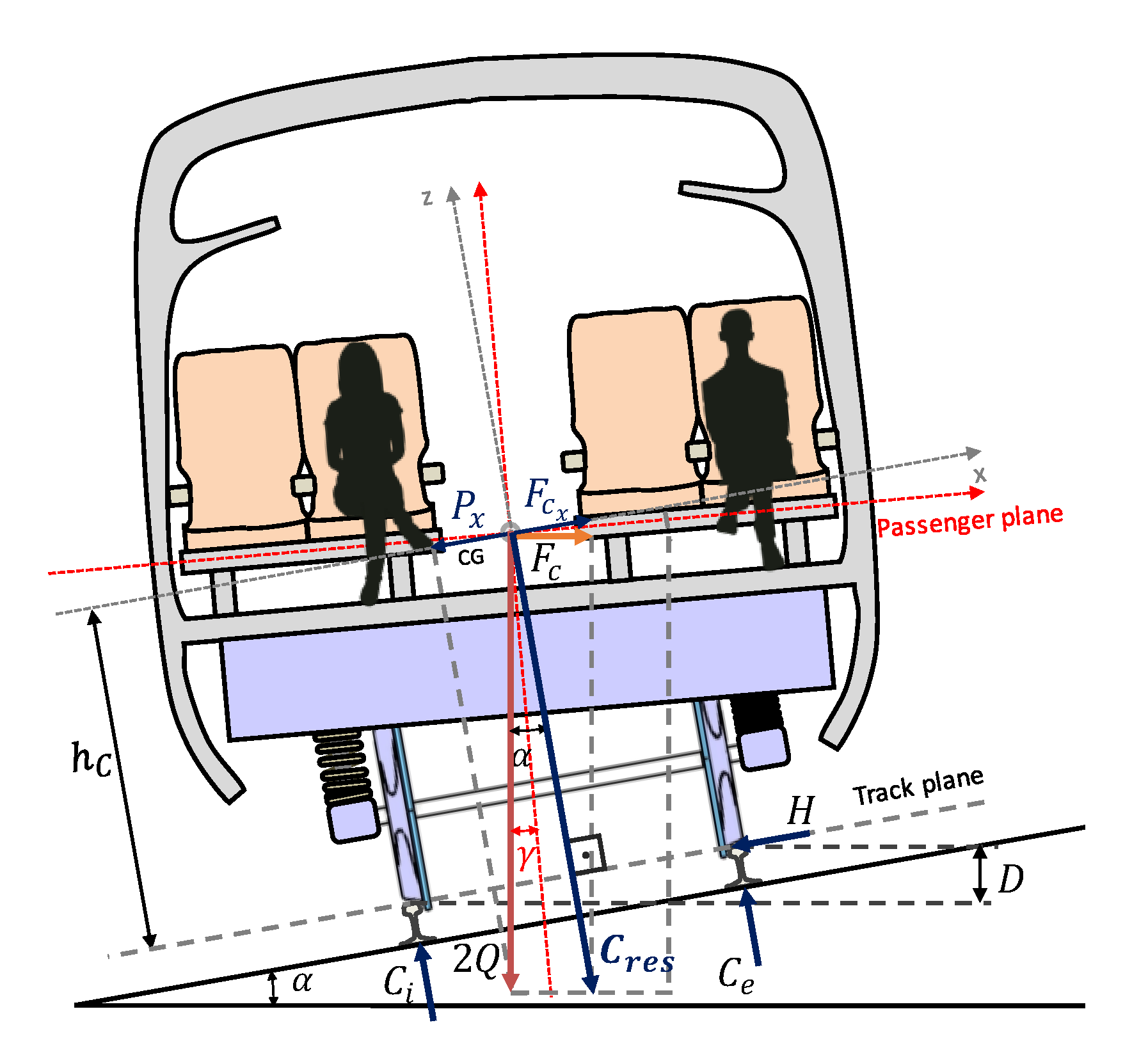
Figure 1. Equilibrium cant.
Sustainability 14 08377 g001
Figure 2. Definition of cant deficiency (I).
Sustainability 14 08377 g002
Figure 3. Accelerations acting in a vehicle circulating in a curve.
Sustainability 14 08377 g003
Figure 4. Graphic representing the design radii as a function of the cant criterion.
Sustainability 14 08377 g004
Figure 5. Comparison criteria for all types of trains in the graphical method.
Sustainability 14 08377 g005aSustainability 14 08377 g005b
Figure 6. Transition curve design graph.
Sustainability 14 08377 g006
Figure 7. Location of the case study (Adif) [33].
Sustainability 14 08377 g007
Figure 8. Case study sections (Adif [33]).
Sustainability 14 08377 g008
Figure 9. Graphic design curves for Alternative 1 using an alpha method with α = 6.2.
Sustainability 14 08377 g009
Figure 10. Graphic design curves for Alternative 2 using 2/3 of the equilibrium cant method.
Sustainability 14 08377 g010
Figure 11. Graphic design curves for Alternative 3 using an alpha method with α = 6.66.
Sustainability 14 08377 g011
Figure 12. Graphic design curves for Alternative 4 using the Modified Root Mean Square method.
Sustainability 14 08377 g012
Figure 13. Comparison of tracks between alternatives.
Sustainability 14 08377 g013
Figure 14. Comparison in a curve between alternatives.
Sustainability 14 08377 g014
Table 4. Limits for design parameters established by several technical standards for railway track design.
StandardTraffic TypeGauge
(mm)
Vmax
(km/h)
D max
(mm)
I m a x
(mm)
Emax
(mm)
dD/dt
(mm/s)
dD/dl
(mm/m)
a v m a x
(m/s2)
FranceMSRs
HSRs
1435≤250
≥300
160
180
150
100
70–100300.5–0.71–2
GermanyHSRs1435≥30018015070–110300.5–0.71–2
SpainMSRs
HSRs
1435250
350
14060
80
905010.52
0.39
SwedenHSRs
F
1435300
120
100150
100
10055
46
-0.98
0.43
BelarusMSRs1520140150115--0.50.7
LatviaP + F1435250 + (120)9010090302.51
LithuaniaP + F1435250 + (120)9010090302.51
RussiaMSRs1520140150115--0.50.7
SlovakiaMSRs1520200150115--0.50.7
UkraineMSRs1520140150115--0.50.7
EstoniaP + F1435250 + (120)9010090302.51
PolandMSRs1520200150100-30-0.7
USAHSRs
F
1435300
120
15076
50
---0.9–1.2
JapanHSRs1435500200-----
TSIHSRs1435300180–1908011060--
CENHSRs143530018010011060--
Table 5. Characteristics of all types of trains (Renfe) [32].
Type of TrainCharacteristicValue
High-speed train
Talgo T350
(S-102 class)
4 circulations/way
# Cars12
V 1 m a x   km / h 350
s−0.3
hc (m)1.2
# Axles21
Weight per axle (Tn/axle)16
Shuttle train (S-114 class)
10 circulations/way
# Cars4
V 2 m a x   km / h 250
s0.2
hc (m)1.5
# Axles16
Weight per axle (Tn/axle)17
Freight train
5 circulations/way
# Wagons35
V 3 m a x   km / h 100
hc (m)1.5
# Axles140
Weight per axle (Tn/axle)20
Table 7. Estimated demand following Adif [33] and traffic forecasts.
YearServiceEstimated Demand# Trains Each Way
2030AVE Madrid–Lisbon2,022,050 passengers/year15
Avant Madrid–Talavera399,646 passengers/year4
Freight-8
2050AVE Madrid–Lisbon2,471,893 passengers/year18
Avant Madrid–Talavera488,555 passengers/year5
Freight-10
Publisher’s Note: MDPI stays neutral with regard to jurisdictional claims in published maps and institutional affiliations.