Using a Novel Algorithm Based on the Random Vector Functional Link Network and Multi-Verse Optimizer to Forecast Effluent Quality

Abstract

The treatment of wastewater is a complicated biological reaction process. Reliable effluent prediction is critical in the scientific management of water treatment plants. This research proposes a soft sensor design strategy to address the issues above, Multi-Verse Optimizer (MVO)-based random vector functional link network (MVO-RVFL). The proposed approach is utilized to anticipate real-time effluent data obtained from the Benchmark Simulation Model 1 (BSM1). The results of the experiments demonstrate that the MVO methodology can successfully find the optimum input-hidden weights and hidden biases of the RVFL model while outperforming the original RVFL and other typical machine learning approaches in all types of influent datasets. In the situation of significant water quality variations, the use of the fusion process for model development was also investigated. The experimental results demonstrate that incorporating prior knowledge can effectively improve the model’s ability to cope with unexpected situations.

1. Introduction

The pollution of water resources has become a major environmental problem in the world today [1,2]. As a vital part of water resource protection, the wastewater treatment process must be controlled to maintain the effluent standards [3]. However, the water treatment system is a hysteretic, nonlinear system that usually involves a series of chemical reactions [4]. Conventional water treatment processes include membrane filtration technologies, Fenton oxidation processes, activated carbon-mediated adsorption, photocatalysis, and electrochemical oxidation [5]. Advanced treatment technologies include bioelectrical systems [6], advanced oxidation process [7], and enzymatic treatment [8], which are mainly in the research phase. A significant requirement for quality assurance of water treatment is real-time monitoring of crucial availability indicators. Unfortunately, some of these indicators are difficult to detect in real-time and effectively [9]. For example, BOD₅ can only be obtained through laboratory tests and takes five days, which makes it challenging to meet the requirements for real-time monitoring [10]. Despite the fact that the development of sensor technology for water quality control and monitoring was motivated by challenges in the rapid and accurate identification of pollutants, it still faces issues such as sensitivity, stability and selectivity, high cost, and no control over interferents/effect of counter ions [11]. To address these issues, soft measurement methods are widely used to accomplish real-time measurements of several variables.

Soft measurement refers to a set of techniques that make use of tolerance for error and uncertainty in order to gain tractability, resilience, and cheap solution costs [12,13]. The development of soft measuring techniques has benefited from the introduction of several machine learning algorithms in recent years and has performed well in the wastewater treatment sector [14]. Fuzzy modeling techniques are commonly employed in activated sludge processes. Ting et al. effectively eliminate the complex nonlinear variables present in Activated Sludge Model No.1 (ASM1) by combining the well-known fuzzy c-means cluster algorithm with the method of least squares [15]. The efficacy of this strategy, on the other hand, is strongly reliant on expert knowledge. Additionally, artificial neural networks (ANN) are among the most widely used soft sensing models today. Golzar, F. et al. [16] first apply an artificial neural network to the soft wastewater treatment plant to predict the temperature of the effluent; it simply employs publicly available historical data, with no field measurements required for complex heat transfer models. A soft sensor approach based on radial basis function neural networks was developed by Bagheri et al. to measure total phosphorus (TP), COD, and suspended solids (SS) [17]. However, there are significant downsides to gradient-based artificial neural networks, including overfitting, extended training times, and local minimum [18]. Random vector functional-link (RVFL) networks published by Y.-H. Pao in the 1990s is one technique for addressing this difficulty [19]. Instead of adjusting weights based on the back-propagation of gradients, RVFL sets weights by Moore–Penrose generalized inverse. This approach makes it possible to learn faster than traditional neural networks with guaranteed learning accuracy. Due to the characteristics described above, standard RVFL has been widely used in applications such as multiclass classification, image quality assessment, and human action recognition. Simultaneously, theories and algorithms relating to RVFL for particular applications have been enhanced. For example, RVFL was integrated with statistical hypothesis testing and self-organization of a number of enhancement nodes in Ref. [20], resulting in a novel learning system for remote sensing applications dubbed a statistical self-organizing learning system (SSOLS). In Ref. [21], an unsupervised parameter learning technique for RVFL, i.e., a sparse pre-trained random vector functional link (SP-RVFL) network, was proposed to adaptively discover better network parameters for particular learning tasks. In Ref. [22], RVFL was coupled with Adaboost in the pedestrian detection system.

Although water quality forecast accuracy is increasing, since water quality is inherently unstable and nonlinear in time series, more precise prediction approaches are worthy of further study. Technically, the use of standard RVFL nets suffers from design issues such as how to assign the random weights and bias. For the first time, a Multi-Verse Optimizer (MVO) is used as an alternative to solve the problem by optimizing the RVFL parameters based on the current successful implementations. Each solution to the goal issue is seen as a verse in MVO, with objective values evaluating performance. With the help of the relevant cosmological rules, they can gradually converge to the optimal position in the search space. The MVO approach is then utilized to estimate the RVFL model’s computing parameters, resulting in an innovative new hydrological forecast method. The suggested approach is used to anticipate BOD₅ and COD in the process of wastewater treatment. Our experiments are based on the BMS1 simulation platform. Compared to basic RVFL approaches and other standard machine learning algorithms, the findings demonstrate superior prediction accuracy and generalization capabilities.

Furthermore, the data-driven modeling technique is basically a black-box modeling approach, with the accuracy of models built without previous information and systematic mechanisms being restricted. According to preliminary findings, Cote et al. employed hybrid models comprising a modified ASM1 model and FFNN models to accurately predict the concentrations of SS, COD, and NH₄ in the effluent, DO in the bioreactor, and SS in the return sludge [23]. Lee et al. used a variety of PLS and ANN approaches to integrate a phenomenological model based on ASM1 and process knowledge. As a consequence, they suggested using a hybrid NNPLS model to get the most accurate forecast results while simultaneously identifying and isolating process problems [24]. The evidence in the publications indicates that hybrid models are more accurate. At the end of the experiment, we attempt to extract the relationship between the data better with the help of some systematic mechanisms and a priori knowledge to obtain more accurate modeling and prediction results.

To be summarized, the study’s novelty for both the computer science and hydrological sectors comes in three aspects: (1) For the first time, the MVO approach is employed to calculate RVFL computation parameters and improve the network performance. (2) We demonstrate our approach on BSM1 and show its great predictive accuracy by predicting BOD5 and COD, which are difficult to measure directly. (3) We use mechanistic information from the biological treatment of water to build new model features and explore their validity.

The rest of this paper is organized as below: the underlying theory and the computational process of the model are described in Section 2. The proposed MVO-RVFL-based soft measurement approach is given in Section 3. The simulations and experiment results are shown in Section 4, while the conclusions are given at the end.

2. Prediction Model Principle

2.1. Theory

RVFL is an algorithm for solving single hidden layer neural networks. Its most essential characteristic is that it can randomly initialize input weights and biases and acquire the appropriate output weights, making it quicker than standard learning algorithms while maintaining learning accuracy.

Suppose there are N training samples with n dimensions.

$$T=\left\{\left(X_i,t_i\right)X_iϵR,t_iϵR\right\}$$

(1)

$$X_i={\left[x_{i1},x_{i2},\dots ,x_{in}\right]}^T$$

(2)

$$t_i={\left[t_{i1},t_{i2},\dots t_{im}\right]}^T$$

(3)

A single hidden layer neural network with L hidden layer nodes can be expressed as:

$${\displaystyle \sum }_{i=1}^L{\beta }_{i}g\left(W_i\cdot X_j+b_i\right)+{\displaystyle \sum }_{i=L+1}^{L+n}{\beta }_i{X}_j=o_j, j=1,\dots ,N$$

(4)

where g( ) represents the activation function, W_i represents the weights between hidden nodes and input, b_i represents the bias vector of hidden layer neurons, and β_i represents the weights between the hidden nodes and output.

The goal of the single hidden layer neural network learning is to minimize the error between the output and actual value, which can be expressed as:

$${\displaystyle \sum }_{i=1}^N||o_j-t_j||=0$$

(5)

The above equation can be expressed in a matrix as:

$$H\beta =T$$

(6)

$$H={\left[\begin{array}{cccccc}g\left(W_1{X}_1+b_1\right)& \cdots & g\left(W_L{X}_1+b_L\right)& x_{11}& \cdots & x_{1d}\\ ⋮& \ddots & ⋮& ⋮& \ddots & ⋮\\ g\left(W_1{X}_N+b_1\right)& \cdots & g\left(W_L{X}_N+b_L\right)& x_{N1}& \cdots & x_{Nd}\end{array}\right]}_{N\times \left(L+d\right)}$$

(7)

$$\beta ={\left[\begin{array}{c}{\beta }_1^T\\ \cdot \\ \cdot \\ \cdot \\ {\beta }_L^T\end{array}\right]}_{\left(L+d\right)\times M}$$

(8)

$$T={\left[\begin{array}{c}{T}_1^T\\ \cdot \\ \cdot \\ \dot{T_N^T}\end{array}\right]}_{N\times M}$$

(9)

Gradient descent learning algorithms require all parameters to be adjusted in the iterative process. In the RVFL algorithm, once the input weights and the bias of the hidden layer are determined randomly, the output matrix of the hidden layer β is determined. The formula can calculate β:

$$\beta ={\left(H^{T}H\right)}^{-1}{H}^{T}T$$

(10)

The RVFL calculation process can be summarized as follows:

(1)

Initialization, given the number of hidden layer nodes L and the activation function g( );

(2)

Randomly generated W and b;

(3)

Calculate the output matrix H;

(4)

Calculate β using the Formula (10).

2.2. Subsection

Inspired by the multiverse theory in physics, S Mirjalili et al. [25] introduced the Multi-Verse Optimizer, a revolutionary swarm intelligence optimization technique. The MVO algorithm simulates the motion of the multiverse population under the combined action of white holes, black holes, and wormholes. The MVO algorithm follows the following rules in performing the optimization:

• If the expansion rate is higher, the higher the chance of producing a white hole. Conversely, if a universe has a relatively low expansion rate, it is more likely to make a black hole.
• White holes repel objects, and black holes absorb them.
• Irrespective of the expansion rate, it is possible for any other universe to transport objects to the current optimal universe through a wormhole.

Suppose there are n verses in the group.

$$U=\left[\begin{array}{c}{x}_1^1,x_1^2,\dots ,x_1^d\\ x_2^1,x_2^2,\dots ,x_2^d\\ \dots ,\dots \\ x_n^1,x_n^2,\dots ,x_n^d\end{array}\right]$$

(11)

where d is the number of variables, and n is the number of universes. Due to the different expansion rates of each respective universe, objects in individual universes are transferred through white hole/black hole orbits. This process follows the roulette wheel mechanism, as shown in Equation (12).

$$\begin{array}{c}{x}_i^j=\{\begin{array}{cc}{x}_k^j& r1<NI\left(U_i\right)\\ x_i^j& r1\ge NI\left(U_i\right)\end{array}\end{array}$$

(12)

where NI(U_i) represents the normalized expansion rate of the ith universe, and r1 is a random number in [0, 1]. In addition, the individual universe excites internal objects to move towards the current optimal universe to achieve local changes and improve its expansion rate. This process is executed according to Equation (13).

$$x_i^j=\{\begin{array}{c}\{\begin{array}{c}Xj+TDR\times (\left(u{b}_j-l{b}_j\right)\times r4+l{b}_j r3<0.5\\ Xj-TDR\times (\left(u{b}_j-l{b}_j\right)\times r4+l{b}_j r3\ge 0.5\end{array}\\ x_{i }^j r2\ge WEP\end{array}$$

(13)

where X_j indicates the jth parameter of the best universe formed so far, lb_j shows the lower bound of the jth variable, ub_j is the upper bound of the jth variable, and r2, r3, and r4 are random numbers in [0, 1]. WEP denotes the probability of the existence of wormholes in the multiverse, and TDR indicates the step size of an object moving towards the current optimal universe. The principle of renewal for WEP and TDR is based on Equations (14) and (15).

$$WEP=WE{P}_{min}+l\times \left(\frac{WE{P}_{max}-WE{P}_{min}}{L}\right)$$

(14)

$$TDR=1-\frac{l^{\frac{1}{p}}}{L^{\frac{1}{p}}}$$

(15)

3. Proposed Water Quality Forecasting System

The RVFL model’s assumption is stated in Section 2.1, and the input layer’s biases and weights are chosen at random in the RVFL model. With this method, the validity of the bias and weight values cannot be ensured, resulting in poor prediction stability for the RVFL model. Due to the inadequacies of the RVFL model, in MVO-RVFL, the weight matrix connecting the input layer to the hidden layer and the bias vector of the hidden layer are both optimized. The MVO approach employs the interchange of matter between created verses to imitate the information sharing of schemes. Owing to the integrated adaptive WEP/TDR constants and wormholes coupled that help MVO to provide high exploitation. Superior exploration of the suggested technique is due to the white and black holes that enable universes to exchange various items; it implies that it is more probable to avoid local optima.

The detailed operation steps of MVO-RVFL are shown below:

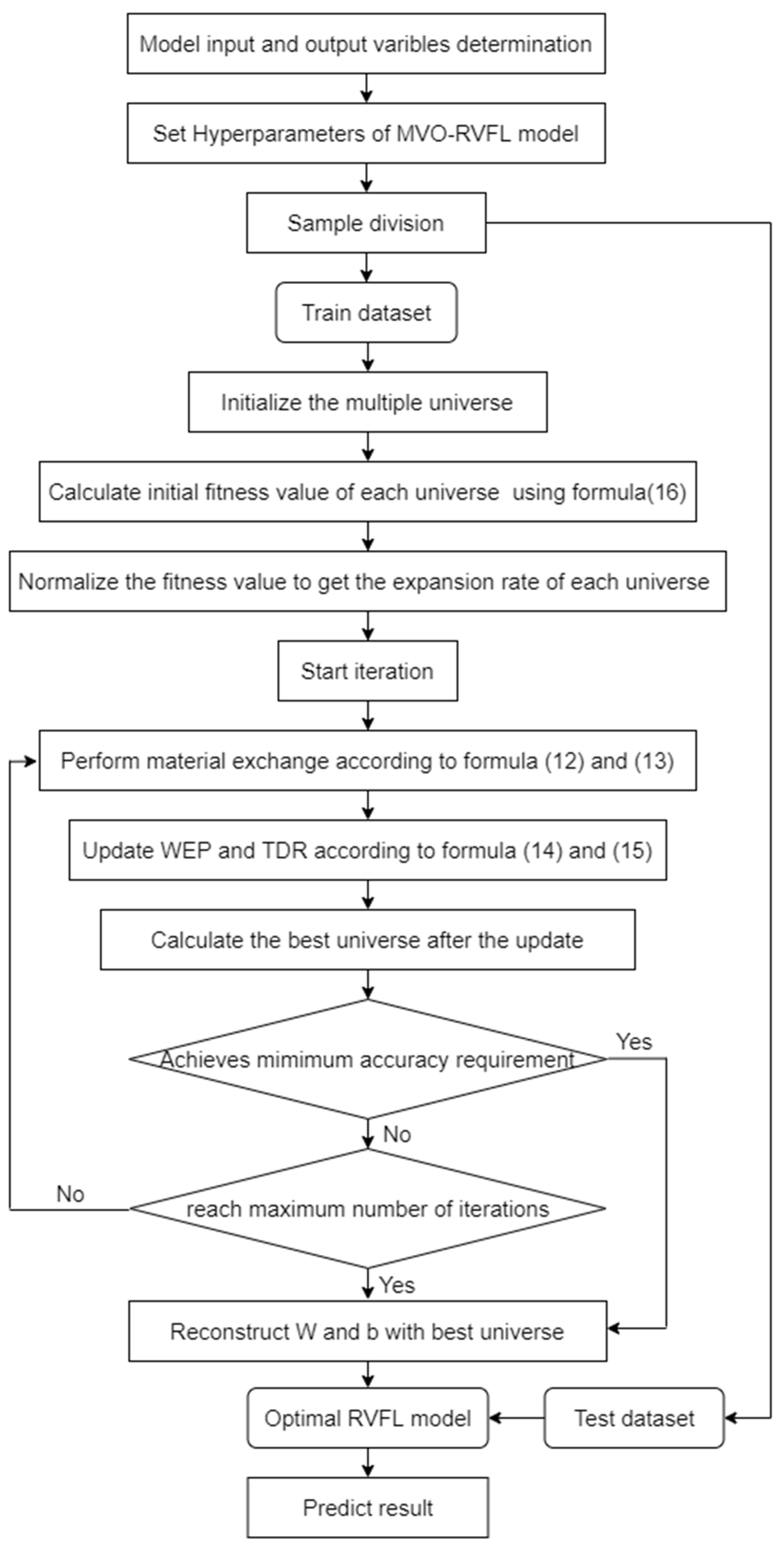
• Step 1: Set the model’s hyperparameters, such as WEPmin, WEPmax, exploitation p in MVO, the maximum number of iterations L, number of hidden neurons, and activation function in RVFL.
• Step 2: Set the root mean square error to the objective function, as shown in Formula (16) (The β_i in Formula (16) is calculated from Formulas (6)–(10)). It is used to compute the fitness value of each universe and sort them according to this.

  $$Fun{c}_{objective}=\sqrt{\frac{{{\displaystyle \sum }}_{j=1}^{N_{\mathrm{samples}}}{{\displaystyle \sum }}_{i=1}^m{\left({\beta }_i\times g\left(w_i\times x_j+b_i\right)-t_j\right)}^2}{m·N_{\mathrm{samples}}}}$$

  (16)
• Step 3: Start iteration. The RVFL parameters are optimized using the MVO approach.
  • Step 3.1: Initialize each universe with a random function. Each universe is a vector, and the dimension can be calculated by Formula (17) since it stands for W and b.

    $$dimension=\left(L+1\right)\cdot m$$

    (17)
  • Step 3.2: Perform material exchange according to Formulas (12) and (13). Calculate the best universe after the update.
  • Step 3.3: Calculate the fitness value of all the universes at the current cycle by Formula (16)
• Step 4: Determine if one of the objective conditions (1. Complete the maximum number of iterations; 2. Achieves minimum accuracy requirements) is met. If the specified criterion is satisfied, go to the next step. If not, proceed with the iteration process.
• Step 5: Divide the best universe’s vector into two parts: W and b; calculate the output matrix of the hidden layer β by Formula (10), then the optimal RVFL is obtained. MVO-RVFL has the obvious problem of requiring all intelligence to be traversed before finishing a single loop. The time investment is worthwhile, however, because influent data from the wastewater treatment process might change quickly and abruptly. As a result, slipping into a local optimum too soon will result in massive deviations.

Figure 1 shows the flow chart of effluent quality forecasting.

4. Wastewater Data and Effluent Quality Prediction Result

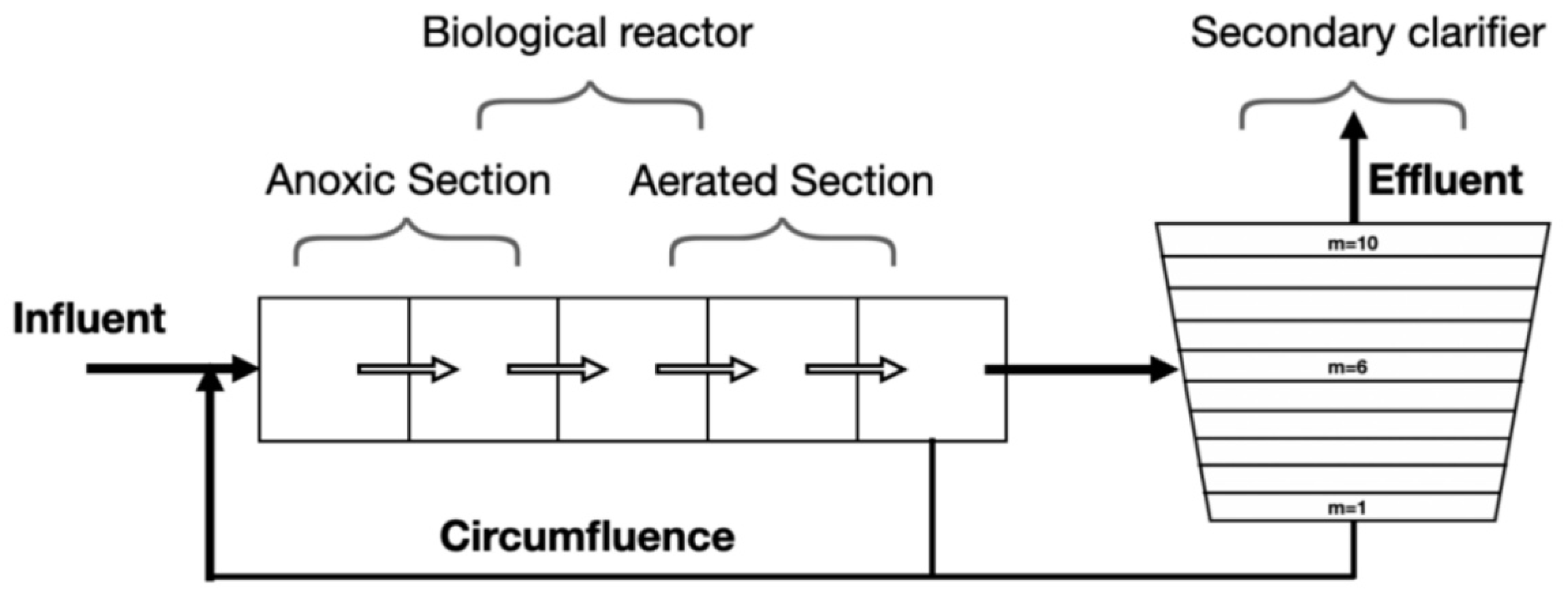
4.1. Description of BSM1 Benchmark Simulation Model 1 (BSM1)

Wastewater treatment plants (WWTPs) are massive nonlinear systems that are subjected to considerable changes in influent flow rate and pollutant load, as well as uncertainty about the composition of the entering wastewater. To judge the influence of different control strategies on reported plant performance as fair as possible, the Benchmark Simulation Model 1 (BSM1) was proposed by the European Scientific and Technical Cooperation Organization [26].

Two anoxic tanks and three aerobic tanks make up the benchmark plant’s five-compartment activated sludge reactor. In order to achieve biological nitrogen removal in full-scale plants, the plant combines nitrification and denitrification in a regularly utilized design. The activated sludge reactor is followed by a secondary clarifier. Approximately one-third of it is sent to the sixth layer of the secondary sedimentation tank, and the remaining third is redirected to unit one of the bioreactor. The majority of water that fulfills the discharge criteria is released from the tenth floor after sedimentation in the secondary sedimentation tank. The remainder is likewise returned to the biological reaction tank’s first unit. The general overview of the BSM1 plant is shown in Figure 2.

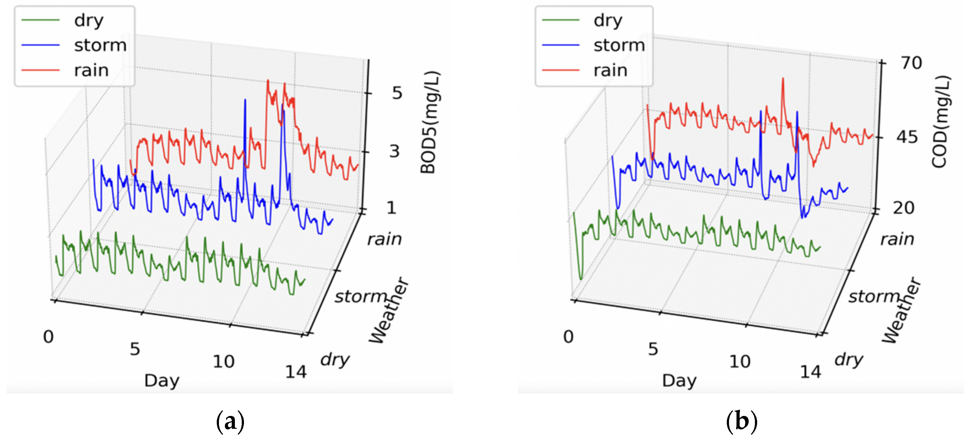
4.2. Data Acquisition through BSM1

This study selected the BSM1 built by Ulf Jeppsson et al. [23] in MATLAB/SIMULINK as a simulation platform. Influent datasets were provided by The International Water Association (IWA), including dry weather, storm weather, and rainy weather (Data and a more detailed description of BSM1 can be obtained under the link http://www.iea.lth.se/WWTmodels_download/, accessed on 21 May 2009). Each dataset comprises 14 days of influent data and 13 variables, with a sample interval of 15 min.

According to the flow sequence of wastewater in the reactor, the model of each unit is established in turn, which is composed of differential equations representing the reaction rates of the components. After inputting the supplied initial parameters, the model is simulated in a steady-state for 100 days. To verify the correctness of the model, the simulation outcomes must correspond with IWA’s steady-state results. After this, the simulation of dynamic water influent data can be carried out, and noise in measurements should be used together with the dynamic files. Due to the severe environmental hazards of BOD5 and COD and the fact that they are difficult to measure directly, they are used as the main effluent characteristics to study in this paper. The curves of both are shown in Figure 3 and are highly nonlinear. Additionally, the effluent fluctuates with the weather, resulting in different BOD5 and COD in different weather.

4.3. Preprocess and Model Parameter Settings

For the sample division, the amount of data in the trainset usually accounts for 66.67% to 80% of the total. Therefore, in this prediction process, the first 11 days of influent data were selected as input for model training, and the last three days of influent data were used as input for testing. For the reason that only So, Sno, Snh, and Salk are readily measurable through the laboratory or online instruments, the selected predictor variables are shown in

Table 1. Input features of the prediction model.

Definition	Notation
Influent Ammonia Concentration	Snh,in
Influent Flow Rate	Q,in
Nitrate and nitrite nitrogen (reactor 1)	Sno
Nitrate and nitrite nitrogen (reactor 2)	Sno
Dissolved Oxygen Concentration (reactor 3)	So
Dissolved Oxygen Concentration (reactor 4)	So
Dissolved Oxygen Concentration (reactor 5)	So
Total Suspended Solid (reactor 5)	TSS
Alkalinity	Salk
Oxygen Transfer Coefficient (reactor 5)	Kla5

. In terms of hidden layer node selection, the theory is that the more hidden nodes in the model, the lower the model’s error. Excess hidden nodes, on the other hand, would use computer resources without providing a substantial benefit; therefore, the number of hidden nodes should be chosen in accordance with the predicted power constraint. We picked the appropriate network hyperparameters with an acceptable performance from a large number of tests. In our experiment, the number of hidden layer nodes was 20, the universe number was set to 120, and the maximum number of iterations was 200 while creating the MVO-RVFL soft measurement model. The data were normalized using Formula (18) before model learning to remove the effect of different magnitudes of incoming sample features. We will continue to research the selection of the model’s architecture in the future.

$$X=\frac{X-X_{min}}{X_{max}-X_{min}}$$

(18)

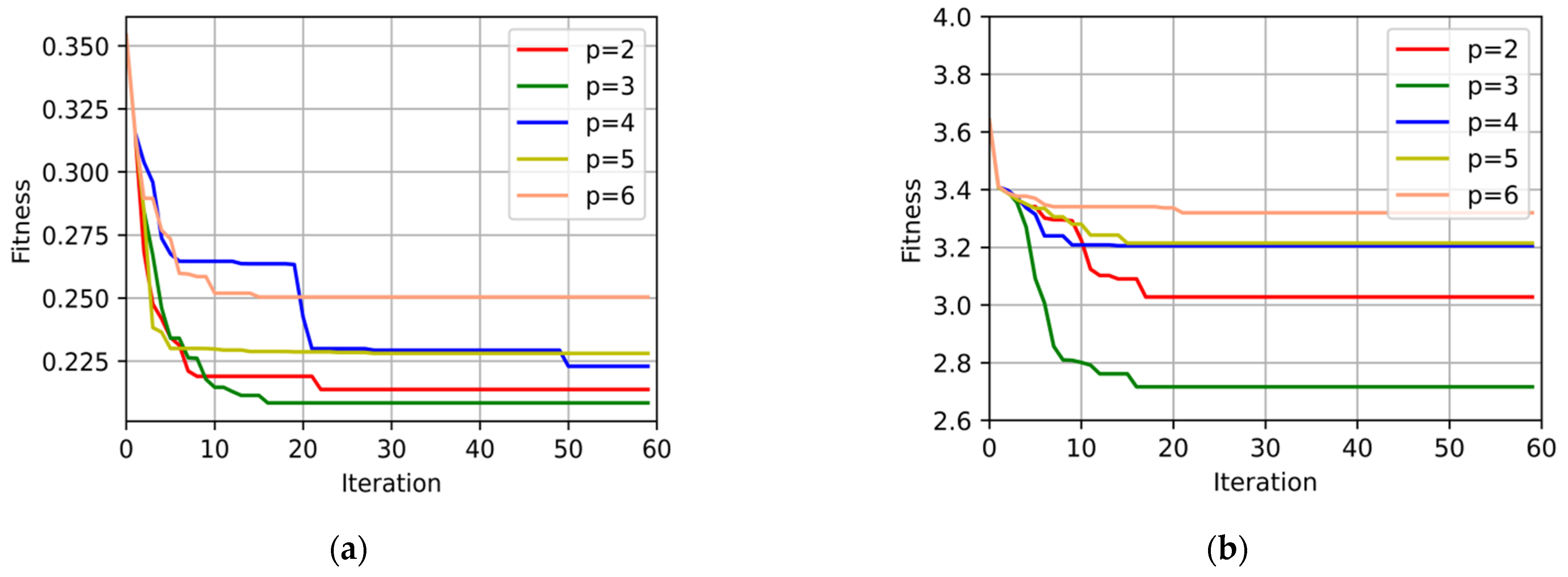
4.4. Exploitation and Exploration in the Iterative Process of MVO-RVFL

In Section 2.2, it is mentioned that the TDR denotes the distance at which an object transitions through a wormhole near the optimal universe. In the equation of TDR, p defines the detection speed that changes with the number of iterations; the higher the value of p, the faster the local detection speed and the shorter the time is taken. Figure 4 shows the rate of model iteration optimization for different values of p.

An appropriate p-value can save the amount of training time and have an excellent result. In Figure 4, it can be seen that as the p increases, the value of fitness convergence is higher, which means that the water quality prediction model is more likely to fall into a local optimum. This is consistent with the MVO theory that the higher the p-value, the faster the local detection speed and the shorter the time. However, in the water quality research, we are more concerned about the model’s accuracy, so we should try to avoid the local optimum. In fact, we can see that when p = 3, the fitness value of both models reaches the minimum and does not consume too many iterations. As a result of the trade-off, the parameter p is set to 0.3.

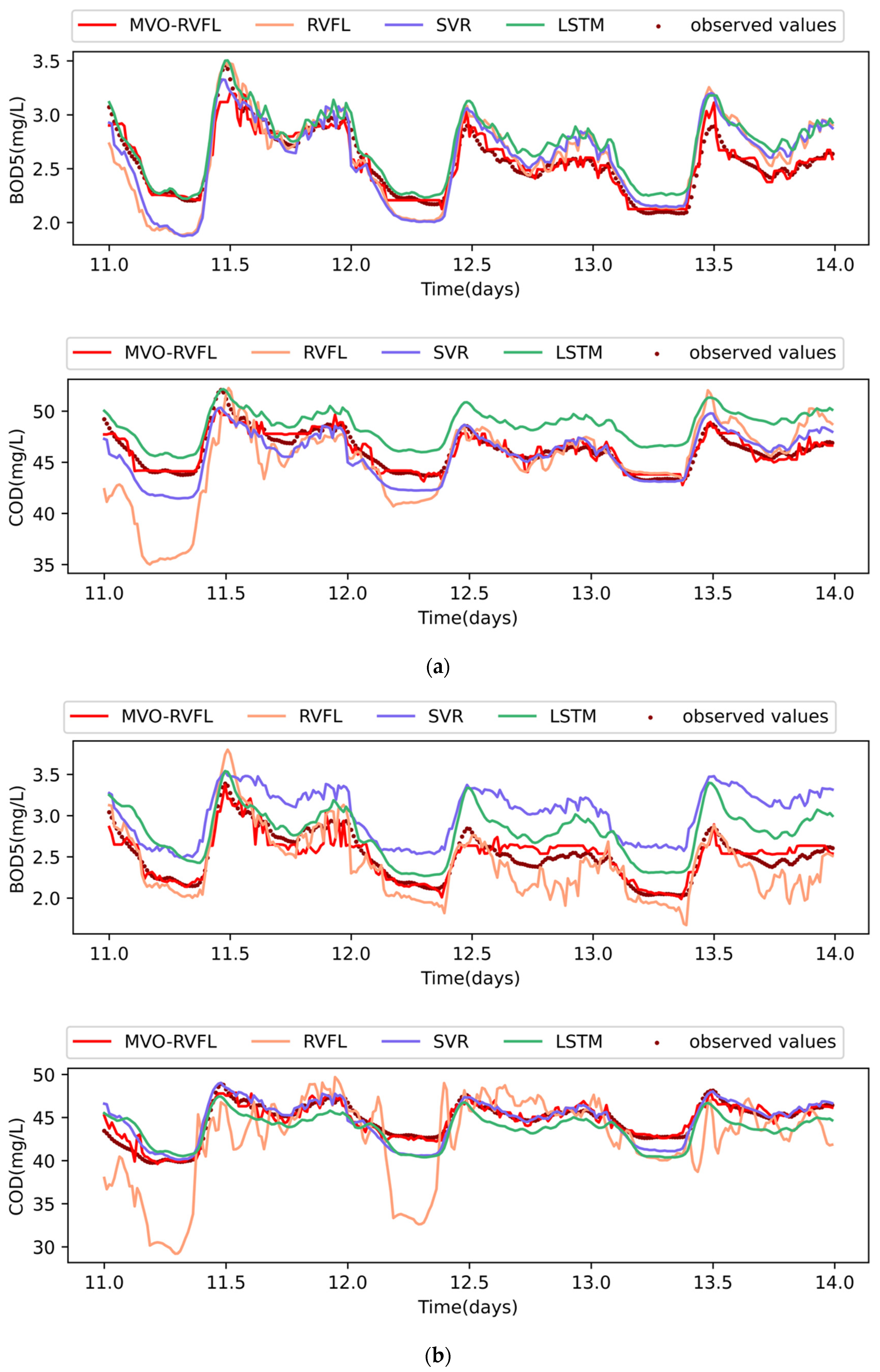
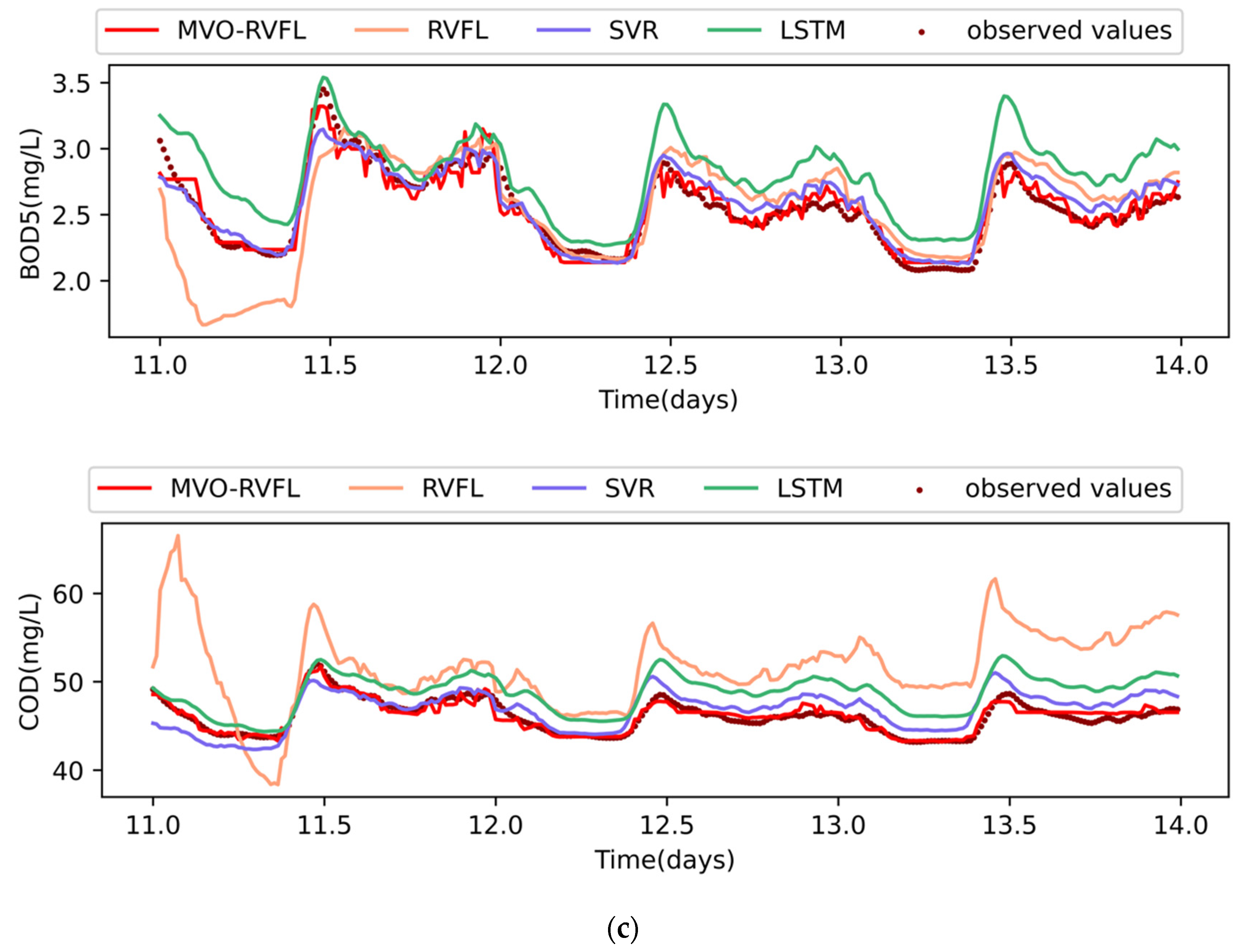
4.5. Experimental Results and Their Analysis

To test the effectiveness of the MVO-RVFL approach suggested in this study in predicting water quality, the original RVFL method, the conventional machine learning algorithm support vector regression algorithm (SVR), and long short-term memory (LSTM) were chosen for comparison. SVR is a common regression method, and LSTM is a state-of-the-art time series forecasting method. The results of the four prediction methods are shown in Figure 5, and it can be seen that the overall prediction effect of MVO-RVFL is better. The error between the predicted and actual values is demonstrated by the Root Mean Square Error (RMSE) in

Table 2. Evaluation of model prediction results.

Weather	Model	RSME of BOD5	RSME of COD
Dry	SVR	0.189	1.598
	LSTM	0.182	2.533
	RVFL	0.122	2.627
	MVO-RVFL	0.063	0.453
Rain	SVR	0.534	1.694
	LSTM	0.263	1.673
	RVFL	0.253	4.243
	MVO-RVFL	0.114	0.544
Storm	SVR	0.178	1.561
	LSTM	0.513	2.878
	RVFL	0.487	6.821
	MVO-RVFL	0.134	0.623

. In dry weather, compared to RVFL and another algorithm, the MVO-RVFL improves BOD5 prediction accuracy by at least 48.3% and COD prediction accuracy by at least 71.6%. On rainy days, BOD5 prediction accuracy improved by at least 54.9% and COD by 67.9%. In storm weather, the accuracy of BOD5 was raised by at least 24.7% and COD by 60.8% during the test phase. The rationale for the MVO-RVFL model’s superior performance is that it assigns appropriate random weights and biases, which is a major flaw in normal RVFL nets. In addition, it is worth noting that in weather with more fluctuating water quality, such as a storm, the prediction results produced by general prediction methods will be less accurate. In this case, MVO-RVFL can still guarantee a certain accuracy. This reflects the excellent global optimization ability of the MVO optimizer. Although MVO-RVFL will spend several times more time on model training, it is worthwhile to improve the accuracy.

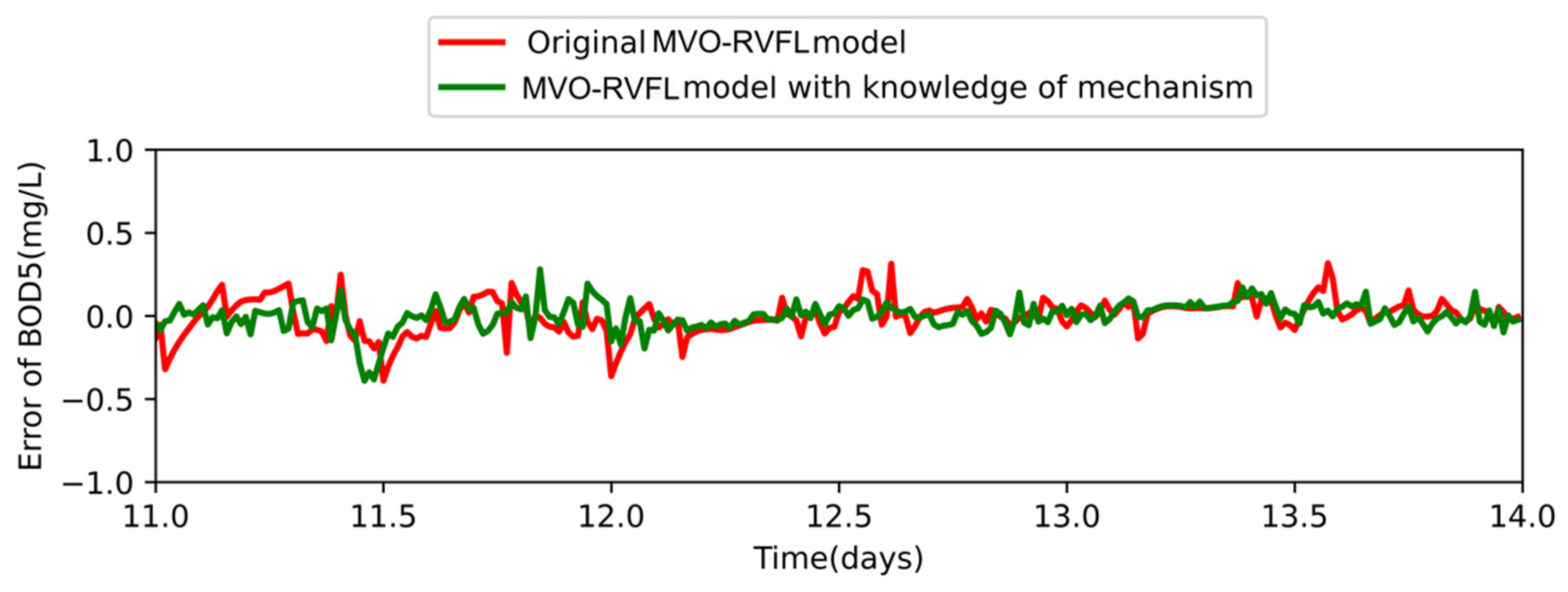
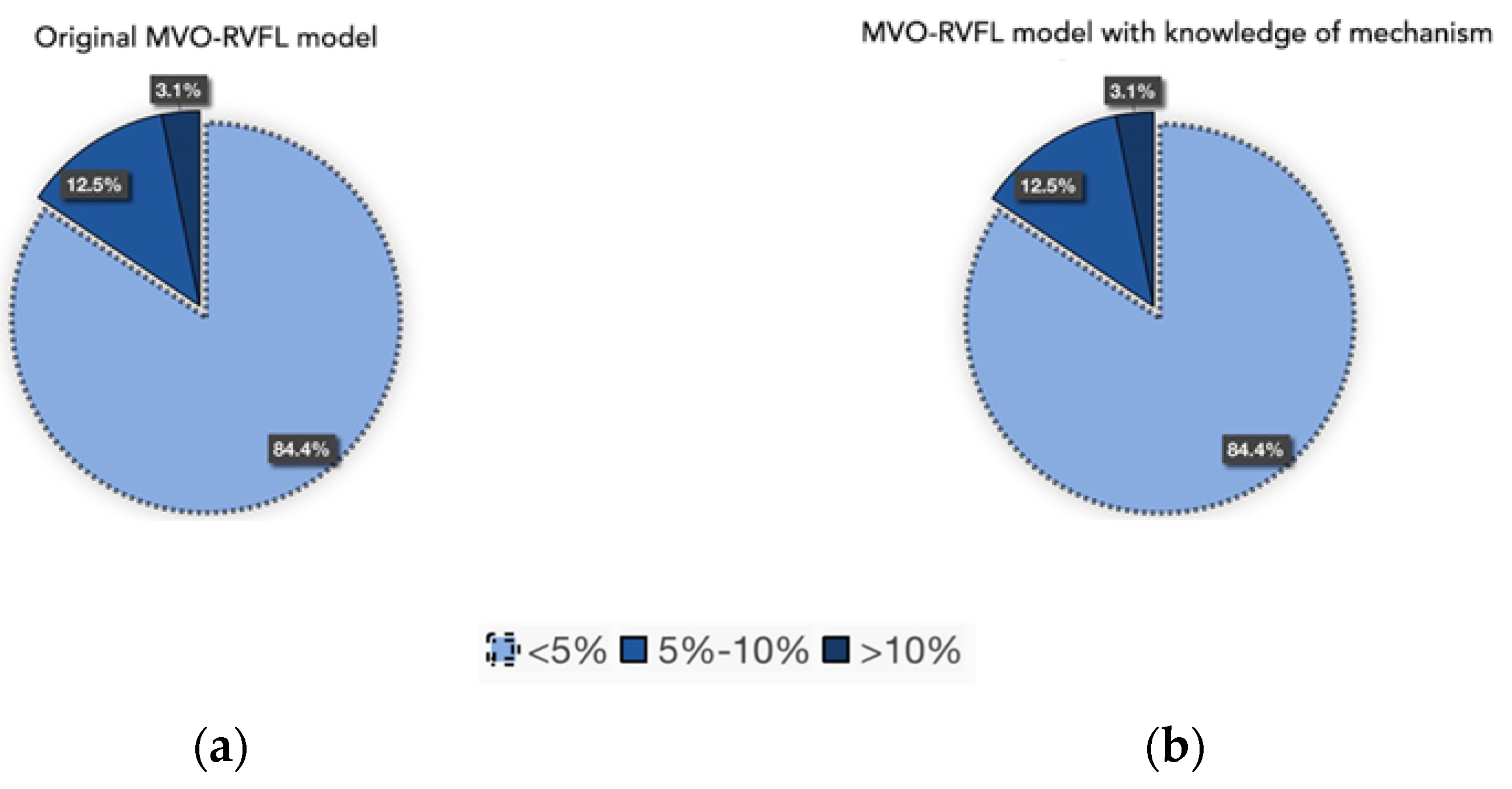
4.6. Study on the Validity of Hybrid Model

In the study of Section 4.4, we have noticed that the fluctuation trend of the influent data becomes more extensive, leading to a decrease in the prediction accuracy. Despite the fact that the MVO-RVFL model obtained more satisfactory forecasting results in each kind of weather, in storm weather, its own performance relative to dry and rain had a significant drop, which is embodied in the RSME increased by 1.18 times and 2.12 times, respectively.

Therefore, it is considered that the a priori knowledge obtained with the help of a mechanical model to extract the relationship between the data better achieved more accurate modeling and prediction results. In the mechanistic study of biological treatment methods for wastewater, there are equations proposed by Hiatt and Grady [27] that describe the rate of “Anoxic growth of heterotrophs ” and “Aerobic growth of autotrophs,” as shown in (18) and (19).

$${\rho }_1={\mu }_{\mathrm{H}}\left(\frac{S_{\mathrm{S}}}{K_{\mathrm{S}}+S_{\mathrm{S}}}\right)\left(\frac{K_{\mathrm{O},\mathrm{H}}}{K_{\mathrm{O},\mathrm{H}}+S_{\mathrm{O}}}\right)\left(\frac{S_{\mathrm{NO}}}{K_{\mathrm{NO}}+S_{\mathrm{NO}}}\right){\eta }_{\mathrm{g}}{X}_{\mathrm{B},\mathrm{H}}$$

(19)

$${\rho }_2={\mu }_{\mathrm{A}}\left(\frac{S_{\mathrm{NH}}}{K_{\mathrm{NH}}+S_{\mathrm{NH}}}\right)\left(\frac{S_{\mathrm{O}}}{K_{\mathrm{O},\mathrm{A}}+S_{\mathrm{O}}}\right)X_{\mathrm{B},\mathrm{A}}$$

(20)

Ss, Sno, and Snh are mentioned in Table 1, Xbh is the active heterotrophic biomass, Xba is the active autotrophic biomass, and the others are fixed kinetic parameters. The performance of the model is shown in Figure 6 and Figure 7.

As can be seen from Figure 6 and Figure 7, the model with knowledge of the mechanism performed better than the original MVO-RVFL model for the prediction of BOD5. In terms of model fit, the RSME of the model with knowledge of the mechanism is 0.090; compared to the original MVO-RVFL model, it is reduced by 32.8%. In terms of the distribution of errors, only 0.3% of the hybrid exceeded 10%, while the original MVO-RVFL model had 3.1%. This proves that mechanistic models do provide additional knowledge, and these are beneficial for model training.

Though with the help of new features, the model could better capture the nonlinear relationships among the variables. It is worth noting that the Xbh and Xba cannot yet be measured directly. We can acquire them in the simulation program in our experiment. In practice, however, they are calculated through indirect measurement and expert opinion. As a result, this strategy is likely to be used in the future.

5. Conclusions

In this paper, we propose an MVO-based variant of RVFL, MVO-RVFL. The MVO method optimizes the connection weights between the input and hidden layer neurons as well as the bias vector of the hidden layer, resulting in a more effective network. Using a population-based search technique, the MVO method creates many solutions at random from the problem space, then uses the exchange law of matter in the universe to repeatedly search for the optimal combination of parameters, therefore, increasing the search space and enhancing the quality of the findings.

The proposed model is used in wastewater treatment as a soft measurement. In terms of experimental prediction outcomes, the MVO-RVFL technique achieved the best degree of accuracy. It is worth mentioning that none of the predictive metrics under storm weather are as good or as accurate as other weather. As the number of raindrops increases, there are more unpredictability factors to consider, which makes accurate modeling more challenging. In this research, the mechanistic model information is included in the model’s feature building, hence reducing the complexity of the model training.

Due to time and effort limits, this research only makes a preliminary attempt to investigate the inclusion of this integrated data into the modeling process. The practicality of combining different sources of information in wastewater quality prediction tasks will be assessed in future studies.

References

1. Ming-qi, C. The Securing of Water Resource Issue and Its Nature. China Saf. Sci. J. 2009, 19, 17–22. [Google Scholar]
2. Skuras, D.; Tyllianakis, E. The perception of water related risks and the state of the water environment in the European Union. Water Res. 2018, 143, 198–208. [Google Scholar] [CrossRef] [PubMed]
3. Samuelssona, P.; Halvarsson, B.; Carlsson, B. Cost-efficient operation of a denitrifying activated sludge process. Water Res. 2007, 41, 2325–2332. [Google Scholar] [CrossRef]
4. Du, S. Modeling and control of biological wastewater treatment processes. Control. Theory Appl. 2002, 19, 660–666. [Google Scholar]
5. Ahmed, S.F.; Mofijur, M.; Nuzhat, S.; Chowdhury, A.T.; Rafa, N.; Uddin, M.A.; Inayat, A.; Mahlia, T.M.I.; Ong, H.C.; Chia, W.Y.; et al. Recent developments in physical, biological, chemical, and hybrid treatment techniques for removing emerging contaminants from wastewater. J. Hazard. Mater. 2021, 416, 125912. [Google Scholar] [CrossRef]
6. Dey, R.; Maarisetty, D.; Baral, S.S. A comparative study of bioelectrochemical systems with established anaerobic/aerobic processes. Biomass Convers. Biorefinery 2022. [Google Scholar] [CrossRef]
7. Bermudez, L.A.; Pascual, J.M.; Martinez, M.D.M.; Capilla, J.M.P. Effectiveness of Advanced Oxidation Processes in Wastewater Treatment: State of the Art. Water 2021, 13, 2094. [Google Scholar] [CrossRef]
8. Kennes-Veiga, D.M.; Gonzalez-Gil, L.; Carballa, M.; Lema, J.M. Enzymatic cometabolic biotransformation of organic micropollutants in wastewater treatment plants: A review. Bioresour. Technol. 2022, 344, 126291. [Google Scholar] [CrossRef]
9. Sanchez, A.; Wade, M.; Katebi, M.R. A software platform for real-time control and monitoring of a wastewater treatment plant. Trans. Inst. Meas. Control. 2005, 27, 153–172. [Google Scholar] [CrossRef]
10. Kulys, J.; Kadziauskiene, K. Yeast Bod Sensor. Biotechnol. Bioeng. 1980, 22, 221–226. [Google Scholar] [CrossRef]
11. Yadav, A.; Indurkar, P.D. Gas Sensor Applications in Water Quality Monitoring and Maintenance. Water Conserv. Sci. Eng. 2021, 6, 175–190. [Google Scholar] [CrossRef]
12. Zhou, M.; Feng, Y.; Chen, Y. Application of Soft Measurement Technology in Wastewater Treatment Process. China Water Wastewater 2005, 21, 34–36. [Google Scholar]
13. Huang, M.Z.; Ma, Y.W.; Wan, J.Q.; Chen, X.H. A sensor-software based on a genetic algorithm-based neural fuzzy system for modeling and simulating a wastewater treatment process. Appl. Soft Comput. 2015, 27, 1–10. [Google Scholar] [CrossRef]
14. Bagheri, M.; Akbari, A.; Mirbagheri, S.A. Advanced control of membrane fouling in filtration systems using artificial intelligence and machine learning techniques: A critical review. Process Saf. Environ. Prot. 2019, 123, 229–252. [Google Scholar] [CrossRef]
15. Yang, T.; Zhang, L.X.; Wang, A.J.; Gao, H.J. Fuzzy modeling approach to predictions of chemical oxygen demand in activated sludge processes. Inf. Sci. 2013, 235, 55–64. [Google Scholar] [CrossRef]
16. Golzar, F.; Nilsson, D.; Martin, V. Forecasting Wastewater Temperature Based on Artificial Neural Network (ANN) Technique and Monte Carlo Sensitivity Analysis. Sustainability 2020, 12, 6386. [Google Scholar] [CrossRef]
17. Bagheri, M.; Mirbagheri, S.A.; Ehteshami, M.; Bagheri, Z. Modeling of a sequencing batch reactor treating municipal wastewater using multi-layer perceptron and radial basis function artificial neural networks. Process Saf. Environ. Prot. 2015, 93, 111–123. [Google Scholar] [CrossRef]
18. Cao, Y.Y.; Cao, Y.T.; Guo, Z.Y.; Huang, T.W.; Wen, S.P. Global exponential synchronization of delayed memristive neural networks with reaction-diffusion terms. Neural Netw. 2020, 123, 70–81. [Google Scholar] [CrossRef] [PubMed]
19. Pao, Y.H.; Park, G.H.; Sobajic, D.J. Learning and Generalization Characteristics of the Random Vector Functional-Link Net. Neurocomputing 1994, 6, 163–180. [Google Scholar] [CrossRef]
20. Chi, H.M.; Ersoy, M.K. A statistical self-organizing learning system for remote sensing classification. IEEE Trans. Geosci. Remote Sens. 2005, 43, 1890–1900. [Google Scholar] [CrossRef]
21. Zhang, Y.S.; Wu, J.; Cai, Z.H.; Du, B.; Yu, P.S. An unsupervised parameter learning model for RVFL neural network. Neural Netw. 2019, 112, 85–97. [Google Scholar] [CrossRef]
22. Wang, Z.H.; Yoon, S.; Xie, S.J.; Lu, Y.; Park, D.S. A High Accuracy Pedestrian Detection System Combining a Cascade AdaBoost Detector and Random Vector Functional-Link Net. Sci. World J. 2014, 2014, 105089. [Google Scholar] [CrossRef]
23. Cote, M.; Grandjean, B.P.A.; Lessard, P.; Thibault, J. Dynamic Modeling of the Activated-Sludge Process—Improving Prediction Using Neural Networks. Water Res. 1995, 29, 995–1004. [Google Scholar] [CrossRef]
24. Lee, D.S.; Vanrolleghem, P.A.; Park, J.M. Parallel hybrid modeling methods for a full-scale cokes wastewater treatment plant. J. Biotechnol. 2005, 115, 317–328. [Google Scholar] [CrossRef] [PubMed]
25. Mirjalili, S.; Mirjalili, S.M.; Hatamlou, A. Multi-Verse Optimizer: A nature-inspired algorithm for global optimization. Neural Comput. Appl. 2015, 27, 495–513. [Google Scholar] [CrossRef]
26. Jeppsson, U.; Pons, M.N. The COST benchmark simulation model—Current state and future perspective. Control. Eng. Pract. 2004, 12, 299–304. [Google Scholar] [CrossRef]
27. Hiatt, W.C.; Grady, C.P.L., Jr. An Updated Process Model for Carbon Oxidation, Nitrification, and Denitrification. Water Environ. Res. 2008, 80, 2145–2156. [Google Scholar] [CrossRef]
Figure 1. Schematic diagram of the procedure.
Sustainability 14 08314 g001
Figure 2. General overview of the BSM1 plant.
Sustainability 14 08314 g002
Figure 3. Daily runoff data of three weather stations. (a) BOD5 curve of three kinds of weather, (b) COD curve of three kinds of weather.
Sustainability 14 08314 g003
Figure 4. Adaptation iterative process. Fitness is calculated by RSME in each episode. (a) BOD5 model; (b) COD model.
Sustainability 14 08314 g004
Figure 5. Comparison of prediction results based on three influential datasets. (a) Dry weather; (b) Rain weather; (c) Storm weather.
Sustainability 14 08314 g005aSustainability 14 08314 g005b
Figure 6. Comparison of BOD5 prediction errors before and after adding new features.
Sustainability 14 08314 g006
Figure 7. Distribution of errors over three intervals: 0–5%; 5–10%; 10–100%. (a) Original MVO-RVFL model; (b) MVO-RVFL model with knowledge of the mechanism.
Sustainability 14 08314 g007