
Assessment of Marine Debris on Hard-to-Reach Places Using Unmanned Aerial Vehicles and Segmentation Models Based on a Deep Learning Approach


Abstract
:1. Introduction
2. Methods
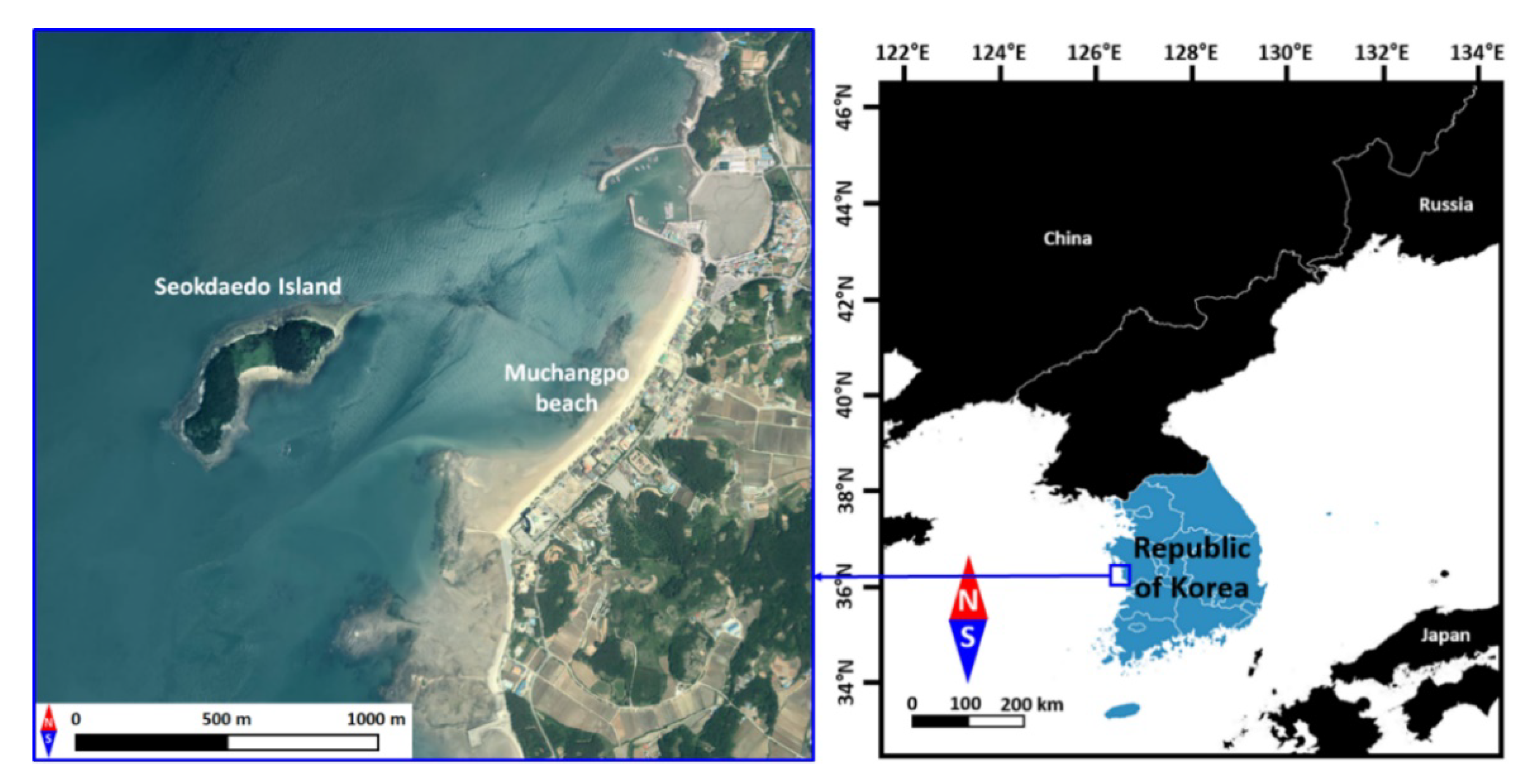
2.1. Study Area
2.2. Aerial Surveys Using Unmanned Aerial Vehicle (UAV)
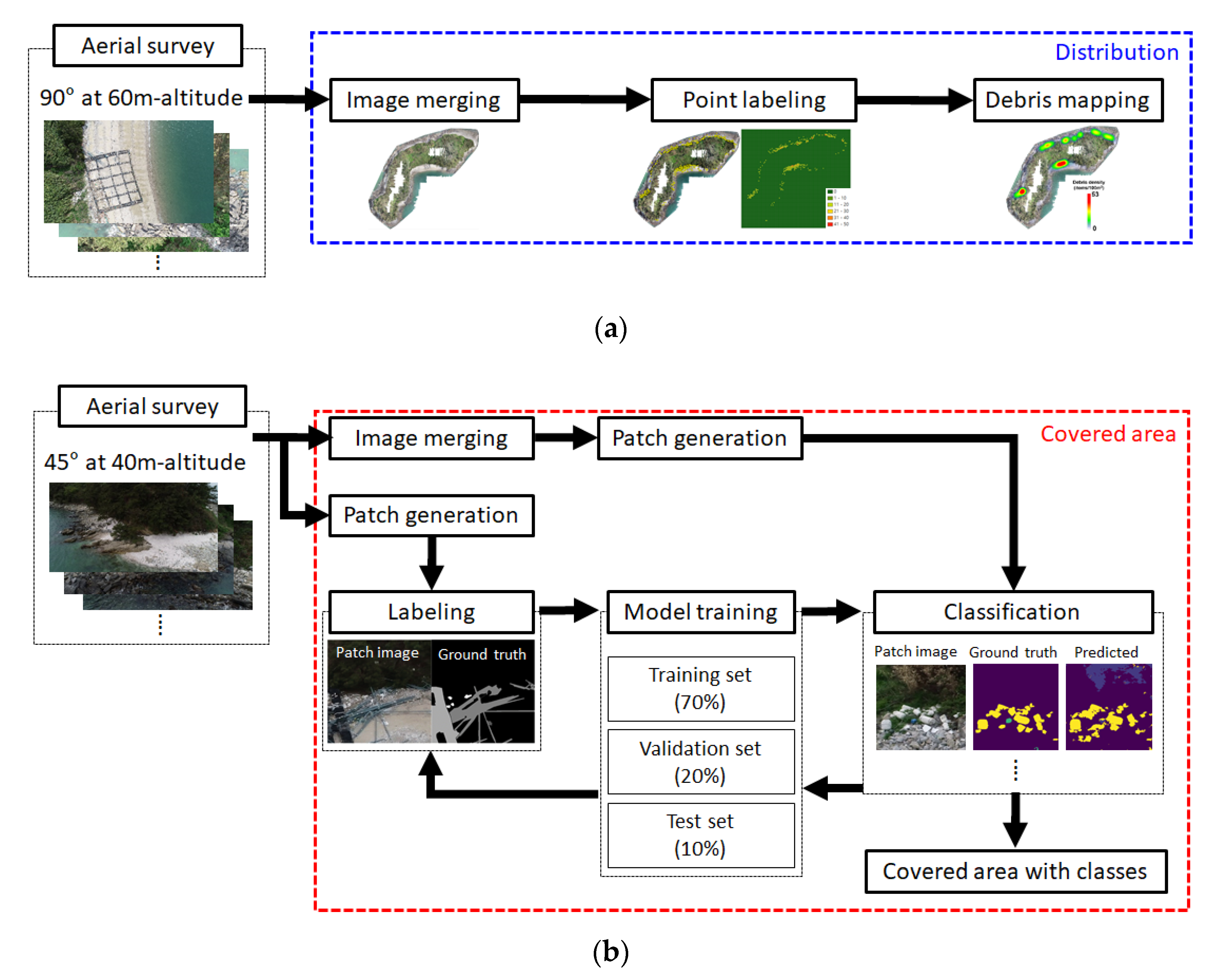
2.3. Workflows for Mapping and Classification of Coastal Debris
2.4. Model Performance
3. Results
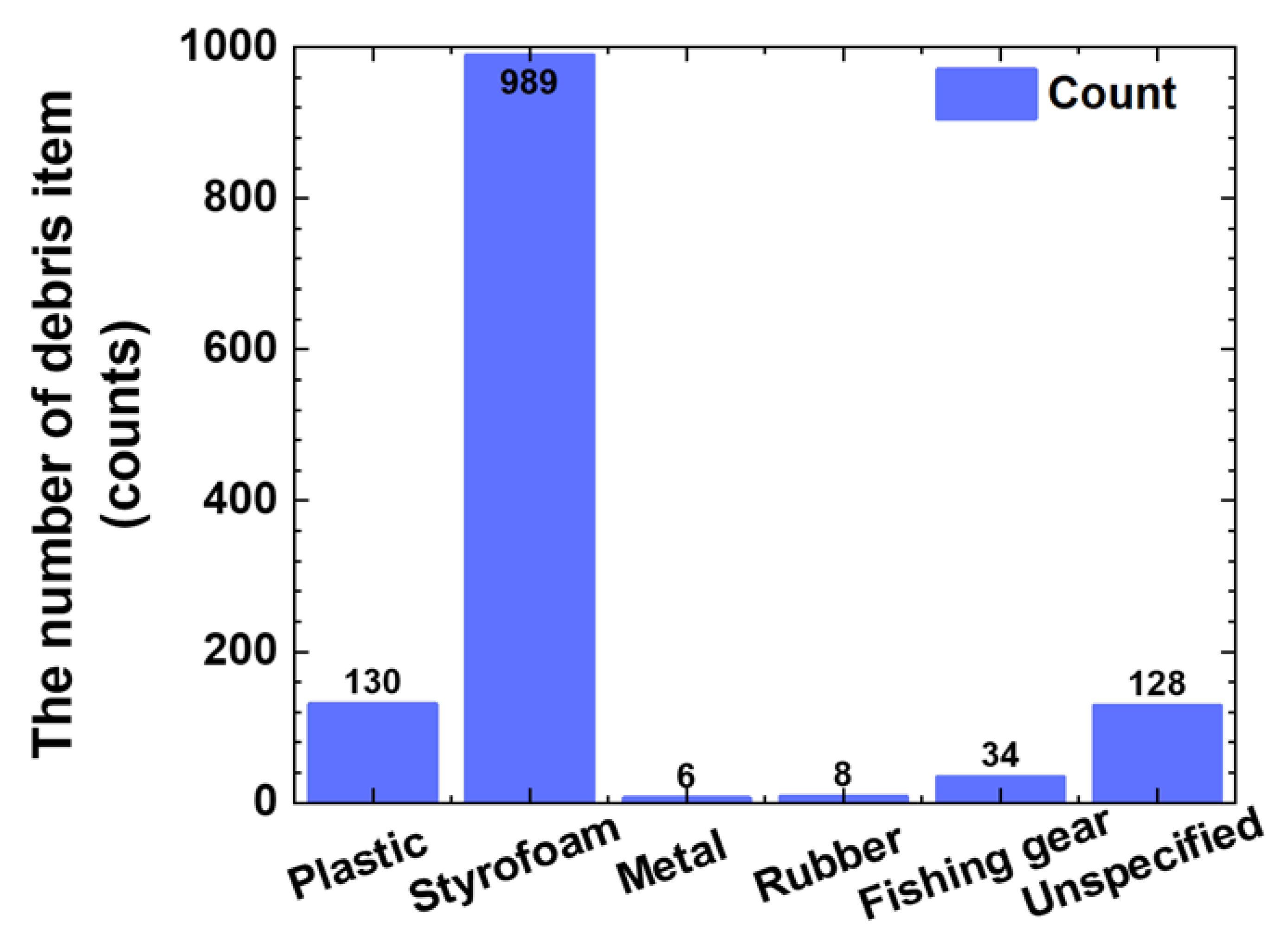
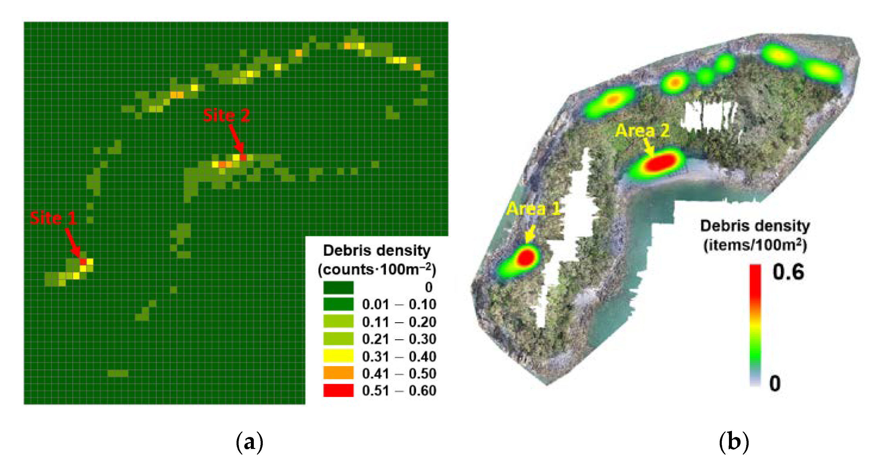
3.1. Coastal Debris Mapping
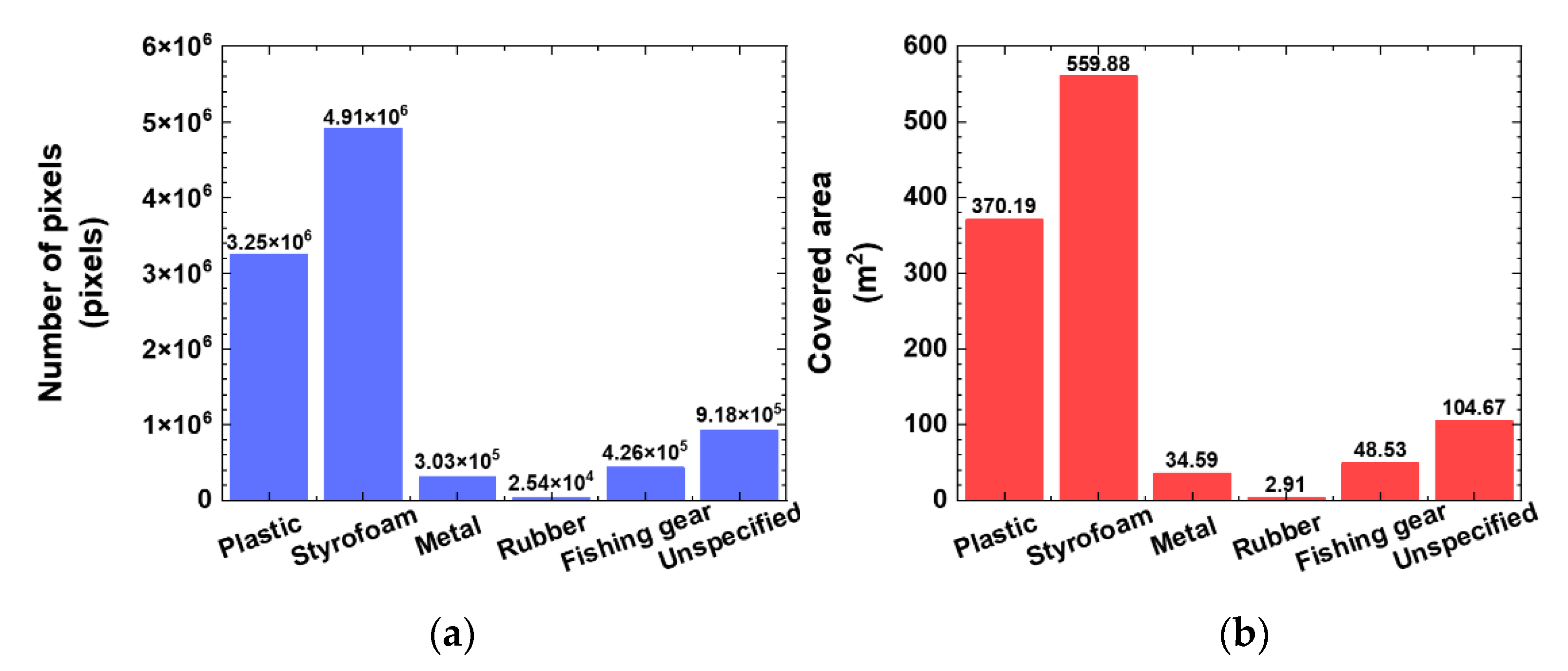
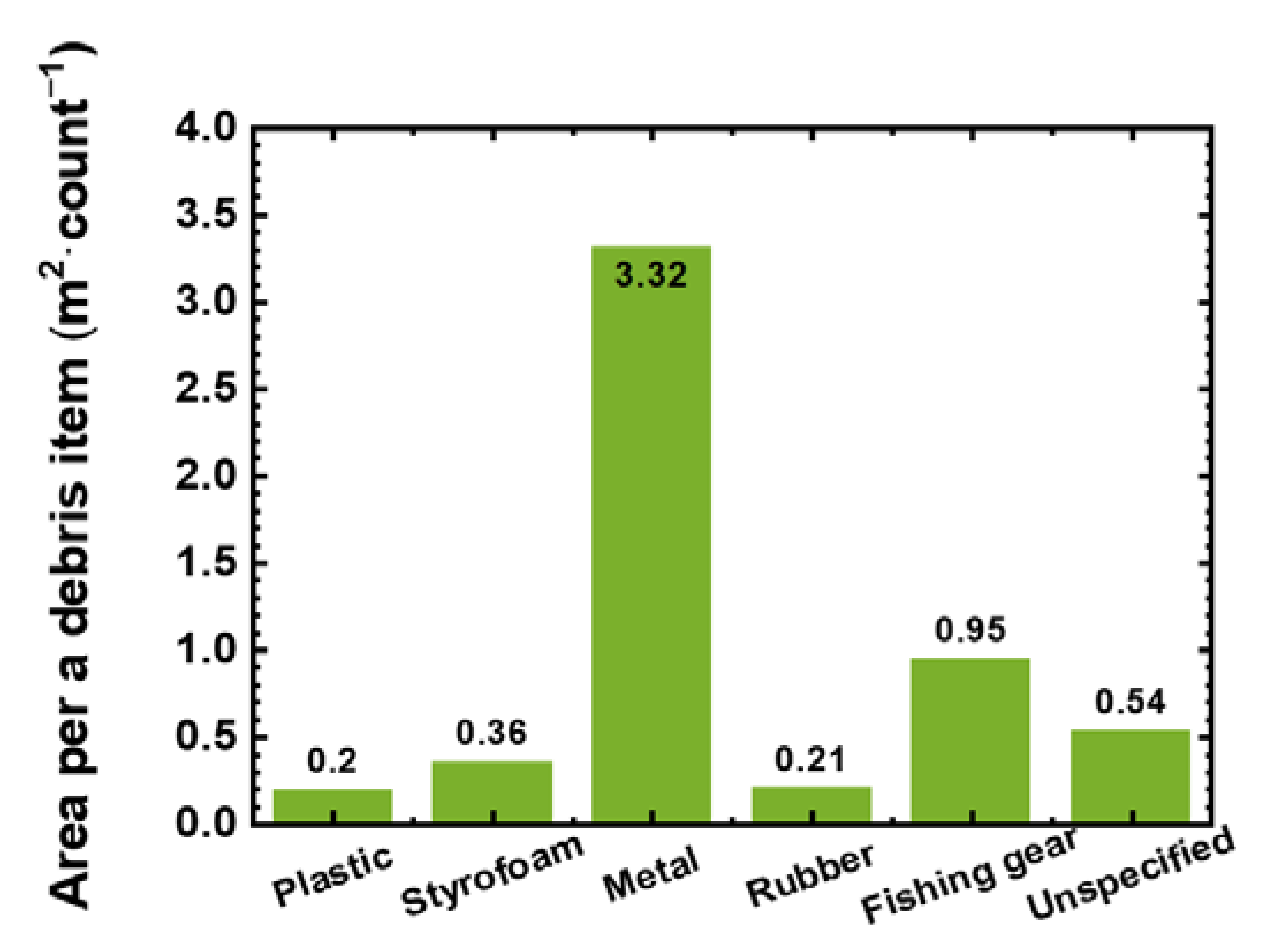
3.2. Covered Area of Debris Items with Class
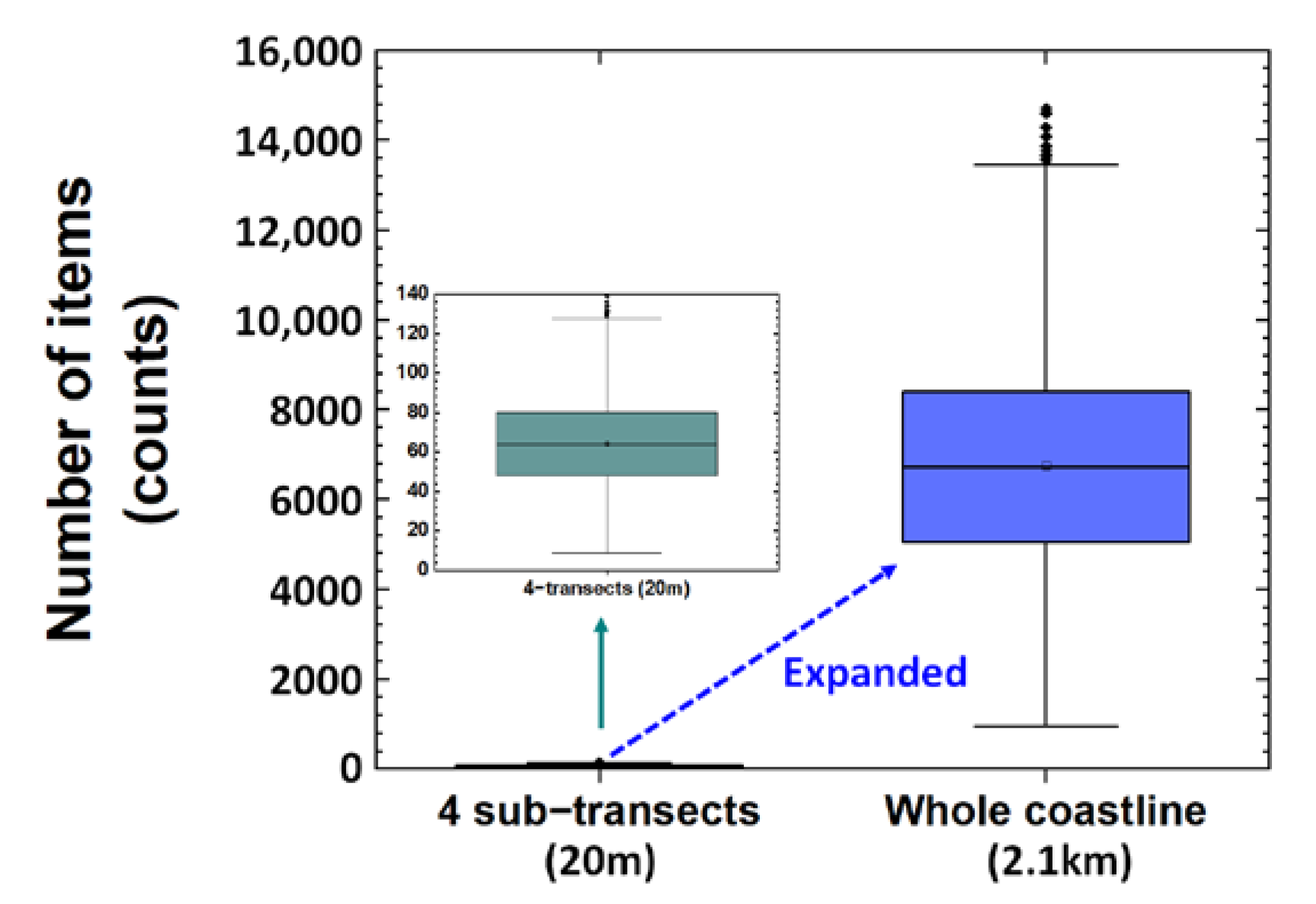
3.3. Comparison of Mapping Method Using UAV and Conventional Monitoring Method
4. Discussion
4.1. Comparison of Mapping Method Using UAV and Conventional Monitoring Method
4.2. Pollution Assessment
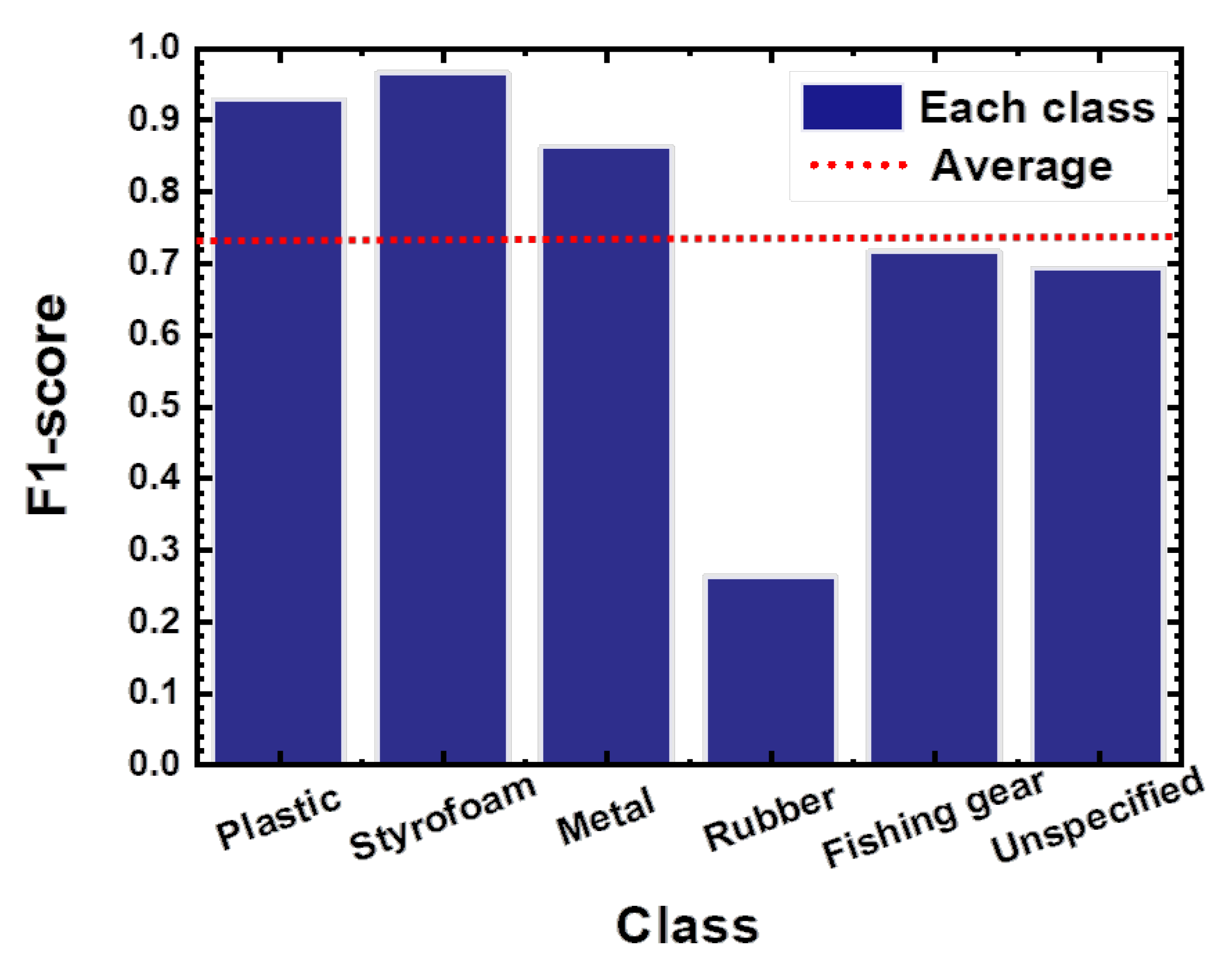
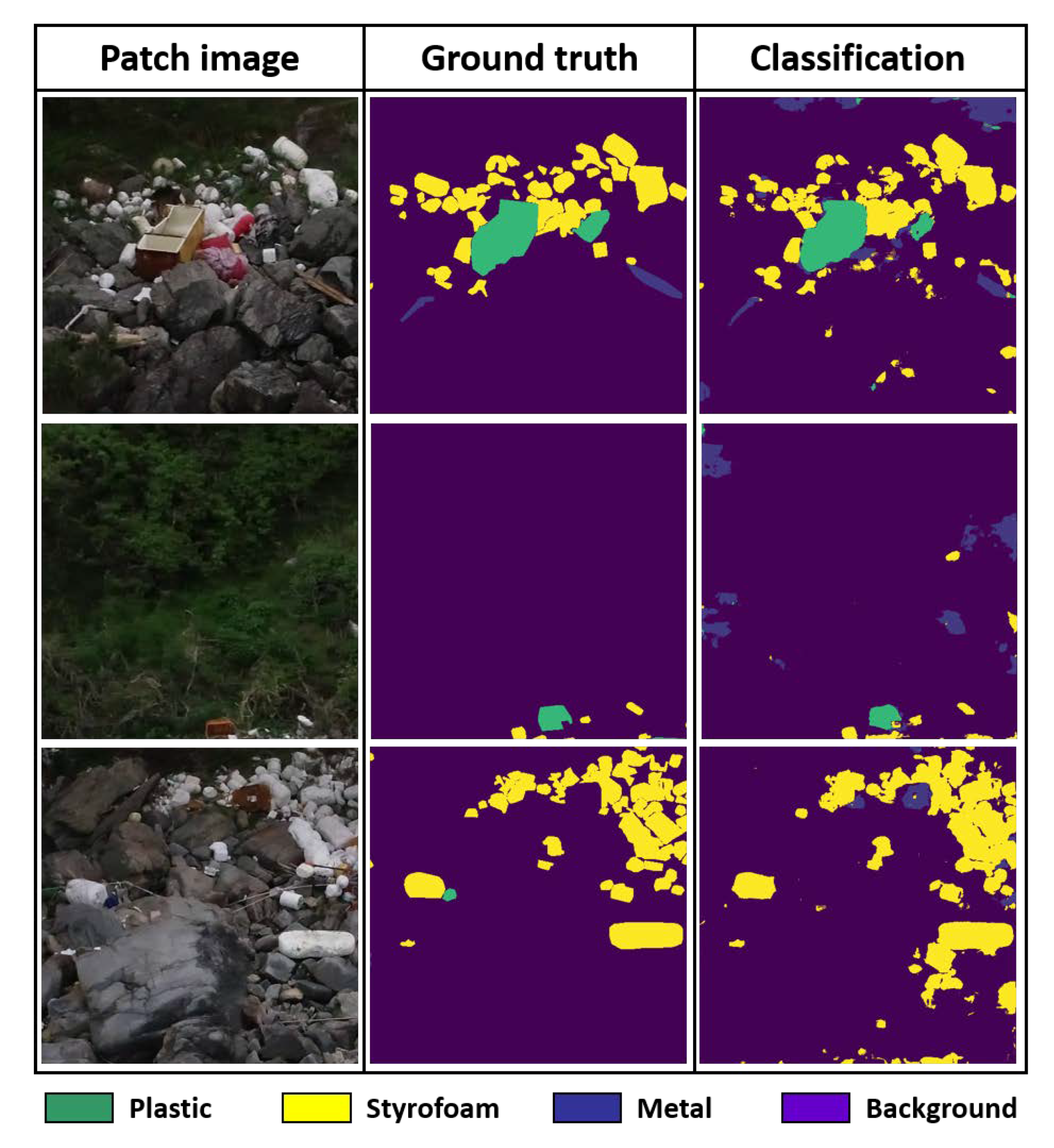
4.3. Accuracy
5. Conclusions
Author Contributions
Funding
Institutional Review Board Statement
Informed Consent Statement
Data Availability Statement
Acknowledgments
Conflicts of Interest
References
- Coe, J.M.; Rogers, D. Marine Debris: Sources, Impacts, and Solutions; Springer: New York, NY, USA, 1996; p. 432. [Google Scholar]
- Galgani, F.; Hanke, G.; Werner, S.; De Vrees, L. Marine Litter within the European Marine Strategy Framework Directive. ICES J. Mar. Sci. 2013, 70, 1055–1064. [Google Scholar] [CrossRef]
- Abalansa, S.; El Mahrad, B.; Vondolia, G.K.; Icely, J.; Newton, A. The Marine Plastic Litter Issue: A Social-Economic Analysis. Sustainability 2020, 12, 8677. [Google Scholar] [CrossRef]
- Mazhandu, Z.S.; Muzenda, E.; Mamvura, T.A.; Belaid, M.; Nhubu, T. Integrated and Consolidated Review of Plastic Waste Management and Bio-Based Biodegradable Plastics: Challenges and Opportunities. Sustainability 2020, 12, 8360. [Google Scholar] [CrossRef]
- Ryan, P.G.; Moore, C.J.; Van Franeker, J.A.; Moloney, C.L. Monitoring the Abundance of Plastic Debris in the Marine Environment. Philos. Trans. R. Soc. B Biol. Sci. 2009, 364, 1999–2012. [Google Scholar] [CrossRef] [PubMed] [Green Version]
- Gall, S.C.; Thompson, R.C. The Impact of Debris on Marine Life. Mar. Pollut. Bull. 2015, 92, 170–179. [Google Scholar] [CrossRef]
- Jambeck, J.R.; Ji, Q.; Zhang, Y.-G.; Liu, D.; Grossnickle, D.M.; Luo, Z.-X. Plastic Waste Inputs from Land into the Ocean. Science 2015, 347, 764–768. [Google Scholar] [CrossRef]
- Löhr, A.; Savelli, H.; Beunen, R.; Kalz, M.; Ragas, A.; Van Belleghem, F. Solutions for Global Marine Litter Pollution. Curr. Opin. Environ. Sustain. 2017, 28, 90–99. [Google Scholar] [CrossRef] [Green Version]
- Guterres, A. The Sustainable Development Goals Report; United Nations: New York, NY, USA, 2021; Available online: https://unsats.un.org/sdgs/report/2021/The-Sustainable-Development-Goals-Report-2021.pdf/ (accessed on 4 July 2021).
- Ali, R.; Shams, Z.I. Quantities and Composition of Shore Debris along Clifton Beach, Karachi, Pakistan. J. Coast. Conserv. 2015, 19, 527–535. [Google Scholar] [CrossRef]
- Asensio-Montesinos, F.; Anfuso, G.; Williams, A.T. Beach Litter Distribution along the Western Mediterranean Coast of Spain. Mar. Pollut. Bull. 2019, 141, 119–126. [Google Scholar] [CrossRef]
- Pervez, R.; Wang, Y.; Ali, I.; Ali, J.; Ahmed, S. The Analysis of the Accumulation of Solid Waste Debris in the Summer Season along the Shilaoren Beach Qingdao, China. Reg. Stud. Mar. Sci. 2020, 34, 101041. [Google Scholar] [CrossRef]
- Pervez, R.; Wang, Y.; Mahmood, Q.; Zahir, M.; Jattak, Z. Abundance, Type, and Origin of Litter on No. 1 Bathing Beach of Qingdao, China. J. Coast. Conserv. 2020, 24, 34. [Google Scholar] [CrossRef]
- Purba, N.P.; Apriliani, I.M.; Dewanti, L.P.; Herawati, H.; Faizal, I. Distribution of Macro Debris at Pangandaran Beach, Indonesia. Int. Sci. J. 2018, 103, 144–156. [Google Scholar]
- Santos, I.R.; Friedrich, A.C.; Ivar do Sul, J.A. Marine Debris Contamination along Undeveloped Tropical Beaches from Northeast Brazil. Environ. Monit. Assess. 2009, 148, 455–462. [Google Scholar] [CrossRef] [PubMed]
- Sarafraz, J.; Rajabizadeh, M.; Kamrani, E. The Preliminary Assessment of Abundance and Composition of Marine Beach Debris in the Northern Persian Gulf, Bandar Abbas City, Iran. J. Mar. Biol. Assoc. UK 2016, 96, 131–135. [Google Scholar] [CrossRef] [Green Version]
- Van Cauwenberghe, L.; Claessens, M.; Vandegehuchte, M.B.; Mees, J.; Janssen, C.R.; Cauwenberghe, V.L.; Claessens, M.; Vandegehuchte, M.B.; Mees, J.; Janssen, C.R. Assessment of Marine Debris on the Belgian Continental Shelf. Mar. Pollut. Bull. 2013, 73, 161–169. [Google Scholar] [CrossRef]
- Hardesty, B.D.; Lawson, T.J.; van der Velde, T.; Lansdell, M.; Wilcox, C. Estimating Quantities and Sources of Marine Debris at a Continental Scale. Front. Ecol. Environ. 2017, 15, 18–25. [Google Scholar] [CrossRef]
- Jang, Y.C.; Ranatunga, R.R.M.K.P.; Mok, J.Y.; Kim, K.S.; Hong, S.Y.; Choi, Y.R.; Gunasekara, A.J.M. Composition and Abundance of Marine Debris Stranded on the Beaches of Sri Lanka: Results from the First Island-Wide Survey. Mar. Pollut. Bull. 2018, 128, 126–131. [Google Scholar] [CrossRef]
- Kumar, A.A.; Sivakumar, R.; Reddy, Y.S.R.; Bhagya Raja, M.V.; Nishanth, T.; Revanth, V. Preliminary Study on Marine Debris Pollution along Marina Beach, Chennai, India. Reg. Stud. Mar. Sci. 2016, 5, 35–40. [Google Scholar] [CrossRef]
- Kusui, T.; Noda, M. International Survey on the Distribution of Stranded and Buried Litter on Beaches along the Sea of Japan. Mar. Pollut. Bull. 2003, 47, 175–179. [Google Scholar] [CrossRef]
- Martin, J.M.; Jambeck, J.R.; Ondich, B.L.; Norton, T.M. Comparing Quantity of Marine Debris to Loggerhead Sea Turtle (Caretta Caretta) Nesting and Non-Nesting Emergence Activity on Jekyll Island, Georgia, USA. Mar. Pollut. Bull. 2019, 139, 1–5. [Google Scholar] [CrossRef]
- McDermid, J.K.; McMullen, L.T. Quantitative Analysis of Small-Plastic Debris on Beaches in the Hawaiian Archipelago. Mar. Pollut. Bull. 2004, 48, 790–794. [Google Scholar] [CrossRef]
- Moore, S.L.; Gregorio, D.; Carreon, M.; Weisberg, S.B.; Leecaster, M.K. Composition and Distribution of Beach Debris in Orange County, California. Mar. Pollut. Bull. 2001, 42, 241–245. [Google Scholar] [CrossRef]
- Nakashima, E.; Isobe, A.; Kako, S.; Itai, T.; Takahashi, S. Quantification of Toxic Metals Derived from Macroplastic Litter on Ookushi Beach, Japan. Environ. Sci. Technol. 2012, 46, 10099–10105. [Google Scholar] [CrossRef] [PubMed]
- APEC (Asia-Pacific Economic Cooperation). Capacity Building for Marine Debris Prevention and Management in the APEC Region; Korea Marine Environment Management Corporation (KOEM) for APEC Secretariat: Yeosu, Korea, 2017; Available online: https://www.apec.org/Publications/2017/12/Capacity-Building-for-Marine-Debris-Prevention-and-Management-in-the-APEC-Region/ (accessed on 4 July 2021).
- Cheshire, A.C.; Adler, E.; Barbiere, J.; Cohen, Y.; Evans, S.; Jarayabhand, S.; Jeftic, L.; Jung, R.T.; Kinsey, S.; Kusui, E.T.; et al. UNEP/IOC Guidelines on Survey and Monitoring of Marine Litter; UNEP Regional Seas Reports and Studies no. 186, IOC Technical Series no. 83. 2009. Available online: https://wedocs.unep.org/bitstream/handle/20.500.11822/13604/rsrs186.pdf? sequence=1&isAllowed=y/ (accessed on 4 July 2022).
- GESAMP (The Joint Group of Experts on the Scientific Aspects of Marine Environmental Protection). Guidelines for the Monitoring and Assessment of Plastic Litter in the Ocean. Rep. Stud. GESAMP 2019, 99, 130. [Google Scholar]
- Lippiatt, S.; Opfer, S.; Arthur, C. Marine Debris Monitoring and Assessment: Recommendations for Monitoring Debris Trends in the Marine Environment; NOAA Technial Memorandun: Silver Spring, MD, USA, 2013. Available online: https://marinedebris.noaa.gov/marine-debris-monitoring-and-assessment-recommendations-monitoring-debris-trends-marine-environment/ (accessed on 4 July 2021).
- MOF (Korea Ministry of Oceans and Fisheries); KOEM (Korea Marine Environment Management Corporation). Korea National Beach Litter Monitoring Program (Phase II); MOF; KOEM: Seoul, Korea, 2017. (In Korean) [Google Scholar]
- Seo, D.-C.; Kim, J.-P. Comparison and Analysis of Monitoring Methods for Marine Debris on Beach. J. Korea Soc. Waste Manag. 2019, 36, 802–810. [Google Scholar] [CrossRef]
- Chang, M.; Xing, Y.Y.; Zhang, Q.Y.; Han, S.J.; Kim, M. A CNN Image Classification Analysis for “clean-Coast Detector” as Tourism Service Distribution. J. Distrib. Sci. 2020, 18, 15–26. [Google Scholar] [CrossRef]
- Fallati, L.; Polidori, A.; Salvatore, C.; Saponari, L.; Savini, A.; Galli, P. Anthropogenic Marine Debris Assessment with Unmanned Aerial Vehicle Imagery and Deep Learning: A Case Study along the Beaches of the Republic of Maldives. Sci. Total Environ. 2019, 693, 133581. [Google Scholar] [CrossRef]
- Fulton, M.; Hong, J.; Islam, M.J.; Sattar, J. Robotic Detection of Marine Litter Using Deep Visual Detection Models. In Proceedings of the 2019 International Conference on Robotics and Automation (ICRA), Montreal, QC, Canada, 20–24 May 2019; pp. 5752–5758. [Google Scholar] [CrossRef] [Green Version]
- Garcia-Garin, O.; Borrell, A.; Aguilar, A.; Cardona, L.; Vighi, M. Floating Marine Macro-Litter in the North Western Mediterranean Sea: Results from a Combined Monitoring Approach. Mar. Pollut. Bull. 2020, 159, 111467. [Google Scholar] [CrossRef]
- Gonçalves, G.; Andriolo, U.; Pinto, L.; Bessa, F. Mapping Marine Litter Using UAS on a Beach-Dune System: A Multidisciplinary Approach. Sci. Total Environ. 2020, 706, 135742. [Google Scholar] [CrossRef]
- Kako, S.; Morita, S.; Taneda, T. Estimation of Plastic Marine Debris Volumes on Beaches Using Unmanned Aerial Vehicles and Image Processing Based on Deep Learning. Mar. Pollut. Bull. 2020, 155, 111127. [Google Scholar] [CrossRef]
- Martin, C.; Parkes, S.; Zhang, Q.; Zhang, X.; McCabe, M.F.; Duarte, C.M. Use of Unmanned Aerial Vehicles for Efficient Beach Litter Monitoring. Mar. Pollut. Bull. 2018, 131, 662–673. [Google Scholar] [CrossRef] [PubMed] [Green Version]
- Moy, K.; Neilson, B.; Chung, A.; Meadows, A.; Castrence, M.; Ambagis, S.; Davidson, K. Mapping Coastal Marine Debris Using Aerial Imagery and Spatial Analysis. Mar. Pollut. Bull. 2018, 132, 52–59. [Google Scholar] [CrossRef] [PubMed]
- Papakonstantinou, A.; Batsaris, M.; Spondylidis, S.; Topouzelis, K. A Citizen Science Unmanned Aerial System Data Acquisition Protocol and Deep Learning Techniques for the Automatic Detection and Mapping of Marine Litter Concentrations in the Coastal Zone. Drones 2021, 5, 6. [Google Scholar] [CrossRef]
- Jakovljevic, G.; Govedarica, M.; Alvarez-Taboada, F. A Deep Learning Model for Automatic Plastic Mapping Using Unmanned Aerial Vehicle (UAV) Data. Remote Sens. 2020, 12, 1515. [Google Scholar] [CrossRef]
- Bao, Z.; Sha, J.; Li, X.; Hanchiso, T.; Shifaw, E. Monitoring of Beach Litter by Automatic Interpretation of Unmanned Aerial Vehicle Images Using the Segmentation Threshold Method. Mar. Pollut. Bull. 2018, 137, 388–398. [Google Scholar] [CrossRef]
- Kataoka, T.; Murray, C.C.; Isobe, A. Quantification of Marine Macro-Debris Abundance around Vancouver Island, Canada, Based on Archived Aerial Photographs Processed by Projective Transformation. Mar. Pollut. Bull. 2018, 132, 44–51. [Google Scholar] [CrossRef] [PubMed]
- Song, K.; Jung, J.; Hyun, S.; Park, S. A Comparative Study of Deep Learning-Based Network Model and Conventional Method to Assess Beach Debris Standing-Stock. Mar. Pollut. Bull. 2021, 168, 112466. [Google Scholar] [CrossRef]
- Ronneberger, O.; Fischer, P.; Thomas, B. UNet: Convolutional Networks for Biomedical Image Segmentation. IEEE Access 2015, 9, 16591–16603. [Google Scholar] [CrossRef]
- Bekkar, M.; Djemaa, H.K.; Alitouche, T.A. Evaluation Measures for Models Assessment over Imbalanced Data Sets. J. Inf. Eng. Appl. 2013, 3, 27–38. [Google Scholar]
- Cui, Y.; Jia, M.; Lin, T.Y.; Song, Y.; Belongie, S. Class-Balanced Loss Based on Effective Number of Samples. In Proceedings of the IEEE Computer Society Conference on Computer Vision and Pattern Recognition, Long Beach, CA, USA, 15–20 June 2019; pp. 9260–9269. [Google Scholar] [CrossRef] [Green Version]
- Shorten, C.; Khoshgoftaar, T.M. A Survey on Image Data Augmentation for Deep Learning. J. Big Data 2019, 6, 60. [Google Scholar] [CrossRef]
- Sheavly, S.B. National Marine Debris Monitoring Program—Lessons Learned. Report Prepared for the United States Environmental Protection Agency. 2010. Available online: http://www.portalasporta.it/dati_plastica/Marine_Debris_2010.pdf/ (accessed on 4 July 2022).
- Ghaffari, S.; Bakhtiari, A.R.; Ghasempouri, S.M.; Nasrolahi, A. The Influence of Human Activity and Morphological Characteristics of Beaches on Plastic Debris Distribution along the Caspian Sea as a Closed Water Body. Environ. Sci. Pollut. Res. 2019, 26, 25712–25724. [Google Scholar] [CrossRef] [PubMed]
- Banerjee, B.P.; Sharma, V.; Spangenberg, G.; Kant, S. Machine Learning Regression Analysis for Estimation of Crop Emergence Using Multispectral UAV Imagery. Remote Sens. 2021, 13, 2918. [Google Scholar] [CrossRef]
- Yang, Y.; Lin, Z.; Liu, F. Stable Imaging and Accuracy Issues of Low-Altitude Unmanned Aerial Vehicle Photogrammetry Systems. Remote Sens. 2016, 8, 316. [Google Scholar] [CrossRef] [Green Version]


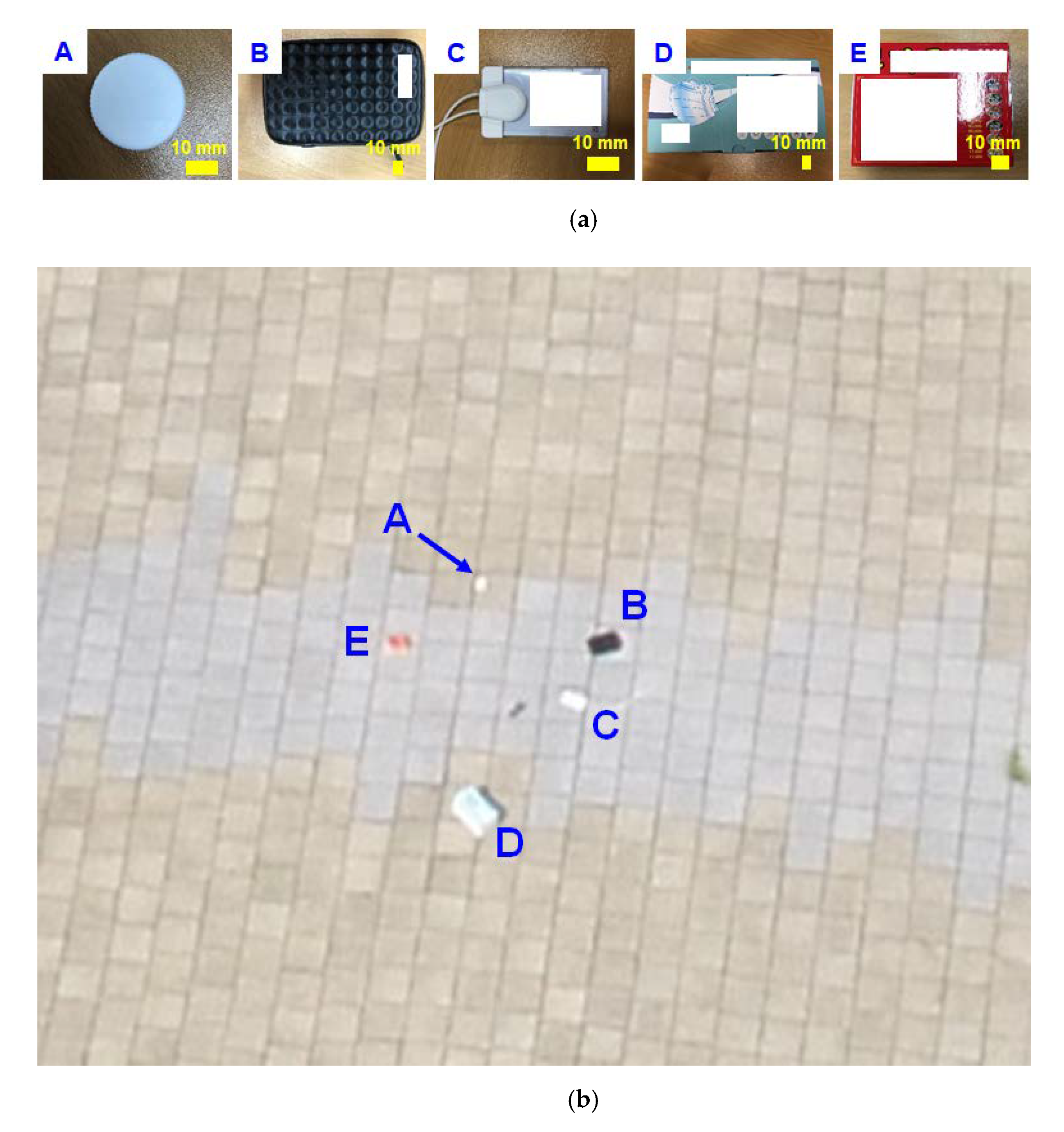
| Sample | Actual Area (m2) | Number of Pixels (Counts) | Area per Unit Pixel (m2) |
|---|---|---|---|
| A | 0.71 × 10⁻³ | 25 | 2.84 × 10⁻⁵ |
| B | 13.75 × 10⁻³ | 56 | 2.45 × 10⁻⁵ |
| C | 5.55 × 10⁻³ | 48 | 1.16 × 10⁻⁵ |
| D | 20.47 × 10⁻³ | 95 | 2.15 × 10⁻⁵ |
| E | 7.60 × 10⁻³ | 176 | 4.32 × 10⁻⁵ |
| Mean (standard deviation) | 2.58 × 10⁻⁵ (0.79 × 10⁻⁵) |
| Categories | Pixels of Labeled Items | Class Weight |
|---|---|---|
| Plastic | 3,247,265 | 15.06 |
| Styrofoam | 4,911,259 | 9.93 |
| Metal | 303,451 | 160.68 |
| Rubber | 25,431 | 1917.29 |
| Fishing gear | 425,719 | 114.53 |
| Unspecified | 918,175 | 53.10 |
Publisher’s Note: MDPI stays neutral with regard to jurisdictional claims in published maps and institutional affiliations. |
© 2022 by the authors. Licensee MDPI, Basel, Switzerland. This article is an open access article distributed under the terms and conditions of the Creative Commons Attribution (CC BY) license (https://creativecommons.org/licenses/by/4.0/).
Share and Cite
Song, K.; Jung, J.-Y.; Lee, S.H.; Park, S.; Yang, Y. Assessment of Marine Debris on Hard-to-Reach Places Using Unmanned Aerial Vehicles and Segmentation Models Based on a Deep Learning Approach. Sustainability 2022, 14, 8311. https://doi.org/10.3390/su14148311
Song K, Jung J-Y, Lee SH, Park S, Yang Y. Assessment of Marine Debris on Hard-to-Reach Places Using Unmanned Aerial Vehicles and Segmentation Models Based on a Deep Learning Approach. Sustainability. 2022; 14(14):8311. https://doi.org/10.3390/su14148311
Chicago/Turabian StyleSong, Kyounghwan, Jung-Yeul Jung, Seung Hyun Lee, Sanghyun Park, and Yunjung Yang. 2022. "Assessment of Marine Debris on Hard-to-Reach Places Using Unmanned Aerial Vehicles and Segmentation Models Based on a Deep Learning Approach" Sustainability 14, no. 14: 8311. https://doi.org/10.3390/su14148311
APA StyleSong, K., Jung, J.-Y., Lee, S. H., Park, S., & Yang, Y. (2022). Assessment of Marine Debris on Hard-to-Reach Places Using Unmanned Aerial Vehicles and Segmentation Models Based on a Deep Learning Approach. Sustainability, 14(14), 8311. https://doi.org/10.3390/su14148311