TRNSYS Simulation and Experimental Validation of Internal Temperature and Heating Demand in a Glass Greenhouse

Abstract

The energy demand in greenhouses is enormous, and high-performance covering materials and thermal screens with varying radiometric properties are used to optimise the energy demand in building energy simulations (BES). Transient System Simulation (TRNSYS) software is a common BES tool used to model the thermal performance of buildings. The calculation of the greenhouse internal temperature and heating demand in TRNSYS involves the solution of the transient heat transfer processes. This study modelled the temperature and heating demand of two multi-span glass greenhouses with concave (farm A) and convex (farm B) shapes. This study aims to investigate the influence of the different BES longwave radiation modes on greenhouse internal temperature in different zones and the heating demand of a conditioned zone. The standard hourly simulation results were compared with the experimental data. The results showed that the standard and detailed modes accurately predicted greenhouse internal temperature (the Nash–Sutcliffe efficiency coefficient (NSE) > 0.7 for all three zones separated by thermal screens) and heating demand (NSE > 0.8) for farms A and B. The monthly heating demand predicted by the simple and standard radiation modes for farm A matched the experimental measurements with deviations within 27.7% and 7.6%, respectively. The monthly heating demand predicted by the simple, standard, and detailed radiation modes for farm B were similar to the experimental measurements with deviations within 10.5%, 6.7%, and 2.9%, respectively. In the order of decreasing accuracy, the results showed that the preferred radiation modes for the heating demand were standard and simple for farm A, and detailed, standard, and simple for farm B.

1. Introduction

Greenhouse farming aims to grow warm-season crops in winter and has been utilised to solve food shortages year-round. The control of indoor air, especially under adverse weather conditions, is crucial for crop production in greenhouses [1,2,3]. The energy consumption for the indoor air control contributes to 50% of the total cost of greenhouse production in many countries [4], making the greenhouse sector one of the most energy-intensive agricultural sectors, with significant economic and environmental impacts [5,6].

Passive energy-saving strategies reduce greenhouse energy consumption. This involves selecting high-performance greenhouse-covering materials and thermal screens to limit the amount of solar radiation the crop receives in summer and the rate of heat loss in winter [7]. Using thermal screens reduces the heat loss rate by 23–24% [8], and they are placed either internally or externally to ensure a favourable microclimate for the crop [9]. Most growers prefer internal thermal screens use owing to the increased heat retention [10] and reduced surface-to-volume ratio of the heating zone, leading to a reduction in the heating cost [11].

Several studies have used numerical modelling to assess the impact of different covering materials and thermal screens on greenhouse microclimate and energy consumption [12,13,14]. Zhang et al. [15] solved unsteady state equations using MATLAB to study the thermal performance of a greenhouse by altering the cover transmittance and absorbance for beam, diffuse, and ground-reflected radiations in a glass greenhouse. The surface radiative properties change with time and impact energy demand. Another study [16] investigated the effect of different plastic materials with spectral radiative properties ranging from 0.2 to 28 μm. The annual heating demand of the greenhouse was reduced by 6.3% using appropriate greenhouse materials in the developed model.

EnergyPlus and TRNSYS are building energy simulation (BES) tools for modelling the thermal performance of different types of buildings [17]. Within the simulation environment of these tools, there exist pre-existing components to construct a model [18]. The users have the flexibility of varying different parameters on each component to suit the application the model is intended for. The major setback of these tools for greenhouse modelling is their inability to account for the influence of crop and their environmental control systems [19,20]. Unlike EnergyPlus, TRNSYS permits users to develop new components and link with other simulation tools [7]. This makes TRNSYS, which was primarily developed for residential and commercial buildings, able to be continuously improved for greenhouse modelling. The Gembloux Dynamic Greenhouse Climate Model based on heat and mass balance of greenhouse layers was linked with TRNSYS as a sub-model for greenhouse air renewal rate and canopy resistance in a naturally ventilated greenhouse [21]. The model accurately predicted the greenhouse microclimate parameters, but there was an overestimation of the ventilation rate, mostly during night time. Ahamed et al. [22] also developed a TRNSYS model to predict the heating demand in a Chinese-style solar greenhouse (CSG). The results were compared with a heating simulation model (CSGHEAT) from MATLAB. The heating load from TRNSYS resulted in significant errors from assumptions such as constant infiltration rate, fixed scheduled for thermal screens and moisture gain.

A solar-radiation-based control for thermal screens as operated in the CSGHEAT model was implemented in TRNSYS using the equation editor in the simulation studio [23]. Based on the control, the multi-layer thermal screens reduced greenhouse energy consumption compared with double and single thermal screens investigated. The thermal screens also ensured a temperature difference of approximately 5 °C between the three zones in the multi-span greenhouse. However, with a unidirectional heat transfer model, there was no significant temperature difference within four zones of the greenhouse with moveable thermal screens on the north and south walls [24]. Asa’d et al. [25] performed a parametric analysis using TRNSYS to study the effect of the cooling and heating setpoint temperatures, cover materials, rock-bed air flow rate, and mechanical ventilation to improve the overall design of a greenhouse. The study concluded that the U-value of the materials and the rock-bed airflow rate have the most significant effect on the greenhouse internal temperature. Rabiu et al. [26] used TRNSYS and hotbox to evaluate the greenhouse energy-saving screen properties. The investigation also concluded that the screens’ infiltration has the most significant impact on their U-values.

Scope of the Study

BES tools are used to investigate the effect of the different parameters on greenhouse microclimate and predict the most favourable operating conditions that minimise the energy consumption. With TRNSYS, several studies have reported the effect of the regime type, environmental control systems, covering materials, greenhouse shape, and orientation on the thermal performance of the greenhouse, with no consideration to the radiation modes [27,28,29]. The accurate modelling of the solar heat gains in the greenhouse with the different radiation modes in TRNSYS is also an important aspect that should be considered. To this end, a multi-span glass greenhouse area of 3942 m² was divided in two (farm A, 2160 m², and farm B, 1782 m²) based on their geometry to study the effect of the radiation modes on the internal temperature and heating demand of the greenhouse. The resulting TRNSYS simulation results were validated with the experimental measurements of farm A (concave-shaped) and farm B (convex-shaped) greenhouses. The major findings from this research will assist greenhouse growers, researchers, and engineers to choose the best radiation mode to model the thermal performance of a greenhouse depending on the greenhouse shape.

2. Materials and Methods

2.1. Description of the Experimental Site

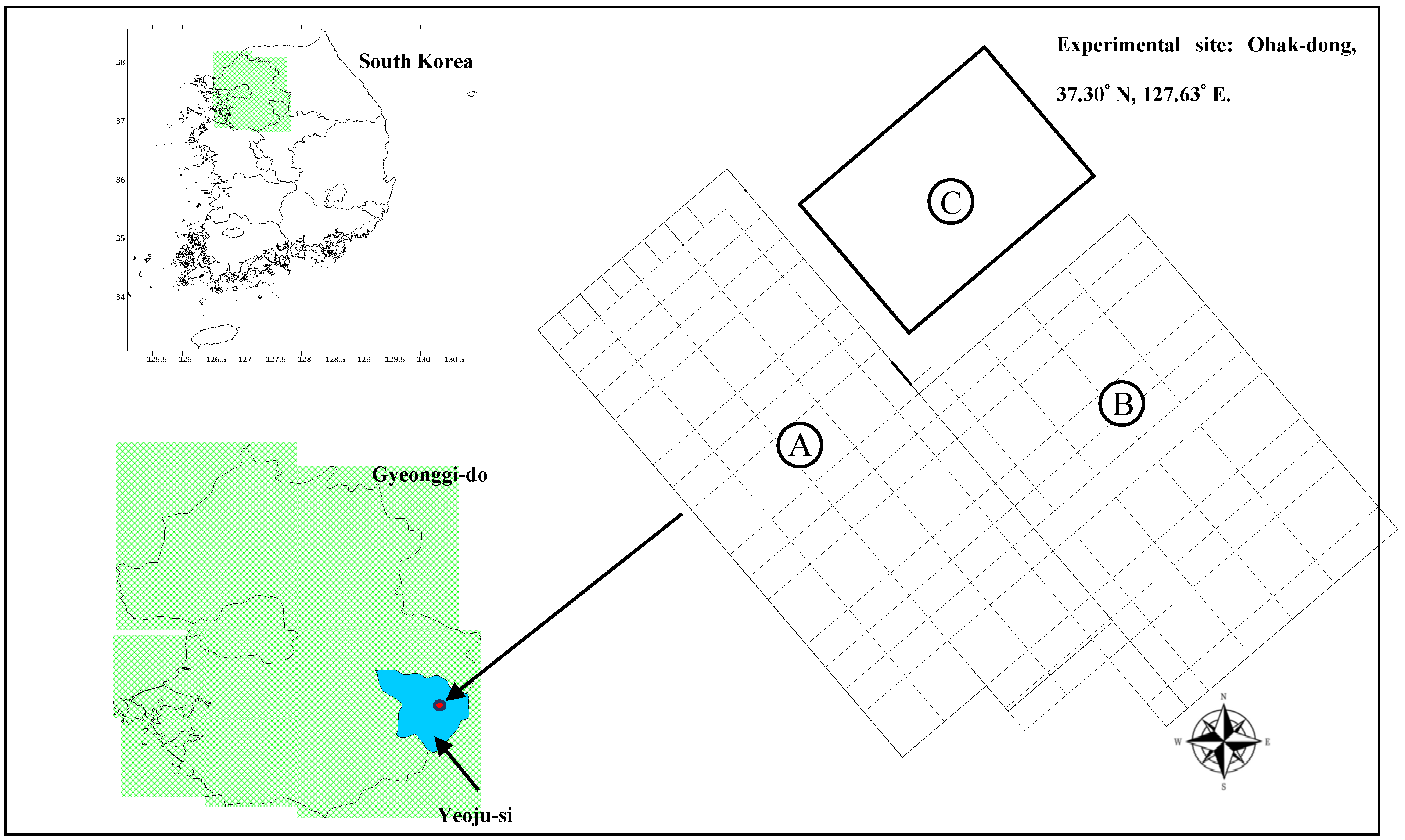
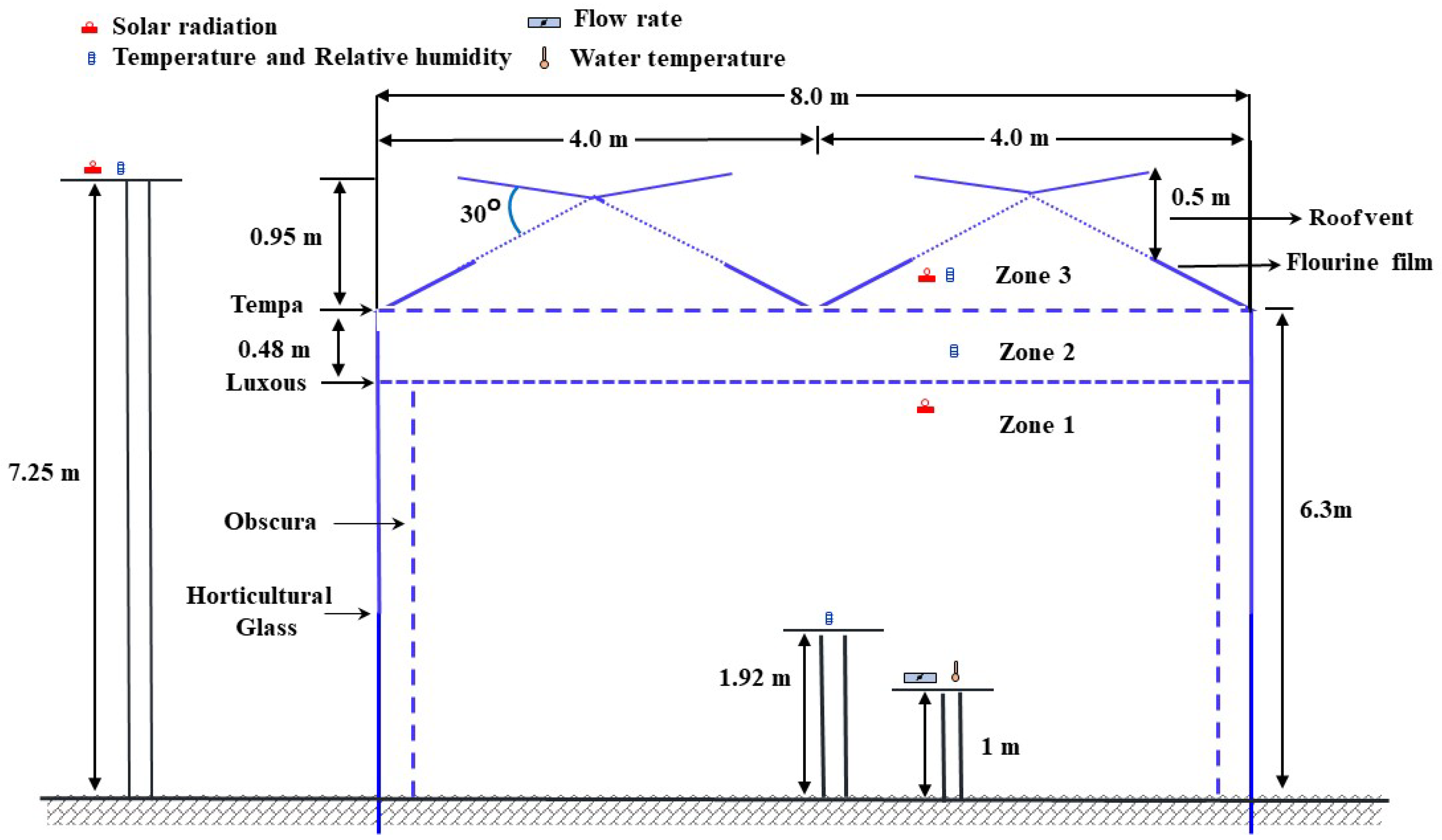
The experimental greenhouse (Purme social farm, Figure 1) is located in Ohak-dong, Yeoju-si, a small town in Gyeonggi-do, western South Korea. The experimental site was in a temperate climate with lengthy, hot, rainy, and partially cloudy summers, while winters are short, cold, snowy, and largely clear [30]. The farm covers a gross area of 4374 m² in three parts, farm A (2160 m²), farm B (1782 m²), and a packaging room (432 m²), represented by A, B, and C, respectively, in Figure 2. Farms A and B are Venlo-roofed, multi-span, glass greenhouses with dimensions of 32 m × 67.5 m × 7.25 m and 36 m × 49.5 m × 7.25 m, respectively. The vertical view of one of the spans and sensor positions are shown in Figure 3. The total net conditioned volume of the greenhouse was 22,942.4 m³, with a net conditioned area of 3942 m².

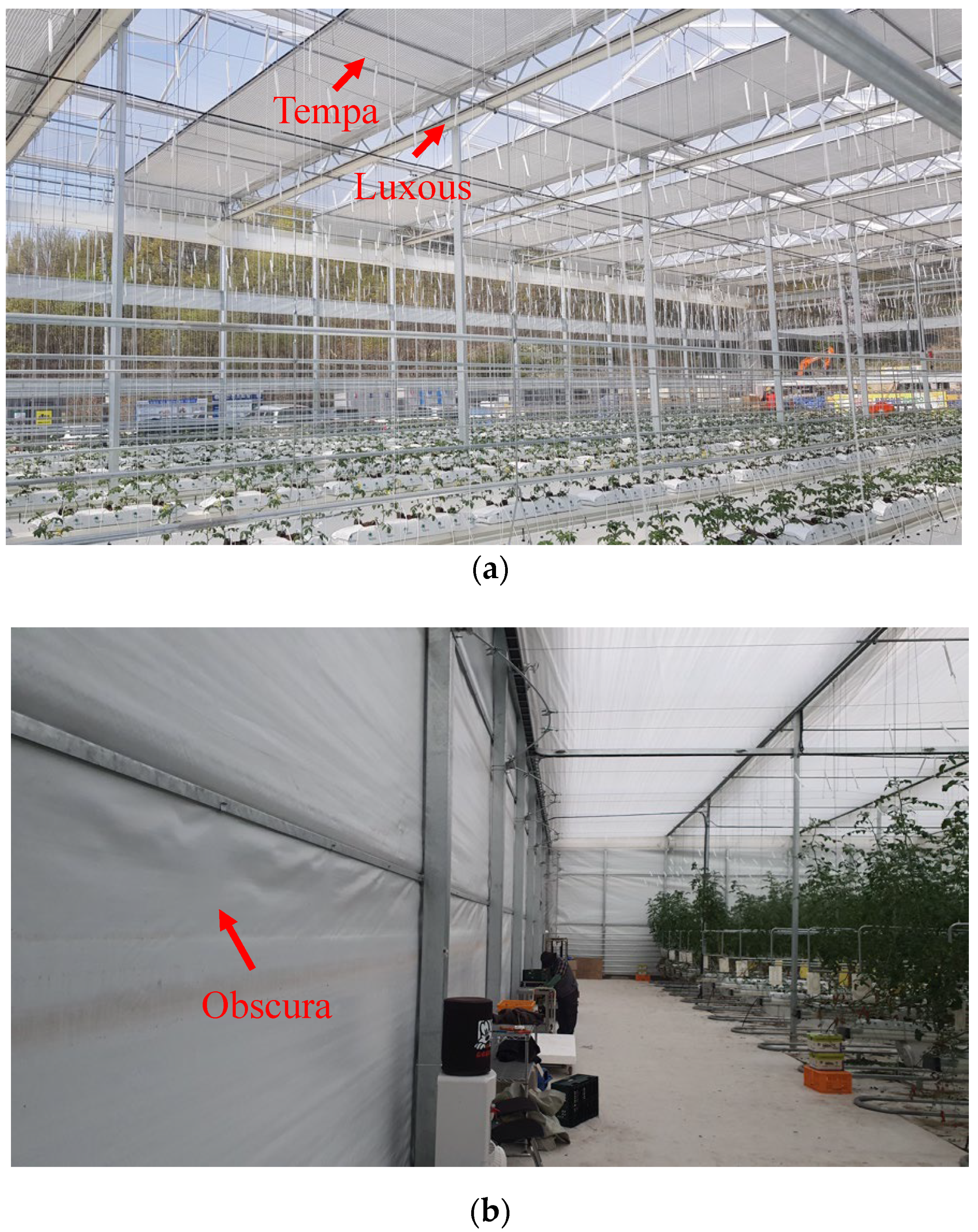
The greenhouse was fitted with passive, eco-friendly materials (transparent and opaque) for internal climate management. The sides and roof of the greenhouse were covered with horticultural glass (HG) and fluorine film. Retractable horizontal (Tempa and Luxous) and vertical (Obscura) thermal screens were installed (Figure 4). The white surface of Obscura helps to reflect light onto the crop to enhance crop growth. Tempa is a shading screen used during the summer to minimise excessive solar radiation during the day. It reflects and diffuses sunlight to moderate the solar heat load and cools the greenhouse. However, because most shading screens are used as thermal screens during winter, Tempa is also deployed at night to enhance heat retention. Luxous is a thermal screen that aids retaining heat at night to maintain a stable greenhouse temperature. The horizontal thermal screens divided the greenhouse into conditioned (zone 1) and unconditioned (zones 2 and 3) zones to reduce the greenhouse heating area. Sensors were fixed in each zone to monitor the effect of the screens on the macro-environment.

Outside weather data were recorded during winter between December 2021 and March 2022. The recorded data included the solar radiation, temperature, and relative humidity. Other required outside weather data for the BES model, such as wind speed, wind direction, and ambient pressure, were downloaded from the Korean Meteorological Administration (KMA), Icheon (Station 203, 37.26° N 127.48° E) [31]. The details of the recorded data are listed in

Table 1. Details of the recorded weather data.

Parameter	Measurement Method	Sensor	Precision of Sensor	Characteristics
Ambient temperature (°C)	9 places at 1.92 m above the ground (zone 1) and 1 place at the centre of zone 2 and 3	HOBO MX1102A	±0.5%	Field recorded
Relative humidity (%)	9 places at 1.92 m above the ground (zone 1) and 1 place at the centre of zone 2 and 3	HOBO MX1102A	±0.5%	Field recorded
Solar radiation (Wm−2)	7.25 m above the ground (outside the greenhouse)	CMP3 pyranometer	±2%	Field recorded
Water temperature (°C)	1 m above the ground (zone 1)	I-Sensor, PT 100	±0.3 °C	Field recorded
Flow rate (LPM)	1 m above the ground (zone 1)	KFCM-1000 K-2101083-2	±5%	Field recorded
Wind speed (ms−1)	10 m above the ground (at the weather station)	Clima sensor, US, Thies Clima	±5%	KMA
Wind direction (degree)	10 m above the ground (at the weather station)	Clima sensor, US, Thies Clima	±5%	KMA
Ambient pressure (hPa)	10 m above the ground (at the weather station)	PTB-220TS, VAISALA	±5 hPa	KMA

. The windspeed data were measured at a height that was different from the eave height of the greenhouse. The data were modified according to the power law in Equation (1):

$$V_h=V_o(\frac{h}{h_o}{)}^{\propto },$$

(1)

where $V_h$ is the calculated wind speed (ms⁻¹) at height h (m) of the greenhouse, $V_o$ is the downloaded KMA station wind speed (ms⁻¹) at height $h_o$ (m), and ∝ is the power law exponent. The power law exponent is an empirically derived coefficient that increases in value with increase in terrain roughness. In an experiment conducted by Jung et al. [32] in a coastal region (Buan-gu) similar to the experimental site, the power law exponent was 0.28.

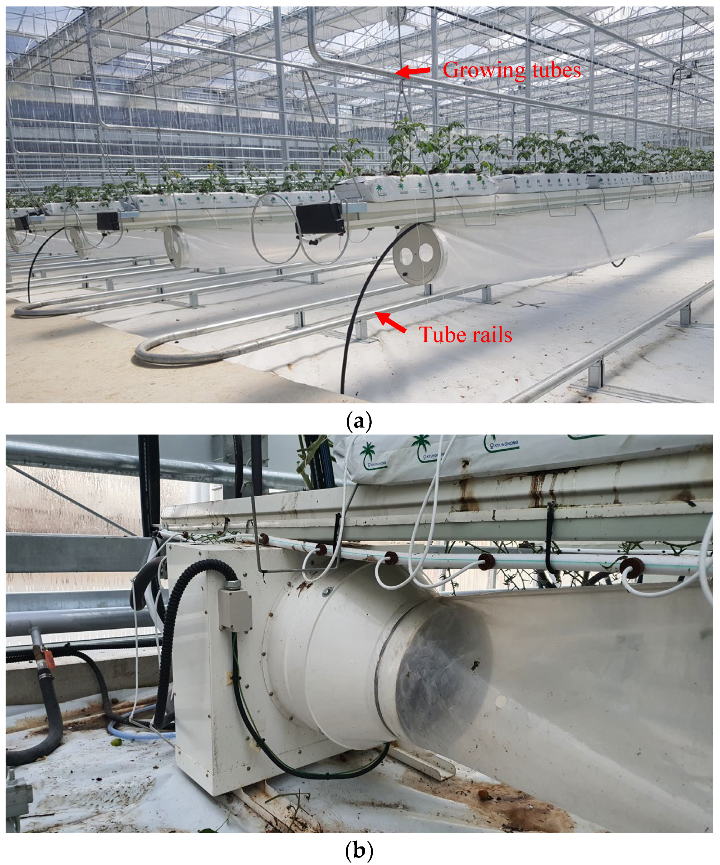
The greenhouse design combines different strategies to supply heating energy via a fan coil unit, growing tubes, and tube rails (Figure 5) to ensure adequate thermal comfort of crops under low ambient temperature conditions. The water temperature and flow rate were monitored to calculate the energy consumed using Equation (2). The locations and specifications of the water temperature and flow rate sensors are detailed in Figure 3 and Table 1, respectively.

$$Q=\dot{m}·C_p·\Delta t,$$

(2)

where Q is the amount of energy consumed (kcalh⁻¹), $\dot{m}$ is the mass flow rate (kgh⁻¹), $C_p$ is the specific heat capacity of water (kcalkg⁻¹$\mathrm{K}$⁻¹), and $\Delta t$ is the difference between inlet and outlet water temperatures ($\mathrm{K}$).

2.2. Greenhouse Material Properties

Some properties of the greenhouse-covering materials have been presented in the literature. Valera et al. [33], Rafiq et al. [34], and Rabiu et al. [26] detailed the properties of HG, Tempa, and Luxous, respectively (

Table 2. Properties of greenhouse covering materials from the literature.

Cover Characteristics	Covering Material	Thermal Screens
	HG	Tempa	Luxous
Thickness (mm)	4	0.31	0.30
Solar transmittance (front)	0.89	0.10	0.58
Solar transmittance (back)	0.89	0.12	0.57
Solar reflectance (front)	0.08	0.65	0.30
Solar reflectance (back)	0.08	0.51	0.25
Visible radiation transmittance (front)	0.91	0.10	0.58
Visible radiation transmittance (back)	0.91	0.12	0.57
Visible radiation reflection (front)	0.08	0.65	0.30
Visible radiation reflection (back)	0.08	0.51	0.25
Thermal radiation transmittance	0.1	0.05	0.38
Thermal radiation emission (front)	0.90	0.20	0.44
Thermal radiation emission (back)	0.90	0.33	0.44
Thermal conductivity (Wm−1K−1)	0.10	0.52	0.06
Infiltration (m3h−1m2)	-	3.62	6.45

). Ground and steel are treated as opaque in TRNBuild (a TRNSYS building interface), with properties listed in

Table 3. Properties of the opaque materials.

Materials	Thickness (m)	Thermal Conductivity (kJh−1m−1K−1)	Thermal Capacity (kJkg−1K−1)	Density (kgm−3)	Convective Heat Transfer Coefficient (kJh−1m−2K−1)
					Front	Back
Ground	0.1000	0.97	0.75	2900	11	0.001
Steel	0.05	54	1.8	7800	11	64

. Fluorine film and Obscura are novel greenhouse materials whose properties were determined experimentally.

The thickness (mm) of the fluorine film and Obscura was measured using an electronic digital calliper (TED PELLA, Inc., Redding, CA, USA), and the thermal conductivity (${\mathrm{Wm}}^{-1}{\mathrm{K}}^{-1}$) was measured using a QTM-500 (Kyoto Electronics MFG. Co., Ltd., Kyoto, Japan) thermal conductivity meter. The infiltration through the materials was measured using a procedure detailed in our previous study [26].

There are two main approaches for determining radiative properties: spectrophotometry and the radiation balance method (RBM) [35]. The suitability of fluorine film and Obscura in the BES model was confirmed using these two methods. The shortwave and longwave properties were determined in the laboratory using a haze meter (Murakami, HM-150) and Fourier transform infrared spectrophotometer. The RBM experimental procedure for longwave and shortwave radiation is shown in Figure 6 and Figure 7. Figure 8 shows the experimental setup for the fluorine film (left) and Obscura (right). The experiments were conducted on the open roof of a building of height 15 m for unobstructed sky radiation.

The longwave radiation is calculated using Equations (3)–(5):

$$Q_b=E_s+\left({\rho }_L·Q_a\right)+\left(Q_d·{\tau }_L\right),$$

(3)

$$Q_c=E_s+\left({\tau }_L·Q_a\right)+\left(Q_d·{\rho }_L\right){,}_{ }$$

(4)

$$Q_d=E_b+\left({\rho }_b+\mu \right)E_s+\left({\rho }_b-\mu \right)\left({\rho }_L·Q_d\right)+\left({\rho }_b-\mu \right)\left({\tau }_L·Q_a\right),$$

(5)

where Q_b is the upward longwave radiation from the material to the sky (Wm⁻²), Q_c is the upward longwave radiation from the material to the black fabric during the night (Wm⁻²), Q_d is the inward longwave radiation from the black fabric toward the material (Wm⁻²), Q_a is the inward sky radiation toward the material (Wm⁻²), ρ_L is the longwave reflectance of the material, τ_L is the longwave transmittance of the material, and E_s is the emissive power of the material (Wm⁻²) from the Stefan–Boltzmann’s law. E_s is calculated using Equation (6):

$$E_s=\sigma T_b{}^4{\epsilon }_b,$$

(6)

where $\sigma$ is the Stefan–Boltzmann constant, $T_b$ and ${\epsilon }_b$ are the surface temperature and emissivity of the black fabric, respectively.

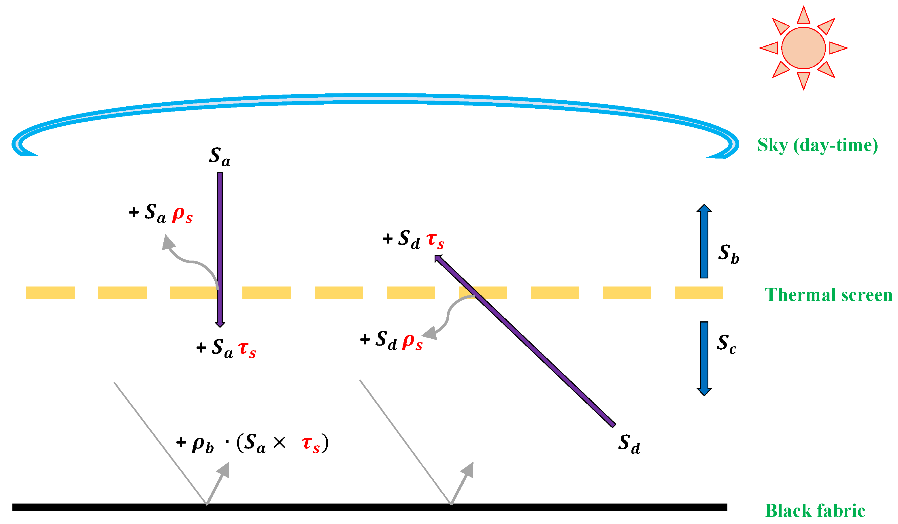
The shortwave radiation is calculated using Equations (7) and (8):

$$S_b=\left({\rho }_s·S_a\right)+({\tau }_s·S_d),$$

(7)

$$S_c=\left({\rho }_{s }·S_d\right)+({\tau }_s·S_a),$$

(8)

where S_b is the outward shortwave radiation from the material toward the sky, S_c is the outward shortwave radiation from the material toward the black material, ρ_s is the reflectance of the material, τ_s is the transmittance of the material, and S_a and S_d are the downward shortwave radiation from the sky and the radiation from the black fabric toward the material, respectively.

2.3. Greenhouse Simulation Modelling in TRNSYS 18

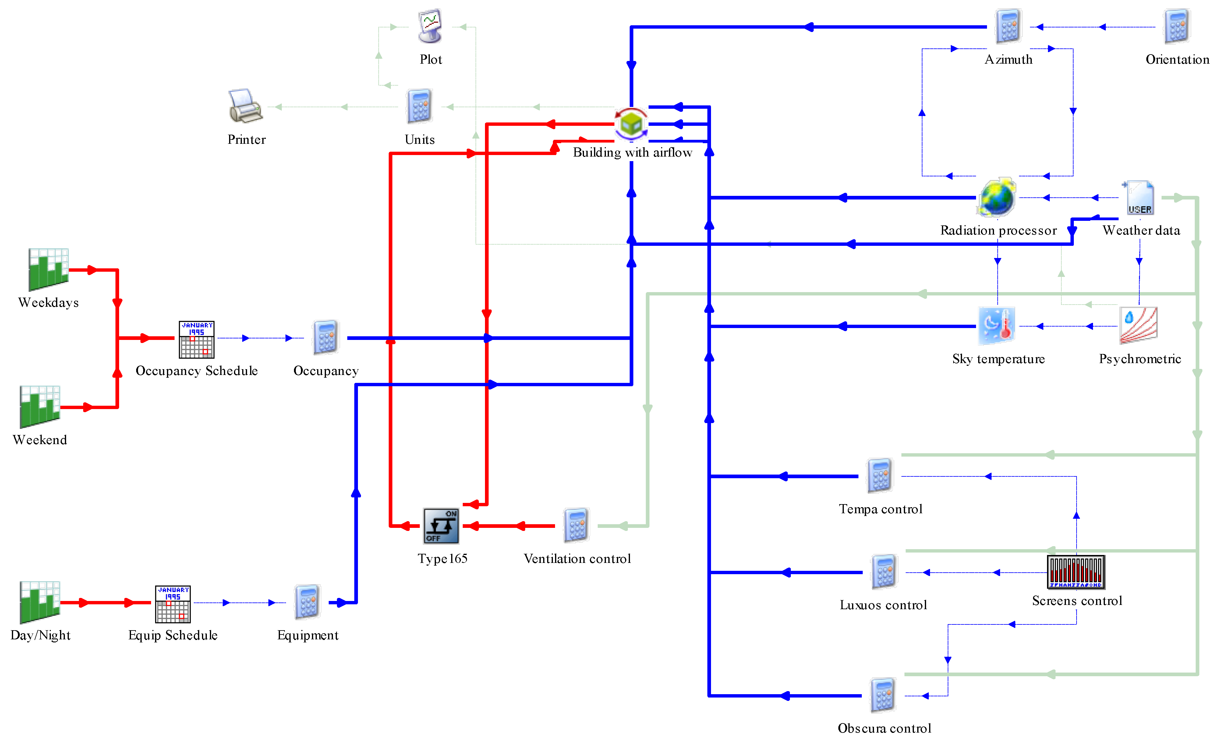
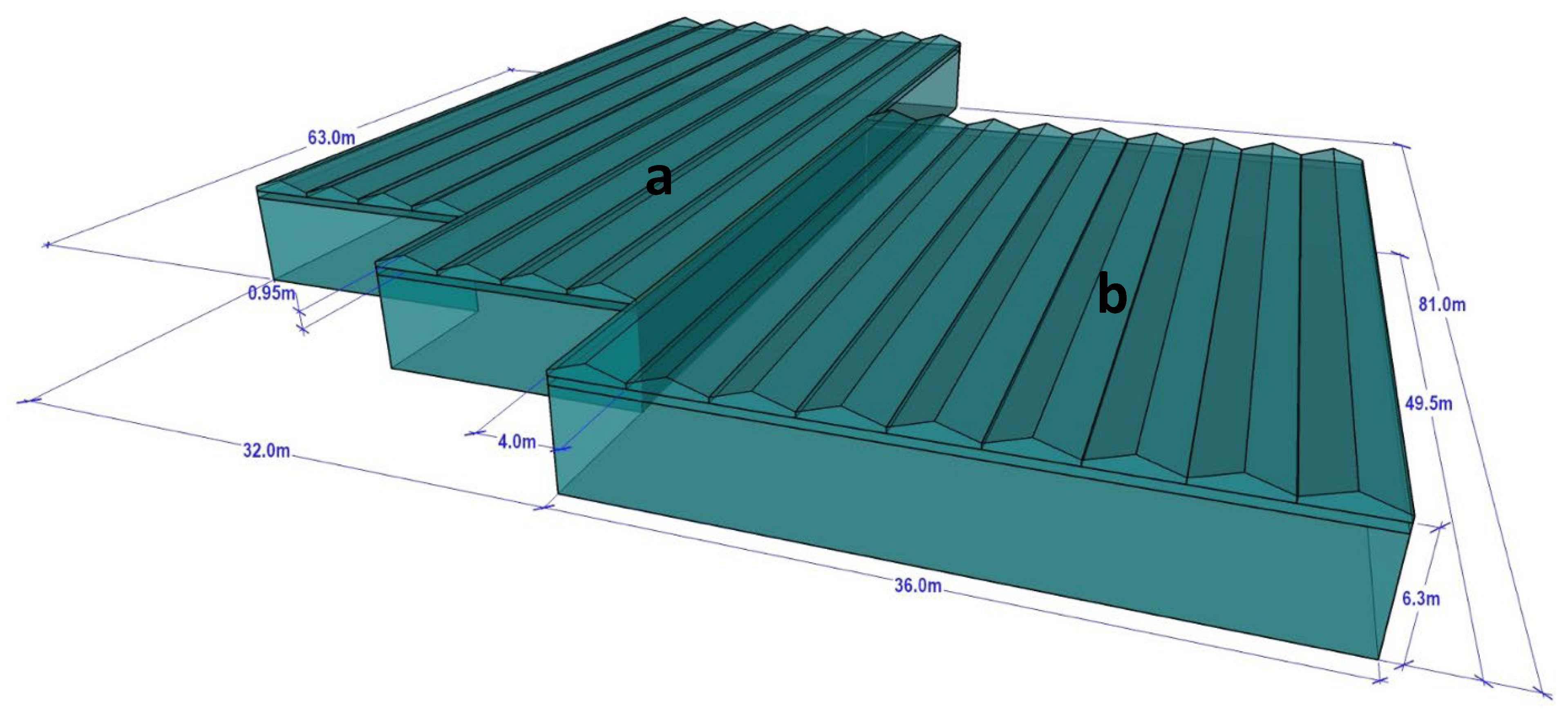
Dynamic simulation of the greenhouse environment in TRNSYS was conducted by linking several components from the TRNSYS library. After connecting the required components, the time steps were specified to run the simulation. Figure 9 shows the simulation studio interface, and a dynamic flowchart of the modelling and simulation procedure is shown in Figure 10. Prior to the simulation, a three-dimensional (3D) greenhouse model was designed using the add-in TRNSYS3D for Google SketchUp (Figure 11). In Google SketchUp, the greenhouse was divided into three zones separated by thermal screens, as shown in Figure 3.

The screens use the same shading device principle as that in a residential building to limit the conductive and radiative heat losses from the greenhouse. Similar to a residential building where the shading device is designed to open or close based on solar radiation, this study controls the thermal screens based on solar radiation using Equations (9) and (10). Equations (9) and (10) are for Tempa and Luxous control, respectively:

$$\mathrm{If} {{\displaystyle \int }}_{T_i<18 °\mathrm{C}}^{SR<200{ \mathrm{Wm}}^{-2}}\mathrm{then} \left(bool=1\right) \mathrm{else} \left(bool=0\right),$$

(9)

$${{\displaystyle \int }}_{T_i<15 °\mathrm{C}}^{SR<150{ \mathrm{Wm}}^{-2}}\mathrm{then} \left(bool=1\right) \mathrm{else} \left(bool=0\right).$$

(10)

The Boolean controller controls the closing (bool = 1) and opening (bool = 0) of the screens; SR is the solar radiation, and T_i is the greenhouse’s internal temperature.

The 3D model was generated in the Intermediate Data Format using Google SketchUp and imported into TRNBuild. TRNBuild was used to define the building orientation and material properties. The TRNBuild database did not include the properties of the greenhouse covering materials and thermal screens used in this study. Therefore, the material properties detailed in Section 2.2 were defined using Berkeley Lab WINDOW 7.4 program, generating a DOE-2 file, and the file was imported into TRNBuild.

The building with airflow (Type 56) was selected in the TRNSYS 18 simulation studio interface to assess the internal greenhouse thermal comfort based on outside weather conditions. The recorded outside weather data were then input into the weather data component (Type 9). The solar radiation recorded was the total horizontal radiation on the horizontal surface. To calculate the direct, diffuse, and reflected solar radiation, Type 16c was linked with Type 9 to accurately account for the solar heat gain of the greenhouse. Type 16c uses different modes to calculate the tilted surface radiation. Rasheed et al. [36] calibrated a TRNSYS model by varying the Type 16c mode. They concluded that mode 2 was the most accurate for modelling the greenhouse internal temperature when the total horizontal radiation was input in Type 9.

Occupancy and equipment were implemented as internal heat gains in TRNBuild and were provided with a schedule using the Type 14 forcing function in the simulation studio. The ASHRAE standard 130 W gain type was chosen for the occupancy, and a radiative and convective power of 0.5 kJh⁻¹ was used for the equipment gain [37]. However, internal gain due to plant evapotranspiration was not considered.

The sensible heat balance of the air within the thermal zones is described as follows:

$${\dot{Q}}_{sens,i}={\dot{Q}}_{surf,i}+{\dot{Q}}_{inf,i}+{\dot{Q}}_{ven,i}+{\dot{Q}}_{g,c,i}+{\dot{Q}}_{cplg,i}+{\dot{Q}}_{solar,i}+{\dot{Q}}_{ISHCC,i},$$

(11)

where ${\dot{Q}}_{sens,i}$ is the sensible heat flux of the zone (kJh⁻¹), ${\dot{Q}}_{surf,i}$ is the convective gain from surfaces (kJh⁻¹), ${\dot{Q}}_{inf,i}$ is the infiltration gains (kJh⁻¹), ${\dot{Q}}_{ven,i}$ is the ventilation gains (kJh⁻¹), ${\dot{Q}}_{g,c,i}$ is the internal convective gains (kJh⁻¹), ${\dot{Q}}_{cplg,i}$ is the gains due to inter-connected air nodes (kJh⁻¹), ${\dot{Q}}_{solar,i}$ is the solar radiation entering an air node through external windows, transformed immediately into a convective gain to the internal air (kJh⁻¹), and ${\dot{Q}}_{ISHCC,i}$ is the solar radiation absorbed on all internal shading devices of the zone transformed immediately into a convective gain to the internal air (kJh⁻¹).

The latent heat flux of the air node is described as follows [37]:

$${\dot{Q}}_{lat,i}=h_v\left[{\dot{m}}_{inf}\left(w_a-w_i\right)+{\dot{m}}_{vent}\left(w_{vent}-w_i\right)+W_g+{\dot{m}}_{ig}\left(w_j-w_i\right)-M_{eff}\left(\frac{w_i-\Delta T}{\Delta T}\right)\right],$$

(12)

where ${\dot{Q}}_{lat,i}$ is the latent energy flux of the zone (kJh⁻¹), $h_v$ is the heat of vaporisation of water (kJkg⁻¹), ${\dot{m}}_{inf}$ is the mass flow rate of infiltration air (kgm⁻³), $w_a$ is the ambient humidity ratio (${\mathrm{kg}}_{water}{\mathrm{kg}}_{air}{}^{-1}$), $w_i$ is the air node humidity ratio (${\mathrm{kg}}_{water}{\mathrm{kg}}_{air}{}^{-1}$), ${\dot{m}}_{vent}$ is the mass flow rate of ventilation air (kg${\mathrm{m}}^{-3}$), $w_{vent}$ is the humidity ratio of ventilation air (${\mathrm{kg}}_{water}{\mathrm{kg}}_{air}{}^{-1}$), $W_g$ is the internal humidity gain (${\mathrm{kg}}_{water}{\mathrm{h}}^{-1}$), ${\dot{m}}_{ig}$ is the mass flow rate due to couplings of two zones (kg${\mathrm{m}}^{-3}$), $w_j$ is the adjacent air node humidity ratio (${\mathrm{kg}}_{water}{\mathrm{kg}}_{air}{}^{-1}$), $M_{eff}$ is the effective moisture capacitance (kg), and $\Delta t$ is the change in time step.

The airflow due to natural ventilation was estimated using TRNFLOW. In TRNFLOW, fans, straight ducts, cracks, and large opening are the different ways of modelling the airflow network. Since the ventilation in the greenhouse involves the opening and closing of the screen, the large opening window was selected. The equation that governs the large opening airflow network is given as follows [38]:

$${\dot{m}}_{1\to 2}=C_d\underset{0}{\overset{H}{{\displaystyle \int }}}\sqrt{2\rho \left(z\right)f_{1\to 2}\left(z\right)}·\sqrt{\frac{{(z·\tan \alpha )}^2·W^2}{{(z·\tan \alpha )}^2+W^2}}·dz$$

(13)

where $\dot{m}$ is the mass flow rate of air (kgh⁻¹), $1\to 2$ is the flow direction from one air node to another, $C_d$ is the discharge coefficient, H is the total height of the window (m), $\rho \left(z\right)$ is the air density (kgm⁻³) at height z, z is the height of the opening (m), $\alpha$ is the angle of opening ($°$), W is the width of rectangular opening (m), and f(z) is the pressure difference at height z (pa).

The thermal zone energy balance is described as follows [39]:

$$C_m\frac{d{T}_m}{dt}=-{\dot{Q}}_{conv,in}-{\dot{Q}}_{lw,in}+\left[{\dot{Q}}_{solg,rad}+{\dot{Q}}_{ig,rad}\right]+{\dot{Q}}_{conv,out}+{\dot{Q}}_{solx}+{\dot{Q}}_{lw,out}+{\dot{Q}}_{cond},$$

(14)

where $T_m$ is the temperature of the masses (°C), $C_m$ is the thermal capacitance of the zone masses (Kj °C⁻¹), ${\dot{Q}}_{conv,in}$ is the convective heat flux between the zone and the inner surface (kJ${\mathrm{h}}^{-1}$), ${\dot{Q}}_{lw,in}$ is the longwave radiation exchange between two inner surfaces (kJ${\mathrm{h}}^{-1}$), ${\dot{Q}}_{solg,rad}$ and ${\dot{Q}}_{ig,rad}$ are the radiative solar and internal gains, respectively (kJ${\mathrm{h}}^{-1}$), ${\dot{Q}}_{conv,out}$ is the convective heat flux between the external surface and ambient (kJ${\mathrm{h}}^{-1}$), ${\dot{Q}}_{solx}$ is the absorbed solar gain on the outside opaque surfaces (kJ${\mathrm{h}}^{-1}$), ${\dot{Q}}_{lw, out}$ is the longwave radiation emitted by the outside surfaces to their surroundings (kJ${\mathrm{h}}^{-1}$), and ${\dot{Q}}_{cond}$ is the heat conduction through the building envelope (kJ${\mathrm{h}}^{-1}$).

Different radiation modes are available for computing the direct and diffuse shortwave and longwave radiations within a thermal zone in the TRNbuild. The radiation modes are explained in the following subsections.

2.3.1. Beam Radiation Distribution

Standard and detailed modes are available for the beam radiation distribution. The standard mode uses a user-defined factor called GEOSURF to distribute beam radiation within a zone. GEOSURF is the fraction of beam radiation that strikes the individual surfaces with a maximum value of 1 per zone. The detailed mode for the beam radiation distribution was used to distribute the solar radiation entering the zone through external windows. An external program, TRNSHD, is used by TRNBuild to generate the shading and insolation matrices required for the detailed mode. However, for beam radiation entering the zone through an adjacent window, GEOSURF was also applied.

2.3.2. Diffuse Radiation Distribution

Standard and detailed modes based on different principles are available for the diffuse radiation distribution. The standard mode is based on the absorption–transmission weighted area ratios for all surfaces, whereas the detailed mode uses the Gebhart factor for shortwave diffuse radiation. An auxiliary program, TRNVFM, based on the view factor matrix is used in the detailed mode.

2.3.3. Longwave Radiation Distribution

Simple, standard, and detailed modes are available for the longwave radiation within a zone. The simple mode is a one-node model with a combined transfer function, assuming a constant convective coefficients and longwave radiation resistance for the heat transfer process.

The standard mode calculates simultaneously the longwave radiation exchange between the surfaces in an air node and the convective heat flux from the inside surfaces to the air node using a star network. This approach uses an artificial temperature of the air node (T_star) to consider simultaneously the energy flow from a wall surface by convection to the air node and radiation to other surfaces. A mathematical description of the internal surface is given in Equations (15)–(17) [40]:

$$R_{star,i}=\frac{1}{Q_{surf,i}}\left(T_{star}-T_i\right),$$

(15)

$$\dot{q_{comb,s,i}=}\dot{q_{c,s,i}}+\dot{q_{r,s,i}},$$

(16)

$$\dot{q_{comb,s,i}}=\frac{1}{R_{equiv,i}·A_{s,i}}\left(T_{s,i}-T_{star}\right),$$

(17)

where $R_{star,i}$ and $R_{equiv,i}$ are the resistance of each surface and the equivalent resistance of all the surfaces (Ohms), respectively, $\dot{q_{c,s,i}}$ is the convective heat flux (kJ${\mathrm{h}}^{-1}$), $\dot{q_{r,s,i}}$ is the radiative heat flux (kJ${\mathrm{h}}^{-1}$), $\dot{q_{comb,s,i}}$ is the combined convective and radiative heat flux (kJ${\mathrm{h}}^{-1}$), $A_{s,i}$ is the inside surface area (m²), and $T_{s,i}$ and $T_i$ are the surface and the equivalent air node temperatures (°C), respectively.

In addition, the total heat transfer at the outside surface is the sum of the convective and radiative heat fluxes calculated from Equations (18)–(21) [37]. The convective heat transfer at the outside surface is complicated due to wind direction, building size, local wind velocity, building surrounding, and building size [40].

$$\dot{q_{comb,s,o}=}\dot{q_{c,s,o}}+\dot{q_{r,s,o}},$$

(18)

$$\dot{q_{c,s,o}}=h_{conv,s,o}\left(T_{a,s}-T_{s,o}\right),$$

(19)

$$\dot{q_{r,s,o}}=\sigma ·{\epsilon }_{s,o}\left(T^4{}_{s,o}-T^4{}_{fsky}\right),$$

(20)

$$T_{fsky}=\left(1-f_{s,sky}\right)·T_{sgrd}-f_{s,sky}·T_{sky},$$

(21)

where $\dot{q_{c,s,o}}$ is the convective heat flux to the outside surface (kJ${\mathrm{h}}^{-1}$), $\dot{q_{r,s,o}}$ is the radiative heat flux to the outside surface (kJ${\mathrm{h}}^{-1}$), $\dot{q_{comb,s,o}}$ is the combined convective and radiative heat flux to the outside surface (kJ${\mathrm{h}}^{-1}$), $h_{conv,s,o}$ is the convective heat transfer coefficient at the outside surface, $T_{a,s}$ is the outside surface temperature (°C), $T_{s,o}$ is the ambient temperature (°C), ${\epsilon }_{s,o}$ is the longwave emissivity of the outside surface from the WINDOW library, $\sigma$ is the Stefan–Boltzmann constant, $T_{fsky}$ is the fictive temperature difference between the ground and sky (°C), $f_{s,sky}$ is the view factor of the sky, $T_{sgrd}$ is the fictive ground temperature (°C), $1-f_{s,sky}$ is the view factor of each external surface, and $T_{sky}$ is the fictive sky temperature (°C).

Compared with the standard mode, the artificial star node is not considered in the detailed mode because the convective heat flux is calculated separately. The detailed mode used the Gebhart factor ($G_{ir,1-2}$) for longwave radiation exchange, considering multi-reflection from surfaces. The Gebhart factor is the fraction of emission from surface $A_1$ that reaches surface $A_2$ and is absorbed. $G_{ir,1-2}$ includes all paths (direct and multiple reflections) to reach $A_2$. The Gebhart matrix for longwave radiation is given by Equation (22):

$$G_{ir}={\left(I-F{\rho }_{ir}\right)}^{-1}F{\epsilon }_{ir},$$

(22)

where ${\rho }_{ir}$ and ${\epsilon }_{ir}$ are diagonal matrices describing reflectivity and emissivity, I is an identity matrix, and F is the view factor, which is the fraction of diffusely radiated energy leaving surface 1 that is incident on surface 2; ‘ir’ represents the longwave range of the radiation spectrum (infrared).

The auxiliary matrix $(G_{ir}{}^{*})$, given by Equation (23), was introduced to determine the longwave radiation (${\dot{Q}}_{ir}$) in the enclosure:

$$G_{ir}{}^{*}=\left(I-G_{ir}{}^T\right)A\epsilon \sigma ,$$

(23)

where $G_{ir}{}^T$ is the transpose of $G_{ir}$, A is the diagonal matrix describing the surface areas, $\sigma$ is the Stefan–Boltzmann constant, and $\epsilon$ is the longwave emissivity.

Then,

$${\dot{Q}}_{ir}=G_{ir}{}^{*}{T}^4,$$

(24)

where T is the temperature vector of the enclosure.

Considering that thermal screens and roofs are opened during the day to harness solar radiation, the effects of the beam and diffuse radiation modes are assumed to be negligible in greenhouses compared with residential buildings. However, during the night, the thermal screens and roofs are fully closed when energy is supplied to the conditioned zone of the greenhouse, and the properties of the thermal screens and covering materials determine the conditions of other zones. Therefore, different longwave radiation exchange modes impact the thermal comfort of the greenhouse.

The simple and standard longwave radiation modes cannot consider radiation exchange over more than one air node. The greenhouse was modelled as a single air node per zone as shown in Figure 11, to investigate the effects of the three longwave radiation modes. The shape of a building must be convex and closed to generate its view factor matrix for the detailed longwave radiation mode. Farm A is a concave-shaped greenhouse, and farm B is a convex-shaped greenhouse (Figure 12). Consequently, for farm A, the simple and standard longwave radiation models were utilised, whereas for farm B, the simple, standard, and detailed modes were adopted.

2.4. BES Model Validation

The proposed BES model was validated using the Nash–Sutcliffe efficiency coefficient (NSE) represented by Equation (25). This coefficient quantifies the fit of the experimentally measured data with the simulated data in a 1:1 plot. Its value ranges from $-\infty$ to 1, with values closer to 1 indicating substantial predictive potential of the model:

$$\mathrm{NSE}=1-[\frac{{{\displaystyle \sum }}_{i=0}^n{\left(X_i{}^{exp}-X_i{}^{sim}\right)}^2}{{{\displaystyle \sum }}_{i=0}^n{\left(X_i{}^{exp}-X_i{}^{mean}\right)}^2}],$$

(25)

where $X_i{}^{exp}$ is the experimentally measured data, $X_i{}^{sim}$ is the simulated data, and $X_i{}^{mean}$ is the mean of the experimentally measured data.

2.5. Sensitivity Analysis

A sensitivity analysis was performed to determine the impact of the longwave radiation modes on the total monthly heating demand. In mathematical modelling, sensitivity analysis quantifies the effects of several independent variables on the dependent variable under a specific condition, and the sensitivity coefficient (SC) is a dimensionless factor widely used to characterise the error assessment. The simplest form of the sensitivity coefficients for comparative energy studies, as given by Lam and Hui [41], is presented in Equation (26):

$$\mathrm{SC}=\frac{\Delta \mathrm{OP}}{\Delta \mathrm{IP}},$$

(26)

where OP is the output, and IP is the input.

In addition to the radiation modes, several other factors, including infiltration, moisture change, and capacitance, affect the heating requirement of a greenhouse in the BES model. Rather than changing these parameters, the output of the heating requirements from the radiation modes is considered as the OP, whereas the measured heating consumption from the greenhouse was considered as the IP.

3. Results and Discussion

3.1. Radiometric Properties of the Novel Greenhouse Materials

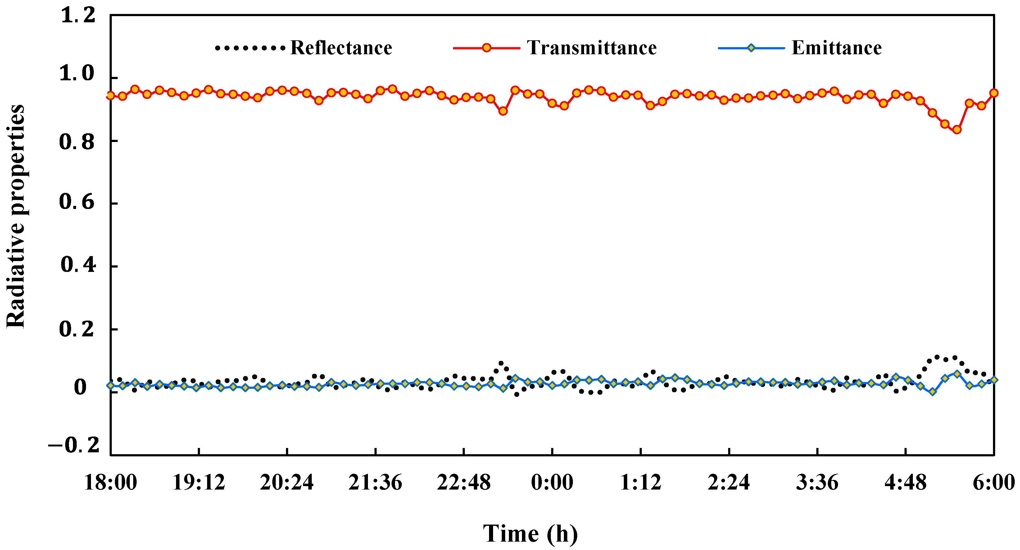
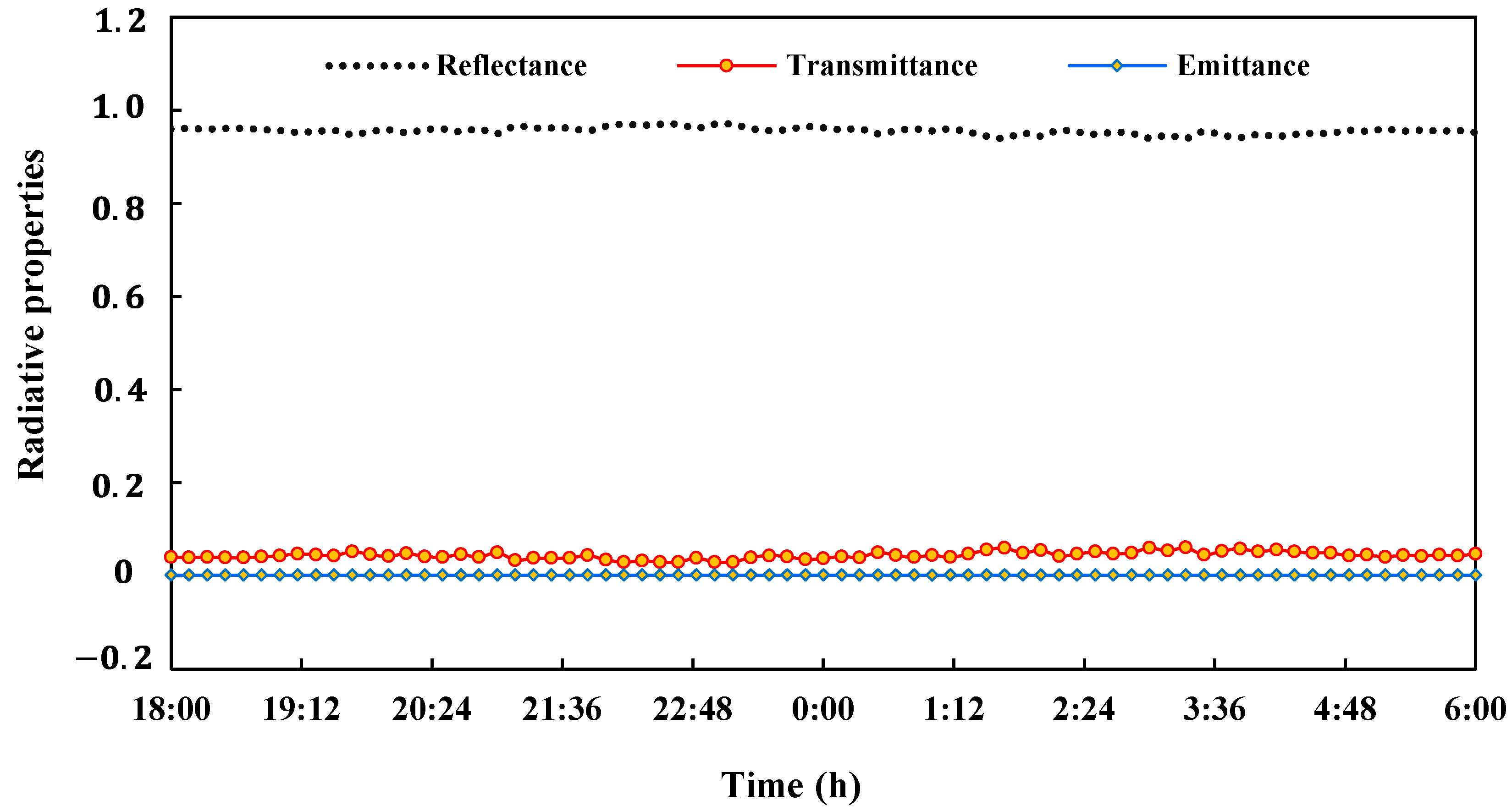
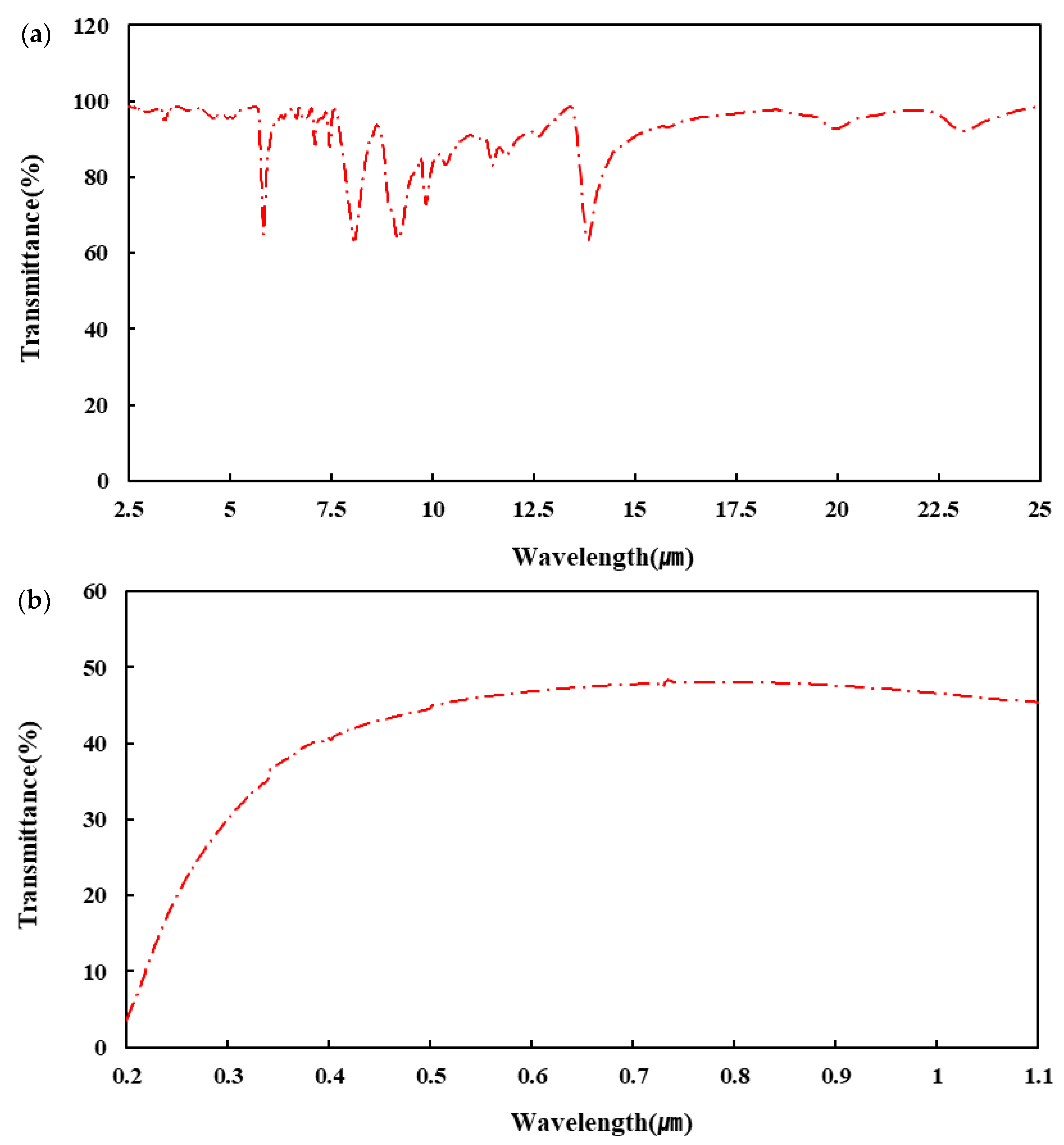
The experiment based on RBM was conducted for several nights, and the results were compared with those by spectrophotometry. Figure 13 and Figure 14 show the longwave radiative properties of the fluorine film and Obscura measured from 18:00 to 06:00 based on RBM. The reflectance, transmittance, and emittance of the fluorine film were 0.43, 0.94, and 0.02, respectively. The reflectance, transmittance, and emittance of Obscura were 0.96, 0.001, and 0.045, respectively. Because the Obscura has approximately zero transmittance in the longwave spectrum, spectrophotometry was used only for the fluorine film within the waveband of 2.5 to 25 μm (Figure 15a). The longwave transmittance result by spectrophotometry was the same as that by RBM. The consistency of the results using the two methods validates the accuracy in the determination of the radiative properties of the materials used in the BES modelling (

Table 4. Properties of the novel greenhouse materials.

Cover Characteristics	Fluorine Film	Obscura
Thickness (mm)	0.08	0.34
Solar transmittance (front)	0.92	0.01
Solar transmittance (back)	0.92	0.01
Solar reflectance (front)	0.06	0.64
Solar reflectance (back)	0.06	0.64
Visible radiation transmittance (front)	0.92	0.01
Visible radiation transmittance (back)	0.92	0.01
Visible radiation reflection (front)	0.06	0.64
Visible radiation reflection (back)	0.06	0.64
Thermal radiation transmittance	0.94	0.001
Thermal radiation emission (front)	0.02	0.045
Thermal radiation emission (back)	0.03	0.045
Thermal conductivity (Wm−1K−1)	0.15	0.35
Infiltration (m3h−1m2)	-	-

).

The diffuse shortwave transmittance of the fluorine film, measured using an ultraviolet-visible spectrophotometer (Jasco V-730), is shown in Figure 15b. The measured diffuse transmittance is 45.86%. However, owing to the limitations of spectrophotometry, the total transmittance was measured using a haze meter. The total transmittance was 92.49% with the beam and diffuse transmissions contributing to 46.74% and 45.75%, respectively. The solar transmittance of the fluorine film indicates that it transmits more than 90% of the shortwave radiation, which is vital for plant growth. This value is higher than the transmittance of the commonly used greenhouse covering materials, polyethylene (71%) [34] and HG (89%) [33]. The solar transmittance obtained is similar to the longwave transmittance; this does not agree with Choab et al. [42], who recommended high and low transmittances in the shortwave and longwave spectra, respectively, for covering materials. However, the installed thermal screens have very low transmittance in the longwave spectrum (Tempa, 5%; Luxous, 33%) to limit heat loss before transmission through the film.

3.2. Comparison of Results of the TRNSYS Model with the Experimental Measurements

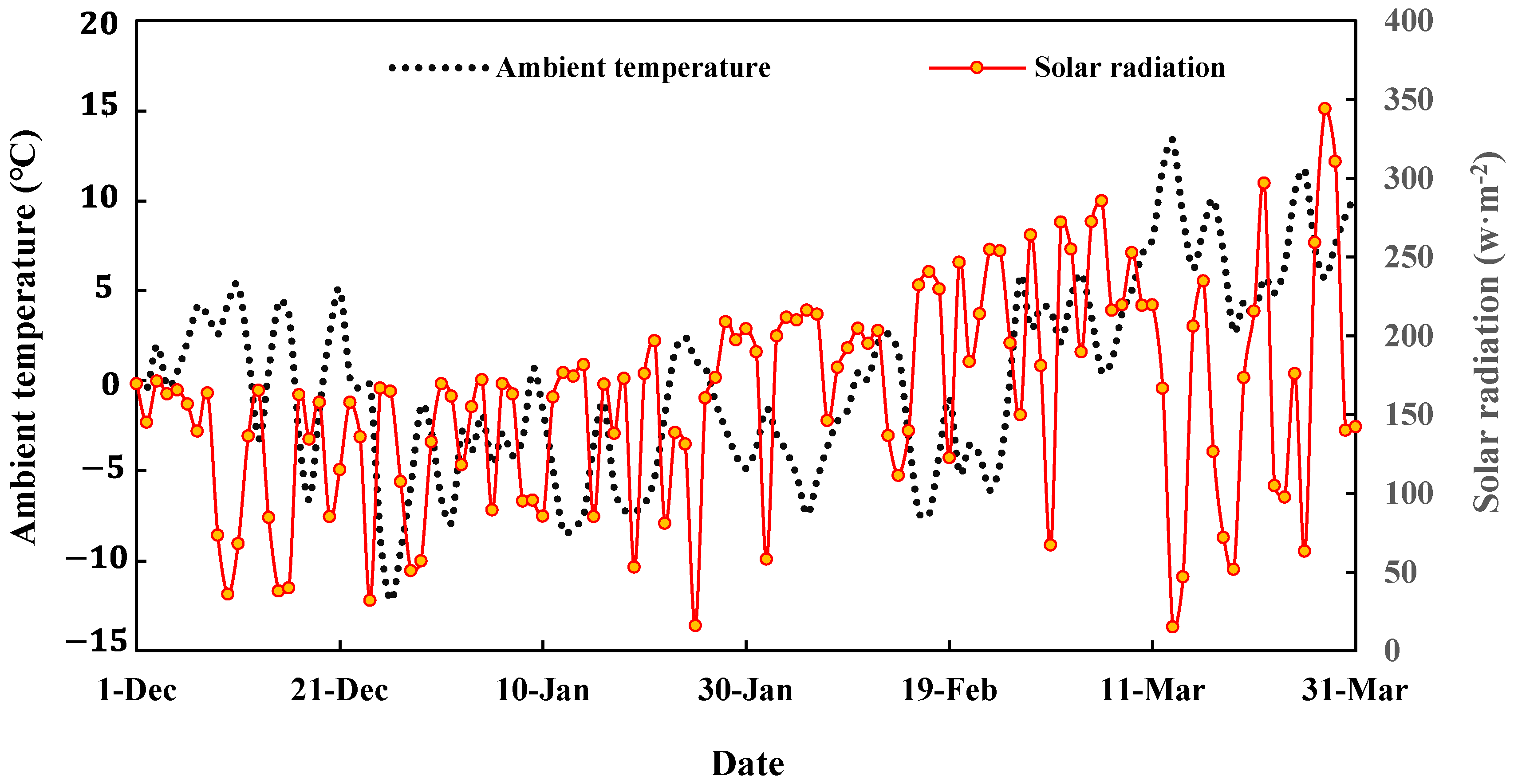
The daily average outside temperature and average solar radiation on the horizontal surface are shown in Figure 16. The dataset represents meteorological conditions in Yeoju, South Korea, during the winter season between December 2021 and March 2022. The lowest and the highest hourly temperatures (−17.8 °C and 20.2 °C, respectively) were recorded on 26 December 07:00 and 12 March 15:00, respectively. For temperature, the daily average low (of −12.2 °C) and high (of 13.3 °C) were recorded on 26 December and 13 March, respectively. The maximum hourly solar radiation (1103.6 ${\mathrm{Wm}}^{-2}$) was on 28 March, 12:00. Both minimum and maximum daily average solar radiations (15.1 ${\mathrm{Wm}}^{-2}$ and 344 ${\mathrm{Wm}}^{-2}$, respectively) were recorded in March. The coldest month was January, with a monthly average temperature of −3.6 °C.

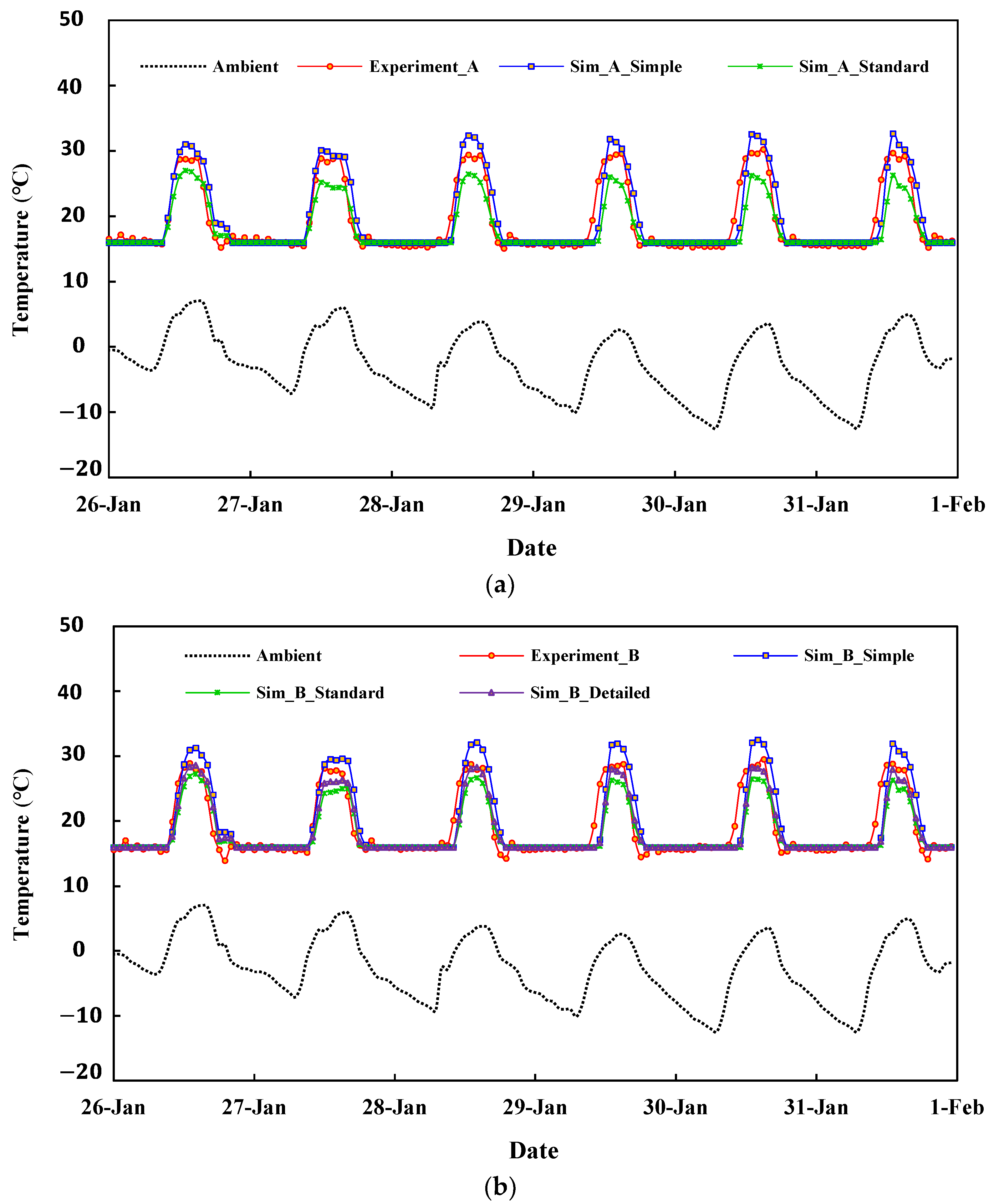
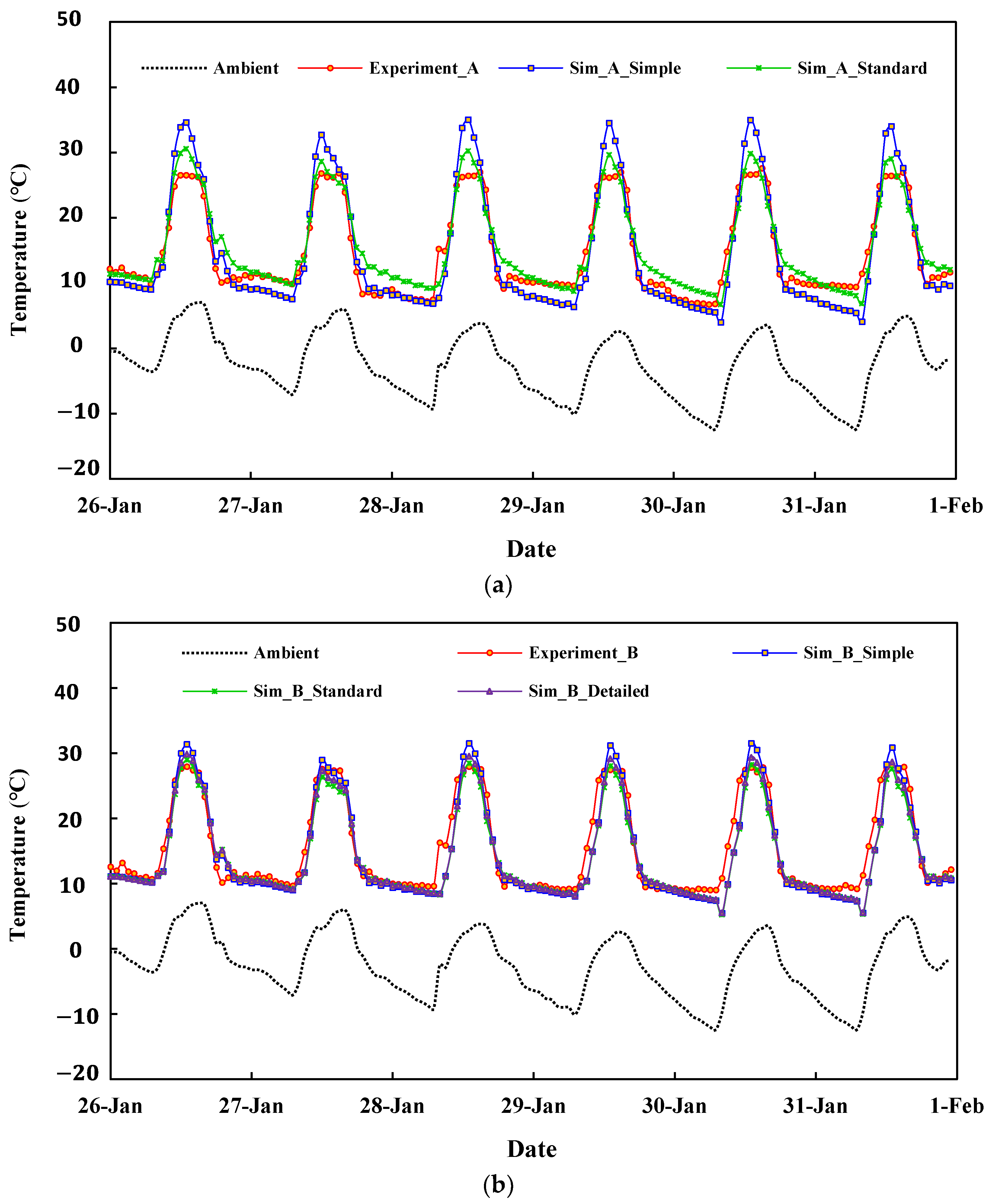
The simulated internal temperatures in the different zones for both farms were compared with the experimentally measured temperatures of the greenhouse. Because the daily greenhouse conditioning is approximately the same during the winter season, only a few days of the analysis are discussed. Figure 17 shows the simulated zone 1 temperatures compared with the experimentally measured temperatures from 26 to 31 January. On most days, the greenhouse’s experimental daytime temperature was approximately 30 °C for both the farms. For farm A, the simulated daytime temperatures differ from the observed temperatures by a maximum of 3.0 °C (above the observed temperature) and 3.0 °C (below the observed temperature) for the simple and standard modes, respectively. For farm B, the simulated maximum daytime temperatures differ from the observed temperatures by a maximum of 3.0 °C (above the observed temperature), 2.3 °C (below the observed temperature), and 0.94 °C (below the observed temperature) for the simple, standard, and detailed modes, respectively. The simple and standard modes over-predicted and under-predicted the daytime temperatures, respectively, for both greenhouses. The controlled simulated night temperature for the three modes was 15 °C. So, it was not possible to determine the impact of the modes on the night temperature in zone 1. The calculated NSE values for farm A were 0.85 and 0.78 for the simple and standard modes, respectively. The calculated NSE values for farm B were 0.73, 0.78, and 0.83 for the simple, standard, and detailed modes, respectively.

Figure 18 shows the simulated zone 2 temperatures compared with the experimentally measured temperatures. The thermal screens placed between zones 1 and 2 caused an approximately 5 °C temperature difference between the two zones during the night when zone 1 was being heated. For farm A, the simple and standard modes over-predicted the daytime temperatures by a maximum of 8 °C and 3 °C, respectively. Similarly, for farm B, the simulated daytime temperatures differ from the observed temperatures by a maximum of 3.4 °C, 1.72 °C, and 0.8 °C above the observed temperature for the simple, standard, and detailed modes, respectively. However, the simple and standard modes under-predicted the night temperature by a maximum of 5.34 °C and 2.54 °C, respectively, in Farm A. By contrast, for farm B, the maximum difference of the simple, standard, and detailed modes was 3.5 °C, 3.7 °C, and 3.4 °C below the observed night temperatures, respectively. The calculated NSE values for farm A were 0.79 and 0.89 for the simple and standard modes, respectively. The calculated NSE values for farm B were 0.89, 0.88, and 0.9 for the simple, standard, and detailed modes, respectively.

Figure 19 shows the simulated zone 3 temperatures compared with the experimentally measured temperatures. The thermal screens placed between zones 2 and 3 caused an 8 °C temperature difference between the two zones during the night. This temperature difference is higher than between Zone 1 and 2 owing to the low transmissive properties of Tempa compared with Luxous. The average temperature difference between zone 3 and the ambient was 10 °C. The calculated NSE values for farm A were 0.91 and 0.93 for the simple and standard modes, respectively. The calculated NSE values for farm B were 0.92, 0.91, and 0.92 for the simple, standard, and detailed modes, respectively.

As the NSE values for all radiation modes were higher than 0.5, the BES model was valid, and the standard and detailed models were recommended for predicting the internal greenhouse temperature for concave and convex-shaped greenhouses. However, the user-defined emissivities of the surface for longwave radiation can only be handled using a detailed model. Therefore, a detailed model should be adopted to accurately model the internal greenhouse temperature.

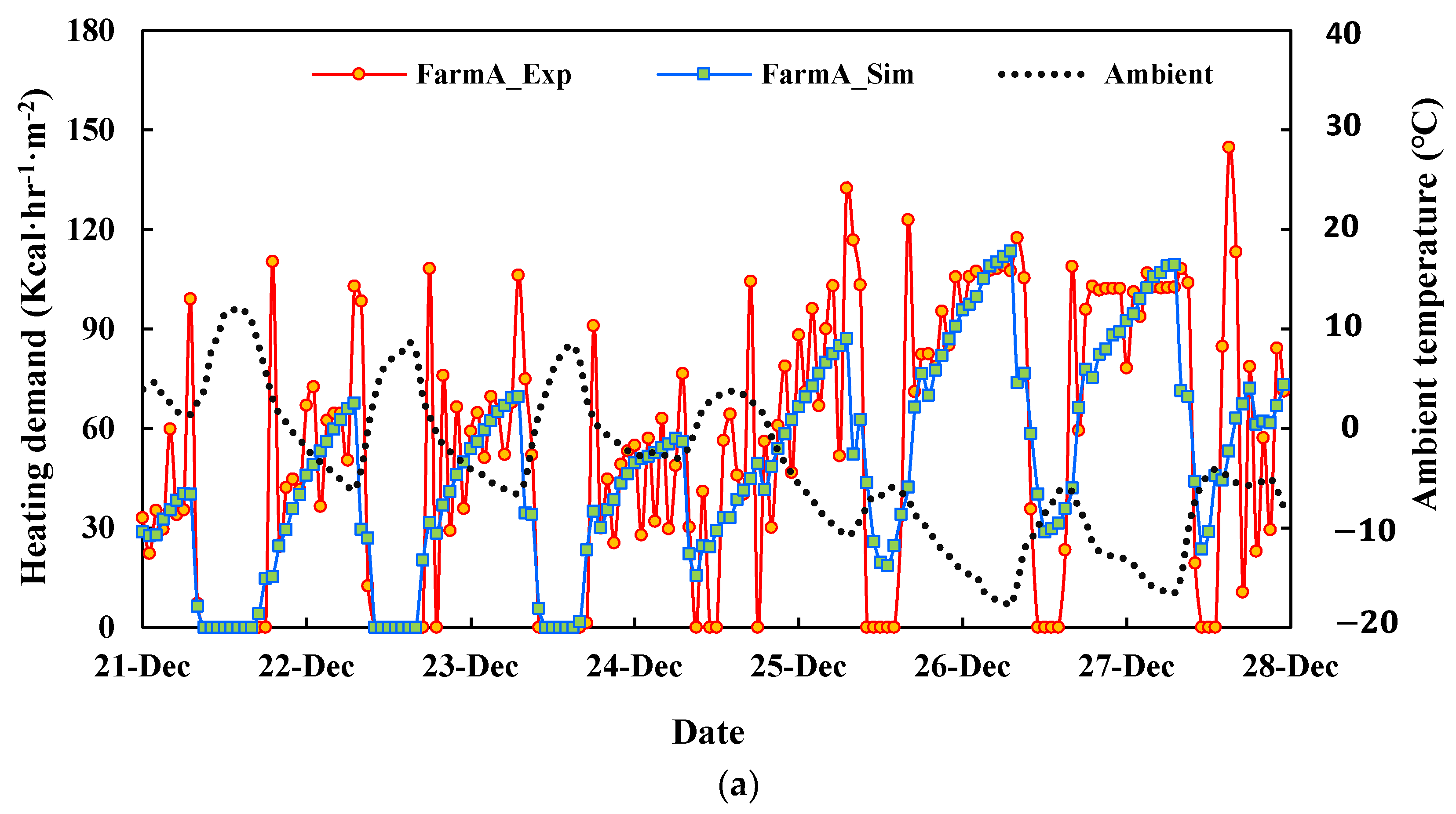
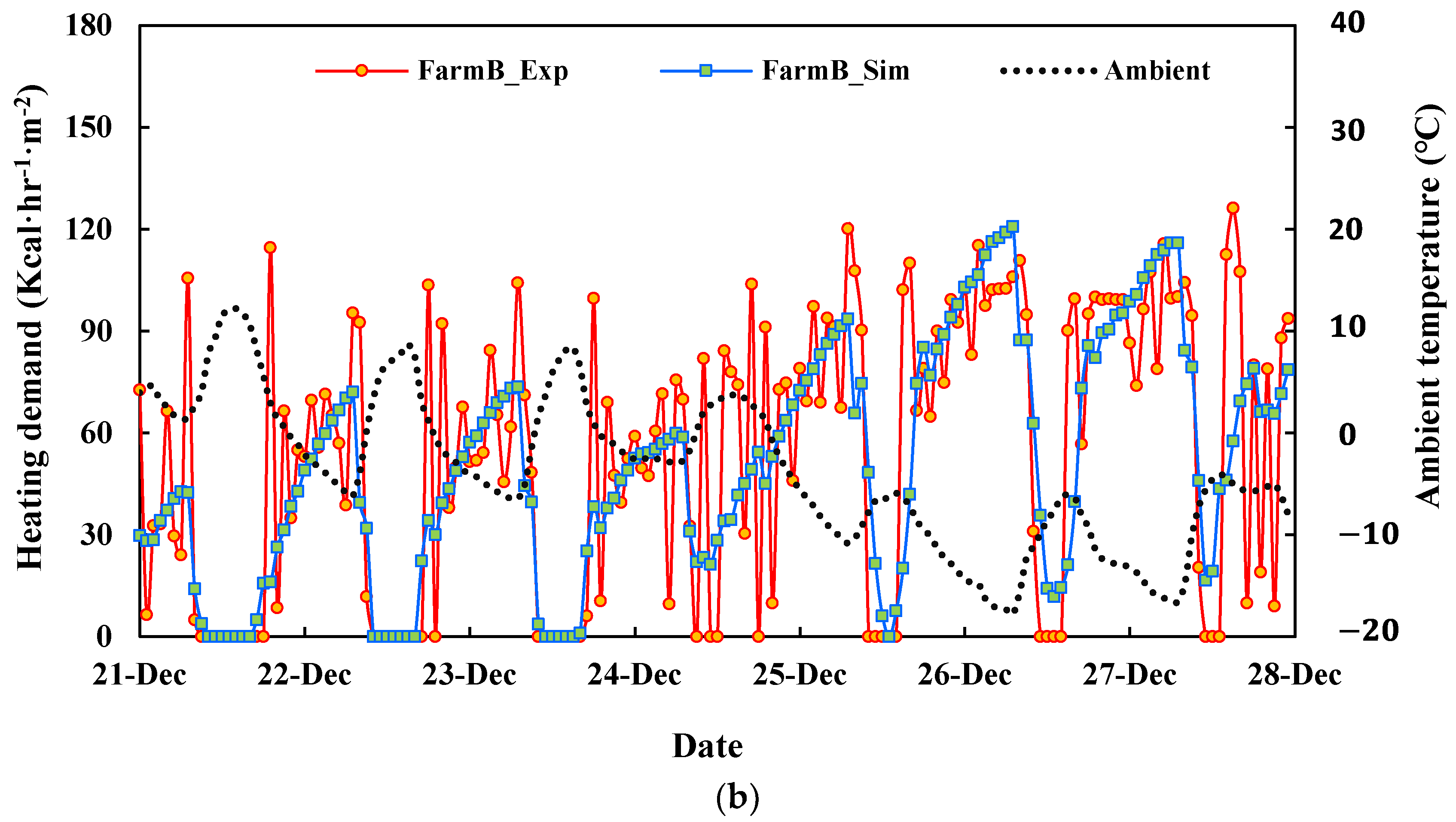
Because the overall performance of the standard and detailed radiation modes for farms A and B was superior, both were used to analyse the heating demand of the two greenhouses. However, the maximum heating demand varied for the different radiation modes (

Table 5. Heating loads using TRNSYS for different radiation modes.

Farm	Greenhouse Set Point Temperature (°C)	Maximum Outside Temperature (°C)	Greenhouse Heating Area (m2)	Radiation Mode	Maximum Heating Load (kcal/hm2)
A	15	−17.8	2160	Simple	101.3
				Standard	113.5
B	15	−17.8	1782	Simple	116.4
				Standard	123.4
				Detailed	120.7

). Figure 20 compares the simulated heating demand with the experimental energy consumption during the period of the lowest ambient temperature from 21 to 27 December 2021. There were significant hourly changes between the simulated and measured results owing to the transient state of the experimental greenhouse and the intermittent application of the energy control systems. The maximum heating loads for farms A and B were 113.5 kcal/hm² and 120.7 kcal/hm², respectively, on 26 December when the ambient temperature (−17.8 °C) was minimum and the greenhouse set point temperature was 15 °C. For the same greenhouse with similar hybrid heat pump systems using geothermal sources and solar heat, Jeon et al. [43] designed a greenhouse (1015 m²) with a maximum heating load of 148.8 kcal/hm² for the lowest ambient temperature of −19 °C and greenhouse set point temperature of 23 °C. The simulated maximum heating demands for both the farms with the thermal screens were high compared with Rasheed et al. [23], who obtained 109.9 kcal/hm², 98 kcal/hm², and 81.3 kcal/hm² using single-, double-, and triple layered-thermal screens, respectively, for a greenhouse floor area of 7572.6 m². However, the simulated heating demand was lower than that of a greenhouse with a floor area of 391.2 m² and with a maximum heating load of 250 kcal/hm² [44]. This trend indicates that greenhouse heating demand per square meter decreases with increasing floor area. Heat is lost through all greenhouse surfaces, including walls, roofs, and floors, and the amount of heat lost per square meter increases as the wall-to-total surface area ratio increases.

The total daily heating demand was compared with the total daily energy consumed for BES model performance. The maximum heating demand was on 19 January (farm A: 3547.8 Mcal/day, and farm B: 3118.9 Mcal/day) when the daily average temperature was −7.3 °C. In the study by Ahamed et al. [22] using the CSGHEAT models with MATLAB, the average daily heating requirement in a CSG integrated with thermal screens was 900 MJ/day (215.2 Mcal/day). The CSG heating area was 210 m². This is approximately ten times lower than that of the experimental glass greenhouse. The calculated NSE values for farms A and B were 0.89 and 0.9, respectively, indicating the model’s ability to predict the greenhouse energy load.

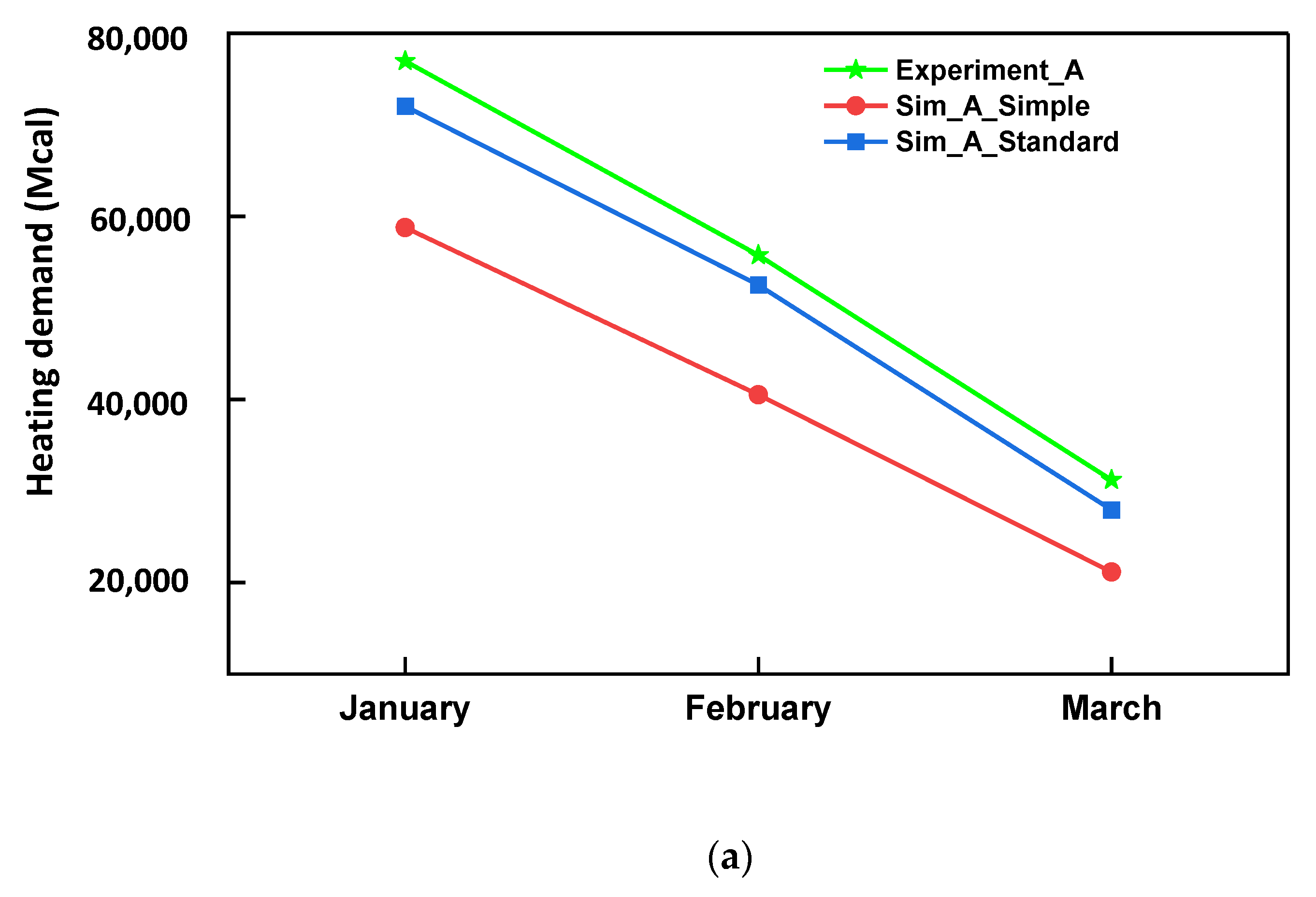
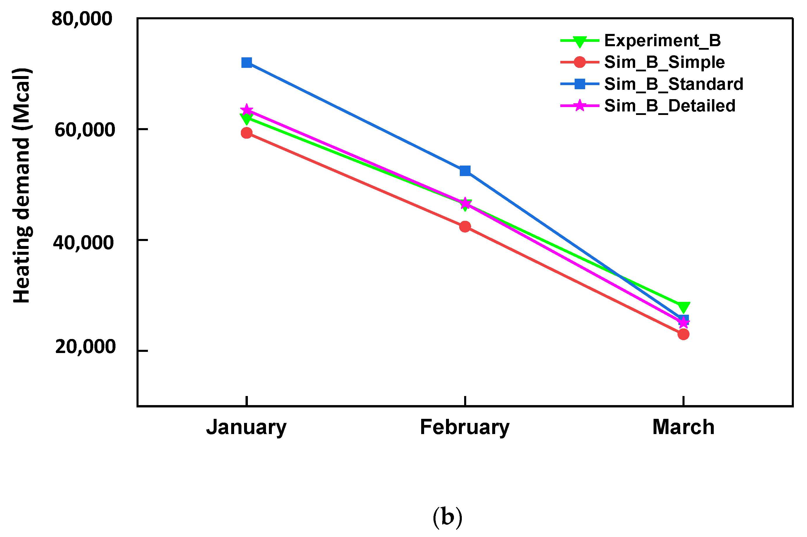
Figure 21 shows the monthly heating demands predicted by the radiation modes and the experimental heating energy consumption. The radiation modes affected the simulated heating requirement of the greenhouse. The monthly heating demand predicted by the simple and standard radiation modes for farm A matched the experimental measurements with deviations within 27.7% and 7.6%, respectively. The monthly heating loads predicted by the simple, standard, and detailed radiation modes for farm B were similar to the experimental measurements with deviations within 10.5%, 6.7%, and 2.9%, respectively. For both greenhouses, the monthly heating requirements predicted by the simple mode were less than the experimental measurements. However, the standard mode under- and over-predicted the monthly heating requirements in farms A and B, respectively.

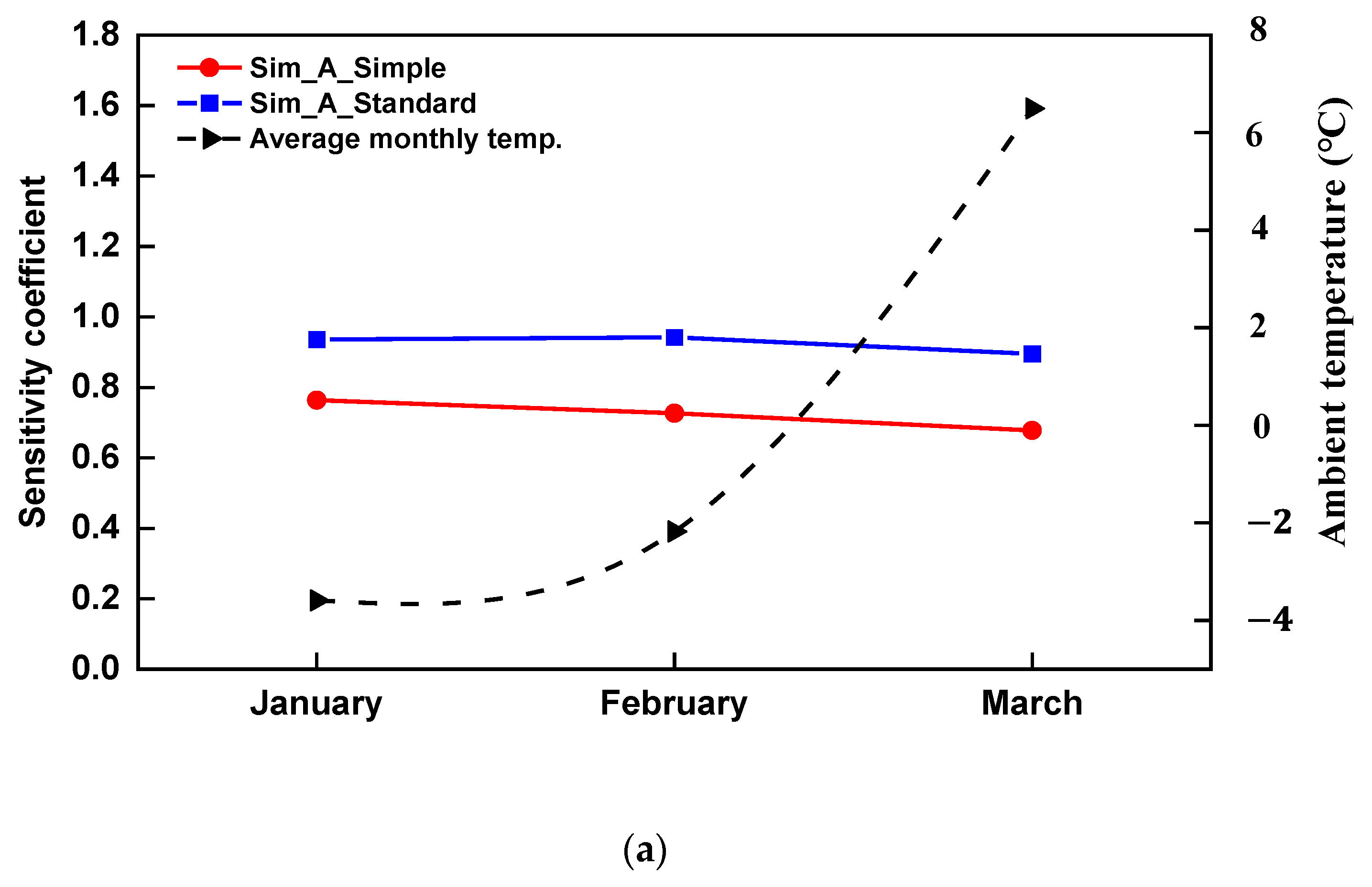
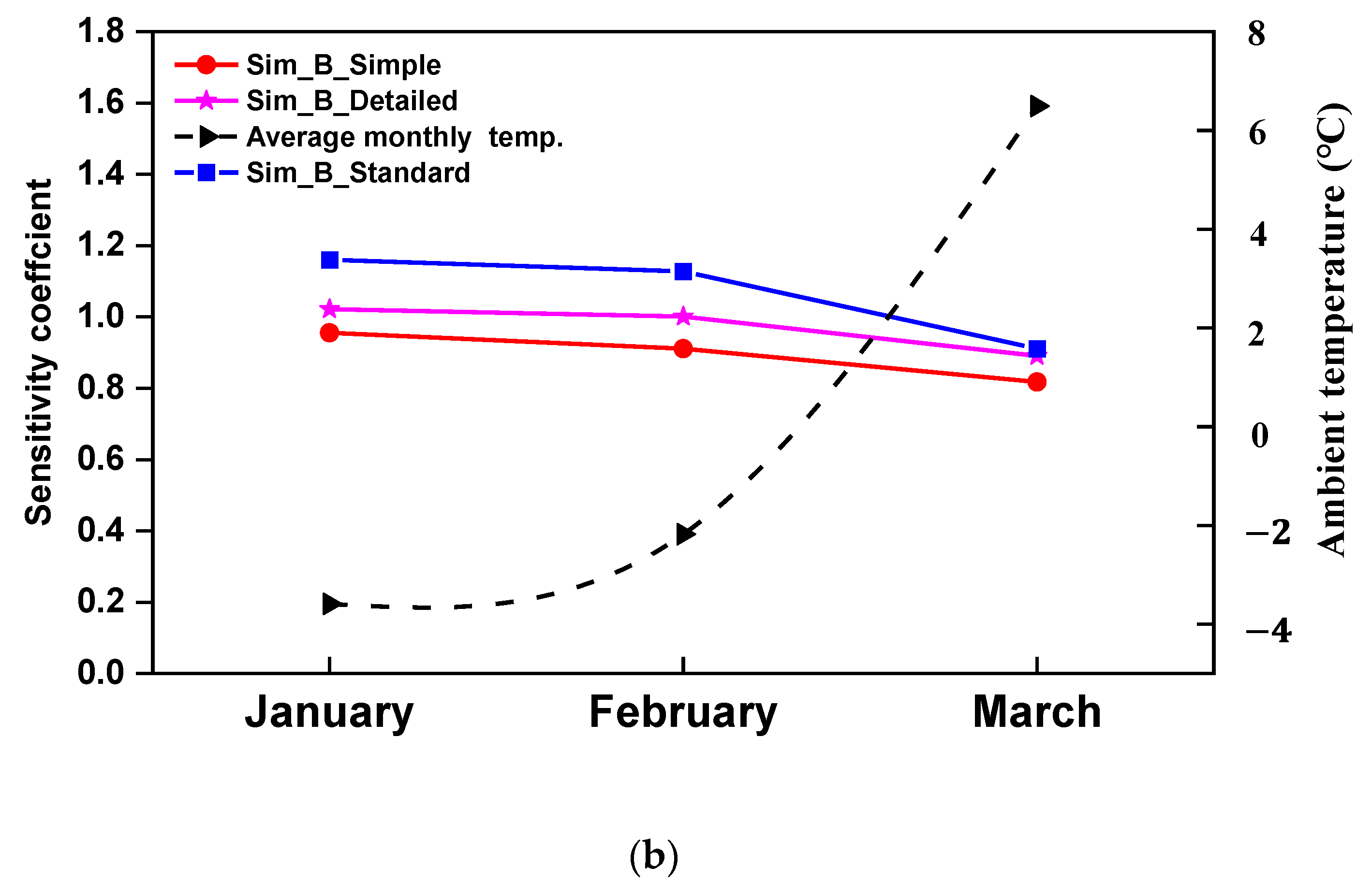
Figure 22 shows the SC for both the farms. The simple and standard modes for farm A had an average SC of 0.7 and 0.9, respectively, whereas the simple, standard, and detailed modes for farm B had an average SC of 0.9, 1.1, and 1.0, respectively. In addition, for farm B, as the monthly ambient temperature increases, the heating demand predicted by the standard and detailed modes converged, indicating that the differences in the predictions between the radiation modes were more pronounced during cold months for a convex-shaped greenhouse.

3.3. Limitation of the Study and Future Work

The proposed BES model has some limitations. Firstly, three weather data (windspeed, wind direction, and ambient pressure) used in the simulation were downloaded at a neighbouring station, 18 km from the experimental greenhouse. The results obtained could lead to a slight variation if the model is to be adapted for year-round simulation, as the greenhouse solely depends on wind forces for natural ventilation in the summer. However, the division of the greenhouse based on the geometry shows the variation in the radiation mode on the internal temperature and heating demand of the greenhouse. More so, in the absence of on-site data, several researchers have used neighbouring stations weather data. Choi et al. [45] had studied the windspeed trend of 31 KMA stations from 1985–2019 and concluded that the average wind speed in Korea does not change that much, while Kim et al. [46] developed a TRNSYS model for Jincheon using Cheongju weather data, 23.9 km away from Jincheon. Secondly, the planted crops were not considered in the simulation. Although they are the most important factor in greenhouse simulation [47], the absence of a stand-alone component in TRNSYS limited their consideration in our study.

The present TRNSYS model could only access the greenhouse thermal performance based on radiation modes without including the internal heat gains due to evapotranspiration from the crop. Modified crop models to calculate the latent mass flow and latent power due to the presence of crop will be implemented in future.

4. Conclusions

The greenhouse industry is faced with challenges to increase production and reduces the use of resources. Mathematical modelling has been seen as alternative to identify potential solutions. In this study, TRNSYS was used to investigate the thermal performance of a glass greenhouse integrated with movable thermal screens. For the novel greenhouse covering materials and thermal screens considered in the study, the thermo-physical, aerodynamics, and radiative properties were experimentally determined for accurate BES modelling. The internal greenhouse temperature and heating demand were simulated using different longwave radiation modes, and the simulated results were validated using transient experimental data. The performances of the standard and detailed modes were superior in concave- and convex-shaped greenhouses as the radiation modes were sensitive to ambient temperature. The findings of this study will aid greenhouse growers, researchers, and engineers in selecting the appropriate longwave radiation mode for modelling the thermal performance of a greenhouse based on the geometry of the greenhouse.

References

1. Baudoin, W.; Nono-Womdim, R.; Lutaladio, N.; Hodder, A.; Castilla, N.; Leonardi, C.; De Pascale, S.; Qaryouti, M. Cultural Practices and Environment. In Hobby Hydroponics; CRC Press: Boca Raton, FL, USA, 2013; pp. 42–55. ISBN 9789251076491. [Google Scholar]
2. Akpenpuun, T.D.; Na, W.H.; Ogunlowo, Q.O.; Rabiu, A.; Adesanya, M.A.; Addae, K.S.; Kim, H.T.; Lee, H.-W. Effect of Glazing Configuration as an Energy-Saving Strategy in Naturally Ventilated Greenhouses for Strawberry (Seolhyang Sp.) Cultivation. J. Agric. Eng. 2021, 52, 1177. [Google Scholar] [CrossRef]
3. Ogunlowo, Q.O.; Akpenpuun, T.D.; Na, W.H.; Rabiu, A.; Adesanya, M.A.; Addae, K.S.; Kim, H.T.; Lee, H.W. Analysis of Heat and Mass Distribution in a Single-and Multi-Span Greenhouse Microclimate. Agriculture 2021, 11, 891. [Google Scholar] [CrossRef]
4. Banakar, A.; Montazeri, M.; Ghobadian, B.; Pasdarshahri, H.; Kamrani, F. Energy Analysis and Assessing Heating and Cooling Demands of Closed Greenhouse in Iran. Therm. Sci. Eng. Prog. 2021, 25, 101042. [Google Scholar] [CrossRef]
5. Mazzeo, D.; Baglivo, C.; Panico, S.; Congedo, P.M. Solar Greenhouses: Climates, Glass Selection, and Plant Well-Being. Sol. Energy 2021, 230, 222–241. [Google Scholar] [CrossRef]
6. Akpenpuun, T.D.; Na, W.H.; Ogunlowo, Q.O.; Rabiu, A.; Adesanya, M.A.; Addae, K.S.; Kim, H.T.; Lee, H.W. Effect of Greenhouse Cladding Materials and Thermal Screen Configuration on Heating Energy and Strawberry (Fragaria Ananassa Var. “Seolhyang”) Yield in Winter. Agronomy 2021, 11, 2498. [Google Scholar] [CrossRef]
7. Baglivo, C.; Mazzeo, D.; Panico, S.; Bonuso, S.; Matera, N.; Congedo, P.M.; Oliveti, G. Complete Greenhouse Dynamic Simulation Tool to Assess the Crop Thermal Well-Being and Energy Needs. Appl. Therm. Eng. 2020, 179, 115698. [Google Scholar] [CrossRef]
8. Zhang, Y.; Gauthier, L.; De Halleux, D.; Dansereau, B.; Gosselin, A. Effect of Covering Materials on Energy Consumption and Greenhouse Microclimate. Agric. For. Meteorol. 1996, 82, 227–244. [Google Scholar] [CrossRef]
9. Rasheed, A.; Na, W.H.; Lee, J.W.; Kim, H.T.; Lee, H.W. Optimization of Greenhouse Thermal Screens for Maximized Energy Conservation. Energies 2019, 12, 3592. [Google Scholar] [CrossRef] [Green Version]
10. Shukla, A.; Tiwari, G.N.; Sodha, M.S. Thermal Modeling for Greenhouse Heating by Using Thermal Curtain and an Earth-Air Heat Exchanger. Build. Environ. 2006, 41, 843–850. [Google Scholar] [CrossRef]
11. Ahamed, M.S.; Guo, H.; Tanino, K. Energy Saving Techniques for Reducing the Heating Cost of Conventional Greenhouses. Biosyst. Eng. 2019, 178, 9–33. [Google Scholar] [CrossRef]
12. Rasheed, A.; Lee, J.W.; Lee, H.W. Development of a Model to Calculate the Overall Heat Transfer Coefficient of Greenhouse Covers. Spanish J. Agric. Res. 2017, 15, e0208. [Google Scholar] [CrossRef] [Green Version]
13. Guo, Y.; Zhao, H.; Zhang, S.; Wang, Y.; Chow, D. Modeling and Optimization of Environment in Agricultural Greenhouses for Improving Cleaner and Sustainable Crop Production. J. Clean. Prod. 2021, 285, 124843. [Google Scholar] [CrossRef]
14. Lee, S.Y.; Lee, I.B.; Lee, S.N.; Yeo, U.H.; Kim, J.G.; Kim, R.W.; Decano-Valentin, C. Dynamic Energy Exchange Modelling for a Plastic-Covered Multi-Span Greenhouse Utilizing a Thermal Effluent from Power Plant. Agronomy 2021, 11, 1461. [Google Scholar] [CrossRef]
15. Zhang, G.; Ding, X.; Li, T.; Pu, W.; Lou, W.; Hou, J. Dynamic Energy Balance Model of a Glass Greenhouse: An Experimental Validation and Solar Energy Analysis. Energy 2020, 198, 117281. [Google Scholar] [CrossRef]
16. Baneshi, M.; Gonome, H.; Maruyama, S. Wide-Range Spectral Measurement of Radiative Properties of Commercial Greenhouse Covering Plastics and Their Impacts into the Energy Management in a Greenhouse. Energy 2020, 210, 118535. [Google Scholar] [CrossRef]
17. Ahamed, M.S.; Guo, H.; Tanino, K. A Quasi-Steady State Model for Predicting the Heating Requirements of Conventional Greenhouses in Cold Regions. Inf. Process. Agric. 2018, 5, 33–46. [Google Scholar] [CrossRef]
18. Katzin, D.; van Henten, E.J.; van Mourik, S. Process-Based Greenhouse Climate Models: Genealogy, Current Status, and Future Directions. Agric. Syst. 2022, 198, 103388. [Google Scholar] [CrossRef]
19. Fabrizio, E. Energy Reduction Measures in Agricultural Greenhouses Heating: Envelope, Systems and Solar Energy Collection. Energy Build. 2012, 53, 57–63. [Google Scholar] [CrossRef]
20. Ahamed, M.S.; Guo, H.; Tanino, K. Development of a Thermal Model for Simulation of Supplemental Heating Requirements in Chinese-Style Solar Greenhouses. Comput. Electron. Agric. 2018, 150, 235–244. [Google Scholar] [CrossRef]
21. Mashonjowa, E.; Ronsse, F.; Milford, J.R.; Pieters, J.G. Modelling the Thermal Performance of a Naturally Ventilated Greenhouse in Zimbabwe Using a Dynamic Greenhouse Climate Model. Sol. Energy 2013, 91, 381–393. [Google Scholar] [CrossRef]
22. Ahamed, M.S.; Guo, H.; Tanino, K. Modeling Heating Demands in a Chinese-Style Solar Greenhouse Using the Transient Building Energy Simulation Model TRNSYS. J. Build. Eng. 2020, 29, 101114. [Google Scholar] [CrossRef]
23. Rasheed, A.; Kwak, C.S.; Na, W.H.; Lee, J.W.; Kim, H.T.; Lee, H.W. Development of a Building Energy Simulation Model for Control of Multi-Span Greenhouse Microclimate. Agronomy 2020, 10, 1236. [Google Scholar] [CrossRef]
24. Sharma, P.K.; Tiwari, G.N.; Sorayan, V.P.S. Temperature Distribution in Different Zones of the Micro-Climate of a Greenhouse: A Dynamic Model. Energy Convers. Manag. 1999, 40, 335–348. [Google Scholar] [CrossRef]
25. Asa’d, O.; Ugursal, V.I.; Ben-Abdallah, N. Investigation of the Energetic Performance of an Attached Solar Greenhouse through Monitoring and Simulation. Energy Sustain. Dev. 2019, 53, 15–29. [Google Scholar] [CrossRef]
26. Rabiu, A.; Na, W.; Denen, T.; Rasheed, A.; Aderemi, M. ScienceDirect Determination of Overall Heat Transfer Coefficient for Greenhouse Energy-Saving Screen Using Trnsys and Hotbox. Biosyst. Eng. 2022, 217, 83–101. [Google Scholar] [CrossRef]
27. Castellucci, S.; Carlini, M. Modelling and Simulation for Energy Production Parametric Dependence in Greenhouses. Math. Probl. Eng. 2010, 2010, 590943. [Google Scholar] [CrossRef] [Green Version]
28. Choab, N.; Allouhi, A.; El Maakoul, A.; Kousksou, T.; Saadeddine, S.; Jamil, A. Effect of Greenhouse Design Parameters on the Heating and Cooling Requirement of Greenhouses in Moroccan Climatic Conditions. IEEE Access 2020, 9, 2986–3003. [Google Scholar] [CrossRef]
29. Rasheed, A.; Kim, H.T.; Lee, H.W. Modeling-Based Energy Performance Assessment and Validation of Air-To-Water Heat Pump System Integrated with Multi-Span Greenhouse on Cooling Mode. Agronomy 2022, 12, 1374. [Google Scholar] [CrossRef]
30. Yeoju Climate, Weather by Month, Average Temperature (South Korea)—Weather Spark. Available online: https://weatherspark.com/y/142307/Average-Weather-in-Yeoju-South-Korea-Year-Round (accessed on 4 March 2022).
31. Weather Data Opening Portal. Available online: https://data.kma.go.kr/data/grnd/selectAsosRltmList.do?pgmNo=36 (accessed on 18 June 2022).
32. Jung, S.-H.; Lee, J.-W.; Lee, S.-Y.; Lee, H.-W. Analysis of Wind Velocity Profile for Calculation of Wind Pressure on Greenhouse. Prot. Hortic. Plant Fact. 2015, 24, 135–146. [Google Scholar] [CrossRef]
33. Valera, M.D.; Molina, A.F.; Alvarez, M. Protocolo de Auditoría Energética En Invernaderos Auditoría Energética de Un Invernadero Para Cultivo de Flor Cortada; Instituto para la diversificacion y ahorro de la Energia: Madrid, Spain, 2008; ISBN 9788496680265. [Google Scholar]
34. Rafiq, A.; Na, W.H.; Rasheed, A.; Lee, J.W.; Kim, H.T.; Lee, H.W. Measurement of Longwave Radiative Properties of Energy-Saving Greenhouse Screens. J. Agric. Eng. 2021, 52. [Google Scholar] [CrossRef]
35. Nijskens, J.; Deltour, J.; Coutisse, S.; Nisen, A. Radiometric and thermal properties of the new plastic films for greenhouse covering. Acta Hortic. 1989, 77, 7–38. [Google Scholar] [CrossRef]
36. Rasheed, A.; Lee, J.W.; Lee, H.W. Development and Optimization of a Building Energy Simulation Model to Study the Effect of Greenhouse Design Parameters. Energies 2018, 11, 2001. [Google Scholar] [CrossRef] [Green Version]
37. Solar Energy Laboratory. TRNSYS 18 Manual Documentation; University of Wisconsin: Madison, WI, USA, 2018; Volume 5, Available online: http://www.trnsys.com (accessed on 4 March 2022).
38. Transsolar. TRNSYS 18 Manual Documentation (TRNFLOW Manual). 2009. Available online: http://www.transsolar.com (accessed on 4 March 2022).
39. Lim, A. A Comparative Study between TRNSYS and RC Thermal Models to Simulate a District Thermal Demand. Master’s Thesis, Eindhoven University of Technology, Eindhoven, The Netherlands, 2020. Available online: https://research.tue.nl/en/studentTheses/a-comparative-study-between-trnsys-and-rc-thermal-models-to-simul (accessed on 4 March 2022).
40. Seem, J.E. Modeling of Heat in Buildings. Ph.D. Thesis, Solar Energy Laboratory, University of Wisconsin Madison, Madison, WI, USA, 2011. [Google Scholar]
41. Lam, J.C.; Hui, S.C.M. Sensitivity Analysis of Energy Performance of Office Buildings. Build. Environ. 1996, 31, 27–39. [Google Scholar] [CrossRef]
42. Choab, N.; Allouhi, A.; El Maakoul, A.; Kousksou, T.; Saadeddine, S.; Jamil, A. Review on Greenhouse Microclimate and Application: Design Parameters, Thermal Modeling and Simulation, Climate Controlling Technologies. Sol. Energy 2019, 191, 109–137. [Google Scholar] [CrossRef]
43. Jeon, J.G.; Lee, D.G.; Paek, Y.; Kim, H.G. Study on Heating Performance of Hybrid Heat Pump System Using Geothermal Source and Solar Heat for Protected Horticulture. J. Korean Sol. Energy Soc. 2015, 35, 49–56. [Google Scholar] [CrossRef] [Green Version]
44. Rasheed, A.; Na, W.H.; Lee, J.W.; Kim, H.T.; Lee, H.W. Development and Validation of Air-to-Water Heat Pump Model for Greenhouse Heating. Energies 2021, 14, 4714. [Google Scholar] [CrossRef]
45. Adjustment, A.H. Long-Term Trend of Surface Wind Speed in Korea: Anemometer Height Adjustment. Atmosphere 2021, 31, 101–112. [Google Scholar]
46. Kim, M.H.; Kim, D.; Heo, J.; Lee, D.W. Techno-Economic Analysis of Hybrid Renewable Energy System with Solar District Heating for Net Zero Energy Community. Energy 2019, 187, 115916. [Google Scholar] [CrossRef]
47. Cooper, P.I.; Fuller, R.J. A Transient Model of the Interaction between Crop, Environment and Greenhouse Structure for Predicting Crop Yield and Energy Consumption. J. Agric. Eng. Res. 1983, 28, 401–417. [Google Scholar] [CrossRef]
Figure 1. External greenhouse side view.
Sustainability 14 08283 g001
Figure 2. The geographic location of the experimental site.
Sustainability 14 08283 g002
Figure 3. Dimension of a single span and sensor positions in the experimental greenhouse.
Sustainability 14 08283 g003
Figure 4. Thermal screens in the case study: (a) horizontal screens; (b) vertical screen.
Sustainability 14 08283 g004
Figure 5. Heating energy supply units: (a) growing tubes and tube rails; (b) fan coil unit.
Sustainability 14 08283 g005
Figure 6. Schematic diagram of the incoming (Qa and Qd) and outgoing (Qb and Qc) longwave radiations for the greenhouse materials during the night [26].
Sustainability 14 08283 g006
Figure 7. Schematic diagram of the inward (Sa and Sd) and outward (Sb and Sc) shortwave radiations for the greenhouse materials during the daytime [26].
Sustainability 14 08283 g007
Figure 8. Experimental setup for determining the radiometric properties of the greenhouse materials.
Sustainability 14 08283 g008
Figure 9. TRNSYS simulation studio interface.
Sustainability 14 08283 g009
Figure 10. Dynamic flowchart of the TRNSYS model.
Sustainability 14 08283 g010
Figure 11. Three-dimensional model of the greenhouse: (a) Farm A; (b) Farm B.
Sustainability 14 08283 g011
Figure 12. Plan view: (a) concave-shaped farm A; (b) convex-shaped farm B.
Sustainability 14 08283 g012
Figure 13. Longwave radiative properties of fluorine film.
Sustainability 14 08283 g013
Figure 14. Longwave radiative properties of Obscura.
Sustainability 14 08283 g014
Figure 15. (a) Variation in fluorine film with wavelength (a) longwave (b) shortwave.
Sustainability 14 08283 g015
Figure 16. Daily average outside temperature and solar radiation in Yeoju-si, South Korea.
Sustainability 14 08283 g016
Figure 17. Comparison of greenhouse zone 1 temperature from experiment and simulation: (a) Farm A; (b) Farm B.
Sustainability 14 08283 g017
Figure 18. Comparison of greenhouse zone 2 temperature from experiment and simulation: (a) Farm A; (b) Farm B.
Sustainability 14 08283 g018
Figure 19. Comparison of greenhouse zone 3 temperature from experiment and simulation: (a) Farm A; (b) Farm B.
Sustainability 14 08283 g019
Figure 20. Comparison of greenhouse hourly heating demand from experiment and simulation: (a) Farm A; (b) Farm B.
Sustainability 14 08283 g020aSustainability 14 08283 g020b
Figure 21. Greenhouse monthly heating demands: (a) Farm A; (b) Farm B.
Sustainability 14 08283 g021aSustainability 14 08283 g021b
Figure 22. Sensitivity coefficients of TRNSYS radiation modes for the greenhouse heating requirement: (a) Farm A; (b) Farm B.
Sustainability 14 08283 g022aSustainability 14 08283 g022b