Article

Spatial-Temporal Driving Factors of Urban Landscape Changes in the Karst Mountainous Regions of Southwest China: A Case Study in Central Urban Area of Guiyang City

1
College of Life Sciences, Guizhou University, Guiyang 550025, China
2
Collaborative Innovation Center for Mountain Ecology & Agro-Bioengineering, Guiyang 550025, China
*
Author to whom correspondence should be addressed.
Sustainability 2022, 14(14), 8274; https://doi.org/10.3390/su14148274
Submission received: 29 May 2022 / Revised: 2 July 2022 / Accepted: 3 July 2022 / Published: 6 July 2022
(This article belongs to the Section Environmental Sustainability and Applications)

Abstract

:
Rapid urban expansion has significantly altered the regional landscape pattern, posing a serious threat to the sustainable development of natural and social ecosystems. By using landscape patterns indices and an area transfer matrix, this study analyzed the spatial-temporal changes of landscape patterns in the karst mountainous cities of southwest China from 2000 to 2020, by taking the central urban area of Guiyang City (CUAG) as the study area. This study explored the spatial and temporal driving factors of landscape pattern changes by using stepwise multiple linear regression and geographic detector methods. The results show: (1) CUAG’s landscape types altered changed drastically, with the area of forestland and construction land rapid increment and cultivated land decrement significantly. (2) The patches of construction land and forestland tended to be aggregated, the degree of fragmentation was reduced, and the shape was complex; cultivated land fragmentation was intensified. The connectivity of the landscape was improved, while the level of landscape diversity declined, the trend of landscape homogenization was obvious. (3) Socioeconomic and geographical endowment drivers have determined landscape pattern changes. The findings of this study may be used to interpret other similar landscapes worldwide and may imply the protection of urban ecosystem and sustainable development.

Graphical Abstract

1. Introduction

Landscape patterns, which are defined as spatial configurations of landscape patches, can assist in quantifying changes in the compositions and arrangements of land features with landscape metrics [1,2,3]. Understanding the internal mechanism of landscape pattern-process-scale-service, supporting the construct of landscape ecological security patterns, and encouraging the long-term development of regional social economies require research into landscape pattern alterations [4,5,6]. Over the last few decades, urbanization has been one of the most irreversible human activities driving worldwide landscape pattern change [7,8,9]. It is also a direct manifestation of the interaction between economic and social conditions and natural conditions [10,11]. The word “urban expansion” causes a rise in the area of urban construction land as a result of the overall influence of the urbanization process and changes in urban landscape type [12,13]. However, uncontrolled spatial growth during the urbanization process has resulted in a slew of issues, such as forest destruction, waste of land resources, the disappearance of native ecosystems, and biodiversity threats [14,15]. Landscape pattern heterogeneity is a prevalent geographical phenomenon in urban expansion that increases landscape fragmentation, homogenizes urban biodiversity, and creates a serious danger to the stability and ecological security of the urban landscape ecosystem [16,17,18,19]. Analysis of landscape pattern changes and their driving forces could aid in coordinating the relationship between urbanization and landscape ecosystem protection, as well as promote the sustainable development of both the urban social economy and the landscape ecosystem [20]. Especially when ecological conservation has become a global advocacy issue, the sustainability of the landscape is an important prerequisite for the development of the economy [21,22], and it is important to explore the driving force of the landscape pattern under the combined effect of landscape conservation and economic development for planning urban ecosystems, building ecological civilization and realizing ecological economic development [21].
Several scholars have studied the landscape pattern changes and driving forces of urbanization [23,24,25]. The relevant studies have been conducted to assess regional landscape patterns and driving forces in intercontinental [26], national [27,28], provincial [29], and civic [30,31] contexts. In general, using various landscape indices to measure the spatial-temporal heterogeneity of urban landscape patterns and to quantitatively reveal the landscape components and distribution characteristics is the conventional paradigm of landscape pattern analysis [32,33,34]. In addition, numerous methods and models for detecting the driving forces of the landscape pattern evolution from natural, social, economic vantages, as well as policy factors, have been applied, such as principal component analysis [35], correlation analysis [32], and linear regression analysis [31]. Although the aforementioned statistical analysis methods can investigate the relationship between the characteristics of urbanization landscape patterns and the influencing factors, there is a lack of ability to directly detect the heterogeneity of urban expansion landscape patterns. The geographic detector is a theoretical method and technique for detecting spatial heterogeneity and revealing the factors driving it [20]. It is feasible to calculate the impact and geographical variation of various elements on geospatial phenomena by using the models that have been built [20]. The geographic detector provides many advantages and has been applied widely in landscape pattern driving force exploration [36]. However, there are few studies on the spatial-temporal changes of landscape patterns in karst mountainous cities under the rapid urbanization; meanwhile, the driving mechanism from the perspectives of spatial and temporal scales to quantify evaluation of urban landscape pattern changes is still weak [37].
The karst area in southern China, centered on the Guizhou Plateau, is the site of the most typical, complex, and diverse landscape forms of karst development in the world, as well as the largest and most densely populated ecologically vulnerable area [38]. Owing to its special geomorphological features, heavy population pressure, and limited land resources, the region is extremely susceptible to human activities and environmental changes [39,40]. Throughout this region, the ecological environment consists of complicated geomorphological types with wide spatial distribution patterns, all of which have a direct impact on land use conditions and landscape pattern design. Since economic development, the karst mountainous region has witnessed dramatic urbanization, resulting in radical changes in urban landscape pattern and a series of ecological-resource environmental problems that have become an urgent proposition to be solved for the optimization of landscape spatial pattern, enhancement of ecosystem services, and sustainable socio-economic development in the karst mountainous region. The spatial-temporal changes of urban landscape patterns and their driving mechanisms in the context of coupled rapid urbanization and ecological civilization city construction are the primary scientific questions to decipher the relationship between karst mountain urbanization development and ecological environmental protection. Since the 21st century, Guiyang city has accelerated its urbanization process, with an urbanization expansion intensity of 18.14% from 2005 to 2015, entering a stage of rapid urbanization, while at the same time, the strategic goal of building an ecological civilization city was set in 2007, and an array of ecological environmental protection and restoration measures were subsequently implemented. Under the dual background of rapid urbanization and ecological civilization city construction, urban development and ecological protection were mutually coupled, which led to drastic changes in the urban landscape pattern of Guiyang [41]. However, what are the patterns of urban landscape pattern evolution? What are the dominant driving factors in different spatial and temporal scales? These scientific questions are still lacking in systematic research, and there is a shortage of scientific support for optimizing the spatial patterns of the urban landscape in Guiyang and even in karst mountains in the new era, enhancing urban landscape ecosystem services, promoting sustainable landscape development, and consolidating the achievements of ecological civilization city construction.
By using landscape indices, the stepwise multiple linear regression model, and the geographic detector method, studies explored the spatial and temporal driving forces of landscape pattern changes in the central urban area of Guiyang City (CUAG). The targets of this study were as follows: (1) to examine the spatial and temporal changes in various landscape types from 2000 to 2020 as a result of rapid urbanization; (2) to identify the evolution of landscape patterns in different periods; (3) to reveal the dominated driving forces for landscape pattern changes at the spatial and temporal scales, respectively.

2. Materials and Methods

2.1. Study Area

The central urban area of Guiyang City (CUAG), a typical mountainous city in southwest China (106°30′–106°55′ E, 26°21′–26°48′ N), is located in the middle section of Guizhou Province, with a total area of around 1178 km2 (Figure 1). The region has the most typical and complex landscape types of karst development in the world [38]. The elevation of the study area is ranged from 982 m to 1589 m with the average elevation of 1200 m, and the environment is a subtropical humid and mild climate with average annual temperatures of 15.3 °C and relative humidity of 77%. Guiyang City has grown rapidly in recent decades, with a total urban area of 8034 km2 and a population of 4.32 million in 2010 [42]; the intensity of urbanization expansion reached 18.14% during 2005–2015. Guiyang is an illustration of a resource-dependent city with abundant natural resources. Large-scale resource-dependent and process industries are formed as a result of such resource quality, and Guiyang was designated as the national circular economy pilot in 2005 [42].

2.2. Data Acquisition and Processing

Three major types of data sources are required for this study. One was the remote sensing images of the CUGA, which included Landsat-5 TM images for 2000, 2005, and 2010, as well as Landsat-8 OLI images for 2015 and 2020, which were provided by the International Scientific and Technical Data website of the Chinese Academy of Sciences (http://www.gscloud.cn/ (accessed on 28 January 2022)) with the cloud content less than 5%. The CGCS2000_3_Degree_GK_CM_108E projection coordinate system was used for all images, with a spatial resolution of 30 m × 30 m. All remote sensing images were pre-processed with the ENVI 5.3 software platform (ITT Visual Information Solutions, Herndon, VA, USA), which included radiation calibration, atmospheric correction, geometric correction, image cropping, etc. Additionally, according to the China’s land use classification standard (GB/T 21010–2017), the landscape types were classified into cultivated land, forestland, grassland, water body, construction land, and unused land by using the support vector machine supervision classification method. The classification accuracy of each landscape type and the overall classification accuracy of each period were more than 85%, with the kappa index greater than 0.85.
The second was to obtain the digital elevation model (DEM) data provided by the International Science and Technology Information Website of the Chinese Academy of Sciences (http://www.gscloud.cn/ (accessed on 28 January 2022)). The GDP and population density data belong to the kilometer grid data; vector data of the river, railway, and highway were available at the Data Center for Resource and Environmental Sciences of the Chinese Academy of Sciences (https://www.resdc.cn/ (accessed on 28 January 2022)). Based on ArcGIS 10.5 software (Environmental Systems Research Institute, Inc., Redlands, CA, USA), the surface analysis tool was used to obtain the slope (x3) and elevation (x4) of the study area, and the neighborhood analysis and raster calculator were used to extract the topographic relief (x5). To facilitate the calculation of the spatial relationship between the landscape types of forestland, cultivated land, and construction land, as well as the distances to river (x6), railway (x7) and highway (x8), respectively, the spatial neighborhood analysis method was used on ArcGIS 10.5 platform to obtain the distances of the three landscape types grid transformed into river, railway, and highway, and then the spatial relationship between each driver and the three landscape types was evaluated one by one with the spatial fusion connection method. Among them, the distance to river reflects the accessibility of the geographic endowment of the study area, and the distance to railway and highway reflects the accessibility factors of the study area. A total of 8 factors in 3 dimensions form the spatial drivers of CUAG, as shown in Table 1. The resolution of all above data was 30 m × 30 m, and reproject all coordinate systems to the CGCS2000_3_Degree_GK_CM_108E projection coordinate system.
Finally, combined with the research experience of related scholars and based on the principle of scientific through data acquisition, the socio-economic factors in terms of economic level, population size, and industrial structure of the CUAG were selected as temporal driving factors from the China Urban Statistical Yearbook and Guiyang Statistical Yearbook, as shown in Table 1.

2.3. Methods

2.3.1. Landscape Metrics Selection

Landscape metrics are widely used to describe how processes and spatial patterns are related. Four landscape metrics at the class level (patch density (PD), largest patch index (LPI), number of patches (NP), area-weighted mean fractal dimension index (FRAC AM)) and four landscape metrics at the landscape level (aggregation index (AI), contagion (CONTAG), Shannon’s diversity index (SHDI), and Shannon’s evenness index (SHEI)) were chosen based on the relevant literature (Table 2) [35,43]. The landscape metrics were generated in Fragstats 4.2 program by using landscape type datasets from various periods.

2.3.2. Dynamic Change Transfer Matrix of Landscape Types

The structure and properties of landscape type changes, as well as the direction of change for each landscape type, might be visualized with a dynamic change transfer matrix [44]. This study utilized the area transfer matrix approach to show the spatial and temporal changes of each type of landscape in CUAG throughout time. The formula of the transfer matrix is as follows [45]:
P ij = [ P 11 P 12 P 1 n P 21 P 22 P 2 n P n 1 P n 2 P n n ] ,
where, P represents the area of each landscape type in CUAG, n represents the total number of landscape types, and i and j represent the landscape types at the beginning and end of the study period. Each row element of the transfer matrix represents the flow of landscape type information, and each column element represents the source information.

2.3.3. Stepwise Multiple Linear Regression

The stepwise multiple linear regression (SMLR) model could remove variables that caused multicollinearity and determine the independent variables that have a significant effect on the target object [46]. In light of previous studies, SMLR was developed to reveal the main temporal factors (Table 1) influencing changes in urban landscape patterns of CUAG [28,47]. First, to overcome the effects of variation in dimensionality and to guarantee that the results reflect the significance of the independent variables, the values of the 11 temporal drivers on three dimensions needed to be normalized in the range of [0, 1] before conducting the SMLR, a step that was performed in SPSS 22.0 software. SMLR was conducted with the three main landscape types (construction land, forestland, and cultivated land) area of different periods as the dependent variables, and the socioeconomic factors of the corresponding periods as the independent variables. The model was expressed as [48]:
y = β 0 + β 1 x 1 + β 2 x 2 + + β p x p
where y is the landscape type (construction land, forestland, and cultivated land) area of CUAG; β0 is the constant term of the model, βp is the regression coefficient, xp is economic level, population size or industrial structure factor.

2.3.4. Path Analysis

The method of path analysis was first proposed by Sewall Wright in 1921 [49,50]. The path analysis was able to effectively indicate the direct effect of the variable of interest on the dependent variable and to estimate the indirect effect of the independent variable on the dependent variable [49]. For an interrelated system with a dependent variable y and independent variables xi (i = 1, 2,..., n) with a linear relationship between them, the regression equation as follows:
y = b 0 + b 1 x 1 + b 2 x 2 + + b n x n
By bringing the actual values into Equation (3) and understanding the system of equations using the principle of least squares, it is possible to find the pass coefficient Pyxj. The path coefficient is a biased regression coefficient normalized by the variables and indicates the relative importance of each cause on the outcome. Equation (3) can be mathematically transformed to create the regular matrix equation:
[ 1 r x 1 x 2 r x 1 x n r x 2 x 1 1 r x 2 x n r x n x 1 r x n x 2 1 ] [ P y x 1 P y x 2 P y x n ] = [ r x 1 y r x 2 y r x n y ]
where, rxiyj is the simple correlation coefficient of xi and xj, rxjy is the simple correlation coefficient of xi and y. By solving Equation (4), we can find the path coefficient Pyxi. Pyxi is:
P y x i = b i σ x i σ y , ( i = 1 , 2 , , n )
where, bi is the partial regression coefficient of y on σi, σxi, and σy are the standard deviations of xi and y, respectively. Pyxi denotes the direct path coefficient of xi on y, and rxiyj and Pyxi denote the indirect path coefficient of xi on y through xi. The residual path coefficient Pye is denoted as:
P y e = 1 ( r x 1 y P y x 1 + r x 2 y P y x 2 + + r x n y P y x n )
But the traditional steps of the residual path analysis are tedious, and after the research conducted by related scholars, the method of implementing the throughput analysis in SPSS 25.0 software (International Business Machines Corporation, Norman, Chicago, IL, USA) is proposed [49,50], and the formula for calculating the residual path coefficient is shown as follows [50]:
ρ e = 1 r 2
where, ρe represents the remaining path coefficient, and r represents the correlation coefficient. The formula represents that the fitting model is better and the selected independent variables have a greater effect on the dependent variables while ρe is less than 0.1; however, the formula represents that there are still other factors influencing the dependent variable, and the quality of the fitting model is poor while ρe is greater than 0.2.

2.3.5. Geographic Detector

Geographic detectors are statistical tools for detecting spatial variability and revealing the mechanisms underlying it. Factor detection, risk detection, interaction detection, and ecological detection are the most common geographic detectors [51]. The dispersion variances between data in the entire study region and the strata of variables are compared in factor detection. When compared to standard statistical analysis, the interaction detector can better identify the interaction between two explanatory variables [52,53]. The geographical driving forces of landscape pattern changes in different times were evaluated in this study with factor identification and interaction detection models, based on prior studies, from socioeconomic, physical, and accessibility variables (Table 1). The following are the factor and interaction detection formulas:
q = 1 1 N σ 2 h = 1 L N h σ h 2 = 1 S S W / S S T
S S W = h = 1 L N h σ h 2 , S S T = N σ 2
where, h and L are stratifications of variable Y or factor X; the Nh and N are the number of units in the h stratum and the whole area, respectively; σ h 2 and σ 2 are the variance of the Y values of the h stratification and the whole region, respectively; SSW is the sum of the in-stratification variance, SST the region total variance. The value range of q is [0, 1]. The stronger the explanatory power of the independent variable X to the attribute Y, and vice versa, the higher the q value.

3. Results

3.1. Spatial-Temporal Variation of Landscape Types from 2000 to 2020

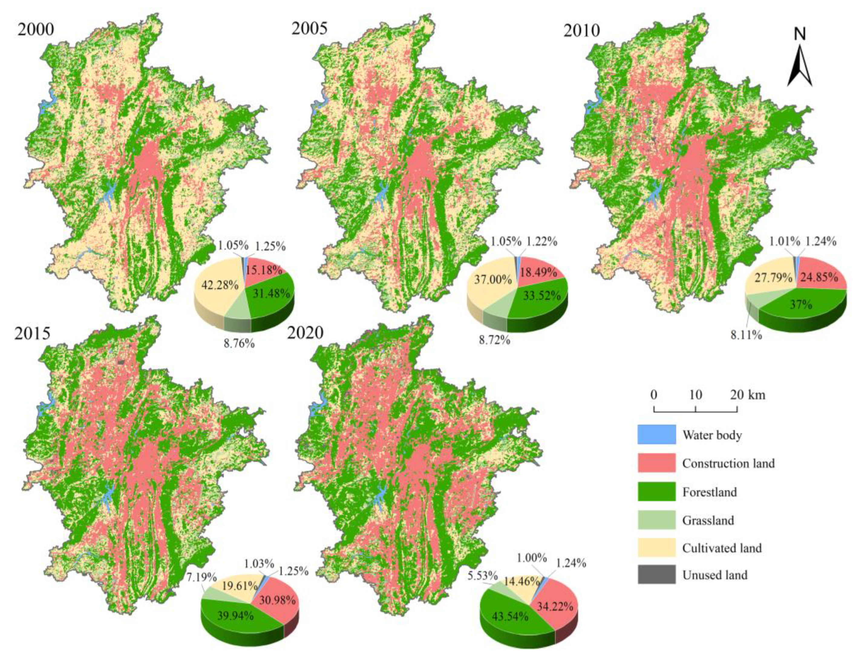
Cultivated land, forestland, and construction land were the most widespread landscape types, accounting for around 90% of the study area’s total area. As a result of the effects of increasing urbanization and environmental restoration efforts, the landscape types in CUAG changed dramatically from 2000 to 2020. These findings show that the area of construction land and forestland significantly increased by 224.26 km2 and 142.17 km2 respectively, whereas the area of cultivated land continuously decreased by 327.73 km2 during the study periods (Figure 2).
The area transfer matrix of landscape types in different periods shown the direction and degree of changes among different landscape types (Figure 3). This indicated that the transfer of landscape types in CUAG mainly concentrated on forestland, construction land, and cultivated land with the trend of the “transfer-out” for cultivated land and the “transfer-in” for forestland and construction land. However, the degree of transfer varied in different periods. From 2000 to 2015, the cultivated land was mainly transferred to construction land with an area of 296.13 km2, accounting for 86.4% of the total “transfer-out” area of cultivated land in the past 20 years. Since 2015, the rate of cultivated land transfer to construction land was slowed, whereas the area of cultivated land transfer to forestland increased significantly with the area of 196.60 km2.

3.2. Landscape Pattern Changes from 2000 to 2020

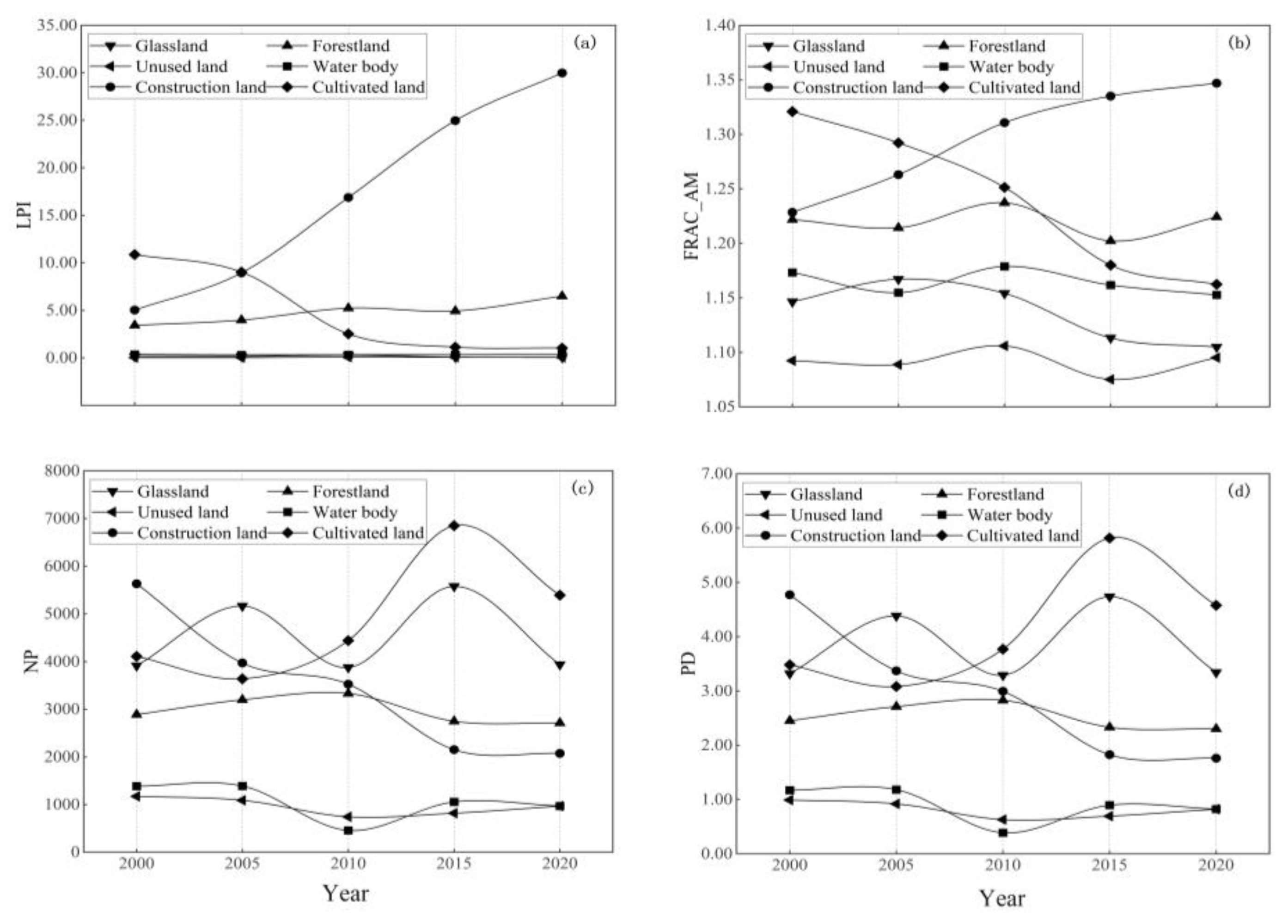
Figure 4 shows the changes in landscape metrics for three dominant landscape types at class level from 2000 to 2020. It was found that the LPI and FRAC_AM indices of construction land increased steadily, whereas the NP and PD indices of construction land decreased notably; however, the opposite patterns were displayed for cultivated land. This indicated that construction land patches tended to concentrated distribution with the patch fragmentation reduced, but the patch shape was more complex. On the contrary, due to the dramatic decrement of cultivated land during the study periods, the patch distribution of cultivated land was more fragmented and dispersed with its patch shape regularization. In addition, the changes of LPI, NP, and PD indices for forestland were similar to that for construction land; however, the variation of these indices was lower than that of construction land; the FRAC_AM index for forestland was fluctuated and remained relatively stable level from 2000 to 2020; this demonstrated that the degree of fragmentation and heterogeneity for forestland patches also decreased.
At the landscape level, the landscape pattern in CUAG also fluctuated significantly (Figure 5). The values of AI and CONTAG indices dropped from 86.03 and 47.65 in 2000 to 85.74 and 46.46 in 2005, respectively; and then, these two indices increased continuously from 2005 to 2020. These findings indicated that the landscape lumpiness, aggregation, and connectivity in CUAG were enhanced with the trend of a concentrated distribution during the study period (Figure 5a). However, the values of SHDI and SHEI indices increased significantly from 2000 to 2010, which was the period of frequent changes of landscape types in CUAG, changes that led to an upward trend of landscape heterogeneity and diversity level. From 2010 to 2020, with the rapid urbanization and the implementation of ecological restoration measures, construction land and forestland gradually became the dominant landscape types in CUAG, and the values of SHDI and SHEI indices were declined with the trend of landscape diversity decrement and landscape homogenization enhancement (Figure 5b).

3.3. Driving Factors of Landscape Pattern Changes

3.3.1. Temporal Driving Forces

Table 3 shows the fitting models of temporal driving factors for three dominated landscape types (cultivated land, forestland, and construction land) changes in CUAG. The model-fitting results were reasonable with the determination coefficient of these models greater than 0.94 (p < 0.05). These indicated that industrial structure was the dominant temporal driving factor of the three dominated landscape type changes in the study area. Ratio of tertiary industry structure (x11) had a negative driving effect for cultivated land changes and had a positive driving effect on the changes in forestland and construction land. In addition, population density (x7) and the ratio of primary industrial structure (x9) had a negative driving effect on cultivated land and construction land, respectively.

3.3.2. Spatial Driving Forces

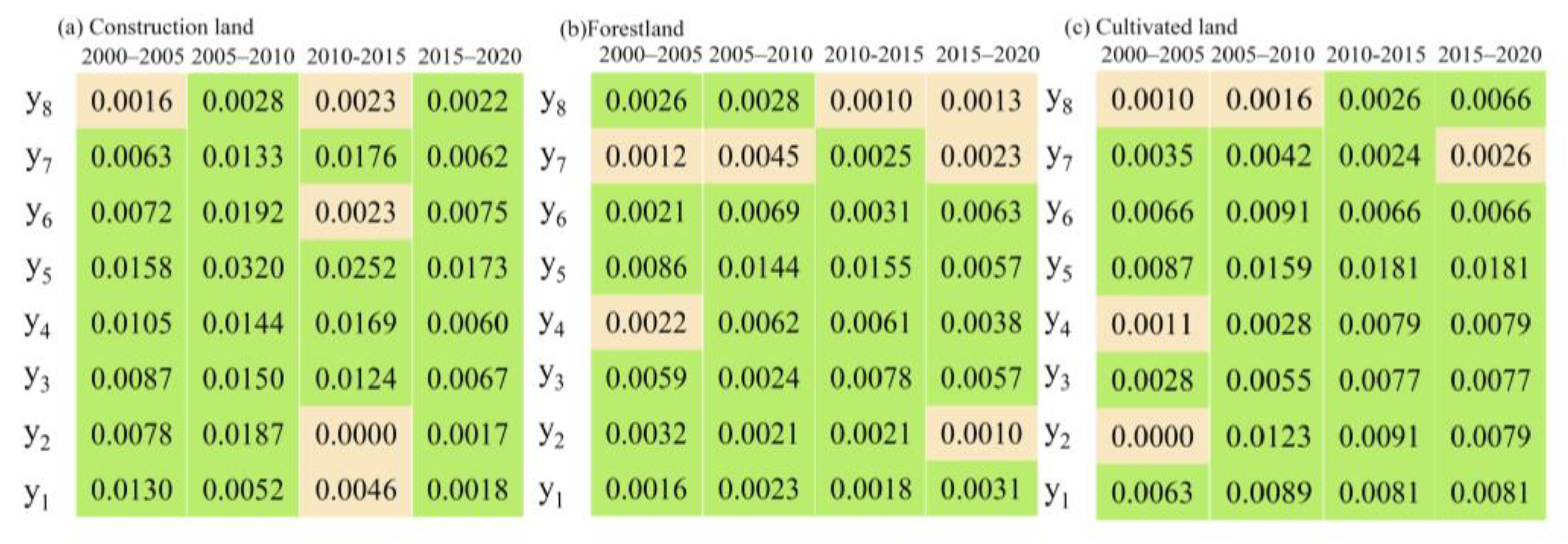
Figure 6 displayed the attribution analysis of different factors for the spatial evolution of three dominated landscape types in different periods by using the factor detection model. The dominant spatial driving factors of each landscape type in different periods were varied. Slope (y3), topographical relief (y5), elevation (y4), and distance to railway (y7) had significant effects on the spatial changes of construction land (p < 0.05), whereas GDP (y1), slope (y3), topographical relief (y5), and distance to railway (y6) had significant effects on the spatial changes of cultivated land and forest land (p < 0.05). On the whole, the explanatory power of physical factors (i.e., topographical relief (y5), elevation (y4), and slope (y3)) on spatial change of landscape pattern were stronger than that of socioeconomic factors and accessibility factors, with the q values of physical factors 1.11–22.28 times of other factors.
The interaction effects of various factors presented a synergistic relationship between nonlinear enhancement or two-factor enhancement (Figure 7). It was found that the interactive two factors could enhance the explanatory power of the factors affecting landscape pattern changes. The interaction of topographic relief (y5) with distance from railway (y7), elevation (y4), and slope (y3) had a strong explanatory power to the spatial change of the three dominant landscape types during the study period. This demonstrated that the coupling effect of natural condition and spatial accessibility were the dominant spatial driving factors of landscape pattern changes in the study area. In addition, the interaction of GDP (y1) or population density (y2) with natural factors (i.e., slope (y3), elevation (y4), and/or topographical relief (y5) had a relatively higher explanatory power in some periods.

4. Discussion

4.1. Landscape Pattern Dynamics of Karst Mountainous Cities

Research has previously shown that urbanization can lead to changes in landscape types and landscape patterns [54,55]. The ecological sensitivity of karst region in China is high, and the landscape pattern changes are particularly dramatic [56,57]. Urbanization expansion has been the dominant trend and direction of land use structure change in recent years as a result of economic growth, rising population, and social development, which has had a significant impact on the landscape pattern [58,59,60].
In this study, the landscape pattern in CUAG saw a series of changes from 2000 to 2020 as a result of growing urbanization, with a tendency of clearly increasing building land and dramatically decreasing cultivated land, according to this study. This finding is in line with findings from other studies [36,60]. This illustrates that the main kind of landscape pattern change during urbanization is the conversion of cultivated land to construction land. In addition, the encroachment of ecological land (such as forestland and grassland) during the expansion of construction land is also one of the characteristics of landscape change in the process of urbanization (Figure 3). Wu [9] and Weng et al. [13] found that, with urban expansion, landscape pattern changes showed that ecological land (i.e., forestland, grassland, water body) was transformed into construction land. Furthermore, forestland was the dominant landscape type in CUAG, and the area of forestland increased steadily during the study periods (Figure 2 and Figure 4). This finding is consistent with the results of the study by Wang et al. [56] in Guiyang City. This is mainly benefited by the unique landscape matrix of karst mountainous cities. As a typical karst mountainous city, CUAG is characterized by large mountains stretching in patches and small hills sporadically distributed, and the land for construction is developed near the mountains, forming a unique urban–mountain mosaic landscape [54,56]. As a result, rich natural and near-natural forests depend on the mountains. On the other hand, the national and provincial ecological protection policies are also an important reason for the increasing area of forested land. For example, the Chinese government launched ecological restoration projects such as the Natural Forest Protection Program in 1998 and the Reforestation Program in 1999 [57], and the Guiyang city government has planned and built a mountain-river-wetland ecological network system mainly in urban mountains since 2000; and by 2020, the forest coverage rate of Guiyang city will reach 55% and the per capita park green space in the built-up area will be 13.2 km2 [58].
Landscape patterns in rapidly urbanizing areas have presented a remarkable, highly fragmented feature. The single, continuous natural patches have become complex, heterogeneous, and discontinuous mosaics [60,61,62]. In this study, along with the construction land in CUAG expanded extensively, its patch displayed a trend of concentrated distribution with the low fragmentation (Figure 2 and Figure 4). This finding is similar to the results of studies in the Mianzhu [63] and Saudi Arabian cities [64]. However, the patch shape in CUAG became more complex (Figure 2 and Figure 4). Unlike plains cities, construction land continuously shifted outward to form a central area. The number of patches and shape complexity were declining, indicating that construction land was gradually converging in number and regular in shape; on the one hand, this may be related to the expressways construction and relocation of industrial areas [64]; on the other hand, Guiyang City had gradually strengthened its urban spatial form control measures. Nevertheless, the expansion of construction land was limited by topographic factors such as elevation and slope, and the shape of construction land patches was more complex in mountainous areas [65,66]. However, the growth of construction land in the study area experienced two stages rapid expansion from 2000 to 2015 and slow expansion from 2015 to 2020. It might be influenced by urban planning and land use policy. During 2000–2015, the urbanization pattern of multi-group development in Guiyang City has driven the intense expansion of construction land. The urbanization rate rose from 25% to 52% [67]. The disorderly spreading of construction land posed a serious threat to sustainable urban development, intensified ecological fragmentation, and overloaded resource and environmental capacity. In order to promote compact urban patterns and control urban scale, local governments have implemented policies to strictly limit the growth of construction land. In particular, after 2015, the Guiyang city government proposed layout optimization land remediation measures, and these policies led to a slowdown in the growth rate of construction land in the study area from 2015 to 2020.
During 2010–2020, landscape tended to be monolithic, with a more concentrated distribution of the phenomenon, showing the phenomenon of landscape homogenization, which is consistent with the findings of previous studies [26,52,68]. With regard to the impact of land-use change on the structure of the landscape as construction land and woodlands develop into more complex landscapes and as their spatial organization become more disorganized, urban planning may be used to rationally optimize the ecology of the surrounding region. Second, we see that homogeneity is a crucial process that goes hand in hand with the spatial urbanization process. The landscape had gradually closed due to the growth of the forest, and is now less functionally designed and more simply laid out. Landscape uniformity was also being fueled at the same time by the abandonment of farming, urbanization, and infrastructural developments [26]. Therefore, how to fairly distribute landscape types and spatial distribution in the course of urbanization may be a trend for future land use landscape planning and environmental decision-making.

4.2. Driving Force of Landscape Pattern Dynamics

The research of spatial-temporal drivers of urban landscape change is the foundation for revealing the inner mechanism of landscape pattern-process-function, and also guarantees the optimization of landscape space and the construction of landscape ecological security pattern [31]. In this study, the ratio of tertiary industry structure and the ratio of primary industrial structure were the significantly exploratory temporal factors for landscape pattern changes in CUAG. These findings indicate that industrial structure was a key determinant of landscape pattern. These findings are consistent with previous related studies elsewhere that have shown the upgrading and adjustment of industrial structure as driver of urban expansion [48,69]. It is argued that economic structural transformation could accelerate urban expansion, since this process increased land demand associated with the growing private and foreign enterprises [69,70] and cities have competed intensively to attract economic development through improving infrastructure and setting up development zones [71,72]. Moreover, the demographic variables, total population, and population density are recognized to be positive independent factors of landscape pattern change [71,73,74,75]. This result also agrees with our study that population density is an essential determinant of landscape pattern. It makes intuitive sense that more space will be occupied as more people inhabit [71,76]. An increase in population density will inevitably give rise to higher demand on residence, public facilities, and transportation, which would accelerate landscape pattern change [71,77].
Among the spatial variables, natural factors and accessibility factors are frequently found to be exploratory factors of landscape pattern change during urban expansion [26,77]. Areas with low-lying terrain and flat topography are conducive to the formation of construction land [78,79,80]. It is argued that human activities will encounter fewer obstacles in areas with such topological characteristics [75]. In this study, topographic relief was considered the special factor in the spatial evolution of urban landscape patterns. Areas with large topographic relief have less human interference, and forests have significant advantages under this terrain [77,81]. Our results support such arguments. In addition, as for the accessibility factor, when the expansion of rapid urbanization slows down and the urban landscape develops in an aggregated manner, with the reorganization of the landscape as the main way, socio-economic factors and urban spatial accessibility gradually become the main factors affecting the spatial evolution of the landscape pattern, which corroborates the study of Sebastian [77]. In addition, high spatial accessibility brings about high land use intensity and expands urban space, the connection between districts is closer, towns are developed in succession. The construction of roads, highways, and railways organically connects distant towns. This promotes urbanization and changes the urban landscape pattern [71].
In this study, small cities, slow development, and a wealth of natural resources put the CUAG’s geographic location in terms of economics and transportation at a major disadvantage. The local ecological and cultural environment will suffer from overdevelopment and city-scale expansion. In order to create a city with ecological functions while combining its unique geographic endowment, it is vital to strike a balance between ecological environmental conservation and urbanization expansion.

5. Conclusions

We conclude the following: (1) the landscape structure in CUAG from 2000 to 2020 was drastically changed. The area of forestland and construction land continuously increased and became the dominant landscape types since 2015. The decrease of cultivated land is the main contribution of landscape structure change to a trend of rapid urbanization and ecologization. (2) The patch aggregation of construction land and forestland tended to improve, with the degree of fragmentation decreased and the patch shape complicated. Meanwhile, the patch fragmentation of cultivated land was intensified. During the study periods, urban landscape connectivity was improved; however, the trend of landscape homogenization was obvious with the level of landscape diversity declined. (3) Industrial structure was the dominant temporal influencing factor for major landscape types changes, topographic relief and the interaction factors between topographic relief and regional spatial accessibility or social economy were the main spatial influencing factors for landscape pattern changes. The findings of this study on the temporal and spatial changes of landscape patterns and their driving factors in typical karst mountainous cities could provide a reference for landscape pattern planning and the research of the relationship between landscape patterns and processes under the background of rapid urbanization and ecologization in mountainous regions.

Author Contributions

Conceptualization, Z.W. and Y.L.; methodology, Y.L.; software, X.Z., C.H. and J.L. validation, X.Z., C.H. and J.L.; formal analysis, Y.L.; investigation, X.Z.; resources, C.H.; data curation, Y.L.; writing—original draft preparation, Y.L.; writing—review and editing, Z.W.; visualization, Y.L.; supervision, Y.L.; project administration, Z.W.; funding acquisition, Z.W. All authors have read and agreed to the published version of the manuscript.

Funding

This research was funded by the National Nature Science Foundation of China (NSFC) project, grant number 42061039 and 41701319; and the Construction Program of Biology First-class Discipline in Guizhou, grant number GNYL (2017)009.

Institutional Review Board Statement

Not applicable.

Informed Consent Statement

Not applicable.

Data Availability Statement

Not applicable.

Conflicts of Interest

The authors declare no conflict of interest.

References

  1. Cushman, S.A.; McGariyal, K.; Neel, M.C. Parsimony in landscape metrics: Strength, universality, and consistency. Ecol. Indic. 2008, 8, 691–703. [Google Scholar] [CrossRef]
  2. Wang, L.; Wang, S.; Zhou, Y.; Zhu, J.; Zhang, J.; Hou, Y.; Liu, W. Landscape pattern variation, protection measures, and land use/land cover changes in drinking water source protection areas: A case study in Danjiangkou Reservoir, China. Glob. Ecol. Conserv. 2020, 21, e00827. [Google Scholar] [CrossRef]
  3. Wu, J. Effects of changing scale on landscape pattern analysis: Scaling relations. Landsc. Ecol. 2004, 19, 125–138. [Google Scholar] [CrossRef]
  4. Li, J.; Zhou, K.; Dong, H.; Xie, B. Cultivated land change, driving forces and its impact on landscape pattern changes in the Dongting Lake Basin. Int. J. Environ. Res. Public Health 2020, 17, 7988. [Google Scholar] [CrossRef]
  5. Liu, S.; Qing, Y.; Chen, W. Spatial-temporal dynamic analysis of land use and landscape pattern in Guangzhou, China: Exploring the driving forces from an urban sustainability perspective. Sustainability 2019, 11, 6675. [Google Scholar] [CrossRef] [Green Version]
  6. Tang, J.; Li, Y.; Cui, S.; Xu, L.; Ding, S.; Nie, W. Linking land-use change, landscape patterns, and ecosystem services in a coastal watershed of southeastern China. Glob. Ecol. Conserv. 2020, 23, e01177. [Google Scholar] [CrossRef]
  7. Bai, X.; Shi, P.; Liu, Y. Society: Realizing China’s urban dream. Nature 2014, 509, 158–160. [Google Scholar] [CrossRef] [Green Version]
  8. Grimm, N.B.; Faeth, S.H.; Golubiewski, N.E.; Redman, C.L.; Wu, J.; Bai, X.; Briggs, J.M. Global change and the ecology of cities. Science 2008, 319, 756–760. [Google Scholar] [CrossRef] [Green Version]
  9. Wu, J.; Li, X.; Luo, Y.; Zhang, D. Spatiotemporal effects of urban sprawl on habitat quality in the Pearl River Delta from 1990 to 2018. Sci. Rep. 2021, 11, 13981. [Google Scholar] [CrossRef]
  10. Liu, J.; Zhan, J.; Deng, X. Spatio-temporal patterns and driving forces of urban land expansion in China during the Economic Reform Era. AMBIO J. Hum. Environ. 2005, 34, 450–455. [Google Scholar] [CrossRef]
  11. Zhang, Z.; Su, S.; Xiao, R.; Jiang, D.; Wu, J. Identifying determinants of urban growth from a multi-scale perspective: A case study of the urban agglomeration around Hangzhou Bay, China. Appl. Geogr. 2013, 45, 193–202. [Google Scholar] [CrossRef]
  12. Olivia, S.; Boe-Gibson, G.; Stitchbury, G.; Brabyn, L.; Gibson, J. Urban land expansion in Indonesia 1992–2012: Evidence from satellite-detected luminosity. Aust. J. Agric. Resour. Ec. 2018, 62, 438–456. [Google Scholar] [CrossRef]
  13. Weng, Y. Spatiotemporal changes of landscape pattern in response to urbanization. Landsc. Urban Plan. 2007, 81, 341–353. [Google Scholar] [CrossRef]
  14. Kassouri, Y. Monitoring the spatial spillover effects of urbanization on water, built-up land and ecological footprints in sub-Saharan Africa. J. Environ. Manag. 2021, 300, 113690. [Google Scholar] [CrossRef] [PubMed]
  15. Rimal, B.; Zhang, L.; Stor, N.; Sloan, S.; Rijal, S. Urban Expansion Occurred at the Expense of Agricultural Lands in the Tarai Region of Nepal from 1989 to 2016. Sustainability 2018, 10, 1341. [Google Scholar] [CrossRef] [Green Version]
  16. Gretchen, C. Paradise lost? The ecological economics of biodiversity. Trends Ecol. Evol. 1995, 10, 257–258. [Google Scholar]
  17. Harvey, A. Nature’s services: Societal dependence on natural ecosystems. Corp. Environ. Strategy 1997, 6, 219. [Google Scholar]
  18. Li, J.; Zhou, K.; Xie, B.; Xiao, J. Impact of landscape pattern change on water-related ecosystem services: Comprehensive analysis based on heterogeneity perspective. Ecol. Indic. 2020, 133, 108372. [Google Scholar] [CrossRef]
  19. Fons, V.; Eric, A.; Markus, F.; Alt, F.; Arndt, H.; Binkenstein, J.; Blaser, S.; Blüthgen, N.; Böhm, S.; Hölzel, N.; et al. Towards the development of general rules describing landscape heterogeneity-multifunctionality relationships. J. Appl. Ecol. 2018, 56, 160–178. [Google Scholar]
  20. Liu, J.; Xu, Q.; Yi, J.; Huang, X. Analysis of the heterogeneity of urban expansion landscape patterns and driving factors based on a combined Multi-Order Adjacency Index and Geographic detector model. Ecol. Indic. 2022, 136, 108655. [Google Scholar] [CrossRef]
  21. Wu, J. The key research topics in landscape ecology. Acta Ecol. Sin. 2004, 24, 2074–2076. [Google Scholar]
  22. Estoque, R.; Murayama, Y. Landscape pattern and ecosystem service value changes: Implications for environmental sustainability planning for the rapidly urbanizing summer capital of the Philippines. Landsc. Urban Plan. 2013, 116, 60–72. [Google Scholar] [CrossRef]
  23. Dewan, A.M.; Yamaguchi, Y. Land use and land cover change in Greater Dhaka, Bangladesh: Using remote sensing to promote sustainable urbanization. Appl. Geogr. 2009, 29, 390–401. [Google Scholar] [CrossRef]
  24. Jiang, L.; Deng, X.; Seto, K.C. The impact of urban expansion on agricultural land use intensity in China. Land Use Policy 2013, 35, 33–39. [Google Scholar] [CrossRef]
  25. Xiao, J.; Shen, Y.; Ge, J.; Tateishi, R.; Tang, C.; Liang, Y.; Huang, Z. Evaluating urban expansion and land use change in Shijiazhuang, China, by using GIS and remote sensing. Landsc. Urban Plan 2006, 75, 69–80. [Google Scholar] [CrossRef]
  26. Jiménez-Olivencia, Y.; Ibáñez-Jiménez, Á.; Porcel-Rodríguez, L.; Zimmerer, K. Land use change dynamics in Euro-mediterranean mountain regions: Driving forces and consequences for the landscape. Land Use Policy 2021, 109, 105721. [Google Scholar] [CrossRef]
  27. Abhishek, N.; Jenamani, M.; Mahanty, B. Urban growth in Indian cities: Are the driving forces really changing? Habitat Int. 2017, 69, 48–57. [Google Scholar] [CrossRef]
  28. Li, J.; Liu, Y.; Yang, Y.; Liu, J. Spatial-temporal characteristics and driving factors of urban construction land in Beijing-Tianjin-Hebei region during 1985–2015. Geogr. Res. 2018, 37, 37–52. [Google Scholar]
  29. Lu, C.; Wu, Y.; Shen, Q.; Wang, H. Driving force of urban growth and regional planning: A case study of China’s Guangdong province. Habitat Int. 2013, 40, 35–41. [Google Scholar] [CrossRef]
  30. Getu, K.; Bhat, H.G. Analysis of spatio-temporal dynamics of urban sprawl and growth pattern using geospatial technologies and landscape metrics in Bahir Dar, Northwest Ethiopia. Land Use Policy 2021, 109, 105676. [Google Scholar] [CrossRef]
  31. Ji, J.; Wang, S.; Zhou, Y.; Liu, W.; Wang, L. Spatiotemporal change and landscape pattern variation of eco-environmental quality in Jing-Jin-Ji urban agglomeration from 2001 to 2015. IEEE Access 2020, 8, 125534–125548. [Google Scholar] [CrossRef]
  32. Wu, M.; Li, C.; Du, J.; He, P.; Zhong, S.; Wu, P.; Lu, H.; Fang, S. Quantifying the dynamics and driving forces of the coastal wetland landscape of the Yangtze River Estuary since the 1960s. Reg. Stud. Mar. Sci. 2019, 32, 100854. [Google Scholar] [CrossRef]
  33. Yang, Y.; Wang, K.; Liu, D.; Zhao, X.; Fan, J.; Li, J.; Zhai, X.; Zhang, C.; Zhan, R. Spatio-temporal variation characteristics of ecosystem service losses in the agro-pastoral ecotone of northern China. Int. J. Environ. Res. Public Health 2019, 16, 131138. [Google Scholar]
  34. Najafabadi, S.M.; Soffianian, A.; Rahdari, V.; Amiri, F.; Pradhan, B.; Tabatabaei, T. Geospatial modeling to identify the effects of anthropogenic processes on landscape pattern change and biodiversity. Arab. J. Geosci. 2014, 8, 1557–1569. [Google Scholar] [CrossRef]
  35. Peng, Y.; Mi, K.; Qing, F.; Xue, D. Identification of the main factors determining landscape metrics in semi-arid agro-pastoral ecotone. J. Arid Environ. 2016, 124, 249–256. [Google Scholar] [CrossRef]
  36. Gong, Y.; Li, J.; Li, Y. Spatio-temporal characteristics and driving mechanisms of arable land in the Beijing-Tianjin-Hebei region during 1990–2015. Socio-Econ. Plan. Sci. 2020, 70, 100720. [Google Scholar] [CrossRef]
  37. Tanovic, M.; Golijanin, J.; Unjar, S. Impact of population on the karst of east sarajevo (bosnia and herzegovina). J. Geogr. Inst. 2019, 69, 95–107. [Google Scholar] [CrossRef]
  38. Zhang, Y.; Xiong, K.; Yu, Y.; Xu, M.; Cheng, W.; Tan, D.J. Daily variations of soil respiration among three types of non-wood forest in karst rocky desertification areas, Southern China. Zhongnan Linye Keji Daxue Xuebao 2019, 39, 92–99. [Google Scholar]
  39. Fan, Z.; Li, J.; Yue, T.; Zhou, X.; Lan, A. Scenarios of land cover in karst area of Southwestern China. Environ. Earth Sci. 2015, 74, 6407–6420. [Google Scholar] [CrossRef]
  40. Gao, J.; Jiang, Y.; Anker, Y. Contribution analysis on spatial tradeoff/synergy of karst soil conservation and water retention for various geomorphological types: Geographical detector application. Ecol. Indic. 2021, 125, 107470. [Google Scholar] [CrossRef]
  41. Liao, S.; Cai, H.; Tian, P.; Zhang, B.; Li, Y. Combined impacts of the abnormal and urban heat island effect in Guiyang, a typical karst mountain city in China. Urban Clim. 2022, 41, 101014. [Google Scholar] [CrossRef]
  42. Li, H.; Dong, L.; Ren, J. Industrial symbiosis as a countermeasure for resource dependent city: A case study of Guiyang, China. J. Clean. Prod. 2015, 107, 252–266. [Google Scholar] [CrossRef]
  43. Zhang, Q.; Chen, C.; Wang, J.; Yang, D.; Zhang, Y.; Wang, Z.; Gao, M. The spatial granularity effect, changing landscape patterns, and suitable landscape metrics in the Three Gorges Reservoir area, 1995–2015. Ecol. Indic. 2020, 114, 106259. [Google Scholar] [CrossRef]
  44. Zhang, X.; Wang, G.; Xue, B.; Zhang, M.; Tan, Z. Dynamic landscapes and the driving forces in the Yellow River Delta wetland region in the past four decades. Sci. Total Environ. 2021, 787, 147644. [Google Scholar] [CrossRef] [PubMed]
  45. Zhang, Y.; Li, Y.; Gao, H.; Liu, H. Eco-service functions based on land transfer matrix: A case study of Xianlin, a new urban area in Nanjing. J. Ecol. Rural Environ. 2014, 30, 800–805. [Google Scholar]
  46. Liu, Y.; Heuvelink, G.B.; Bai, Z.; He, P.; Xu, X.; Ding, W.; Huang, S. Analysis of spatio-temporal variation of crop yield in china using stepwise multiple linear regression-sciencedirect. Field Crop Res. 2021, 264, 108098. [Google Scholar] [CrossRef]
  47. Wang, Y.; Duan, X.; Yang, Q.; Wang, L.; Zou, H. Spatial-temporal characteristics and driving factors of urban construction land in Jiangsu Province in the last 30 years. Changjiang Liuyu Ziyuan Yu Huanjing 2019, 28, 1531–1540. [Google Scholar]
  48. Deng, L.; Zhang, Q.; Cheng, Y.; Cao, Q.; Wang, Z.; Wu, Q.; Qiao, J. Underlying the influencing factors behind the heterogeneous change of urban landscape patterns since 1990: A multiple dimension analysis. Ecol. Indic. 2022, 140, 108967. [Google Scholar] [CrossRef]
  49. Du, J.; Chen, Z. Path analysis using SPSS linear regression method. Biol. Bull. 2010, 45, 4–6. [Google Scholar]
  50. Kinfu, S.; Wato, T.; Negash, T. Study on character association and path analysis in Korarima (Aframomum corrorima (Braun) Jansen) germplasms at Jimma Southwestern. Ethiop. Heliyon 2022, 8, e08812. [Google Scholar] [CrossRef]
  51. Hua, D.; Hao, X. Spatio-temporal change and drivers analysis of desertification in the arid region of northwest China based on geographic detector. Environ. Chall. 2021, 4, 100082. [Google Scholar]
  52. Wang, J.; Zhang, T.; Fu, B. A measure of spatial stratified heterogeneity. Ecol. Indic. 2016, 67, 250–256. [Google Scholar] [CrossRef]
  53. Wang, Y.; Wang, S.; Zhang, H.; Jin, L.; Su, Y.; Wu, K. Identifying the determinants of housing prices in China using spatial regression and the geographical detector technique. Appl. Geogr. 2017, 79, 26–36. [Google Scholar] [CrossRef]
  54. Chen, X.; Wang, Z.; Bao, Y. Cool island effects of urban remnant natural mountains for cooling communities: A case study of Guiyang, China. Sustain. Cities Soc. 2021, 71, 102983. [Google Scholar]
  55. Huang, M.; Li, Y.; Xia, C.; Zeng, C.; Zhang, B. Coupling responses of landscape pattern to human activity and their drivers in the hinterland of Three Gorges Reservoir Area. Glob. Ecol. Conserv. 2022, 33, e01992. [Google Scholar] [CrossRef]
  56. Wang, Z.; Liu, Y.; Li, Y.; Su, Y. Response of ecosystem health to land use changes and landscape patterns in the karst, ountainous regions of southwest China. Int. J. Environ. Res. Public Health 2022, 19, 3273. [Google Scholar]
  57. Qiu, S.; Zheng, H.; Meersmans, J. How can massive ecological restoration programs interplay with social-ecological systems? A review of research in the South China karst region. Sci. Total Environ. 2021, 807, 150723. [Google Scholar] [CrossRef]
  58. Zhu, G. Scientific Concept of Development Guidance of Ecological Civilization City Construction Research in Guiyang City as an Example. Master’s Thesis, University of Wuhan, Wuhan, China, 2014. [Google Scholar]
  59. Zhang, M.; Wang, K.; Liu, H.; Zhang, C. Responses of spatial-temporal variation of Karst ecosystem service values to landscape pattern in northwest of Guangxi, China. Chin. Geogr. Sci. 2011, 21, 446–453. [Google Scholar] [CrossRef]
  60. Hyandye, C.; Martz, L.W. A Markovian and cellular automata land-use change predictive model of the Usangu Catchment. Int. J. Remote Sens. 2017, 38, 64–81. [Google Scholar] [CrossRef]
  61. Scanlon, B.R.; Reedy, R.C.; Stonestrom, D.A.; Prudic, D.E.; Dennehy, K.F. Impact of land use and land cover change on groundwater recharge and quality in the southwestern US. GCB Bioenergy 2005, 11, 1577–1593. [Google Scholar] [CrossRef]
  62. Dadashpoor, H.; Azizi, P.; Moghadasi, M. Land use change, urbanization, and change in landscape pattern in a metropolitan area. Sci. Total Environ. 2019, 655, 707–719. [Google Scholar] [CrossRef] [PubMed]
  63. Fu, F.; Deng, S.; Wu, D.; Liu, W.; Bai, Z. Research on the spatiotemporal evolution of land use landscape pattern in a county area based on CA-Markov model. Sustain. Cities Soc. 2022, 80, 103760. [Google Scholar] [CrossRef]
  64. Alqurashi, A.F.; Kumar, L. Spatiotemporal patterns of urban change and associated environmental impacts in five Saudi Arabian cities: A case study using remote sensing data. Habitat Int. 2016, 58, 75–88. [Google Scholar] [CrossRef]
  65. Xiao, R.; Cao, W.; Liu, Y.; Lu, B. The impacts of landscape patterns spatio-temporal changes on land surface temperature from a multi-scale perspective: A case study of the Yangtze River Delta. Sci. Total Environ. 2022, 821, 153381. [Google Scholar] [CrossRef]
  66. Macdonald, D.; Crabtree, J.R.; Wiesinger, G.; Dax, T.; Stamou, N.; Fleury, P.; Lazpita, J.G.; Gibon, A. Agricultural abandonment in mountain areas of Europe: Environmental consequences and policy response. J. Environ. Manag. 2000, 59, 47–69. [Google Scholar] [CrossRef]
  67. Yan, W. Study on the Water Quality Response and Health Management of the Nanming River in the Process of Urbanization in Guiyang City. Master’s Thesis, North China University of Water Resources and Electric Power, Zhengzhou, China, 2017. [Google Scholar]
  68. Bruegmann, R. Sprawl: A Compact History; University of Chicago Press: Chicago, IL, USA, 2005. [Google Scholar]
  69. Jiang, S.; Meng, J.; Zhu, L.; Cheng, H. Spatial-temporal pattern of land use conflict in China and its multilevel driving mechanisms. Sci. Total Environ. 2021, 801, 149697. [Google Scholar] [CrossRef]
  70. Zhang, Q.; Su, S. Determinants of urban expansion and their relative importance: A comparative analysis of 30 major metropolitans in China. Habitat Int. 2016, 58, 89–107. [Google Scholar] [CrossRef]
  71. Huang, Z.; Wei, Y.; He, C.; Li, H. Urban land expansion under economic transition in China: A multi-level modeling analysis. Habitat Int. 2015, 47, 69–82. [Google Scholar] [CrossRef]
  72. Angel, S.; Parent, J.; Civco, D.L.; Blei, A.; Potere, D. The dimensions of global urban expansion: Estimates and projections for all countries, 2000–2050. Prog. Plan. 2011, 75, 53–107. [Google Scholar] [CrossRef]
  73. Maimaitijiang, M.; Ghulam, A.; Sandoval, J.; Maimaitiyiming, M. Drivers of land cover and land use changes in St. Louis metropolitan area over the past 40 years characterized by remote sensing and census population data. Int. J. Appl. Earth Obs. 2015, 35, 161–174. [Google Scholar] [CrossRef]
  74. Su, S.; Jiang, Z.; Qi, Z.; Zhang, Y. Transformation of agricultural landscapes under rapid urbanization: A threat to sustainability in Hang-Jia-Hu region, China. Appl. Geogr. 2011, 31, 439–449. [Google Scholar] [CrossRef]
  75. Long, H.; Liu, Y.; Wu, X.; Dong, G. Spatio-temporal dynamic patterns of farmland and rural settlements in Su-Xi-Chang region: Implications for building a new countryside in coastal China. Land Use Policy 2009, 26, 322–333. [Google Scholar] [CrossRef]
  76. Peng, W.; Wang, G.; Zhou, J.; Zhao, J.; Yang, C. Studies on the temporal and spatial variations of urban expansion in Chengdu, western China, from 1978 to 2010. Sustain. Cities Soc. 2015, 17, 141–150. [Google Scholar] [CrossRef] [Green Version]
  77. Sebastian, E.; Kerstin, P. Landscape changes in Norwegian mountains: Increased and decreased accessibility, and their driving forces. Land Use Policy 2016, 54, 235–245. [Google Scholar]
  78. Li, J.; Cheng, L.; Zhu, F.; Song, C.; Wu, J. Spatiotemporal pattern of urbanization in Shanghai, China between 1989 and 2005. Landsc. Ecol. 2013, 28, 1545–1565. [Google Scholar] [CrossRef]
  79. Tan, R.; Liu, Y.; Liu, Y.; He, Q.; Ming, L.; Tang, S. Urban growth and its determinants across the Wuhan urban agglomeration, central China. Habitat Int. 2014, 44, 268–281. [Google Scholar] [CrossRef]
  80. Li, X.; Zhou, W.; Ouyang, Z. Forty years of urban expansion in Beijing: What is the relative importance of physical, socioeconomic, and neighborhood factors? Appl. Geogr. 2013, 38, 1–10. [Google Scholar] [CrossRef]
  81. Cartier, C. ‘Zone fever’, the arable land debate, and real estate speculation: China’s evolving land use regime and its geographical contradictions. J. Contemp. China 2001, 10, 445–469. [Google Scholar] [CrossRef]
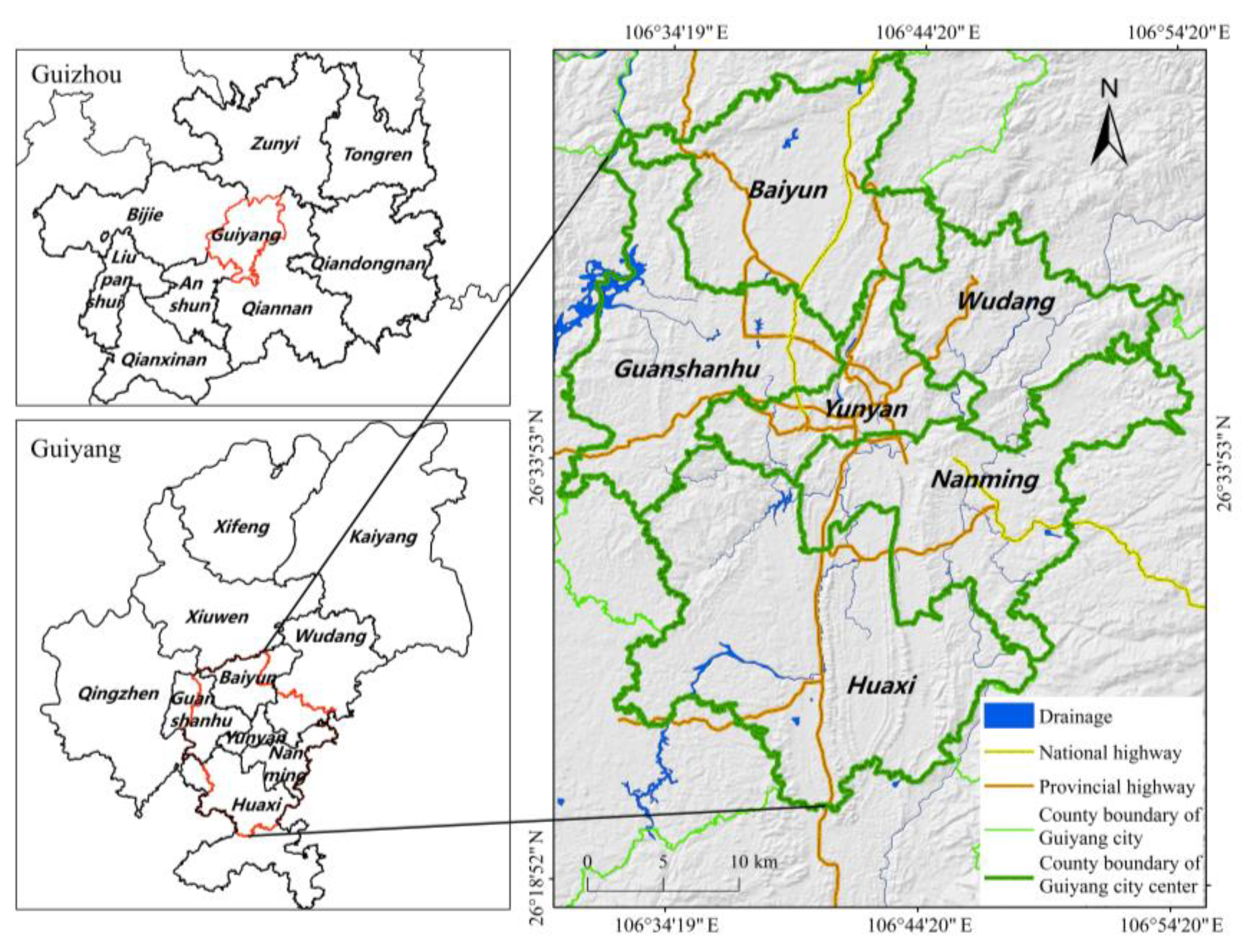
Figure 1. Location of study area.
Sustainability 14 08274 g001
Figure 2. The spatial pattern of the land use in the central urban area of Guiyang City (CUAG) from 2000 to 2020.
Sustainability 14 08274 g002
Figure 3. Transfer direction between the different landscape types in CUAG from 2000 to 2020.
Sustainability 14 08274 g003
Figure 4. Changes in the landscape pattern index of CUAG from 2000 to 2020 at class level. (a) LPI, Largest patch index; (b) FRAC_AM, Area-weighted mean fractal dimension index; (c) NP, Number of patches; (d) PD, Patch density.
Sustainability 14 08274 g004
Figure 5. Changes in the landscape pattern index of CUAG from 2000 to 2020 at landscape level they should be listed as: (a) AI and CONTAG index of CUAG; (b) SHDI and SHEI index of CUAG.
Sustainability 14 08274 g005
Figure 6. Map of drivers of the spatial landscape change based on geographic detector. (a) Construction land factors detection, (b) forest factors detection, (c) cultivated land factors detection: y1~y8 represent GDP, population density, slope, altitude, topographical relief, distance to railway, distance to expressway, distance to water system in turn. The green rectangle indicates that the driving result is significant at the 95% confidence level; yellow rectangular indicates that the driving result is not significant.
Sustainability 14 08274 g006
Figure 7. Interaction detection between the factors leading to major landscape types changes from 2000 to 2020: y1~y8 represent GDP, population density, slope, altitude, topographical relief, distance to railway, distance to high speed, distance to water system in turn.
Sustainability 14 08274 g007
Table 1. Driving Factors of Landscape Pattern in CUAG.
Temporal Driving Factors
DimensionNameDescription
Economic levelGDP (x1)Gross Domestic Product, it is the result of the productive activity of all resident units in a country (or region) during a certain period of time.
Per capita GDP (x2)The ratio of the GDP of a region to the resident population of the region during the accounting period.
Indices of gross domestic product (x3)It is a relative number that reflects the trend and extent of changes in GDP over a certain period of time.
Total investment in fixed assets (x4)It is the workload of construction and acquisition activities of fixed assets expressed in monetary terms.
Total retail sales of consumer goods (x5)Refers to the amount of physical goods sold by enterprises (units) to individuals and social groups through transactions, not for production or business use, and the amount of revenue earned from the provision of food and beverage services.
Local financial revenue (x6)Consists of the region’s fiscal revenues. Local fiscal revenues include local budget revenues and extra-budgetary revenues.
Population sizePopulation density (x7)Number of people per unit of land area.
Natural population growth rate (x8)Ratio of natural increase in population in a given period to the average total population in the same period.
Industrial structureRatio of primary industrial structure (x9)Value added and employment in the primary industrial as a share of GDP and total labor force.
Ratio of secondary industry structure (x10)Value added and employment in the secondary industry as a share of GDP and total labor force.
Ratio of tertiary industry structure (x11)Value added and employment in the tertiary industry as a share of GDP and total labor force.
Spatial Driving Factors
DimensionNameDescription
Socioeconomic factorsGDP (y1)Kilometer grid data to measure the level of economic development of a region.
Population density (y2)Kilometer grid data, indicating the population density of the area.
Natural factorsSlope (y3)The degree of steepness of the surface unit, the ratio of the vertical height of the slope to the distance in the horizontal direction.
Elevation (y4)The vertical distance above sea level at a point on the ground.
Topographical relief (y5)The difference between the elevation of the highest point and the elevation of the lowest point in a particular area.
Accessibility factorsDistance to river (y6)Distance between urban construction land and river.
Distance to railway (y7)Distance between urban construction land and railway.
Distance to highway (y8)Distance between urban construction land and highway.
Table 2. Description of landscape pattern index.
LevelNameAcronymDescription
CPatch densityPDThe proportion of the landscape area to the number of patches of the same patch type
Largest patch indexLPIThe area occupied by the largest patch of each class as a percentage of the overall area
Number of patchesNPThe heterogeneity and fragmentation of landscape
Area-weighted mean
fractal dimension index
FRAC_AMThe complexity and stability of landscape type shape
LAggregation indexAIA metric for the degree of spatial pattern aggregation
ContagionCONTAGWhen all patch types are considered, the measure can reflect the spatial distribution features and mixing state of all patch types at the same time
Shannon’s diversity indexSHDIRelative patch diversity within a range of 0–1
Shannon’s evenness indexSHEIRelative patch evenness within a range of 0–1
Table 3. Regression result of the influence factors of landscape pattern evolution.
Landscape TypeEquation of RegressionDriving FactorsDetermination CoefficientResidual Path Coefficient
Cultivated land y = 182.809 0.573 x 11 0.996 x 7 Population density (−)
Ratio of tertiary industry structure (−)
0.9980.045
Forestland y = 72.991 + 0.260 x 11 Ratio of tertiary industry structure (+)0.9430.239
Construction land y = 80.234 + 0.308 x 11 0.332 x 9 Ratio of tertiary industry structure (+)
Ratio of primary industrial structure (−)
0.9990.032
Publisher’s Note: MDPI stays neutral with regard to jurisdictional claims in published maps and institutional affiliations.