A Strategy for System Risk Mitigation Using FACTS Devices in a Wind Incorporated Competitive Power System

Abstract

Electricity demand is sharply increasing with the growing population of human beings. Due to financial, social, and political barriers, there are lots of difficulties when building new thermal power plants and transmission lines. To solve this problem, renewable energy sources and flexible AC transmission systems (FACTS) can operate together in a power network. Renewable energy sources can provide additional power to the grid, whereas FACTS devices can increase the thermal limit of existing transmission lines. It is always desirable for an electrical network to operate under stable and secure conditions. The system runs at risk if any abnormality occurs in the generation, transmission, or distribution sections. This paper outlines a strategy for reducing system risks via the optimal operation of wind farms and FACTS devices. Here, a thyristor-controlled series compensator (TCSC) and a unified power flow controller (UPFC) have both been considered for differing the thermal limit of transmission lines. The impact of the wind farm, as well as the combined effect of the wind farm and FACTS devices on system economy, were investigated in this work. Both regulated and deregulated environments have been chosen to verify the proposed approach. Value at risk (VaR) and cumulative value at risk (CVaR) calculations were used to evaluate the system risk. The work was performed on modified IEEE 14 bus and modified IEEE 30-bus systems. A comparative study was carried out using different optimization techniques, i.e., Artificial Gorilla Troops Optimizer Algorithm (AGTO), Honey Badger Algorithm (HBA), and Sequential Quadratic Programming (SQP) to check the effect of renewable integration in the regulated and deregulated power systems in terms of system risk and operating cost.

1. Introduction

A continuous decrease in coal and fossil fuel for power is forcing power generation companies to think about the alteration of thermal power. In this scenario, renewable energy can play a vital role in generating energy and constitute a primary or secondary energy source in the power network [1]. Due to the high efficiency of, and dependency on, nature, wind, and solar energy, these energy sources are considered the main sources of renewable energy [2].

Electricity demand is also rising every day due to the increase in human living standards throughout the world. On the other hand, the new construction of transmission channels also faces challenges due to economic, geographical, political, and social obstructions. Thus, it is a necessity to upsurge the flow limit of existing transmission lines to fulfil the increasing power demand. The line flow limit of a transmission line can be varied by the operation of FACTS devices.

Currently, power sectors are trying to move towards deregulated power systems instead of the existing regulated system. The conversion of the power system from regulated to deregulated provides an economic benefit to society. The large competition among all market players in the power sector provides a transparent system, benefiting energy customers. The incorporation of FACTS devices into renewable integrated competitive power systems is complex yet will provide the highest economic benefit to this type of system. In the recent past, several kinds of research have been carried out by different researchers.

Elmitwally and Eladl [3] proposed a way to work with an ideally distributed, multi-type FACTS controller system within a wind-incorporated power system. This paper aims to intensify the existing approximations of the extended span benefits. Paper [4] depicts the consequence of renewable integration in the deregulated power market, by the lower construction interruptions, and also volume cycles through simulation. A simple and optimal allocation process of TCSC and UPFC with wind generators has been described in [5] for improved economic profit in deregulated power systems. Nature-inspired optimization algorithms have become popular for solving different control and stability issues caused by increased renewable use [6]. These include frequency stability [7,8], cost optimization [9], energy management [10] and storage optimization [11,12]. Following this trend, reference [13] presents an adaptive artificial neural network-based modified particle swarm optimization (PSO) algorithm to optimize the real-time congestion control in a power system. Wu et al. [14] present a stochastic algorithm to find the optimal generator schedule and the required load response to minimize transmission overload risk. Bhattacharya and Kumar [15] developed a GSA-based improvement approach for the optimal distribution of FACTS devices in a transmission system. Kavitha and Neela [16] have contemplated the effect of the FACTS device arrangement for improving security under expanded system loading conditions. Packiasudha et al. [17] proposed a cumulative gravitational search algorithm (CGSA) for optimum positioning of FACTS devices in an unregulated energy environment, taking into account the goal of minimizing the transmission losses of the system. The authors of [18] described a GSA-based advancement strategy for the optimum coordination of multi-type FACTS with standing reactive power, existing in a connected power network. In [19], the authors assess the process of deregulation policies and their micro and macroeconomic effects on the energy sector, specifically on electricity, by reviewing the literature on the subject. Dawn et al. [20] presented a method for evaluating the wind speed uncertainty of a wind-integrated electricity system in a completely deregulated environment. In [21], the authors proposed an effective optimization technique to achieve maximum social welfare and profit by minimizing the adverse effect of imbalance cost. Chinmoy et al. [22] examined the various components of modeling wind energy systems for integration into deregulated power markets, including investment, policy, performance, and social benefits. The authors of [4] noted that, due to the introduction of deregulation, there are many speculations that cycles may form in generation capacity. Wang et al. [23] state that the multi-energy microgrid is a key factor in the electricity market due to the complementary and flexible operation of multi-energy. Paper [24] describes a bidding strategy for a grid-connected microgrid which has been devised to generate higher profits for the microgrid. In [25], the authors state that in global decarbonization, variable renewable electricity (VRE) plays an important role. For additional integration of the costs for both power systems and consumer intermittency, uncertainty, and the integration of variable renewable energy (VRE) are required. The authors of [26] state that wind production increases in the power market when considering optimal power-to-heat capacity. A district heating optimization model was developed by the authors using linear programming and a free programming language called Julia. Bashir et al. [27] depict the solar commitment problem that solar generators face if they adopt a partially deregulated solar system. This research shows the probabilistic approach for tackling this problem, in which they combine a solar performance model with weather measurement and forecast data. In [28], the authors note that markets involved in electricity are more complex and involve long lead times, including feedback, that are generally hard to interpret and are influenced by large political and environmental concerns and objectives.

In [29], the authors minimize the imbalance cost with the help of a Smart Flower Optimization Algorithm (SFOA) and Honey Badger Algorithm (HBA) for a wind and solar PV integrated power system. Here, imbalance arises due to the variations of predicted wind speed and actual wind speed of the system. In a wind farm integrated system, to minimize the system risk and to minimize the system generation cost, pumped hydro storage systems are optimally placed in the power system by using an artificial bee colony (ABC) algorithm and a moth flame optimization (MFO) algorithm [30].

Recently, profit allocation for a virtual power plant (VPP)-based electricity market model was introduced for several other objectives, such as fairness of profit allocation, the attraction of participating entities, and stability of cooperative alliance. To solve this, a market model, multi-objective evolutionary optimization algorithm is used by the authors of [31]. To encourage consumers, a real-time pricing (RTP) and demand response (DR) program are mathematically modelled and implemented to solve energy management problems via scheduling residential loads. To solve the energy management problem, a hybrid algorithm using an enhanced differential evolution (EDE) and a genetic algorithm (GA) were used by the authors of [32]. Luis Corona et al. [33] presented a model to build and identify the main drivers of price convergence in Central-Western Europe (CWE) after applying the complex flow-based market coupling (FBMC) mechanism based on publicly available data. To optimize social welfare, the FBMC mechanism is implemented in the CWE electricity market. To solve the strategic bidding problem in an electricity market, the AC optimal power flow (ACOPF) problem explores more opportunities than the DCOPF-based market clearing problem (for the market-clearing process) [34].

After the completion of a detailed literature review, it can be seen that various risk assessment and mitigation goals have been accomplished, yet some queries still remain, such as: (a) What will be the influence of the risk assessment process on the power system? (b) What will be the outcome of wind farm integration on system risk? (c) How can FACTS devices control the system risk in a wind incorporated deregulated system? (d) How do several optimization methods offer a better, risk-minimized system in an electrical network? all of which are discussed in this work.

The present work has been performed while considering the research gaps found in the literature. The key offerings of this work are:

• The importance of incorporating FACTS devices in a regulated and deregulated system was studied in terms of system economy, locational marginal pricing (LMP), and system voltage profile;
• The system risk was calculated by considering several abnormalities in the system (i.e., bus failure, line outage, system load increment, etc.). The worst condition was chosen based on the risk assessment parameter (i.e., VaR, CVaR) values;
• Placement of a wind farm within the system while checking the system risk;
• The optimal operation of FACTS devices was performed along with the wind farm while checking the system risk;
• Comparative studies of system risk and system economy were completed using three different optimization techniques, i.e., Artificial Gorilla Troops Optimizer Algorithm (AGTO), Honey Badger Algorithm (HBA), and Sequential Quadratic Programming (SQP);
• The artificial gorilla troops optimizer algorithm (AGTO) was utilized for the first time concerning this kind of risk mitigation problem, which constitutes the uniqueness of this paper.

2. System Modeling

This section displays the mathematical modeling of the FACTS devices along with social welfare, locational marginal pricing, and risk assessment parameters.

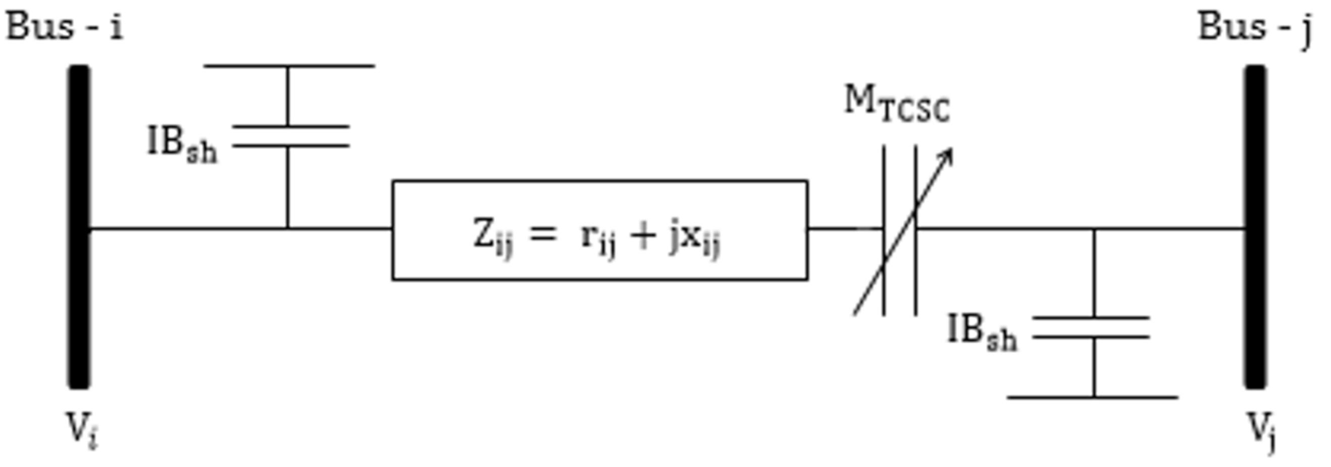
2.1. Thyristor Controlled Series Compensator (TCSC)

A TCSC includes a capacitor allied in series with an inductor and a brace of opposite-poled thyristors. The inductor reactance may be accustomed by varying the firing angle of the thyristors, which can alter the effective impedance of the TCSC [5]. The static model of TCSC has shown in Figure 1. The reactance of the line after TCSC placement (M_Line) is calculated as follows:

$${\mathrm{M}}_{\mathrm{Line}}={ \mathrm{M}}_{\mathrm{ij}}+{ \mathrm{M}}_{\mathrm{TCSC}}$$

(1)

$$\mathrm{Where} {\mathrm{M}}_{\mathrm{TCSC}}={ \mathrm{L}}_{\mathrm{TCSC}}\times { \mathrm{M}}_{\mathrm{Line}}$$

(2)

Here, M_ij is the line reactance before TCSC placement and M_TCSC is the reactance of the TCSC devices. The considered TCSC compensation level (L_TCSC) is as follows: $-0.7\le {\mathrm{L}}_{\mathrm{TCSC}}\le 0.2$. The TCSC’s reactance operating range has been set between $-0.7{\mathrm{M} }_{\mathrm{Line}}$ and $0.2{ \mathrm{M}}_{\mathrm{Line}}$.

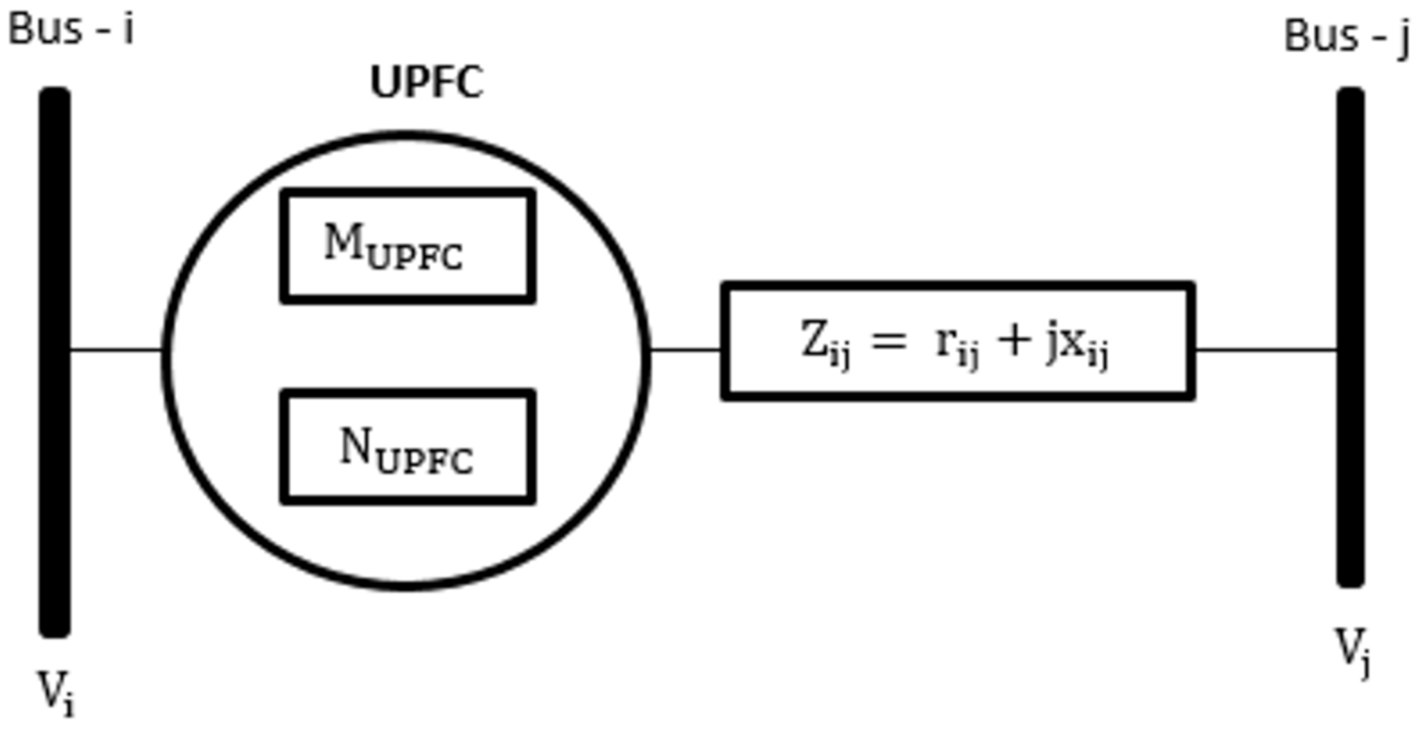
2.2. Unified Power Flow Controller (UPFC)

The UPFC may change the amplitude and phase angle of the series injected voltage as well as the reactive current drawn by the shunt connected voltage source converter, either concurrently or separately. UPFC is made up of two voltage source converters connected back-to-back through a DC connection [5]. Figure 2 depicts the UPFC static model. The reactance of UPFC (M_UPFC) is related to the reactance of the transmission line (M_ij) on which the UPFC is to be installed.

$${\mathrm{M}}_{\mathrm{Line}}={ \mathrm{M}}_{\mathrm{ij}}+{ \mathrm{M}}_{\mathrm{UPFC}}$$

(3)

$$\mathrm{Where} {\mathrm{M}}_{\mathrm{UPFC}}={ \mathrm{L}}_{\mathrm{UPFC}}\times { \mathrm{M}}_{\mathrm{Line}}$$

(4)

The considered operational range of UPFC’s compensation level (L_UPFC) is: $-0.7\le {\mathrm{L}}_{\mathrm{UPFC}}\le 0.2$. The working range of the UPFC’s series reactance (M_Line) has been set between $-0.7{ \mathrm{M}}_{\mathrm{Line}}$ and $0.2{ \mathrm{M}}_{\mathrm{Line}}$. ${\mathrm{N}}_{\mathrm{UPFC}}$ is the injected or extracted reactive power through the shunt converter. The operational range of ${\mathrm{N}}_{\mathrm{UPFC}}$ (MVAr) is taken into account in this study as follows:

$$-100\le {\mathrm{N}}_{\mathrm{UPFC}}\le 100$$

(5)

2.3. Investment Cost of TCSC & UPFC

The cost of FACTS devices is critical in the economic picture of a power system. Because FACTS devices are expensive, when a new TCSC or UPFC is installed, the price optimization analysis must be used to assess whether the device is price effective across several sites [5]. The investment price of TCSC and UPFC are as follows:

$${\mathrm{Price}}_{\mathrm{TCSC}}=0.0015{ \mathrm{AB}}_{\mathrm{FACTS}}^2-0.713{ \mathrm{AB}}_{\mathrm{FACTS}}+153.75 \$/\mathrm{kVar}$$

(6)

$${\mathrm{Price}}_{\mathrm{UPFC}}=0.0003{ \mathrm{AB}}_{\mathrm{FACTS}}^2-0.2691{ \mathrm{AB}}_{\mathrm{FACTS}}+188.22 \$/\mathrm{kVar}$$

(7)

$$\mathrm{Where} {\mathrm{AB}}_{\mathrm{FACTS}}=\left|{\mathrm{N}}_{\mathrm{A}}\right|-\left|{\mathrm{N}}_{\mathrm{B}}\right|$$

(8)

The total asset price of FACTS devices is computed as follows:

$${\mathrm{Asset} \mathrm{Price}}_{\mathrm{FACTS}}=\left({\mathrm{PRICE}}_{\mathrm{FACTS}}\times { \mathrm{AB}}_{\mathrm{FACTS}}\times 1000 \right) \$$$

(9)

The yearly and hourly asset price of FACTS devices are expressed as

$${\mathrm{Y} \mathrm{Asset} \mathrm{Price}}_{\mathrm{FACTS}}={ \mathrm{Asset} \mathrm{Price}}_{\mathrm{FACTS}} \frac{\mathrm{ef}{\left(1+\mathrm{ef}\right)}^{\mathrm{LT}}}{{\left(1+\mathrm{ef}\right)}^{\mathrm{LT}}-1}$$

(10)

$${\mathrm{H} \mathrm{Asset} \mathrm{Price}}_{\mathrm{FACTS}}=\frac{{\mathrm{YAsset} \mathrm{Price}}_{\mathrm{FACTS}}}{8760} \$/\mathrm{h}$$

(11)

In this work, we assumed an interest rate of 0.05 and a system lifespan of 20 years.

2.4. Bus Loading Sensitivity Factor (BLSF)

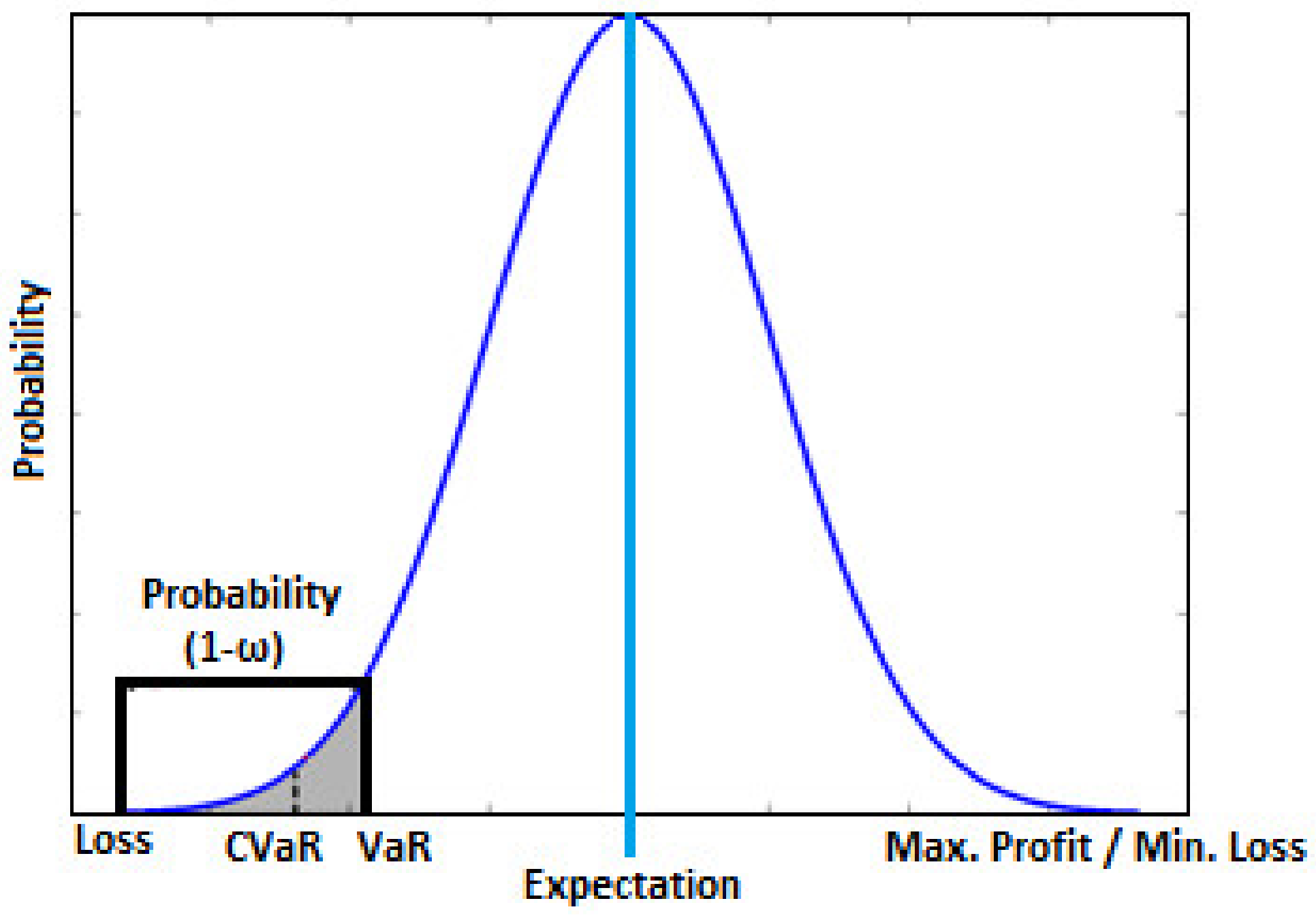
The bus loading sensitivity factor (BLSF) was considered here to determine the utmost profound bus in the system. BLSF is the fraction of the number of lines connected to a bus and the total line present in the network.

$$\mathrm{BLSF}=\frac{{\mathrm{L}}_{\mathrm{BUS}}}{{\mathrm{L}}_{\mathrm{SYS}}}$$

(12)

Here, ‘L_BUS’ is the number of transmission lines connected to a bus. ‘L_SYS’ is the total lines existing in the network. The maximum value of BLSF represents the most sensitive bus in the system.

2.5. VaR and CVaR

VaR and CVaR were used as risk assessment tools. Both assessment tools were worked based on probabilistic studies and the confidence level of assurance (ω). The confidence level is generally 95%, 98%, and 99% for exploring the VaR and CVaR values, whereas 98% was used in this work. CVaR is the more accurate risk measuring tool. With the loss quantity of (1 − ω) percentile, VaR depicts the smallest loss but CVaR shows the average loss components. m(x,y) is the loss components allied to the decision vector P, taken from a definite subset x of $\dot{\mathrm{Q}}$ and the random vector y in $\dot{\mathrm{Q}}$. The probability of loss components m(x,y) is indicated by n(y), which cannot be beyond the threshold limit (ξ) [35]:

$$\mathsf{\beta }\left( \mathrm{x}, \mathsf{\xi }\right)={{\displaystyle \int }}_{\mathrm{m} \left(\mathrm{x},\mathrm{y}\right)\le \mathsf{\xi }}\mathrm{n} \left(y\right)\mathrm{d}\mathsf{\xi }$$

(13)

The mathematical formulation of the assurance level based VaR and CVaR is as follows:

$${\mathsf{\xi }}_{\mathrm{p}}\left(\mathrm{x}\right)=\min \left\{ \mathsf{\xi }ϵ\dot{\mathrm{Q}}: \mathsf{\beta }\left(\mathrm{x}, \mathsf{\xi }\right)\right\}$$

(14)

$${\mathsf{\theta }}_{\mathrm{p}}\left(\mathrm{x}\right)=\frac{1}{1-\omega }\left[\left({\displaystyle \sum }_{\mathrm{c}=1}^{{\mathrm{C}}_{\mathrm{a}}}\left({\mathrm{n}}_{\mathrm{c}}-\omega \right)p_{{\mathrm{c}}_{\mathrm{a}}}\right)+{\displaystyle \sum }_{\mathrm{c}={\mathrm{c}}_{\mathrm{a}}}^{\mathrm{T}}{\mathrm{n}}_{\mathrm{c}}{\mathrm{p}}_{\mathrm{c}}\right]$$

(15)

Here, T is the number of trials composed under numerous conditions.

Figure 3 shows the graphical representation of risk assessment parameters. The maximum negative values of VaR and CvaR depict the maximum system risk. Thus, it is desirable to move towards the right-hand side to minimize the system loss and minimize the system risk.

3. Optimization Techniques

This section exhibits the details of three optimization techniques i.e., Artificial Gorilla Troops Optimizer Algorithm (AGTO), Honey Badger Algorithm (HBA), and Sequential Quadratic Programming (SQP).

3.1. Artificial Gorilla Troops Optimizer Algorithm (AGTO)

An artificial gorilla troop optimizer (AGTO) algorithm is proposed, inspired by the group behavior of gorillas, i.e., gorillas’ group life when finding the food and their group life together. The AGTO algorithm is composed of the following five strategies in which the first three are for the exploration phase, and the last two are for the exploitation phase [36]:

• Migration to unknown areas increases the exploration of AGTO.
• Moving to other gorillas increases the balance between exploration and exploitation.
• Migration towards a known place increases the searching capability in different optimization spaces.
• Follow the silverback (leader for a group that makes decisions and guides others), which maintains the systematic and continued exploration in individual groups to ease exploitation.
• Competition for adult females explains or mimics the group’s expansion fight process by puberty/adult gorillas after choosing adult females.

3.2. Honey Badger Algorithm (HBA)

The HBA is a new-fangled metaheuristic optimization method. The keen foraging performance detected in the honey badger was the main motivation for constructing this algorithm [37]. This method is used to mathematically build an effective search methodology for solving optimization complications. The potent search manner of the honey badger, which uses digging and finding methods, is framed within the HBA as two different stages, i.e., exploration and exploitation.

3.3. Sequential Quadratic Programming (SQP)

In this proposed work the optimal power flow (OPF) problem was described using MATPOWER software. MATPOWER software is a programming software that uses the SQP method to find the OPF of a system. SQP is also the same process as a generalization of the Newton–Raphson method, in which non-linear constrained optimization problems are solved in steps to discover the OPF of the system.

4. Objective Function

The increased power demand and limitations in a new transmission line installation has forced the entire power sector to think about the use of FACTS devices. The installation of FACTS devices can reduce the congestion in the transmission lines, which directly reduces the congestion cost and finally reduces the system generation cost. The use of FACTS devices can also reduce the chances of line failure by providing more thermal limits to the lines. These conditions minimize the system risk. To verify this concept, this work considers both regulated and deregulated power systems.

From the basic impression of deregulation, the system economy always improves under this condition when compared to the regulated system. In this work, two objective functions have been considered:

(i)

Minimization of system risk by improving the values of VaR and CVaR.

(ii)

Minimization of system generation cost.

The mathematical expression of the first objective function is:

$$\mathrm{Max}.{\mathsf{\xi }}_{\mathrm{p}}\left(\mathrm{x}\right)=\min \{ \mathsf{\xi }ϵ\dot{\mathrm{Q}}: \mathsf{\beta }\left(\mathrm{x}, \mathsf{\xi }\right)$$

(16)

$$\mathrm{Max}.{ \mathsf{\theta }}_{\mathrm{p}}\left(\mathrm{x}\right)=\frac{1}{1-\omega }\left[\left({{\displaystyle \sum }}_{\mathrm{c}=1}^{{\mathrm{C}}_{\mathrm{a}}}\left({\mathrm{n}}_{\mathrm{c}}-\omega \right)p_{{\mathrm{c}}_{\mathrm{a}}}\right)+{{\displaystyle \sum }}_{\mathrm{c}={\mathrm{c}}_{\mathrm{a}}}^{\mathrm{T}}{\mathrm{n}}_{\mathrm{c}}{\mathrm{p}}_{\mathrm{c}}\right]$$

(17)

From Figure 3, it is clear that the system risk will be minimized if the values of VaR and CVaR increase. Thus, the first objective function is considered as a maximization problem. The mathematical expression of the second objective function is as follows:

$$\mathrm{Min}. \mathrm{TGCS}\left(\mathrm{i},\mathrm{t}\right)= \mathrm{TGCT}\left(\mathrm{i},\mathrm{t}\right)+ \mathrm{TGCW}\left(\mathrm{i},\mathrm{t}\right)+{ \mathrm{H} \mathrm{Asset} \mathrm{Price}}_{\mathrm{FACTS}}(\mathrm{i},\mathrm{t})$$

(18)

TR(i,t) = TR_T(i,t) + TR_W(i,t)

(19)

$$\mathrm{TRT}\left(\mathrm{i},\mathrm{t}\right)={{\displaystyle \sum }}_{\mathrm{i}=1}^{\mathrm{NG}}{\mathrm{P}}_{\mathrm{G}}\left(\mathrm{i},\mathrm{t}\right)\times \mathrm{LMP}\left(\mathrm{i},\mathrm{t}\right)$$

(20)

Here, ‘TGC_S(i,t)’ is the total generation cost for the i^th unit at time ’t’, which is separated into three portions, i.e., thermal power generation cost (TGC_T(i,t)), wind power generation cost (TGC_W(i,t)), and investment cost of FACTS devices (${\mathrm{HAsset} \mathrm{Price}}_{\mathrm{FACTS}}$(i,t)). Similarly, system revenue (TR(i,t)) is alienated into two portions, i.e., revenue from thermal power (TR_T(i,t)) and revenue from wind farms (TR_W(i,t)). Equation (20) displays the revenue from the thermal power plant, which depends on the thermal power generator (P_G) and LMP at the generator bus (LMP(i,t)). NG is the total number of generators placed in the system. The expression of the thermal generation cost is as follows:

$$\mathrm{TGCT}\left(\mathrm{i},\mathrm{t}\right)={{\displaystyle \sum }}_{\mathrm{i}=1}^{\mathrm{NG}}(\mathrm{a}\times {\mathrm{P}}^2\left(\mathrm{i},\mathrm{t}\right)+\mathrm{b}\times \mathrm{P}\left(\mathrm{i},\mathrm{t}\right)+\mathrm{c})$$

(21)

where, ‘a’, ‘b’, and ‘c’ are the cost coefficients of the thermal generators.

The entire work was performed using MATPOWER software. Only the last section of the work was carried out using MATLAB to solve the OPF problem using AGTO and HBA. To solve the optimal power flow problems, several constraints have been considered, which are shown as follows:

$${\mathrm{V}}_{\mathrm{i}}^{\min }\le {\mathrm{V}}_{\mathrm{i}}\le {\mathrm{V}}_{\mathrm{i}}^{\max },\mathrm{i}=1,2,3, \dots \mathrm{NB}$$

(22)

$${\mathsf{\phi }}_{\mathrm{i}}^{\min }\le {\mathsf{\phi }}_{\mathrm{i}}\le {\mathsf{\phi }}_{\mathrm{i}}^{\max },\mathrm{i}=1,2,3, \dots \mathrm{NB}$$

(23)

$${\mathrm{TL}}_{\mathrm{l}}\le {\mathrm{TL}}_{\mathrm{l}}^{\max }, \mathrm{l}=1,2,3,\dots {\mathrm{N}}_{\mathrm{d}}$$

(24)

$${\mathrm{P}}_{{\mathrm{G}}_{\mathrm{i}}}^{\min }\le {\mathrm{P}}_{{\mathrm{G}}_{\mathrm{i}}}\le {\mathrm{P}}_{{\mathrm{G}}_{\mathrm{i}}}^{\max },\mathrm{i}=1,2,3, \dots \mathrm{NB}$$

(25)

$${\mathrm{Q}}_{{\mathrm{G}}_{\mathrm{i}}}^{\min }\le {\mathrm{Q}}_{{\mathrm{G}}_{\mathrm{i}}}\le {\mathrm{Q}}_{{\mathrm{G}}_{\mathrm{i}}}^{\max },\mathrm{i}=1,2,3, \dots \mathrm{NB}$$

(26)

$${\mathrm{L}}_{\mathrm{TCSC}}^{\min }\le {\mathrm{L}}_{\mathrm{TCSC}}\le {\mathrm{L}}_{\mathrm{TCSC}}^{\max }$$

(27)

$${\mathrm{L}}_{\mathrm{UPFC}}^{\min }\le {\mathrm{L}}_{\mathrm{UPFC}}\le {\mathrm{L}}_{\mathrm{UPFC}}^{\max }$$

(28)

$${\mathrm{N}}_{\mathrm{UPFC}}^{\min }\le {\mathrm{N}}_{\mathrm{UPFC}}\le {\mathrm{N}}_{\mathrm{UPFC}}^{\max }$$

(29)

Here, P_Gi is the power generation at ith generation unit. The voltage magnitude is represented by $\left|{\mathrm{V}}_{\mathrm{i}}\right|$ of bus i. The voltage angle is represented by ${\mathsf{\delta }}_{\mathrm{i}}$ of the bus i. The real and reactive power are ${\mathrm{P}}_{\mathrm{Gi}}$ and ${\mathrm{Q}}_{\mathrm{Gi}}$, which flow through the system through bus i. Here, ${\mathrm{P}}_{\mathrm{gi}}^{\max }$, ${\mathrm{P}}_{\mathrm{gi}}^{\min }$ and ${\mathrm{Q}}_{\mathrm{gi}}^{\max }$,${ \mathrm{Q}}_{\mathrm{gi}}^{\min }$ are the maximum and minimum limits of real and reactive powers for bus-i. For bus i, upper voltage and lower voltage limits are represented by ${\mathrm{V}}_{\mathrm{i}}^{\max }$ and ${\mathrm{V}}_{\mathrm{i}}^{\min }.{\mathsf{\varphi }}_{\mathrm{i}}^{\max }$ and ${\mathsf{\varphi }}_{\mathrm{i}}^{\min }$ are the upper and lower phase angle limits of voltage for bus i. The maximum power flow in line l is represented by ${ \mathrm{TL}}_1^{\max }$. The indication flow chart of the presented approach is shown in Figure 4.

5. Results and Discussions

The modified IEEE 14-bus and modified IEEE 30-bus test systems were chosen to verify the effectiveness of the presented approach. The modified IEEE 14-bus system consists of 5 generators, 14 buses, 10 loads, and 20 transmission lines, whereas 6 generators, 30 buses, 21 loads, and 41 transmission lines are present in the modified IEEE 30-bus system. An amount of 100 MVA was chosen as the base MVA, and bus number 1 was considered as the slack bus for both of the considered systems [21,35]. There are five steps involved for completing the entire work, which are as follows:

Step 1 Impact of FACTS device placement in the regulated systems.

Step 2 Impact of FACTS device placement in the deregulated systems.

Step 3 Calculate the system risk in terms of VaR and CVaR and chose the worst case.

Step 4 Placement of wind farm and check the system risk and economic factors using SQP.

Step 5 Operation of FACTS devices alongside the wind farm and check the system risk and economic factors using SQP.

Step 6: Comparison of system risk and economic parameters with different optimization methods.

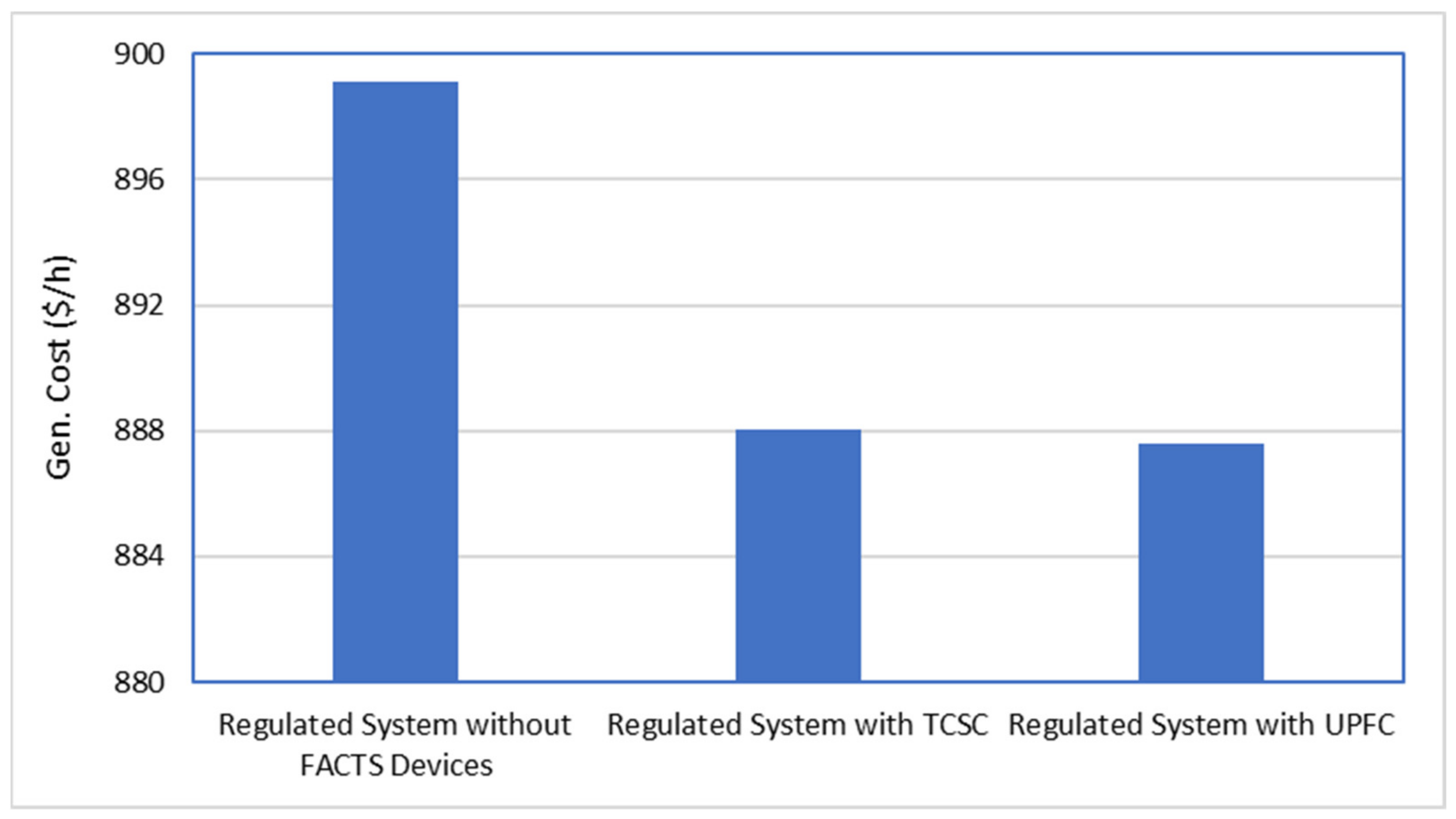
5.1. Impact of FACTS Devices in a Regulated System for the Modified IEEE 14-Bus System

In this step, the impact of TCSC and UPFC devices under a regulated power system was studied concerning the modified IEEE 14 bus system. To do this, the TCSC was placed on every line of the system while varying the compensation level. The minimum generation cost achieved was based on ‘find the optimal position and ratings of TCSC’. Observations from

Table 1. System economy with and without TCSC for the IEEE 14-bus regulated system.

Base Case [20]		with TCSC
Gen. Cost ($/h)	Revenue ($/h)	Opt. Loc. of TCSC at Line No.	LTCSC	Thermal Gen. Cost ($/h)	TCSC Investment Cost ($/h)	Total Gen. Cost ($/h)	Revenue ($/h)
899.09	1226.182	4	−0.55	887.121898	0.933067	888.05496	1292.774

show that the optimal position of TCSC placement was on line number 4, giving minimum generation cost. While integrating the TCSC, the investment cost of TCSC was also considered, as per Equations (6) and (11). Table 1 shows the system generation cost with and without TCSC placement.

From Table 1, it can be observed that the total generation cost is reduced by 11.03504 $/h after the placement of TCSC on line number 4, with a TCSC compensation level of −0.55. Table 1 also shows the revenue of the overall system before and after the placement of TCSC on line number 4. From Table 1, the revenue of the overall system is reduced after the placement of TCSC. To calculate the revenue of the system, LMP is used here.

Like TCSC, the optimal placement of UPFC was also calculated for the modified IEEE 14 bus system.

Table 2. System economy with and without UPFC for the IEEE 14-bus regulated system.

Base Case [20]		with UPFC
Gen. Cost ($/h)	Revenue ($/h)	Opt. Loc. of UPFC at Line No.	Opt. Loc. of Ninj at Bus No.	LUPFC	NUPFC	Thermal Gen. Cost ($/h)	UPFC Investment Cost ($/h)	Total Gen. Cost ($/h)	Revenue ($/h)
899.09	1226.182	4	2	−0.7	2	884.50665	3.087367	887.5940	1294.476

shows the optimal placement and parameter setting of UPFC along with the comparative results of system economy, with and without UPFC placement. To find the optimal location of UPFC in a modified IEEE 14 bus system, system generation cost is calculated after placement of UPFC at each bus.

From Table 2, it is also observed that optimal placement values of UPFC were −0.7 ohm and 2 VAR. Concerning the system generation cost, it is observed that line 4 with bus number 2 gave the minimum system generation cost. Thus, UPFC was placed on line number 4 using bus number 2. From Table 2, the total system generation cost with UPFC was 887.5940 $/h, and without UPFC, was 899.09 $/h. Therefore, the optimal placement of UPFC reduces the system generation cost by 11.496 $/h. To calculate the total system generation cost, UPFC cost was also considered as per Equations (7) and (11). Figure 5 depicts the overall system generation cost with and without FACTS devices. From Figure 6, it is observed that optimal integration of UPFC gives the lowest generation cost when compared to the optimal integration of TCSC in a modified IEEE 14 bus system under a regulated power system.

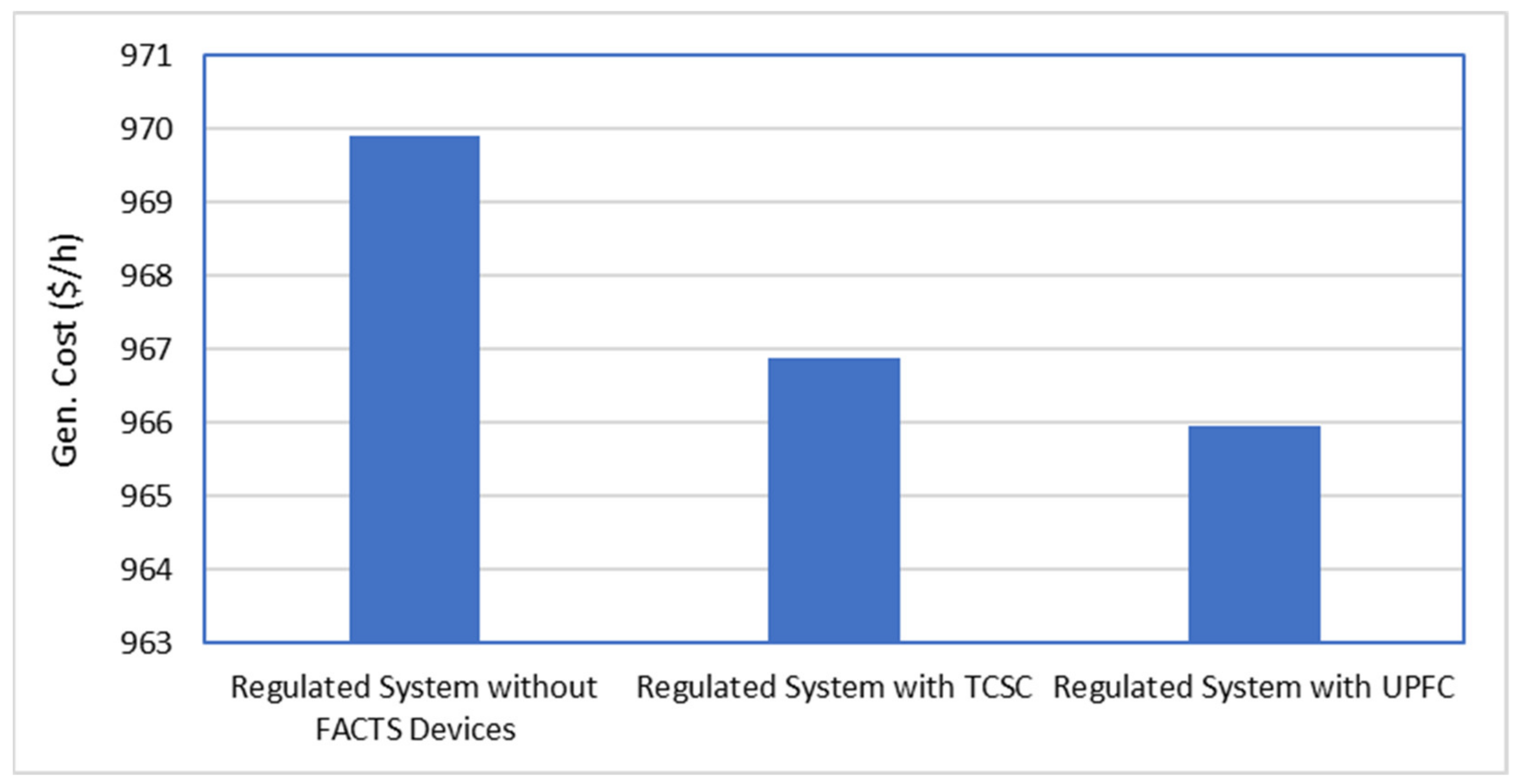
5.2. Impact of FACTS Devices in a Regulated System for Modified IEEE 30-Bus System

The impact of TCSC and UPFC devices under a regulated power system was studied with regards to the modified IEEE 30 bus system for this step. To do this, the optimal placement of TCSC was initially placed on line number 41, based on the minimum generation cost of the system.

Table 3. System economy with and without TCSC for the IEEE 30-bus regulated system.

Base Case [20]		with TCSC
Gen. Cost ($/h)	Revenue ($/h)	Opt. Loc. of TCSC at Line No.	LTCSC	Thermal Gen. Cost ($/h)	TCSC Investment Cost ($/h)	Total Gen. Cost ($/h)	Revenue ($/h)
969.91	1312.604	41	−0.7	966.875852	0.007570	966.883422	1320.524

shows the system generation cost with and without TCSC placement.

From Table 3, it is observed that the total generation cost for the modified IEEE 30 bus system was reduced by 3.03657 $/h after the placement of TCSC on line number 41 with a −0.7 ohm reactance value. Since the modified IEEE 30 bus is a big system, the integration of a single TCSC did not affect total generation cost very much. If we integrate multiple TCSCs in the system, then more system generation cost reductions will occur. Table 3 also shows the revenue for the overall system before and after the placement of TCSC on line number 41. From Table 3, the revenue of the overall system was maximized after the optimal placement of TCSC in the system.

Table 4. System economy with and without UPFC for the IEEE 30-bus regulated system.

Base Case [20]		with UPFC
Gen. Cost ($/h)	Revenue ($/h)	Opt. Loc. of UPFC at Line No.	Opt. Loc. of Ninj at Bus No.	LUPFC	NUPFC	Thermal Gen. Cost ($/h)	UPFC Investment Cost ($/h)	Total Gen. Cost ($/h)	Revenue ($/h)
969.91	1312.604	28	10	0.2	−10	965.90837	0.046346	965.9547	1322.605

shows the system generation cost with and without UPFC device placement on line number 4 and bus number 2. To find the optimal location of UPFC in a modified IEEE 30 bus system, system generation cost was calculated after the placement of UPFC on each bus. From Table 4, it can be seen that the optimal values of UPFC were 0.2 ohms and −10 VAR. Concerning the system generation cost, line 28 with bus no 10 gave minimal system generation cost compared to the other positions of UPFC in the system. Thus, UPFC was placed on line number 28 and bus number 10. From Table 4, the total system generation cost without UPFC was 969.92 $/h, and with UPFC was 965.9547 $/h. Therefore, the optimal placement of UPFC reduced the total system generation cost by 3.9653 $/h. Figure 6 depicts the overall system generation cost with and without FACTS devices for the IEEE 30-bus regulated system. From Figure 7, it can be seen that the optimal integration of UPFC gives the lowest generation cost when compared to the optimal integration of TCSC in a modified IEEE 30 bus system.

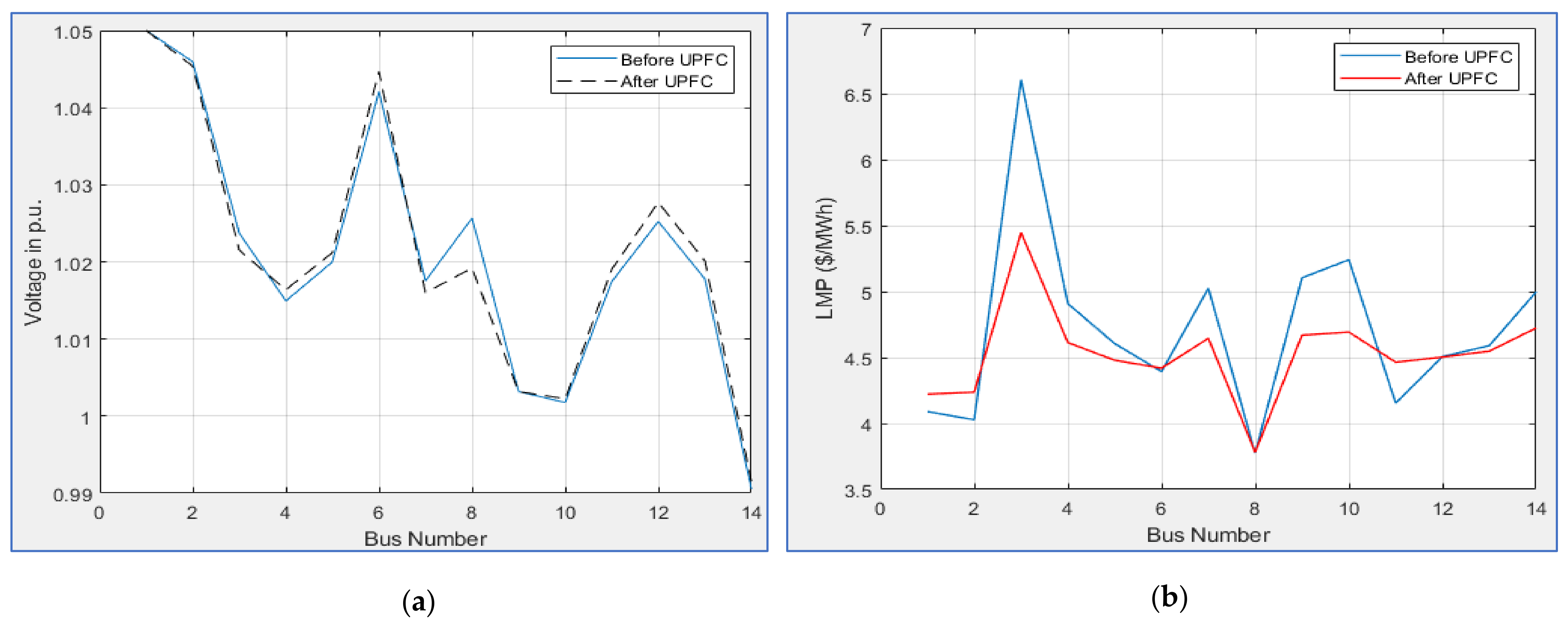
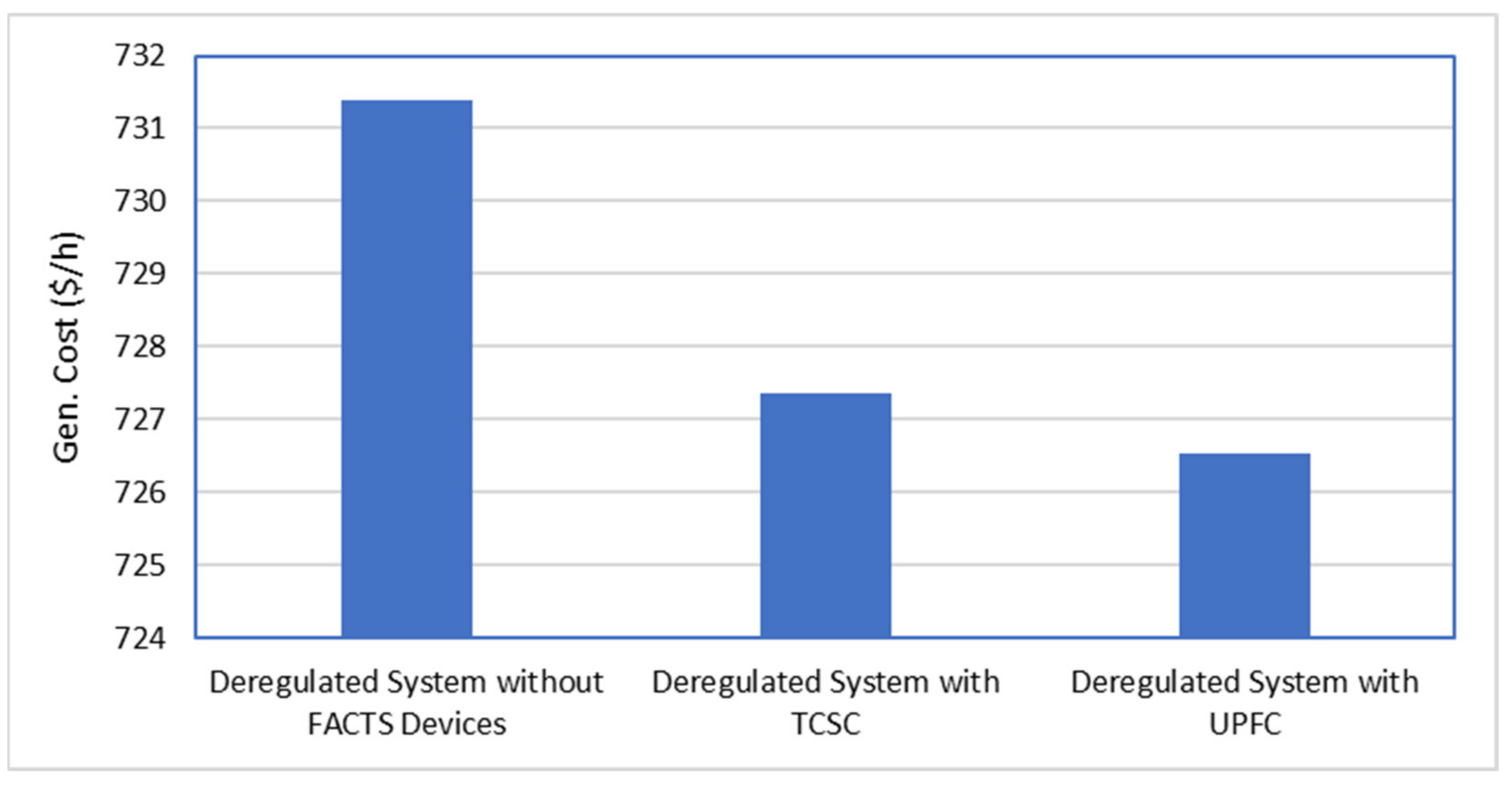
5.3. Impact of FACTS Devices in a Deregulated System for Modified IEEE 14-Bus System

For this step, the impact of TCSC and UPFC devices was studied considering the modified IEEE 14 bus system under a deregulated power system. In this case, bus number five was considered for the deregulated system. For the optimal locations of TCSC and UPFC, a deregulated power system approach was used.

Table 5. System economy with and without TCSC for the IEEE 14-bus deregulated system.

without TCSC		with TCSC
Gen. Cost ($/h)	Revenue ($/h)	Opt. Loc. of TCSC at Line No.	LTCSC	Thermal Gen. Cost ($/h)	TCSC Investment Cost ($/h)	Total Gen. Cost ($/h)	Revenue ($/h)
784.73	1158.069	4	−0.55	772.843737	0.482298	773.326035	1228.083

shows the system generation cost with and without TCSC placement under a deregulated power system.

From Table 5, it can be observed that, after placement of TCSC on line number 4, the total generation cost was reduced from 784.73 $/h to 773.326035 $/h. To achieve this optimal generation cost, a TCSC compensation level of −0.55 was used. From Table 5, the revenue of the overall system improved from 1158.069 $/h to 1228.083 $/h after the placement of TCSC on line number 4. Figure 7 shows the voltage and LMP value of the deregulated power system before and after placement of TCSC. From Figure 7, it can be observed that the maximum bus, system voltage, and LMP values were reduced after the integration of TCSC on line number 4 under a deregulated power system.

Figure 8 shows the voltage and LMP value of the deregulated power system before and after placement of UPFC. From Figure 8, it can be observed that the maximum bus, system voltage, and LMP values were reduced after the integration of UPFC on line number 4 and bus number 2 under a deregulated power system (shown in

Table 6. System economy with and without UPFC for the IEEE 14-bus deregulated system.

without UPFC		with UPFC
Gen. Cost ($/h)	Revenue ($/h)	Opt. Loc. of UPFC at Line No.	Opt. Loc. of Ninj at Bus No.	LUPFC	NUPFC	Thermal Gen. Cost ($/h)	UPFC Investment Cost ($/h)	Total Gen. Cost ($/h)	Revenue ($/h)
784.73	1158.069	4	2	−0.7	2	769.31535	3.343308	772.6586	1230.131

).

Figure 9 depicts the overall system generation cost with and without the integration of TCSC and UPFC in a modified IEEE 14-bus system under a deregulated power system. From Figure 9, it can be observed that the optimal integration of UPFC gives the least generation cost compared to the optimal integration of TCSC in a modified IEEE 14 bus system under a deregulated power system.

5.4. Impact of FACTS Devices in a Deregulated System for Modified IEEE 30-Bus System

For this step, the impact of TCSC and UPFC devices was studied with reagrds to the modified IEEE 30 bus system under a deregulated power system. In this case, bus numbers 4 and 7 were considered for deregulation. Similar to the regulated power systems, the same approach was used in the deregulated power system for the optimal location of TCSC and UPFC.

Table 7. System economy with and without TCSC for IEEE 30-bus deregulated system.

without TCSC		with TCSC
Gen. Cost ($/h)	Revenue ($/h)	Opt. Loc. of TCSC at Line No.	LTCSC	Thermal Gen. Cost ($/h)	TCSC Investment Cost ($/h)	Total Gen. Cost ($/h)	Revenue ($/h)
731.39	1172.377	24	−0.7	727.357248	0.002102	727.359350	1182.321

and

Table 8. System economy with and without UPFC for the IEEE 30-bus deregulated system.

without UPFC		with UPFC
Gen. Cost ($/h)	Revenue ($/h)	Opt. Loc. of UPFC at Line No.	Opt. Loc. of Ninj at Bus No.	LUPFC	NUPFC	Thermal Gen. Cost ($/h)	UPFC Investment Cost ($/h)	Total Gen. Cost ($/h)	Revenue ($/h)
731.39	1172.377	41	6	−0.7	−6	726.33555	0.197623	726.5331	1186.325

, respectively, show the system generation cost with and without integration of TCSC and UPFC under a deregulated power system.

From Table 7, it can be seen that, after the placement of TCSC on line number 24, the total generation cost was reduced from 731.39 $/h to 727.359350 $/h. From Table 7, the revenue of the overall system improved by 9.944 $/h after the placement of TCSC on line number 24 under a deregulated power system. From Table 8, it can be observed that after the placement of UPFC on line number 41 and bus number 6, under a deregulated power system, the total generation cost was reduced from 731.39 $/h to 726.5331 $/h. From Table 8, the revenue of the overall system improved from 1171.377 $/h to 1186.325 $/h after the optimal placement of UPFC under a deregulated power system.

Figure 10 shows the overall system generation cost with and without the integration of TCSC and UPFC for a modified IEEE 30-bus system under a deregulated power system. From Figure 10, it can be seen that the optimal integration of UPFC gave the lowest generation cost when compared to the optimal integration of TCSC in a modified IEEE 30 bus system under a deregulated power system.

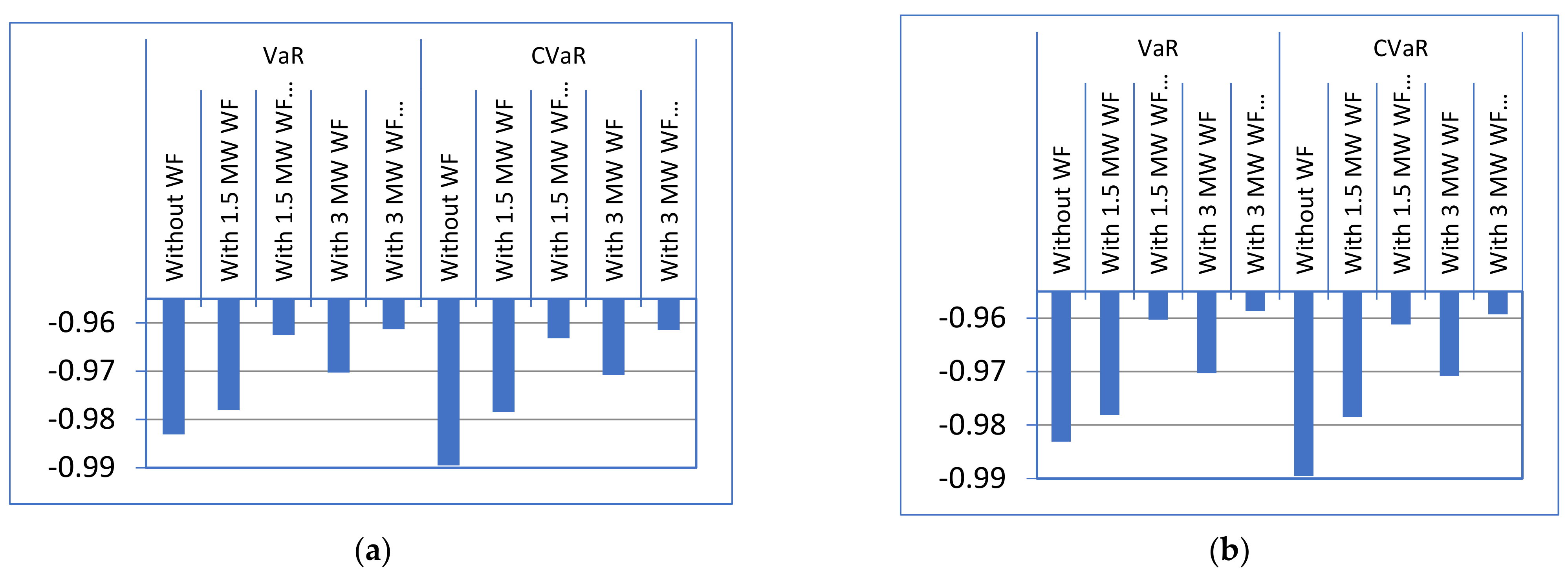
5.5. Calculate the System Risk in Terms of VaR and CVaR

An electrical system faces lots of problems when maintaining its stability and security. There is always a chance of failure in the generators, transmission lines, and buses or a sudden increment in the power demand. To make the proposed approach more accurate in real-time, a total number of 50 scenarios have been generated for this work by considering different line outages, bus outages, load increments, and combinations of all of these factors. After creating several scenarios, the risk assessment parameters (i.e., VaR and CVaR) measured all cases to find the riskiest conditions based on the values of VaR and CVaR.

Table 9. System risk in the modified IEEE 14-bus system.

Sl. No.	Transmission Line Outage	Risk Assessment Parameters		Rank
		VaR	CVaR
1	05–06	−0.9825	−1.0917	1
2	04–09	−0.9741	−1.0823	2
3	06–11	−0.9676	−1.075	3
4	06–13	−0.9669	−1.0743	4
5	13–14	−0.9665	−1.074	5

and

Table 10. System risk in the modified IEEE 30-bus system.

Sl. No.	Transmission Line Outage	Risk Assessment Parameters		Rank
		VaR	CVaR
1	01–02	−0.9831	−0.9895	1
2	09–10	−0.9817	−0.9820	2
3	01–03	−0.9752	−0.9768	3
4	10–20	−0.9738	−0.9741	4
5	06–10	−0.9726	−0.9732	5

show the top 5 cases based on the highest system risk for the modified IEEE-14 and IEEE-30 bus systems, respectively. It was found that the line outage of 05–06 and 01–02 creates the maximum system risk for the IEEE-14 and IEEE-30 bus systems. Thus, these two cases were chosen as the worst conditions for the considered systems. The system risk was calculated with a confidence level of 98%.

The next steps of the work were performed using the considered worst cases only. If the system risk and economic parameters improve with the incorporation of the proposed methodology, then better results will be obtained for the less risky scenarios.

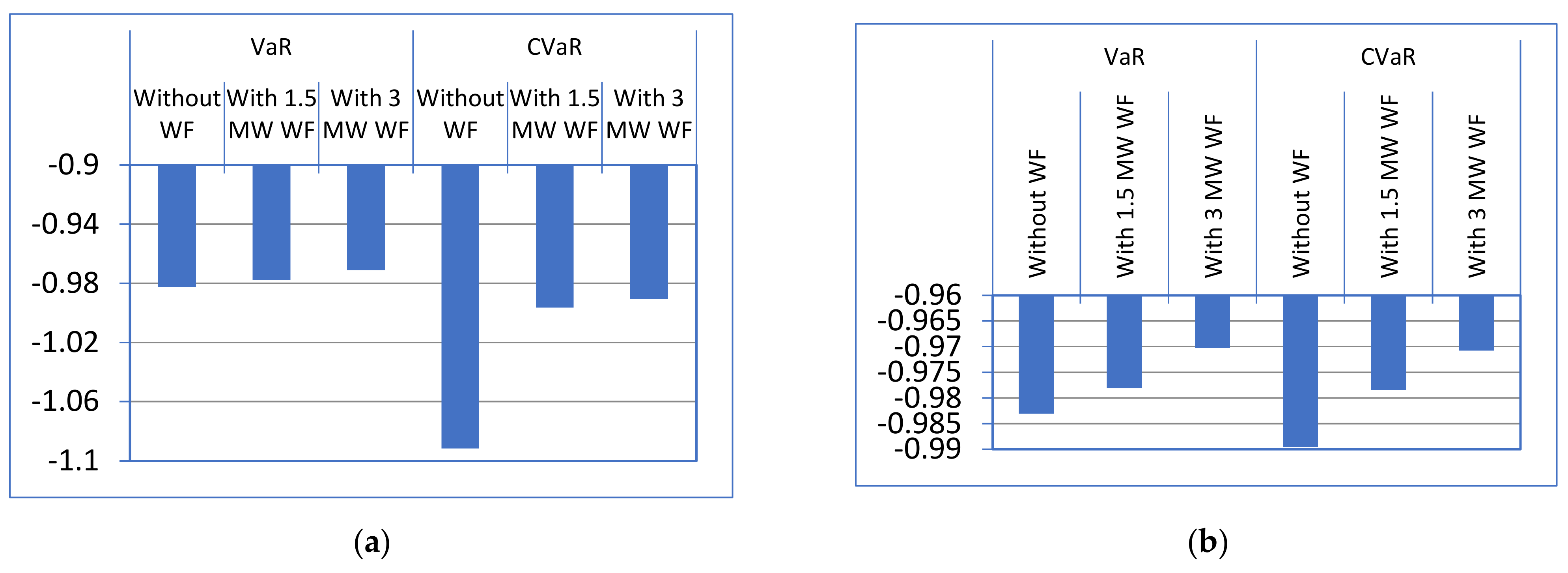
5.6. Placement of Wind Farm and Check the System Risk and Economic Factors Using SQP

The bus loading sensitivity factor (BLSF) was used to identify the most sensitive bus in the system. The wind farm was placed under the most sensitive bus of the system to get the maximum benefits.

Table 11. Bus loading sensitivity factor (BLSF) for the modified IEEE 14-bus system.

Bus No.	Bus Loading Sensitivity Factor (BLSF)	Bus No.	Bus Loading Sensitivity Factor (BLSF)	Bus No.	Bus Loading Sensitivity Factor (BLSF)
1	0.1	6	0.2	11	0.1
2	0.2	7	0.15	12	0.1
3	0.05	8	0.05	13	0.15
4	0.25	9	0.2	14	0.1
5	0.2	10	0.1

and

Table 12. Bus loading sensitivity factor (BLSF) for the modified IEEE 30-bus system.

Bus No.	Bus Loading Sensitivity Factor (BLSF)	Bus No.	Bus Loading Sensitivity Factor (BLSF)	Bus No.	Bus Loading Sensitivity Factor (BLSF)
1	0.049	11	0.024	21	0.049
2	0.098	12	0.122	22	0.073
3	0.024	13	0.024	23	0.049
4	0.098	14	0.049	24	0.073
5	0.049	15	0.098	25	0.073
6	0.171	16	0.049	26	0.024
7	0.049	17	0.049	27	0.098
8	0.049	18	0.049	28	0.073
9	0.073	19	0.049	29	0.049
10	0.146	20	0.049	30	0.049

show the ranking of BLSF for the modified IEEE-14 and IEEE-30 bus systems, respectively. From these tables, it was found that bus numbers 4 and 6 were the most sensitive buses for the two considered system, respectively. Therefore, the wind farm was placed under these buses, i.e., bus number 4 for the IEEE 14-bus system and bus number 6 for the IEEE 30-bus system.

The optimal placement of a wind farm provides additional safety to the electrical system by providing extra generated power. From Figure 4, it is clear that negative maximum values of VaR and CVaR represent minimum profit and maximum risk for the power system. It is desirable to move the values of VaR and CVaR towards the right-hand side to provide maximum profit.

Table 13. VaR and CVaR after Installation of a wind farm in the IEEE 14-bus and 30-bus system.

Case	Outage Line	Wind Farm Placed at Bus No.	Wind Power Quantity (MW)	System Generation Cost before Placement of Wind Farm ($/h)	System Generation Cost after Placement of Wind Farm ($/h)	Risk Parameter before Wind Farm Placement		Risk Parameter after Wind Farm Placement
						VaR	CVaR	VaR	CVaR
IEEE 14-bus system	05–06	4	1.5	785.23	781.485	−0.9825	−1.0917	−0.9778	−0.9965
			3		779.79			−0.9712	−0.9907
IEEE 30-bus system	01–02	6	1.5	733.94	732.45	−0.9831	−0.9895	−0.9781	−0.9785
			3		731.01			−0.9703	−0.9708

shows the VaR and CVaR values after the installation of the wind farm under the IEEE 14-bus and 30-bus systems. To show the variable nature of wind power, two different quantities of wind power (i.e., 1.5 and 3 MW) were incorporated into the system. From the results, it can be seen that the system risk is minimized after the placement of maximum quantities of wind farms in the system. The system generation cost also follows under the same conditions. The maximum quantities of wind power provide a minimum generation cost-based system.

The comparative studies on system risk with and without the placement of wind farms under the IEEE 14-bus and IEEE 30-bus systems are shown in Figure 11. It can be seen that VaR and CVaR were −0.9825 and −1.0917, respectively, for the IEEE 14-bus system, whereas this reduced to −0.9712 and −0.9907, respectively, after the placement of the 3 MW wind farm on bus number 4. The same results arose for the IEEE 30-bus system. Thus, it can conclude that the placement of WFs provides both risk minimization and generation cost minimization for any power system.

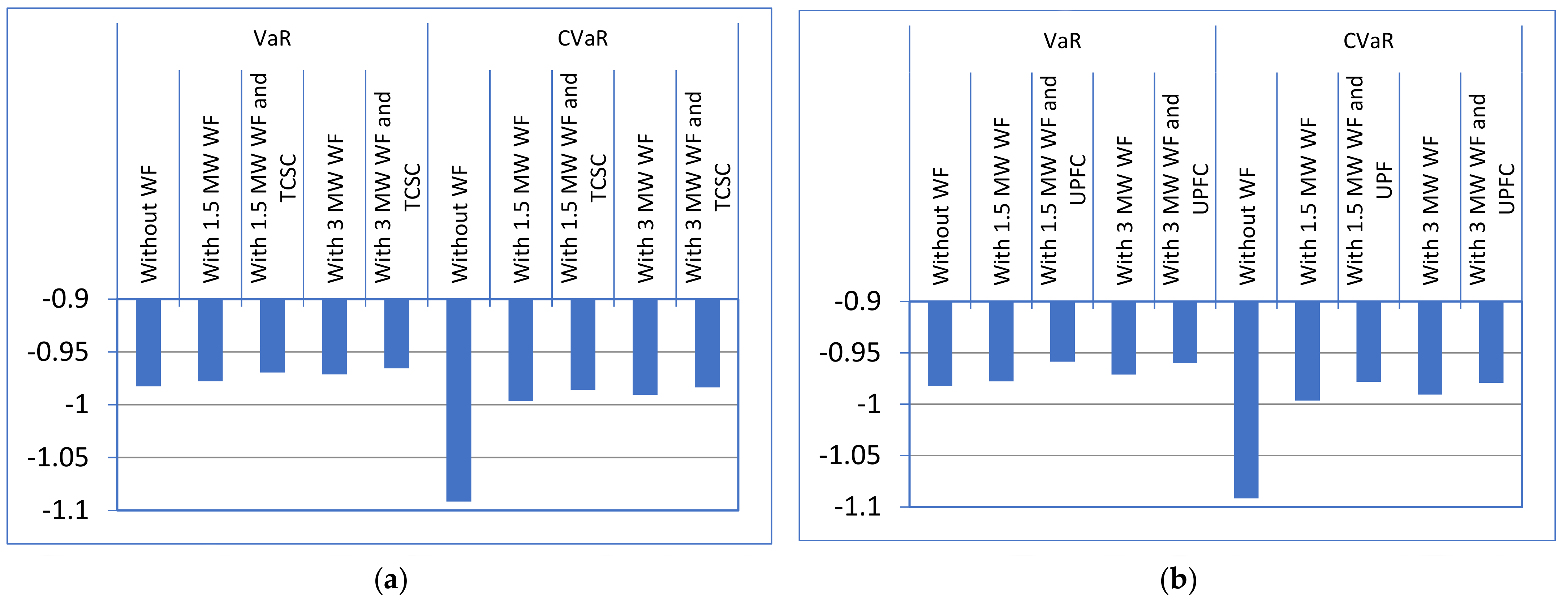
5.7. Operation of FACTS Devices along with Wind Farm and Check the System Risk and Economic Factors Using SQP for Deregulated System

In this part of the work, the FACTS devices were operated alongside the wind farm.

Table 14. VaR and CVaR after installation of a wind farm and FACTS devices in the IEEE 14-bus system.

FACTS Device	Outage Line	Wind Farm Placed at Bus No.	Wind Power Quantity (MW)	FACTS Device Placed at Line No.	System Generation Cost after Wind Farm Placement but without FACTS Devices ($/h)	System Generation Cost after Wind Farm and FACTS Devices Placement ($/h)	Risk Parameter after Wind Farm Placement but without FACTS Devices		Risk Parameter after Wind Farm and FACTS Devices Placement
							VaR	CVaR	VaR	CVaR
TCSC	05–06	4	1.5	4	781.485	780.259	−0.9778	−0.9965	−0.9695	−0.9857
			3		779.79	778.354	−0.9712	−0.9907	−0.9656	−0.9836
UPFC			1.5	4	781.485	780.038	−0.9778	−0.9965	−0.9587	−0.9783
			3		779.79	777.962	−0.9712	−0.9907	−0.9603	−0.9792

depicts the values of risk assessment parameters along with the system generation cost before and after placement of TCSC and UPFC alongside the wind farm. The FACTS devices can maximize the thermal limit of the transmission line, which can cause the minimization of system congestion. The system generation cost is minimized with the minimization of system congestion. On other hand, the system risk has also been minimized with the reduction of the system congestion. From Table 14 and Figure 12, it is clear that the system risk was reduced by a large quantity under the hybrid operation of the wind farm with UPFC in the IEEE 14-bus system.

A higher quantity of wind farms provides the least system generation cost, which will increase social benefits. Like the IEEE 14-bus system, the system generation cost and system risk also improved for the IEEE 30-bus system, which is shown in

Table 15. VaR and CVaR after installation of the wind farm and FACTS devices in the IEEE 30-bus system.

FACTS Device	Outage Line	Wind Farm Placed at Bus No.	Wind Power Quantity (MW)	FACTS Device Placed at Line No.	System Generation Cost after Wind Farm Placement but without FACTS Devices ($/h)	System Generation Cost after Wind Farm and FACTS Devices Placement ($/h)	Risk Parameter after Wind Farm Placement but without FACTS Devices		Risk Parameter after Wind Farm and FACTS Devices Placement
							VaR	CVaR	VaR	CVaR
TCSC	01–02	6	1.5	24	732.45	731.135	−0.9781	−0.9785	−0.9625	−0.9632
			3		731.01	729.934	−0.9703	−0.9708	−0.9613	−0.9615
UPFC			1.5	41	732.45	730.952	−0.9781	−0.9785	−0.9603	−0.9612
			3		731.01	729.264	−0.9703	−0.9708	−0.9587	−0.9593

and Figure 13.

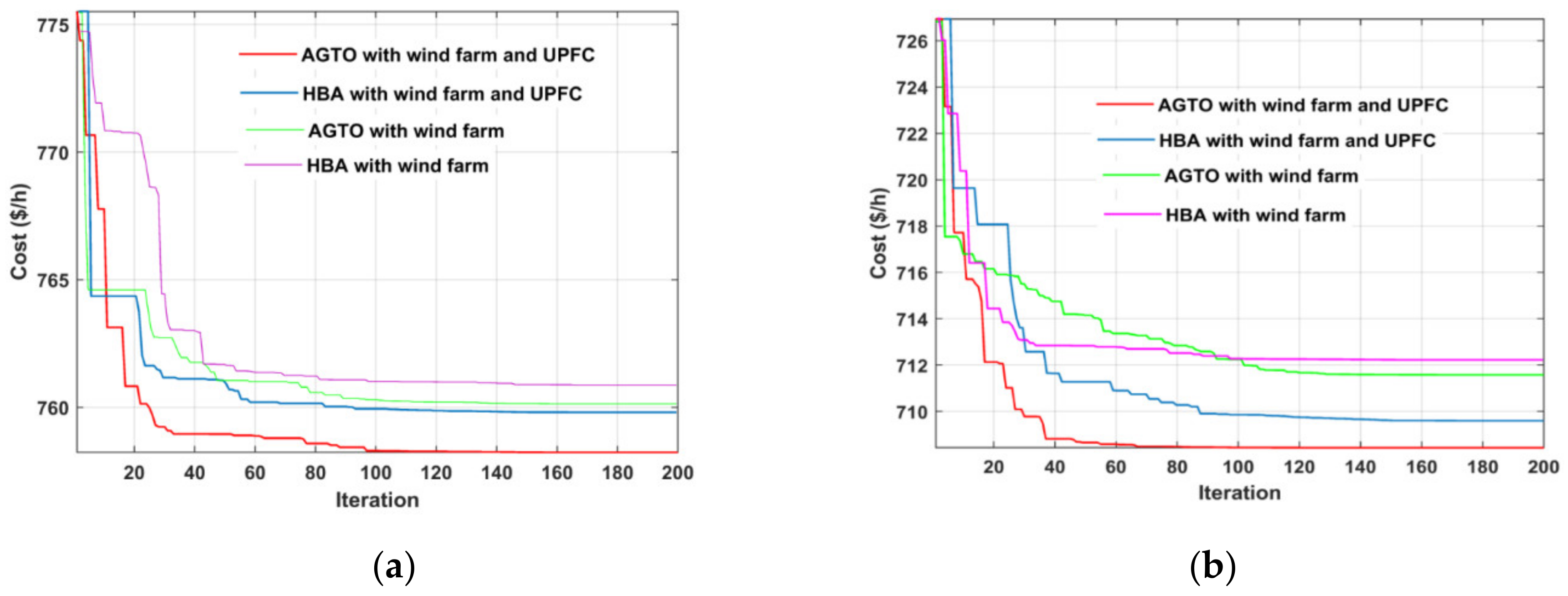
5.8. Comparison of Economic Parameters with Different Optimization Methods

The first five steps were performed using sequential quadratic programming. Now, in this step, two additional optimization techniques named Artificial Gorilla Troops Optimizer Algorithm (AGTO) and Honey Badger Algorithm (HBA) were used to verify the application of the presented approach.

Table 16. System generation cost with different optimization techniques for the IEEE 14-bus and IEEE 30-bus systems.

System Details	Wind Farm Placed at Bus No. and Wind Power Quantity	Generation Cost after WF Placement but without FACTS ($/h) Using SQP	Generation Cost after WF Placement but without FACTS ($/h) Using AGTO	Generation Cost after WF Placement but without FACTS ($/h) Using HBA	System Generation Cost after Wind Farm and TCSC ($/h) Using SQP	System Generation Cost after Wind Farm and TCSC ($/h) Using AGTO	System Generation Cost after Wind Farm and TCSC ($/h) Using HBA	System Generation Cost after Wind Farm and UPFC ($/h) Using SQP	System Generation Cost after Wind Farm and UPFC ($/h) Using AGTO	System Generation Cost after Wind Farm and UPFC ($/h) Using HBA
IEEE 14-bus system	Bus No. 4 with 3 MW	779.79	760.24	761.26	778.354	759.05	760.24	777.962	758.53	759.62
IEEE 30-bus system	Bus No. 6 with 3 MW	731.01	711.56	712.43	729.934	709.95	710.86	729.264	708.65	709.74

shows the comparative results of system economy for selected cases in the deregulated environment. From the results, it can be seen that the AGTO algorithm provides better results among all the applied optimization methods. Figure 14 displays the comparative convergence plot of AGTO and HBA algorithms for the modified IEEE 14-bus and IEEE-30 bus systems, considering a 3 MW wind farm and UPFC.

From the comparative convergence curve, we can observe that the AGTO algorithm gave better results compared to the HBA algorithm. After the application of the presented method, it can be concluded that the optimal placement of wind farms and FACTS devices provides the most secured system, which minimizes the generation cost as well as system risk mitigation. Among SQP, AGTO, and HBA, the system economy performs best using AGTO. Due to the novel features of AGTO regarding local and global minima calculations, this constitutes the most effective optimization technique for this selected area of the research.

6. Conclusions

The cooperative effect of wind farms and FACTS devices on the economic efficiency of a power system are explored in this paper. To validate the work, both regulated and unregulated market environments were chosen. Value at risk (VaR) and cumulative value at risk (CVaR) were used to evaluate the system risk. The minimization of system risk can improve the stability and security of any electrical system. The bus loading sensitivity factor (BLSF) was used to identify the most sensitive bus in the considered system, concerning where the wind farm had been placed for maximum effect on the electrical system. The optimal position and ratings of the FACTS devices were identified by considering the minimum generation cost of the system. To examine the effect of system risk regarding wind farms and FACTS devices under a deregulated power system, comparative studies were conducted using different optimization techniques such as the Artificial Gorilla Troops Optimizer Algorithm (AGTO), Honey Badger Algorithm (HBA), and Sequential Quadratic Program-ming (SQP). The modified IEEE 14-bus system and modified IEEE 30-bus system were used here to analyze the efficiency and robustness of the presented work. As evident from the results, the presence of TCSC and UPSC when using a wind farm decreases the economic parameters of the system by reducing the system risk. Artificial gorilla troops optimizer algorithm (AGTO) was used for the first time in this kind of risk mitigation problem, which constitutes the uniqueness of this paper.

References

1. Hussain, S.M.S.; Nadeem, F.; Aftab, M.A.; Ali, I.; Ustun, T.S. The Emerging Energy Internet: Architecture, Benefits, Challenges, and Future Prospects. Electronics 2019, 8, 1037. [Google Scholar] [CrossRef] [Green Version]
2. Ustun, T.S.; Aoto, Y. Analysis of Smart Inverter’s Impact on the Distribution Network Operation. IEEE Access 2019, 7, 9790–9804. [Google Scholar] [CrossRef]
3. Elmitwally, A.; Eladl, A. Planning of multi-type FACTS devices in restructured power systems with wind generation. Int. J. Electr. Power Energy Syst. 2016, 77, 33–42. [Google Scholar] [CrossRef]
4. Arango-Aramburo, S.; Bernal-García, S.; Larsen, E.R. Renewable energy sources and the cycles in deregulated electricity markets. Energy 2021, 223, 120058. [Google Scholar] [CrossRef]
5. Dawn, S.; Tiwari, P.K. Improvement of economic profit by optimal allocation of TCSC & UPFC with wind power generators in double auction competitive power market. Int. J. Electr. Power Energy Syst. 2016, 80, 190–201. [Google Scholar]
6. Abdolrasol, M.G.M.; Hussain, S.M.S.; Ustun, T.S.; Sarker, M.R.; Hannan, M.A.; Mohamed, R.; Ali, J.A.; Mekhilef, S.; Milad, A. Artificial Neural Networks Based Optimization Techniques: A Review. Electronics 2021, 10, 2689. [Google Scholar] [CrossRef]
7. Latif, A.; Hussain, S.M.S.; Das, D.C.; Ustun, T.S. Double stage controller optimization for load frequency stabilization in hybrid wind-ocean wave energy based maritime microgrid system. Appl. Energy 2021, 282, 116–171. [Google Scholar] [CrossRef]
8. Latif, A.; Hussain, S.M.S.; Das, D.C.; Ustun, T.S. Optimum Synthesis of a BOA Optimized Novel Dual-Stage PI − (1 + ID) Controller for Frequency Response of a Microgrid. Energies 2020, 13, 3446. [Google Scholar] [CrossRef]
9. Singh, S.; Chauhan, P.; Aftab, M.A.; Ali, I.; Hussain, S.M.S.; Ustun, T.S. Cost Optimization of a Stand-Alone Hybrid Energy System with Fuel Cell and PV. Energies 2020, 13, 1295. [Google Scholar] [CrossRef] [Green Version]
10. Dey, P.P.; Das, D.C.; Latif, A.; Hussain, S.M.S.; Ustun, T.S. Active Power Management of Virtual Power Plant under Penetration of Central Receiver Solar Thermal-Wind Using Butterfly Optimization Technique. Sustainability 2020, 12, 6979. [Google Scholar] [CrossRef]
11. Chauhan, A.; Upadhyay, S.; Khan, M.T.; Hussain, S.M.S.; Ustun, T.S. Performance Investigation of a Solar Photovoltaic/Diesel Generator Based Hybrid System with Cycle Charging Strategy Using BBO Algorithm. Sustainability 2021, 13, 8048. [Google Scholar] [CrossRef]
12. Hussain, I.; Das, D.C.; Sinha, N.; Latif, A.; Hussain, S.M.S.; Ustun, T.S. Performance Assessment of an Islanded Hybrid Power System with Different Storage Combinations Using an FPA-Tuned Two-Degree-of-Freedom (2DOF) Controller. Energies 2020, 13, 5610. [Google Scholar] [CrossRef]
13. Esfahani, M.M.; Sheikh, A.; Mohammed, O. Adaptive real-time congestion management in smart power systems using a real-time hybrid optimization algorithm. Electr. Power Syst. Res. 2017, 150, 118–128. [Google Scholar] [CrossRef]
14. Wu, J.; Zhang, B.; Jiang, Y.; Bie, P.; Li, H. Chance-constrained stochastic congestion management of power systems considering uncertainty of wind power and demand side response. Int. J. Electr. Power Energy Syst. 2019, 107, 703–714. [Google Scholar] [CrossRef]
15. Biplab, B.; Sanjay, K. Loadability enhancement with FACTS devices using gravitational search algorithm. Int. J. Electr. Power Energy Syst. 2016, 78, 470–479. [Google Scholar]
16. Kavitha, K.; Neela, R. Optimal allocation of multi-type FACTS devices and its effect in enhancing system security using BBO, WIPSO & PSO. J. Electr. Syst. Inf. Technol. 2018, 5, 777–793. [Google Scholar]
17. Packiasudha, M.; Suja, S.; Jerome, J. A new Cumulative Gravitational Search algorithm for optimal placement of FACT device to minimize system loss in the deregulated electrical power environment. Int. J. Electr. Power Energy Syst. 2017, 84, 34–46. [Google Scholar] [CrossRef]
18. Biplab, B.; Sanjay, K. Approach for the solution of transmission congestion with multi-type FACTS devices. IET Gener. Transm. Distrib. 2016, 10, 2802–2809. [Google Scholar]
19. Necoechea-Porras, P.D.; López, A.; Salazar-Elena, J.C. Deregulation in the Energy Sector and Its Economic Effects on the Power Sector: A Literature Review. Sustainability 2021, 13, 3429. [Google Scholar] [CrossRef]
20. Dawn, S.; Tiwari, P.K.; Goswami, A.K. An approach for efficient assessment of the performance of double auction competitive power market under variable imbalance cost due to high uncertain wind penetration. Renew. Energy 2017, 108, 230–243. [Google Scholar] [CrossRef]
21. Dawn, S.; Tiwari, P.K.; Goswami, A.K. An approach for long term economic operations of competitive power market by optimal combined scheduling of wind turbines and FACTS controllers. Energy 2019, 181, 709–723. [Google Scholar] [CrossRef]
22. Lakshmi, C.; Iniyan, S.; Ranko, G. Modeling wind power investments, policies and social benefits for deregulated electricity market—A review. Appl. Energy 2019, 242, 364–377. [Google Scholar]
23. Wang, Y.; Dong, W.; Yang, Q. Multi-stage optimal energy management of multi-energy microgrid in deregulated electricity markets. Appl. Energy 2022, 310, 118528. [Google Scholar] [CrossRef]
24. Sahoo, A.; Hota, P.K. Impact of energy storage system and distributed energy resources on bidding strategy of micro-grid in deregulated environment. J. Energy Storage 2021, 43, 103230. [Google Scholar] [CrossRef]
25. Yao, X.; Yi, B.; Yu, Y.; Fan, Y.; Zhu, L. Economic analysis of grid integration of variable solar and wind power with conventional power system. Appl. Energy 2020, 264, 114706. [Google Scholar] [CrossRef]
26. Dorotić, H.; Ban, M.; Pukšec, T.; Duić, N. Impact of wind penetration in electricity market on optimal power-to-heat capacities in a local district heating system. Renew. Sustain. Energy Rev. 2020, 132, 110095. [Google Scholar] [CrossRef]
27. Bashir, N.; Irwin, D.; Shenoy, P. A probabilistic approach to committing solar energy in day-ahead electricity markets. Sustain. Comput. Inform. Syst. 2021, 29, 100477. [Google Scholar] [CrossRef]
28. Gencer, B.; Larsen, E.R.; van Ackere, A. Understanding the coevolution of electricity markets and regulation. Energy Policy 2020, 143, 111585. [Google Scholar] [CrossRef]
29. Das, S.S.; Das, A.; Dawn, S.; Gope, S.; Ustun, T.S. A Joint Scheduling Strategy for Wind and Solar Photovoltaic Systems to Grasp Imbalance Cost in Competitive Market. Sustainability 2022, 14, 5005. [Google Scholar] [CrossRef]
30. Singh, N.K.; Koley, C.; Gope, S.; Dawn, S.; Ustun, T.S. An Economic Risk Analysis in Wind and Pumped Hydro Energy Storage Integrated Power System Using Meta-Heuristic Algorithm. Sustainability 2021, 13, 13542. [Google Scholar] [CrossRef]
31. Wang, Y.; Zhang, M.; Ao, J.; Wang, Z.; Dong, H.; Zeng, M. Profit Allocation Strategy of Virtual Power Plant Based on Multi-Objective Optimization in Electricity Market. Sustainability 2022, 14, 6229. [Google Scholar] [CrossRef]
32. Albogamy, F.R.; Khan, S.A.; Hafeez, G.; Murawwat, S.; Khan, S.; Haider, S.I.; Basit, A.; Thoben, K.D. Real-Time Energy Management and Load Scheduling with Renewable Energy Integration in Smart Grid. Sustainability 2022, 14, 1792. [Google Scholar] [CrossRef]
33. Corona, L.; Mochon, A.; Saez, Y. Electricity market integration and impact of renewable energy sources in the Central Western Europe region: Evolution since the implementation of the Flow-Based Market Coupling mechanism. Energy Rep. 2022, 8, 1768–1788. [Google Scholar] [CrossRef]
34. Soofi, A.F.; Manshadi, S.D. Strategic bidding in electricity markets with convexified AC market-clearing process. Int. J. Electr. Power Energy Syst. 2022, 141, 108096. [Google Scholar] [CrossRef]
35. Das, A.; Dawn, S.; Gope, S.; Ustun, T.S. A Risk Curtailment Strategy for Solar PV-Battery Integrated Competitive Power System. Electronics 2022, 11, 1251. [Google Scholar] [CrossRef]
36. Abdollahzadeh, B.; Soleimanian Gharehchopogh, F.; Mirjalili, S. Artificial gorilla troops optimizer: A new Nature-inspired Metaheuristic Algorithm for Global Optimization Problems. Int. J. Intell. Syst. 2021, 36, 5887–5958. [Google Scholar] [CrossRef]
37. Hashim, F.A.; Houssein, E.H.; Hussain, K.; Mabrouk, M.S.; Al-Atabany, W. Honey Badger Algorithm: New metaheuristic algorithm for solving optimization problems. Math. Comput. Simul. 2022, 192, 84–110. [Google Scholar] [CrossRef]
Figure 1. A static model of TCSC.
Sustainability 14 08069 g001
Figure 2. Static model of UPFC.
Sustainability 14 08069 g002
Figure 3. VaR and CVaR Representation [35].
Sustainability 14 08069 g003
Figure 4. Indicating flow chart of the proposed method.
Sustainability 14 08069 g004
Figure 5. Comparison of generation cost with and without FACTS devices for IEEE 14-bus regulated system.
Sustainability 14 08069 g005
Figure 6. Comparison of generation cost with and without FACTS devices for IEEE 30-bus regulated system.
Sustainability 14 08069 g006
Figure 7. (a) System voltage and (b) LMP before and after placement of TCSC.
Sustainability 14 08069 g007
Figure 8. (a) System voltage and (b) LMP before and after placement of UPFC.
Sustainability 14 08069 g008
Figure 9. Comparison of generation cost with and without FACTS devices for the IEEE 14-bus deregulated system.
Sustainability 14 08069 g009
Figure 10. Comparison of generation cost with and without FACTS devices for the IEEE 30-bus deregulated system.
Sustainability 14 08069 g010
Figure 11. Comparison of system risk with and without WF for the (a) IEEE 14-bus and (b) IEEE 30-bus deregulated systems.
Sustainability 14 08069 g011
Figure 12. Comparison of system risk with and without WF and FACTS devices for (a) TCSC and (b) UPFC on the IEEE 14-bus system.
Sustainability 14 08069 g012
Figure 13. Comparison of system risk with and without WF and FACTS devices for (a) TCSC and (b) UPFC on the IEEE 30-bus system.
Sustainability 14 08069 g013
Figure 14. Comparative convergence characteristics for the (a) IEEE 14-bus and (b) IEEE 30-bus systems.
Sustainability 14 08069 g014