
Rice Phenology Retrieval Based on Growth Curve Simulation and Multi-Temporal Sentinel-1 Data


Abstract
:1. Introduction
2. Study Area and Datasets
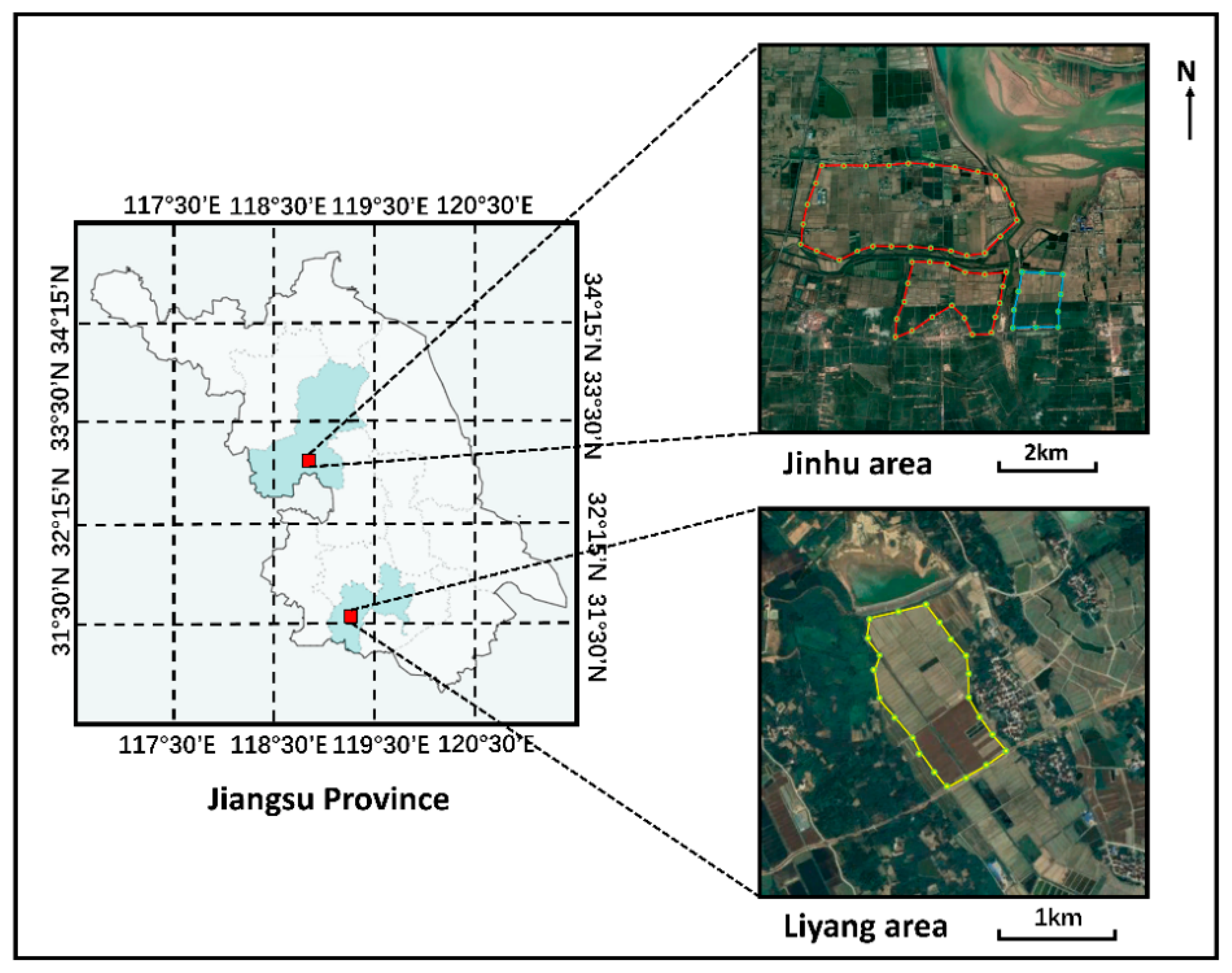
2.1. Study Area
2.2. Ground Data
- Arrange several sampling sites evenly in the rice planting area and use GPS to record their locations.
- The field survey time interval is 3 to 4 days, and the time needs to cover the satellite transit time to guarantee that ground data collecting and radar satellite imaging are synchronized.
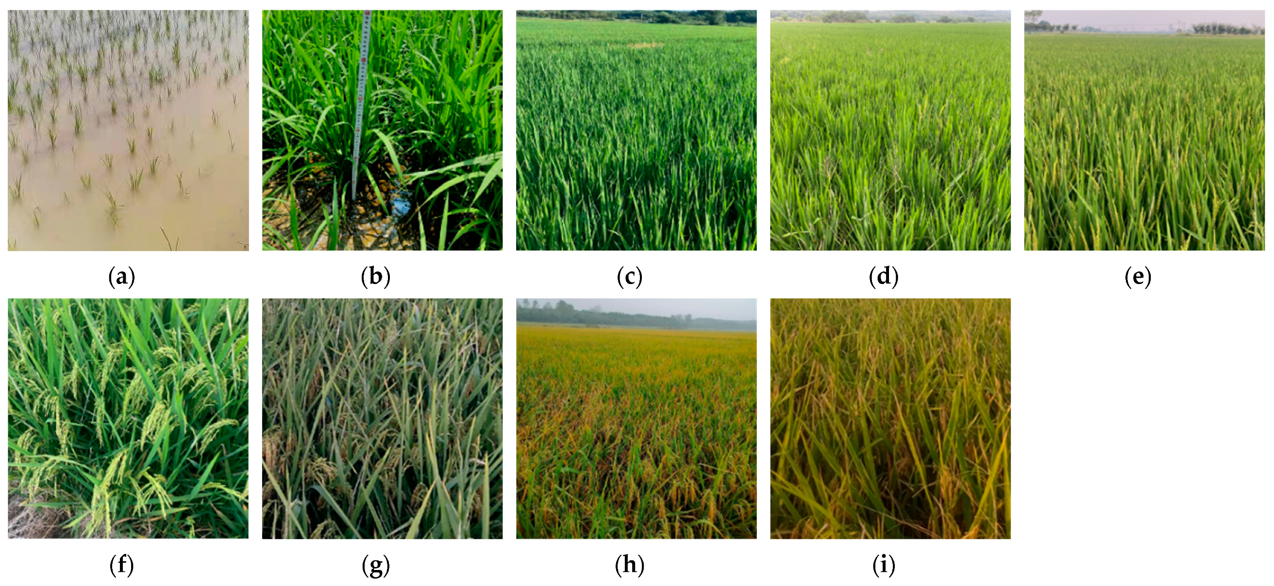
- According to the date of rice planting and the current status of the data acquisition channels, conduct field investigations to collect rice samples and obtain the growth parameters. Collect the ground data of rice samples at the sampling points in the rice-growing area. The contents of the collection include rice species, rice plant height, growth period, planting methods, collection time and weather conditions.
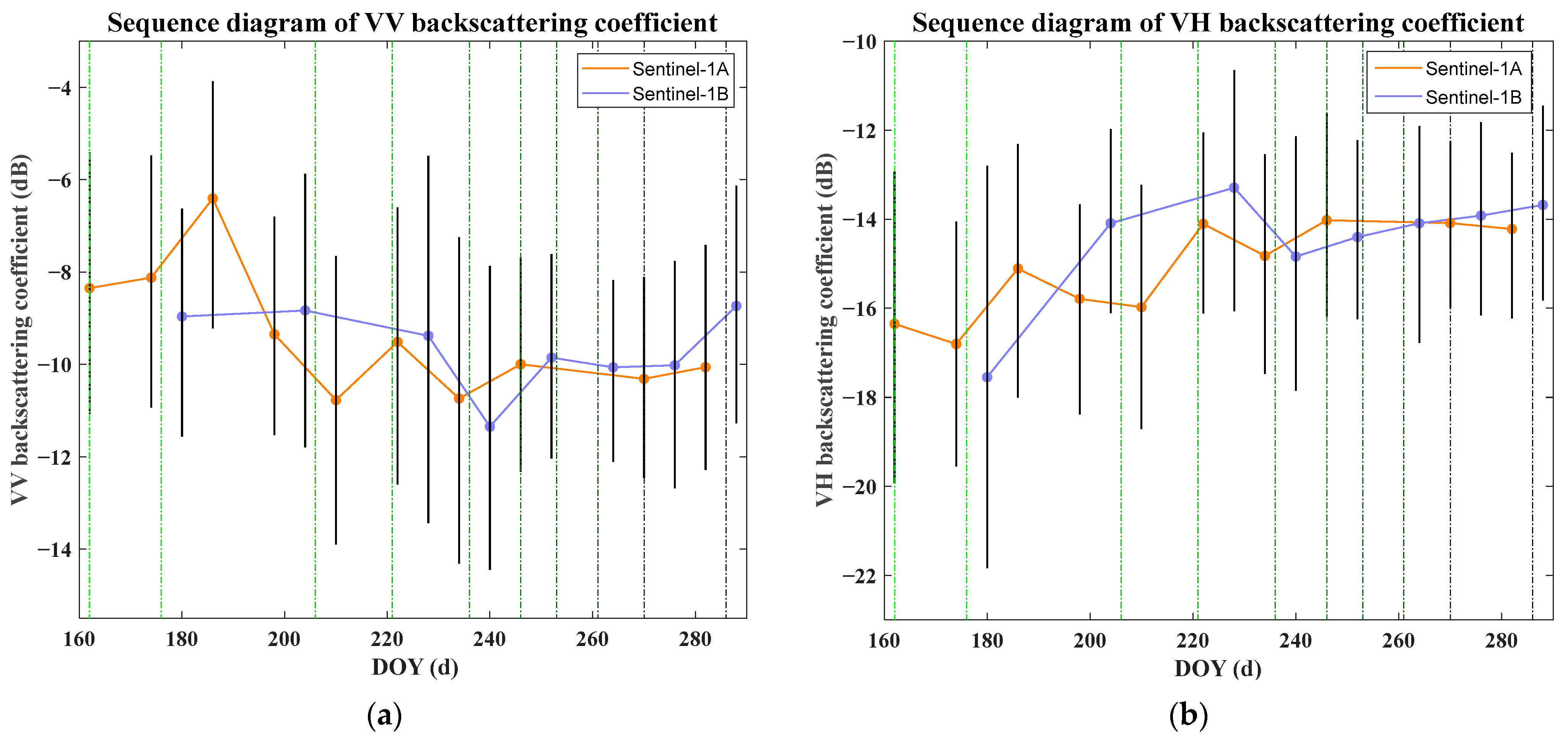
2.3. Sentinel-1 Data
- Multiview processing: average the azimuth or distance of the SLC data to improve the data intensity;
- Speckle filtering: remove the inherent speckle noise of radar images;
- Geocoding and radiometric calibration: combined with the SRTM data of the image coverage area, complete the geocoding and radiometric calibration and extract the backscatter coefficient of the test area in the remote sensing image.
- Calibration: For polarized SAR processing, its radiometric calibration is a complex calibration, which is performed separately for the real and imaginary parts of the complex numbers.
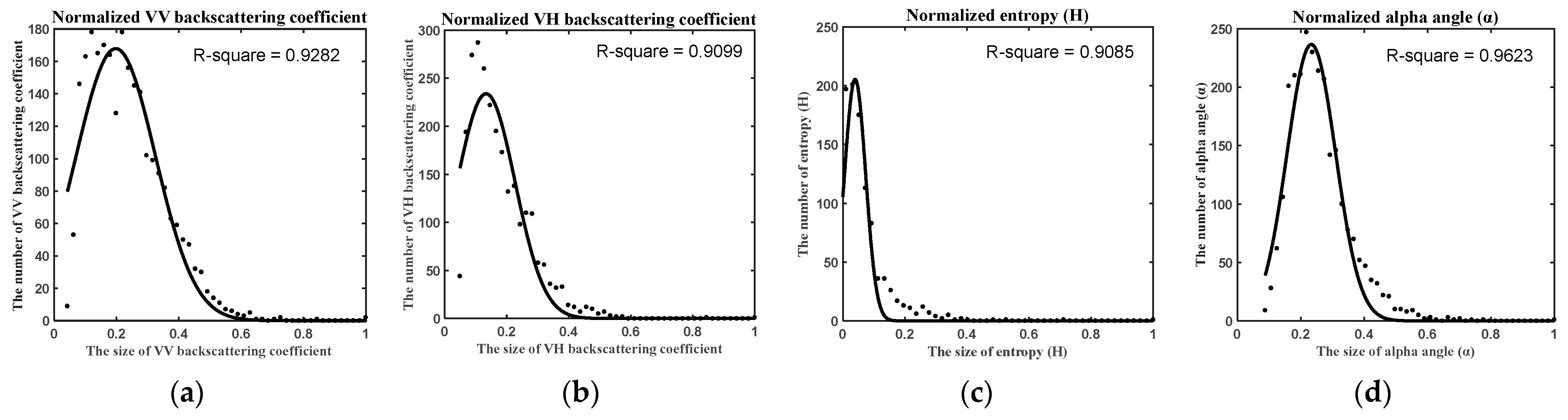
- Polarimetric Metrices: Since the Sentinel-1 satellite has, at most, two polarization channels, only the covariance matrix (C2) can be generated.
- Polarimetric Decomposition: For dual-polarization decomposition, only “H-Alpha Dual Pol Decomposition” can be performed.
3. Methodology
3.1. Rice Growth Curve
3.2. Gaussian Fitting
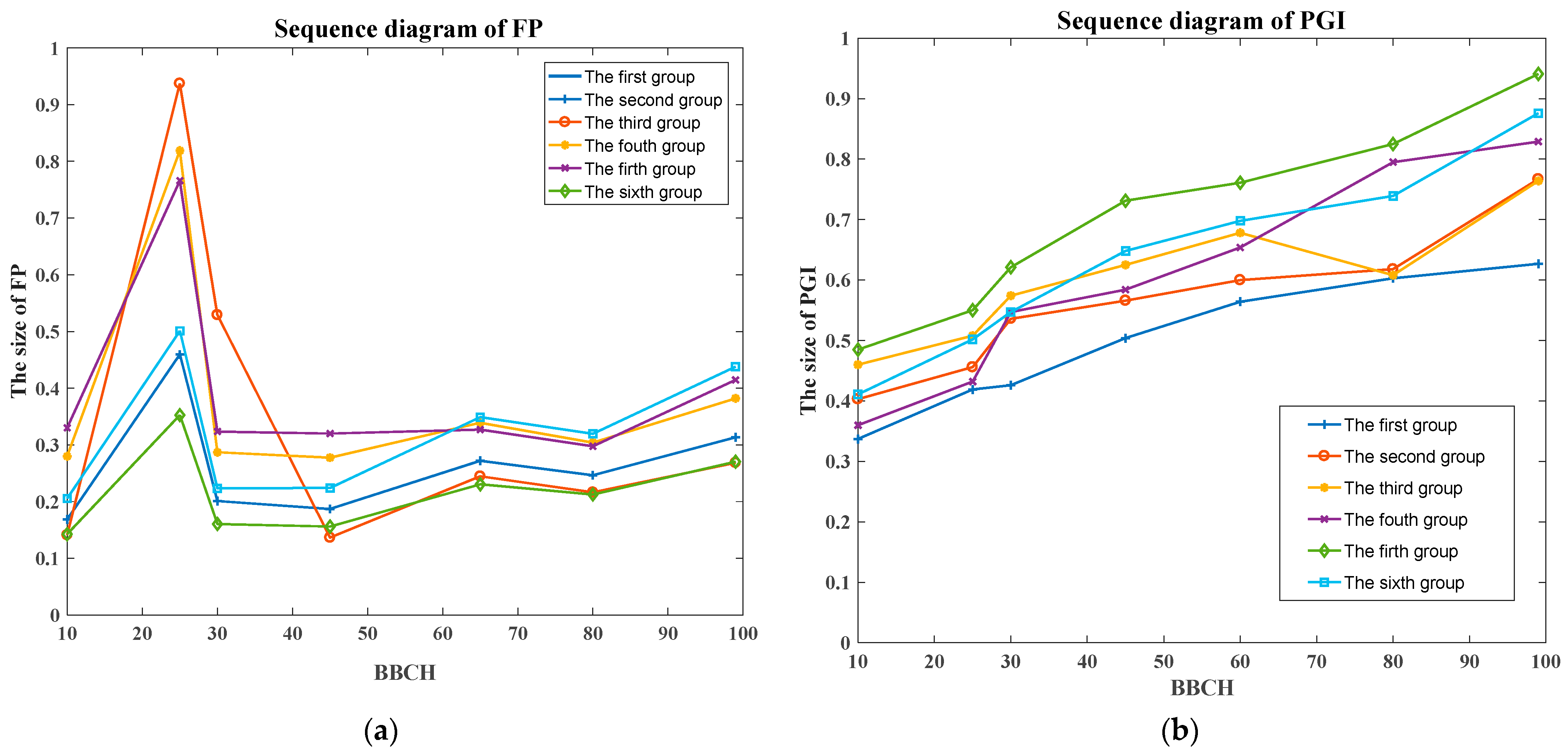
3.3. Data Fusion
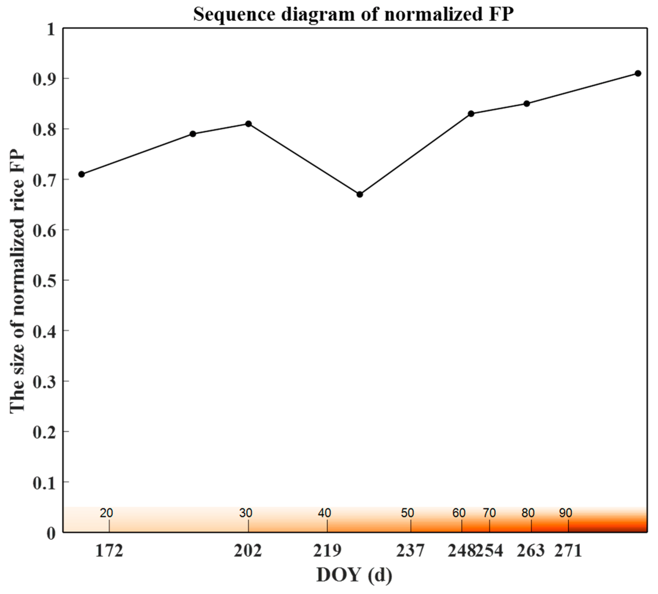
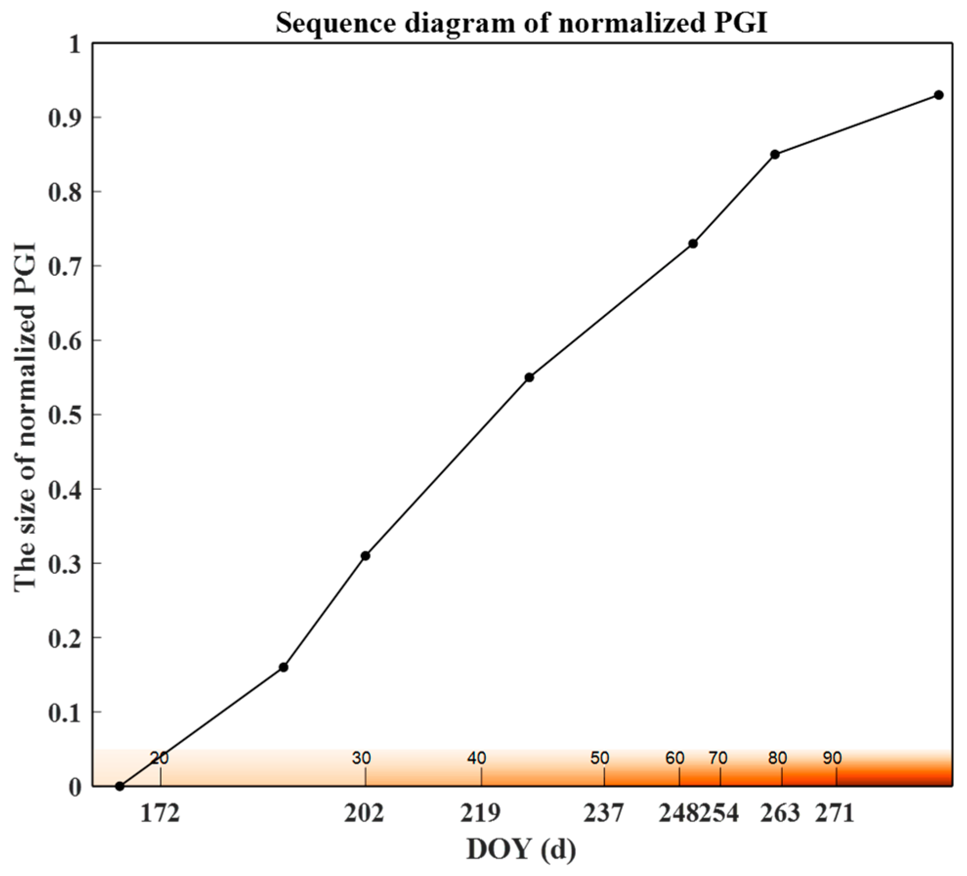
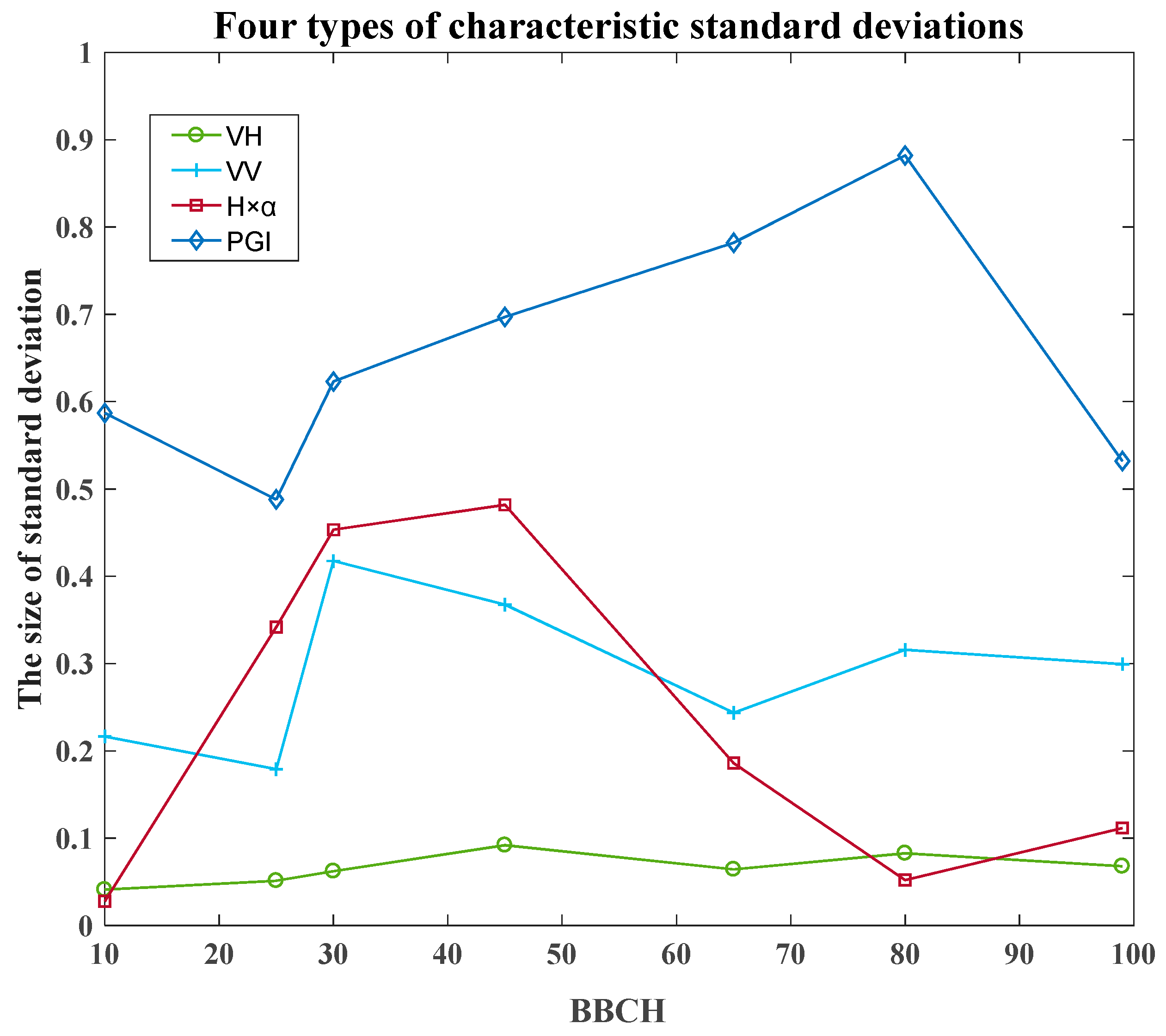
3.4. Polarized Growth Index
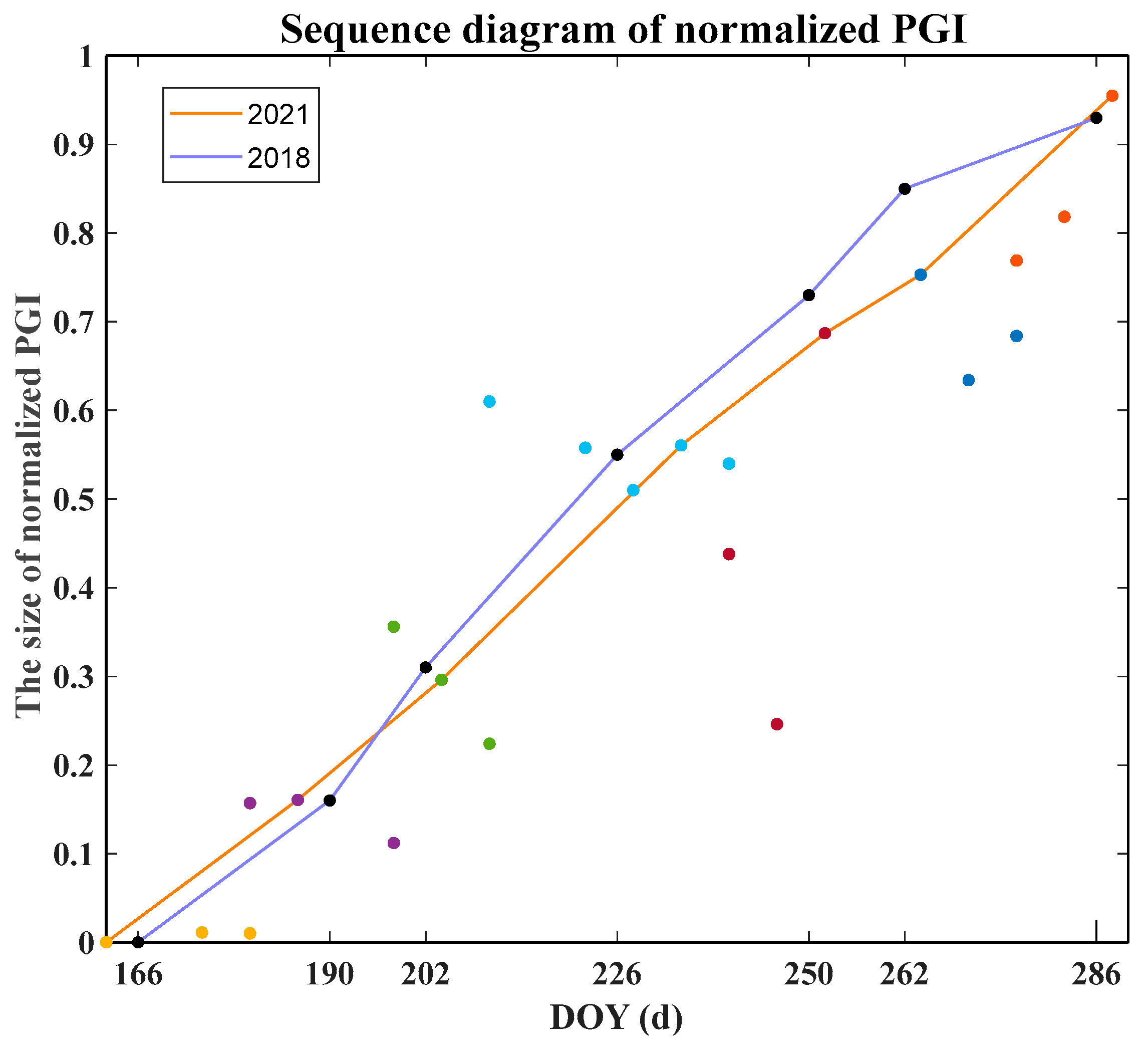
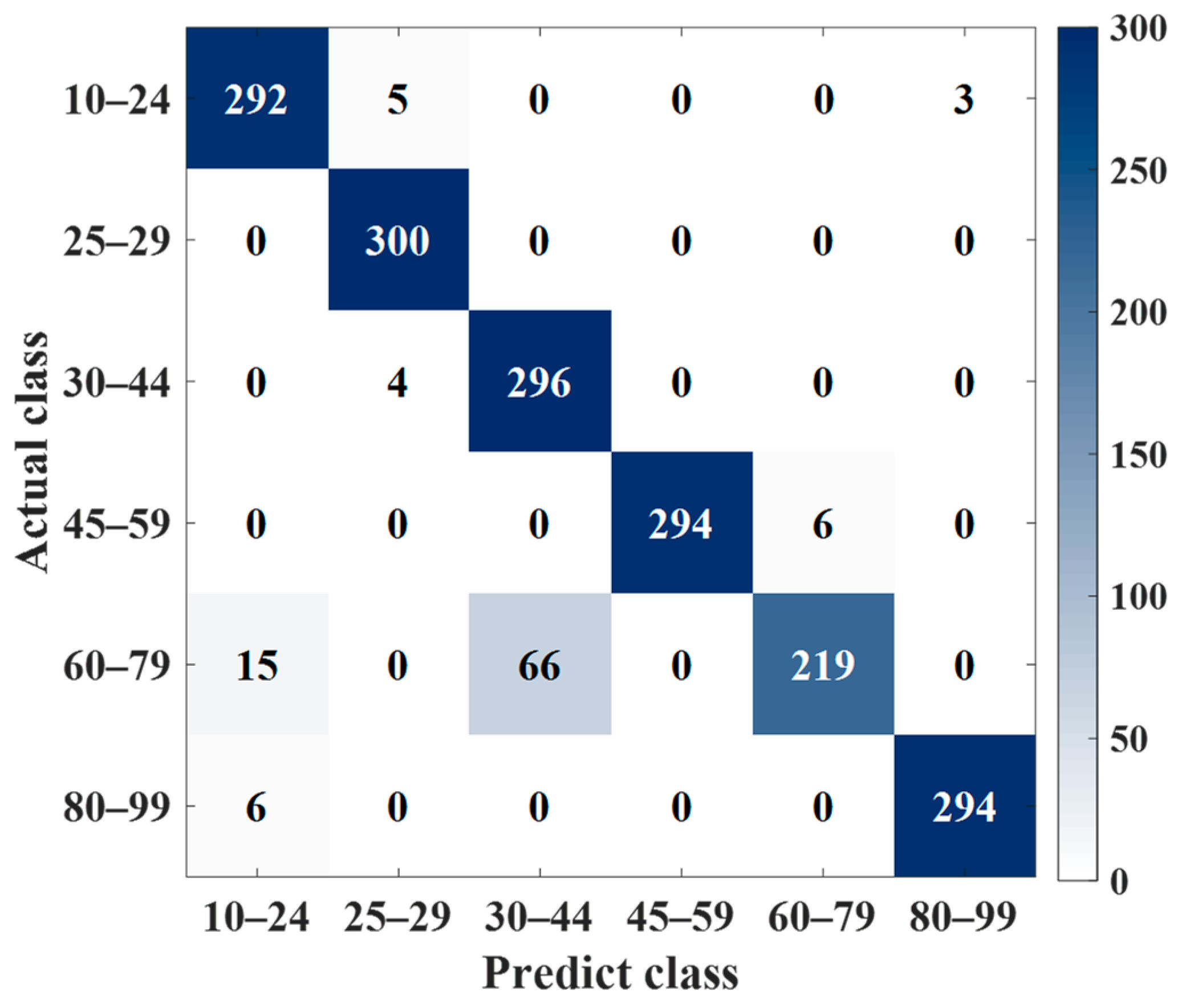
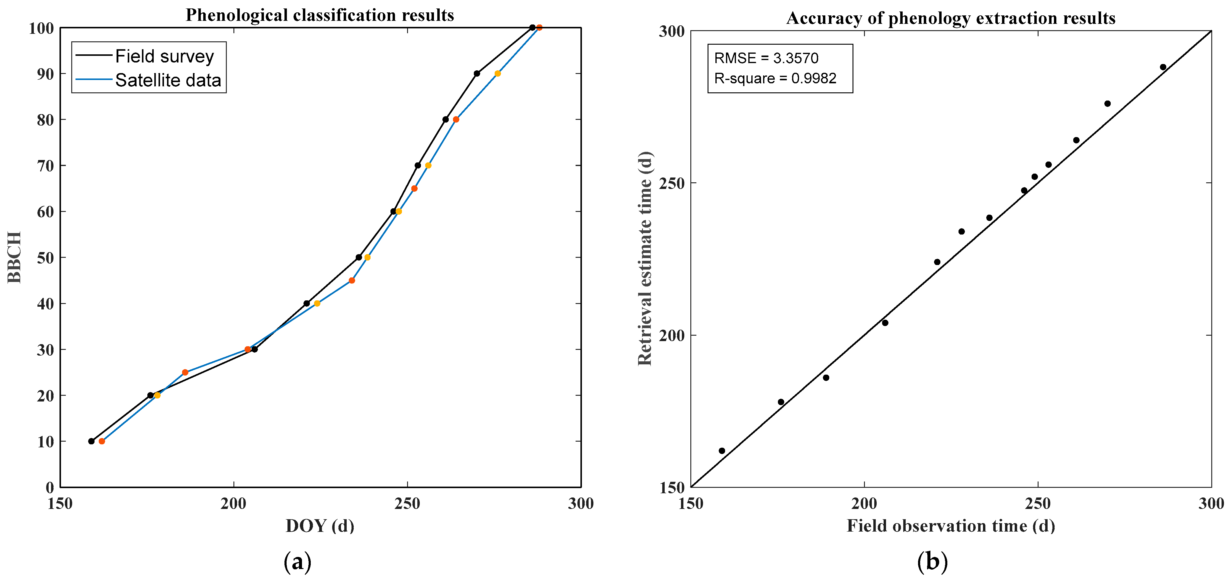
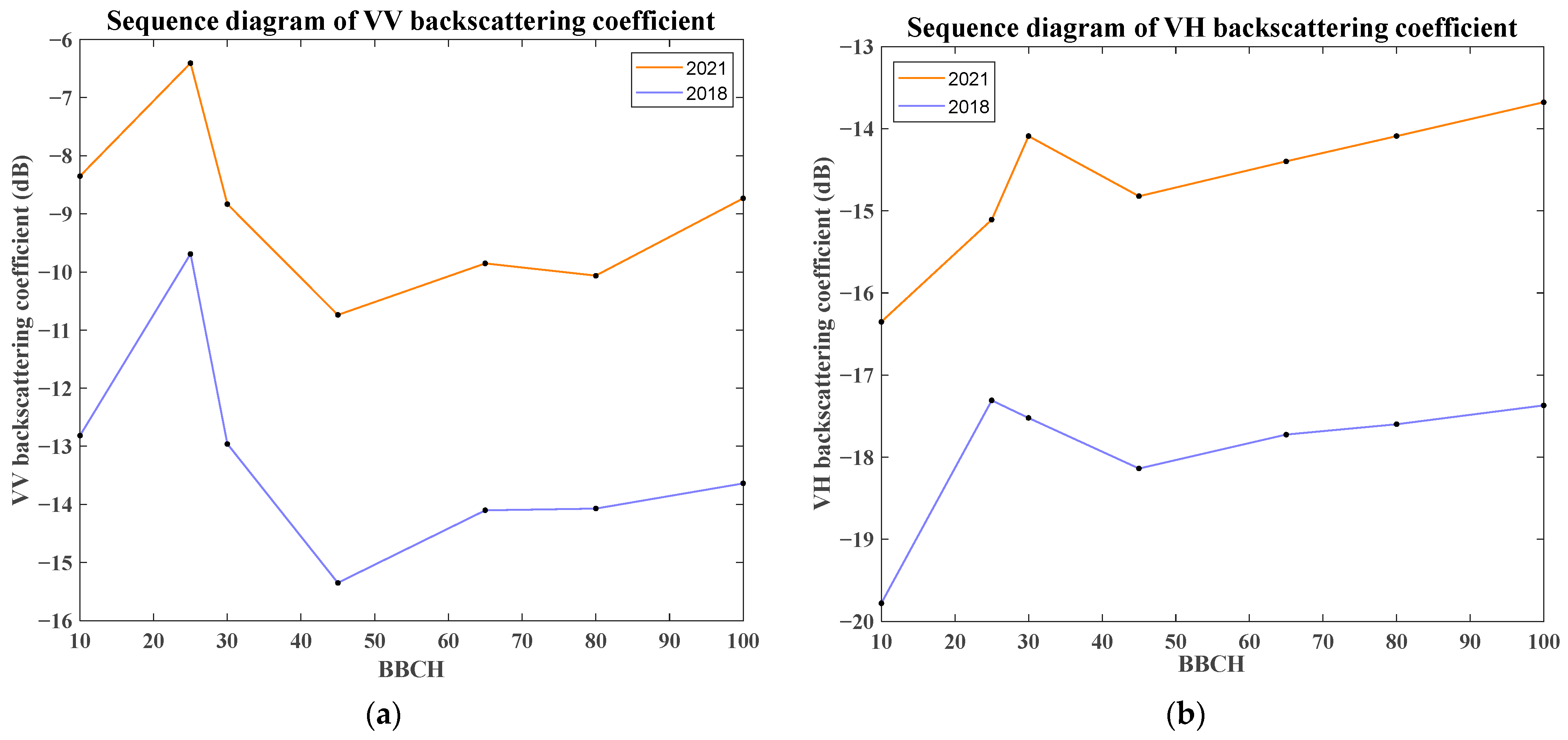
4. Results
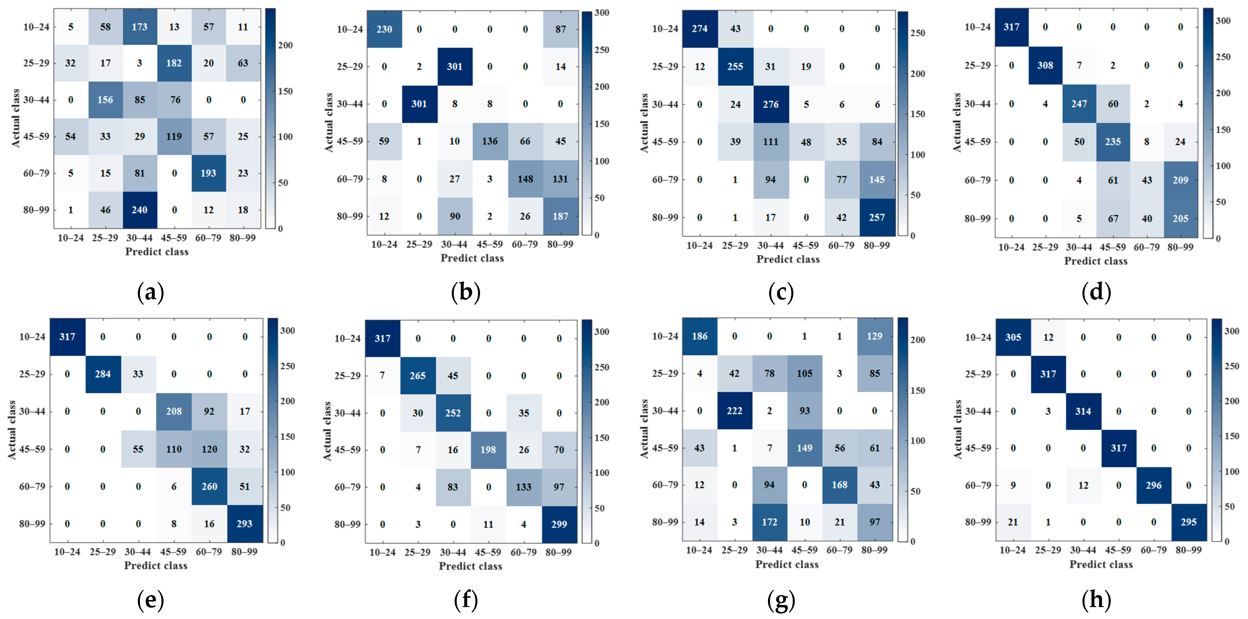
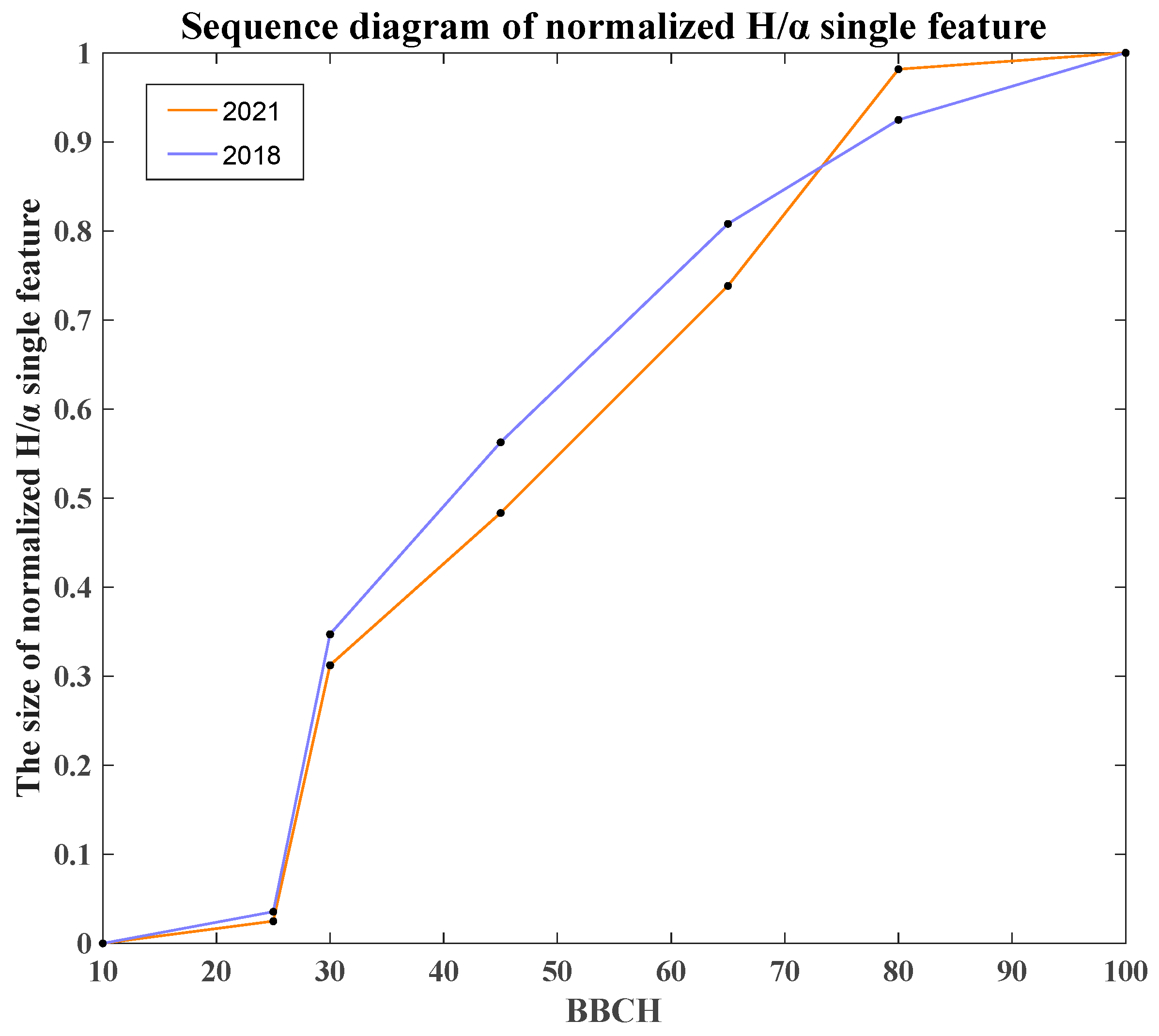
4.1. 2018 Phenology Classification
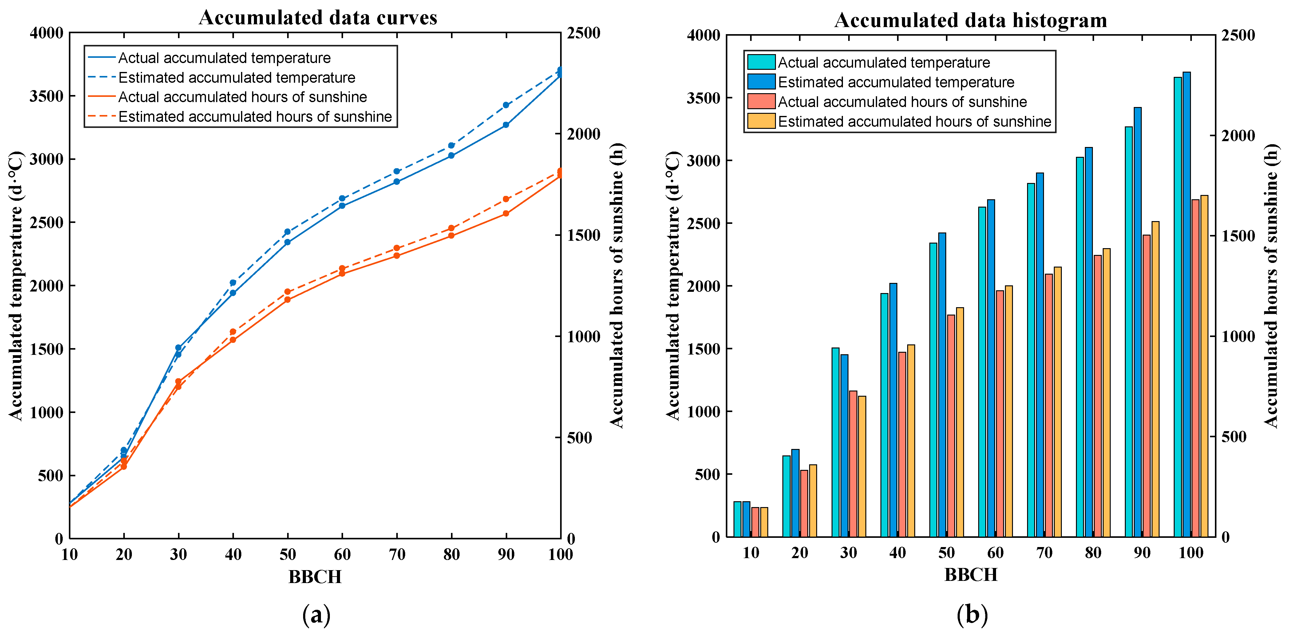
4.2. 2021 Phenology Retrieval
5. Discussion
6. Conclusions
Author Contributions
Funding
Institutional Review Board Statement
Informed Consent Statement
Data Availability Statement
Acknowledgments
Conflicts of Interest
References
- Wang, L.; Wang, Y.; Chen, J. Assessment of the ecological niche of photovoltaic agriculture in China. Sustainability 2019, 11, 2268. [Google Scholar] [CrossRef] [Green Version]
- Chen, J.; Liu, Y.; Wang, L. Research on coupling coordination development for photovoltaic agriculture system in China. Sustainability 2019, 11, 1065. [Google Scholar] [CrossRef] [Green Version]
- Lieth, H. Phenology and Seasonality Modeling; Springer Science & Business Media: Berlin/Heidelberg, Germany, 2013; Volume 8. [Google Scholar]
- Shihua, L.; Jingtao, X.; Ping, N.; Jing, Z.; Hongshu, W.; Jingxian, W. Monitoring paddy rice phenology using time series MODIS data over Jiangxi Province, China. Int. J. Agric. Biol. Eng. 2014, 7, 28–36. [Google Scholar]
- Chen, C.; Son, N.; Chang, L. Monitoring of rice cropping intensity in the upper Mekong Delta, Vietnam using time-series MODIS data. Adv. Space Res. 2012, 49, 292–301. [Google Scholar] [CrossRef]
- Sakamoto, T.; Yokozawa, M.; Toritani, H.; Shibayama, M.; Ishitsuka, N.; Ohno, H. A crop phenology detection method using time-series MODIS data. Remote Sens. Environ. 2005, 96, 366–374. [Google Scholar] [CrossRef]
- Lausch, A.; Salbach, C.; Schmidt, A.; Doktor, D.; Merbach, I.; Pause, M. Deriving phenology of barley with imaging hyperspectral remote sensing. Ecol. Model. 2015, 295, 123–135. [Google Scholar] [CrossRef]
- Yang, Z.; Li, K.; Liu, L.; Shao, Y.; Brisco, B.; Li, W. Rice growth monitoring using simulated compact polarimetric C band SAR. Radio Sci. 2014, 49, 1300–1315. [Google Scholar] [CrossRef]
- Zhang, Y.; Li, L.; Wang, H.; Zhang, Y.; Wang, N.; Chen, J. Land surface phenology of Northeast China during 2000–2015: Temporal changes and relationships with climate changes. Environ. Monit. Assess. 2017, 189, 531. [Google Scholar] [CrossRef]
- Zheng, H.; Cheng, T.; Yao, X.; Deng, X.; Tian, Y.; Cao, W.; Zhu, Y. Detection of rice phenology through time series analysis of ground-based spectral index data. Field Crops Res. 2016, 198, 131–139. [Google Scholar] [CrossRef]
- Richardson, A.D.; Andy Black, T.; Ciais, P.; Delbart, N.; Friedl, M.A.; Gobron, N.; Hollinger, D.Y.; Kutsch, W.L.; Longdoz, B.; Luyssaert, S. Influence of spring and autumn phenological transitions on forest ecosystem productivity. Philos. Trans. R. Soc. B Biol. Sci. 2010, 365, 3227–3246. [Google Scholar] [CrossRef] [Green Version]
- Dash, J.; Jeganathan, C.; Atkinson, P. The use of MERIS Terrestrial Chlorophyll Index to study spatio-temporal variation in vegetation phenology over India. Remote Sens. Environ. 2010, 114, 1388–1402. [Google Scholar] [CrossRef]
- Corcione, V.; Nunziata, F.; Mascolo, L.; Migliaccio, M. A study of the use of COSMO-SkyMed SAR PingPong polarimetric mode for rice growth monitoring. Int. J. Remote Sens. 2016, 37, 633–647. [Google Scholar]
- Peng, D.; Huete, A.R.; Huang, J.; Wang, F.; Sun, H. Detection and estimation of mixed paddy rice cropping patterns with MODIS data. Int. J. Appl. Earth Obs. Geoinf. 2011, 13, 13–23. [Google Scholar] [CrossRef]
- Motohka, T.; Nasahara, K.; Miyata, A.; Mano, M.; Tsuchida, S. Evaluation of optical satellite remote sensing for rice paddy phenology in monsoon Asia using a continuous in situ dataset. Int. J. Remote Sens. 2009, 30, 4343–4357. [Google Scholar] [CrossRef]
- Wang, H.; Chen, J.; Wu, Z.; Lin, H. Rice heading date retrieval based on multi-temporal MODIS data and polynomial fitting. Int. J. Remote Sens. 2012, 33, 1905–1916. [Google Scholar] [CrossRef]
- Zhang, Y.; Liu, X.; Su, S.; Wang, C. Retrieving canopy height and density of paddy rice from Radarsat-2 images with a canopy scattering model. Int. J. Appl. Earth Obs. Geoinf. 2014, 28, 170–180. [Google Scholar]
- He, Z.; Li, S.; Wang, Y.; Dai, L.; Lin, S. Monitoring rice phenology based on backscattering characteristics of multi-temporal RADARSAT-2 datasets. Remote Sens. 2018, 10, 340. [Google Scholar] [CrossRef] [Green Version]
- Lopez-Sanchez, J.M.; Vicente-Guijalba, F.; Ballester-Berman, J.D.; Cloude, S.R. Polarimetric response of rice fields at C-band: Analysis and phenology retrieval. IEEE Trans. Geosci. Remote Sens. 2013, 52, 2977–2993. [Google Scholar] [CrossRef] [Green Version]
- Veloso, A.; Mermoz, S.; Bouvet, A.; Le Toan, T.; Planells, M.; Dejoux, J.-F.; Ceschia, E. Understanding the temporal behavior of crops using Sentinel-1 and Sentinel-2-like data for agricultural applications. Remote Sens. Environ. 2017, 199, 415–426. [Google Scholar] [CrossRef]
- Küçük, Ç.; Taşkın, G.; Erten, E. Paddy-rice phenology classification based on machine-learning methods using multitemporal co-polar X-band SAR images. IEEE J. Sel. Top. Appl. Earth Obs. Remote Sens. 2016, 9, 2509–2519. [Google Scholar] [CrossRef]
- Wang, H.; Magagi, R.; Goïta, K.; Trudel, M.; McNairn, H.; Powers, J. Crop phenology retrieval via polarimetric SAR decomposition and Random Forest algorithm. Remote Sens. Environ. 2019, 231, 111234. [Google Scholar] [CrossRef]
- Mascolo, L.; Lopez-Sanchez, J.M.; Vicente-Guijalba, F.; Nunziata, F.; Migliaccio, M.; Mazzarella, G. A complete procedure for crop phenology estimation with PolSAR data based on the complex Wishart classifier. IEEE Trans. Geosci. Remote Sens. 2016, 54, 6505–6515. [Google Scholar] [CrossRef] [Green Version]
- Balenzano, A.; Mattia, F.; Satalino, G.; Davidson, M.W. Dense temporal series of C-and L-band SAR data for soil moisture retrieval over agricultural crops. IEEE J. Sel. Top. Appl. Earth Obs. Remote Sens. 2010, 4, 439–450. [Google Scholar] [CrossRef]
- Mattia, F.; Le Toan, T.; Picard, G.; Posa, F.I.; D’Alessio, A.; Notarnicola, C.; Gatti, A.M.; Rinaldi, M.; Satalino, G.; Pasquariello, G. Multitemporal C-band radar measurements on wheat fields. IEEE Trans. Geosci. Remote Sens. 2003, 41, 1551–1560. [Google Scholar] [CrossRef]
- Skriver, H.; Svendsen, M.T.; Thomsen, A.G. Multitemporal C-and L-band polarimetric signatures of crops. IEEE Trans. Geosci. Remote Sens. 1999, 37, 2413–2429. [Google Scholar] [CrossRef]
- Kussul, N.; Lemoine, G.; Gallego, F.J.; Skakun, S.V.; Lavreniuk, M.; Shelestov, A.Y. Parcel-based crop classification in Ukraine using Landsat-8 data and Sentinel-1A data. IEEE J. Sel. Top. Appl. Earth Obs. Remote Sens. 2016, 9, 2500–2508. [Google Scholar] [CrossRef]
- Lasko, K.; Vadrevu, K.P.; Tran, V.T.; Justice, C. Mapping double and single crop paddy rice with Sentinel-1A at varying spatial scales and polarizations in Hanoi, Vietnam. IEEE J. Sel. Top. Appl. Earth Obs. Remote Sens. 2018, 11, 498–512. [Google Scholar] [CrossRef] [PubMed]
- De Bernardis, C.G.; Vicente-Guijalba, F.; Martinez-Marin, T.; Lopez-Sanchez, J.M. Estimation of key dates and stages in rice crops using dual-polarization SAR time series and a particle filtering approach. IEEE J. Sel. Top. Appl. Earth Obs. Remote Sens. 2014, 8, 1008–1018. [Google Scholar] [CrossRef] [Green Version]
- Nelson, A.; Setiyono, T.; Rala, A.B.; Quicho, E.D.; Raviz, J.V.; Abonete, P.J.; Maunahan, A.A.; Garcia, C.A.; Bhatti, H.Z.M.; Villano, L.S. Towards an operational SAR-based rice monitoring system in Asia: Examples from 13 demonstration sites across Asia in the RIICE project. Remote Sens. 2014, 6, 10773–10812. [Google Scholar] [CrossRef] [Green Version]
- Kumar, P.; Prasad, R.; Gupta, D.; Mishra, V.; Vishwakarma, A.; Yadav, V.; Bala, R.; Choudhary, A.; Avtar, R. Estimation of winter wheat crop growth parameters using time series Sentinel-1A SAR data. Geocarto Int. 2018, 33, 942–956. [Google Scholar] [CrossRef]
- Fikriyah, V.N.; Darvishzadeh, R.; Laborte, A.; Khan, N.I.; Nelson, A. Discriminating transplanted and direct seeded rice using Sentinel-1 intensity data. Int. J. Appl. Earth Obs. Geoinf. 2019, 76, 143–153. [Google Scholar] [CrossRef] [Green Version]
- Arias, M.; Campo-Bescós, M.Á.; Álvarez-Mozos, J. Crop classification based on temporal signatures of Sentinel-1 observations over Navarre province, Spain. Remote Sens. 2020, 12, 278. [Google Scholar] [CrossRef] [Green Version]
- Canisius, F.; Shang, J.; Liu, J.; Huang, X.; Ma, B.; Jiao, X.; Geng, X.; Kovacs, J.M.; Walters, D. Tracking crop phenological development using multi-temporal polarimetric Radarsat-2 data. Remote Sens. Environ. 2018, 210, 508–518. [Google Scholar] [CrossRef]
- Khabbazan, S.; Vermunt, P.; Steele-Dunne, S.; Ratering Arntz, L.; Marinetti, C.; van der Valk, D.; Iannini, L.; Molijn, R.; Westerdijk, K.; van der Sande, C. Crop monitoring using Sentinel-1 data: A case study from The Netherlands. Remote Sens. 2019, 11, 1887. [Google Scholar] [CrossRef] [Green Version]
- Yang, H.; Pan, B.; Wu, W.; Tai, J. Field-based rice classification in Wuhua county through integration of multi-temporal Sentinel-1A and Landsat-8 OLI data. Int. J. Appl. Earth Obs. Geoinf. 2018, 69, 226–236. [Google Scholar] [CrossRef]
- Vicente-Guijalba, F.; Martinez-Marin, T.; Lopez-Sanchez, J.M. Dynamical approach for real-time monitoring of agricultural crops. IEEE Trans. Geosci. Remote Sens. 2014, 53, 3278–3293. [Google Scholar] [CrossRef] [Green Version]
- Lopez-Sanchez, J.M.; Cloude, S.R.; Ballester-Berman, J.D. Rice phenology monitoring by means of SAR polarimetry at X-band. IEEE Trans. Geosci. Remote Sens. 2011, 50, 2695–2709. [Google Scholar] [CrossRef]
- Lancashire, P.D.; Bleiholder, H.; Boom, T.V.D.; Langelüddeke, P.; Stauss, R.; Weber, E.; Witzenberger, A. A uniform decimal code for growth stages of crops and weeds. Ann. Appl. Biol. 1991, 119, 561–601. [Google Scholar] [CrossRef]
- McMartin, A. The logistic curve of plant growth and its application to sugarcane. Proc. S. Afr. Sugar Technol. Assoc. 1979, 53, 189–193. [Google Scholar]
- Lopez-Sanchez, J.M.; Ballester-Berman, J.D.; Hajnsek, I. First results of rice monitoring practices in Spain by means of time series of TerraSAR-X dual-pol images. IEEE J. Sel. Top. Appl. Earth Obs. Remote Sens. 2010, 4, 412–422. [Google Scholar] [CrossRef]
- Attema, E.; Ulaby, F.T. Vegetation modeled as a water cloud. Radio Sci. 1978, 13, 357–364. [Google Scholar] [CrossRef]
- Guo, J.; Wei, P.-L.; Liu, J.; Jin, B.; Su, B.-F.; Zhou, Z.-S. Crop Classification Based on Differential Characteristics of H/α Scattering Parameters for Multitemporal Quad-and Dual-Polarization SAR Images. IEEE Trans. Geosci. Remote Sens. 2018, 56, 6111–6123. [Google Scholar] [CrossRef]
- Greff, K.; Srivastava, R.K.; Koutník, J.; Steunebrink, B.R.; Schmidhuber, J. LSTM: A search space odyssey. IEEE Trans. Neural Netw. Learn. Syst. 2016, 28, 2222–2232. [Google Scholar] [CrossRef] [PubMed] [Green Version]
- Rost, S.; Gerten, D.; Hoff, H.; Lucht, W.; Falkenmark, M.; Rockström, J. Global potential to increase crop production through water management in rainfed agriculture. Environ. Res. Lett. 2009, 4, 044002. [Google Scholar] [CrossRef]
- Challinor, A.J.; Simelton, E.S.; Fraser, E.D.; Hemming, D.; Collins, M. Increased crop failure due to climate change: Assessing adaptation options using models and socio-economic data for wheat in China. Environ. Res. Lett. 2010, 5, 034012. [Google Scholar] [CrossRef]
- Tester, M.; Langridge, P. Breeding technologies to increase crop production in a changing world. Science 2010, 327, 818–822. [Google Scholar] [CrossRef]


| Major Stage | BBCH Scale | Description |
|---|---|---|
| Vegetative | 00–09 | Germination |
| 10–19 | Leaf development | |
| 20–29 | Tillering | |
| 30–39 | Stem elongation | |
| Reproductive | 40–49 | Booting |
| 50–59 | Inflorescence emergence | |
| 60–69 | Flowering, anthesis | |
| Ripening | 70–79 | Development of fruit |
| 80–89 | Ripening | |
| 90–99 | Senescence |
| Satellite | Sentinel-1 |
|---|---|
| Swath width | 250 km |
| Revisit period | 12 d or 6 d |
| Spatial resolution | 5 m × 20 m |
| Relative orbit number | 69 |
| Acquisition date | 15 June 2018 to 13 October 2018; 11 June 2021 to 15 October 2021 |
| Incident angles | 32–34°; 38–40° |
| Polarization scheme | VH, VV |
| Class | 0–24 | 25–29 | 30–44 | 45–64 | 65–79 | 80–99 | Total |
|---|---|---|---|---|---|---|---|
| LSTMVH | 1.57% | 5.36% | 26.81% | 37.54% | 60.88% | 5.68% | 22.97% |
| LSTMVV | 72.56% | 0.63% | 2.52% | 42.90% | 46.69% | 58.99% | 37.38% |
| LSTMH/α | 86.43% | 80.44% | 87.07% | 15.14% | 24.29% | 81.07% | 62.41% |
| LSTMFP | 58.68% | 13.25% | 0.63% | 47.00% | 53.00% | 30.60% | 33.86% |
| LSTMVH_GC | 100% | 97.16% | 77.92% | 74.13% | 13.56% | 64.67% | 71.24% |
| LSTMVV_GC | 100% | 89.59% | 0% | 34.70% | 82.01% | 92.43% | 66.46% |
| LSTMH/α_GC | 100% | 83.60% | 79.50% | 62.46% | 41.96% | 94.32% | 76.97% |
| LSTMPGI | 96.21% | 100% | 99.05% | 100% | 93.38% | 93.06% | 96.95% |
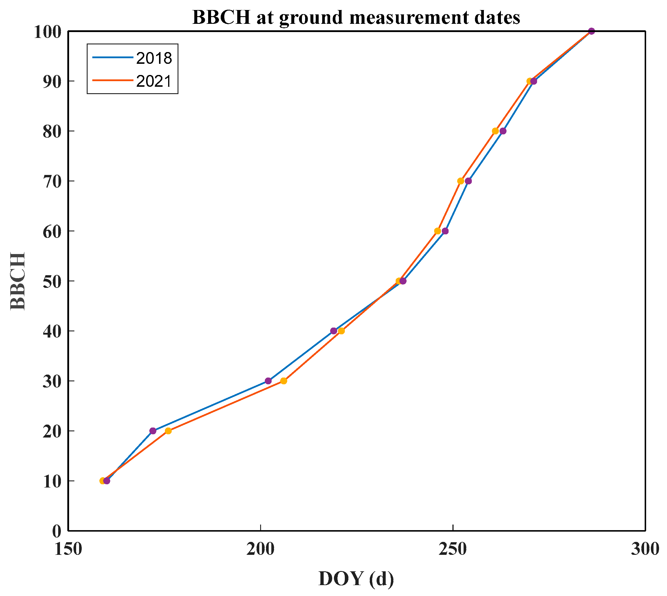
| BBCH | Field Observation Time/d | Retrieval Estimate Time/d | Error/d |
|---|---|---|---|
| 10 | 159 | 162 | 3 |
| 20 | 176 | 178 | 2 |
| 25 | 189 | 186 | 3 |
| 30 | 206 | 204 | 2 |
| 40 | 221 | 224 | 3 |
| 45 | 228 | 234 | 6 |
| 50 | 236 | 238.5 | 2.5 |
| 60 | 246 | 247.5 | 1.5 |
| 65 | 249 | 252 | 3 |
| 70 | 253 | 256 | 3 |
| 80 | 261 | 264 | 3 |
| 90 | 270 | 276 | 6 |
| 100 | 286 | 288 | 2 |
| Total | 3.08 | ||
Publisher’s Note: MDPI stays neutral with regard to jurisdictional claims in published maps and institutional affiliations. |
© 2022 by the authors. Licensee MDPI, Basel, Switzerland. This article is an open access article distributed under the terms and conditions of the Creative Commons Attribution (CC BY) license (https://creativecommons.org/licenses/by/4.0/).
Share and Cite
Wang, B.; Liu, Y.; Sheng, Q.; Li, J.; Tao, J.; Yan, Z. Rice Phenology Retrieval Based on Growth Curve Simulation and Multi-Temporal Sentinel-1 Data. Sustainability 2022, 14, 8009. https://doi.org/10.3390/su14138009
Wang B, Liu Y, Sheng Q, Li J, Tao J, Yan Z. Rice Phenology Retrieval Based on Growth Curve Simulation and Multi-Temporal Sentinel-1 Data. Sustainability. 2022; 14(13):8009. https://doi.org/10.3390/su14138009
Chicago/Turabian StyleWang, Bo, Yu Liu, Qinghong Sheng, Jun Li, Jiahui Tao, and Zhijun Yan. 2022. "Rice Phenology Retrieval Based on Growth Curve Simulation and Multi-Temporal Sentinel-1 Data" Sustainability 14, no. 13: 8009. https://doi.org/10.3390/su14138009
APA StyleWang, B., Liu, Y., Sheng, Q., Li, J., Tao, J., & Yan, Z. (2022). Rice Phenology Retrieval Based on Growth Curve Simulation and Multi-Temporal Sentinel-1 Data. Sustainability, 14(13), 8009. https://doi.org/10.3390/su14138009