Abstract
The purpose of this work was to develop a problem-solving approach and a simulation tool that is useful for the specification of wastewater treatment process equipment design parameters. The proposition of using an artificial neural network (ANN) numerical model for supervised learning of a dataset and then for process simulation on a new dataset was investigated. The effectiveness of the approach was assessed by evaluating the capacity of the model to distinguish differences in the equipment design parameters. To demonstrate the approach, a mock dataset was derived from experimentally acquired data and physical effects reported in the literature. The mock dataset comprised the influent flow rate, the bed packing material dimension, the type of packing material and the packed bed height-to-diameter ratio as predictors of the calorific value reduction. The multilayer perceptron (MLP) ANN was compared to a polynomial model. The validation test results show that the MLP model has four hidden layers, each having 256 units (nodes), accurately predicts calorific value reduction. When the model was fed previously unseen test data, the root-mean-square error (RMSE) of the predicted responses was 0.101 and the coefficient of determination (R2) was 0.66. The results of simulation of all 125 possible combinations of the 3 mechanical parameters and identical influent wastewater flow profiles were ranked according to total calorific value reduction. A t-test of the difference between the mean calorific value reduction of the two highest ranked experiments showed that the means are significantly different (p-value = 0.011). Thus, the model has the capacity to distinguish differences in the equipment design parameters. Consequently, the values of the three mechanical feature parameters from the highest ranked simulated experiment are recommended for use in the design of the industrial scale upflow anaerobic filter (UAF) for wastewater treatment.
1. Introduction
Bioprocesses are defined as controlled conditions that result in the biological agent-mediated transformation of a substrate chemical into a specific product chemical. Wastewater treatment processes are environmental bioprocesses designed to improve environmental quality. They are often designed, simulated, and optimized using the conventional International Water Association (IWA) approach to modeling the wastewater treatment process implemented as differential and algebraic equations [1]. Process specification includes the evaluation of the physical and chemical parameters of the feed and product streams and of the internal biochemical and physical-chemical process steps. Initial bioprocess development is typically conducted in small laboratory bioreactors (between 1 and 10 L working volume) of standard mechanical configurations using defined synthetic substrates under highly controlled conditions. Factorial designed experiments with polynomial regression analysis and hybrid (discrete/continuous) systems approaches are used to determine the significant parameters and the operating set points [2,3,4].
This conventional approach might not adequately account for the variation encountered under real industrial, and especially under real environmental conditions where it is not possible to continuously measure and regulate the substrate composition and mass flow [5,6]. In a review of the hydrodynamic models of anaerobic bioreactors, Liotta et al. [7], presented and compared the conventional numeric mathematical approaches including plug flow, tank in series, dispersion and computational fluid dynamic models. This review noted that model calibration often aims to assess key hydrodynamic parameters using tracer tests and that the kinetic constants are assessed if the biochemical modules are implemented. It was also noted that there are few attempts to apply the models for the optimum design and scale-up of bioreactors. Thus, a more comprehensive and integrated approach is needed.
Bioprocesses involve complex interactions between the temperature, liquid flow parameters, substrates and a dynamic community of microbes that are difficult to specify, model and control [8,9]. Additionally, the mechanical characteristics and constructive features of the full-scale bioreactor can be very different from those at the laboratory scale. To address these issues, many researchers have recognized the usefulness to shift towards a “black-box” approach for modeling environmental bioprocesses and engineered systems. Instead of attempting to characterize biochemical reaction mechanisms, a “black-box” approach aims to build a robust model of the process based on easily measurable system parameters such as influent flow rate, product flow, vessel dimensions and constructive features, and operating set-points [10,11]. This approach does not require the determination of bioprocess parameters such as feed and product stream composition, fluid flow parameters, kinetic coefficients, inhibition factors and the identity of the active microbes, but requires a large dataset that covers a wide range of operating conditions.
Artificial neural network (ANN) models are “black-box” models. They are calculation tools, rather than precise descriptions of chemical reaction mechanisms and physical reactors. ANNs have demonstrated their capacity to map complex and non-linear relations between data [12,13,14] with applications to environmental bioprocesses [15,16,17,18]. For example, an ANN model of empirical data has been developed to investigate the optimum conditions for formaldehyde removal from air by a bio trickling filter [19]. The authors used the model to assess removal efficiency as a function of operating conditions and sensitivity analysis was used to determine the relative contribution of each input parameter to the outputs. In another study, a multilayer perceptron (MLP) model was developed to simulate and predict sprinkler precipitation from the input parameters of operating pressure, wind speed, wind direction and sprinkler nozzle diameter with the goal of reducing the time and cost of determining sprinkler irrigation uniformity coefficients [20]. To optimize the hydrodynamic parameters on inverse fluidized bed reactors, an MLP model was also trained using the same data organized in the same Box–Behnken experimental plan as was used to make a model based on the response surface methodology (RSM) [21]. This study found that the ANN model more accurately predicted dependent variables whereas both the RSM and the ANN models were helpful in optimization. Moving in the same direction, another study used a macroscopic, black-box approach to overcome the difficulty in modeling a hybrid and multivariate filtration process [22]. The authors successfully approximated the breakthrough curves using an ANN model using operational parameters (i.e., feed flow rate, initial concentration, adsorption bed length and filter sheet type) as predictors, and easily measurable objective variables to evaluate the process performance. In another study, correlation analysis and decomposition of the time series were used to identify the most important process parameters [23]. The authors then built an ANN-based intelligent system to predict effluent COD from the important process parameters. The model achieved a prediction accuracy (MAPE) of 10.8%.
Anaerobic contact processes for domestic sewage treatment were first described in the mid-20th century [24,25,26]. In this framework, an upflow anaerobic filter (UAF) bioreactor was proposed [27,28,29,30]. The UAF is type of fixed bed bioreactor comprised of a vessel that contains a packed bed of solid supports (packing) on which a strongly attached biofilm develops [31]. Influent wastewater enters below the bed, flows upwards, comes into contact with the biofilm and then exits the vessel from an outlet located above the bed. The biofilm is composed of a community of microorganisms which are the functional agents of the biotransformation of substrate to product. By a process known as anaerobic digestion, some components of the wastewater are transformed into biogas that exits the system, thereby reducing the water pollution. The advantage of the design is the dense, fixed film community of bacteria that tolerates variations in influent stream flow rate and quality, thus making it possible to reduce the vessel volume and to treat influent wastewater, whose characteristics such as chemical composition, temperature and flow rate vary over a wide range.
Evidently, the use of machine learning techniques is common in the field of wastewater treatment process modeling. Among machine learning techniques, it was recently reported that ANNs comprised 65% of the models used in WWTP process forecasting [23]. The majority of studies focused on wastewater treatment plant operational parameters that predict effluent quality. The models were mainly used for fault detection and operations forecasting. Very few studies have focused on mechanical design parameters as predictors of effluent quality. In this context, the present study is different because the model predictors are the mechanical features of the process equipment, and additionally, the model can be used to simulate different mechanical feature values during the equipment design process. To develop high-performance environmental bioprocesses, what is needed is a simulation tool that is capable of accounting for many complex and varying hydraulic and biological system parameters, variations over daily or even seasonal time periods, variable process control parameters, fixed mechanical constructive parameters and the non-linear and temporal relations between them [5,11,32]. Hence, a method for non-linear system identification and for fixed mechanical parameter estimation is required. This study aimed to develop a method to meet these requirements in the context of designing a fixed bed bioreactor.
The present work is a proof of concept study. The method and original workflow presented herein are intended to improve the entire environmental bioprocess development workflow from raw data collection to design specification. This study tests the hypothesis that an artificial neural network model can be used to distinguish different sets of upflow anaerobic filter mechanical set-point values by simulation. The experimental plan and the method to build and use the artificial neural network model are presented and discussed. Thus, the specific objectives of this study are to demonstrate and evaluate:
- An efficient experimental plan that can be implemented in field conditions;
- The accuracy of the artificial neural network predictive model;
- The selection of mechanical constructive parameters based on significant differences in the performance results obtained by simulation.
2. Materials and Methods
2.1. Problem Solving Approach
The approach to solving the problem consists of the following steps:
- Installation of a bioreactor testing and data acquisition system at an industrial site;
- Preparation of an experimental plan to vary the operational parameters such that the test system is exposed to the full range of possible industrial conditions;
- Operation of the test system according to the experimental plan to acquire raw data;
- Restructuring and pre-treatment of the raw dataset according to the requirements of ANN models and to describe individual experiments according to the experimental plan;
- Construction of an artificial neural network model;
- Training and validation of the ANN model using supervised learning;
- Use of the ANN model to simulate test cases where mechanical parameters are varied within the range of tested values;
- Ranking of the simulation results in terms of the predicted performance of the upflow anaerobic filter bioreactor;
- Selection of the mechanical parameters according to the ranking of the simulation results.
2.2. Direct Experimental Data
The test unit used in this study was a purpose-built cylindrical, unheated, fixed bed bioreactor having a vessel liquid volume of 37 L (). The test unit was installed at a municipal wastewater treatment plant located in Yverdon-les-Bains, Switzerland, and was continuously fed raw primary sedimentation basin overflow using a peristaltic pump set to deliver wastewater at a specified flow rate between 127 and 516 L·day. Three major mechanical factors were considered to affect the bioprocess: the packing equivalent spherical diameter (), the packing material type (), and the fixed bed height/diameter ratio (). More than 95% of the packing material used was torrefied wood chips (TWD) with low sphericity ( mm). In order to evaluate other packing materials, the remaining 5% was composed of a mixture of polyvinyl chloride (PVC) chips, polyethylene tubes, polyurethane foam (PUF) cubes, ceramic and glass chips placed throughout the fixed bed. The relative biofilm activity of each type of material was determined by the dehydrogenase enzyme activity tests [33] of packing material samples removed from the bioreactor during the experiments. The fixed bed height/diameter ratio of our experimental bioreactor was 1.8 ().
Data were collected during continuous operation under industrial conditions from 4 May until 12 December 2017. The water temperature (inlet, fixed bed, and outlet), the pH (inlet and outlet), the biogas flow rate, as well as and the CH and the CO contents were continuously recorded with irregular interruptions for maintenance. The flow meter and the gas analyzer proved to be inadequate for continuously and accurately measuring, respectively, the flow and the CH and CO content of biogas produced during the experimental study. For this reason, the response variable used to assess treatment effectiveness was the wastewater calorific value reduction () achieved by passage through the bioreactor. Based on the conservation of energy, the daily total calorific value reduction (in kJ·day) is an indicator of the total amount of pollutant-derived carbon exiting the bioreactor as CO or CH and consequently an indicator of treatment effectiveness. Total solids and other conventional wastewater quality parameters were determined from samples taken on 17 days. The calorific value () of dried total solids was determined over 10 days.
2.3. Surrogate Data
The influent and effluent total solids (respectively and in ·) and calorific values (respectively, and in ·) were used to calculate the sample calorific value reduction () in · as follows:
Assuming a positive correlation between the biological activity and temperature, the estimated calorific value reduction () for one day can be calculated as a function of temperature T (in K) and the influent flow rate Q as follows:
where is the Boltzmann constant (· ), a is a constant in , and C is a constant in ·.
Given the 21 observed or derived data points, we computed a linear regression of Equation (2) (package SciPy optimize curve fit) with expressed in ·. The result yields a slope and an intercept . Then, knowing temperature T and influent flow rate Q, it is possible to estimate with the equation:
Equation (3) was then used to generate the surrogate data points. The resulting series of 170 data samples of calorific value reduction, including direct and supplemental surrogate data, that constitute a single experiment is referred to as the reference dataset and is shown in Figure 1. The data used and a detailed description of the method to generate the reference dataset are presented in a separate document containing Supplementary Materials. A single experiment is defined by a unique set of four predictors with specific values. This study includes nine different experiments that had different predictors as described below.
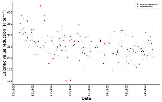
Figure 1.
Reference dataset of 170 sampled values of calorific value reduction (). Red diamonds: direct measurements (n = 21); blue dots: surrogate values (n = 170).
2.4. Mock Experiments
The use of a large and dense dataset is necessary for the training and validation of any ANN model. The experimental design must generate the data points needed to make a valid mapping of the predictor to response variables as assessed by a low value of the error function and the high accuracy of the predictions made using the model. An industrial implementation of the proposed problem-solving approach would require an experimental dataset that fulfills three conditions: (i) the dataset is acquired during operation over a wide range of relevant parameter values; (ii) the dataset is as large and as dense as possible; and (iii) the dataset can be acquired within the technical and economic constraints of the available resources. These requirements could be met using standard probes and data acquisition devices and by manipulating mechanical parameters in a bioreactor test unit designed for this purpose. However, the experimental data described above were acquired before deciding to use ANN models. Consequently, the mechanical set points were not varied, and the size of the experimental dataset is too small to be used to train ANN models. In order to overcome this limitation, additional data derived from mock experiments that use variation of the mechanical set points can be generated for the purpose of demonstrating the approach.
Hence, a mock dataset was created, comprising response values () derived from the experimental reference dataset obtained using the UAF test unit and four predictors: the actual influent flow rate Q and three mechanical factors that were previously described—i.e., the packing equivalent spherical diameter , the packing material type , and the fixed bed height/diameter ratio . The response values, of the mock dataset were obtained by multiplying the calorific value reduction of the reference dataset by a set of coefficients representing the possible effects of the three mechanical factors as shown in Equation (4).
where:
- = a vector of calorific value reductions for a single mock experiment;
- = the influent flow rate on the ith day;
- = the change in the calorific value of the influent stream on the ith day of the reference experiment;
- = the spherical diameter effects on calorific value reduction on the ith day;
- = the material type effects on calorific value reduction on the ith day;
- = the height-to-diameter effects on calorific value reduction on the ith day.
The effects due to a different spherical diameter, material type and height-to-diameter were derived from observations reported in the literature. A detailed description of the method used to generate the mock data and the references on which the ad hoc method are based are available in a separate document containing Supplementary Materials.
2.5. Experiment Plan to Obtain the Mock Experimental Dataset
The most efficient experimental plan should generate the dataset required to make an accurate ANN model in short duration with few experiments. Orthogonal arrays have the property that in every pair of columns, each of the possible ordered pairs of elements appears the same number of times [34]. The Taguchi arrays are a well-known set of orthogonal experiment designs that have demonstrated their usefulness in making predictive models. The Taguchi L9 experimental plan with four factors set to three different levels requires nine experiments [35]. With reference to the Taguchi L9 layout, a surrogate dataset for use in making an ANN model was generated using only three mechanical factors set to three levels. The fourth factor, the experimentally obtained influent flow rate, was a continuous vector without discrete levels. The influent flow rate comprises all the changes in the input material flux and is the only predictor that changes during an experiment Consequently, the influent factor levels change in an uncontrolled way. The same influent profile was used in each of the nine mock experiments.
Since each mock experiment had 170 sample points, the total number of response data points was 1530 (). The total number of predictors (4 factors) was 6120 (). Figure 2 shows the reference dataset of daily (black cross) and the response values from nine separate mock experiments. The density curves on the right side of Figure 2 show that the response values of the mock experiments were distributed over a wide range. The experimental plan with the levels of the mechanical factors and the corresponding response values (median and mean ± SD) for each mock experiment are presented in Table 1. This table also shows the rank of the mock experiments. The higher the value of , the better the treatment effectiveness.
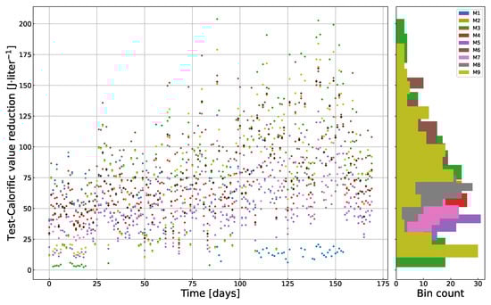
Figure 2.
Daily calorific value reduction (). Reference experiment and surrogate data for 1530 sample points from the mock experiment plan. On the righthand side, there are the binned calorific value reductions of the corresponding mock experiments. Black crosses show the reference data points.

Table 1.
Experimental plan (mock experiments). Three levels for each mechanical factor. The same influent profile was used in all the mock experiments. : equivalent spherical diameter (in mm); : packing material type (TWD: torrefied wood chips, PUF: polyurethane foam, PVC: polyvinyl chloride); : bed height/diameter ratio. The response data are median (mean ± SD) values (daily calorific value reduction) computed for each mock experiment distribution (see Figure 2).
2.6. Data Preprocessing
The data from the mock experiments were preprocessed to obtain a single dataset for use in training and validating all the models. The Scikit-learn [36], Matplotlib [37], Pandas [38], and Scipy [39] libraries were used for data processing and plotting.
The null hypothesis that the sample calorific value reductions are normally distributed was tested using the Shapiro–Wilk test. The calculated statistic of 0.965 indicates that the sample distribution is not normal (p-value < ). The calorific value reductions from the mock experiments are skewed to the right (sample statistic = 0.77). The kurtosis value (0.77, Fisher definition) indicates that the distribution of calorific value reductions has a longer tail than a normal distribution. To obtain a distribution closer to normal, the z-score, log, log(1+y), and the Yeo–Johnson transformations were compared. The Yeo-Johnson transformation of the response data from the nine mock experiments was found to yield the distribution that is the closest to normal (Shapiro–Wilk statistic = 0.997, p-value = 0.00198). The predictor data were not transformed.
Then, the complete predictor and response value datasets were Min–Max scaled to the range [0, 1]. The prediction accuracy of an MLP model with five hidden layers with 256 units per hidden layer was assessed in terms of RMSE and R.
Compared to training an MLP with raw mock data, training with transformed data improved the accuracy of the predictions. Consequently, the raw data pre-processing during further model development and simulation included the Yeo–Johnson transformation of the response data.
Then, the dataset was split into training and validation sets with a ratio of 80:20, and, respectively, 1224 and 306 sets of predictor and response values corresponding to 1530 sampling events (days). The Kolmogorov–Smirnov statistic (K-S) ks_2samp [39] on two samples was computed to test the null hypothesis that the training and validation response datasets were drawn from the same source. The null hypothesis can be rejected at the 99.9% confidence level if the K-S statistic is greater than the critical value (D) of 0.12. The calculated K-S statistic of 0.051 is less than the critical value (p-value = 0.53). Thus, the training and the validation response value datasets have the same distribution and were drawn from the same source.
Depending on the study objectives, the time-series order of the dataset was preserved or shuffled. The shuffle parameter was set to False when the temporal features of an experiment were preserved and to True when the temporal features of an experiment were not included in the dataset. Random_state was set to 42 to assure that the preshuffling operation was always the same.
2.7. Predictive Models
The selection of an appropriate predictive model depends on the intended use of the model and on the features of the dataset. In this study, the intended use was to predict a continuous response. Since this is a regression problem, a polynomial regression model was compared to a multilayer perceptron (MLP). Time-series datasets have features that vary over different time periods. In the context of this study, the type of variations include seasonal temperature changes and differences in the flow rates and composition between the day, the night and weekends. Different modeling strategies that include long short-term memory (LSTM) layers, for example, were developed to exploit the specific features of time-series datasets. In contrast, the multilayer perceptron (MLP) architecture is not specifically designed to account for temporal features. Consequently, the model selection approach included an analysis of time dependency, an assessment of conventional regression analysis with a polynomial model, and a comparison to the LSTM and MLP ANN architectures. The LSTM model proved to be less accurate than the MLP model when trained and tested using preshuffled data. Model training with an unshuffled time series dataset is not useful when the aim is to build a model for use in simulating different test cases. Since the aim of this work was to evaluate different predictor values by simulation, the LSTM strategy of response feature modeling was abandoned. The LSTM model and results are presented in the complementary information.
2.7.1. Polynomial Model
A fourth-order regression equation that mapped four predictors to calorific value reduction was fit to unshuffled time series data and then to data that were preshuffled. In both cases, 100 replicate runs were executed using the leave-one-out method to introduce randomness between runs.
The number of regression coefficients was arbitrarily chosen with reference to the four experimentally manipulated predictors. The variance inflation factors (VIFs) were calculated to test for the multicollinearity of the predictor variables. The VIF evaluates the variance of the estimated coefficients and increases to greater than 10 when the predictor variables are highly correlated and values greater than 4 should be investigated [40].
The evaluated array comprised four columns, each representing a predictor variable before Min–Max scaling, and 1530 rows representing the nine experiments (170 × 9 = 1530). The calculated variance inflation factors for ESD, MAT, HDR and influent flow were, respectively: 2.3, 2.0, 2.8, and 3.8.
2.7.2. Multilayer Perceptron (MLP) Model
The multilayer perceptron (MLP) ANN models were built using Python 3.7.6 and the Keras 2.3.0 API running on top of the TensorFlow 2.0 library for machine learning. The sequential model architecture was used. The input object shape was set to 4 (input_shape = (4,)). The input object received a single input array containing four vectors corresponding to the four predictors (ESD, MAT, HDR, Q). The output from the input object was passed to the first hidden layer comprised of dense units. The subsequent MLP hidden layers were constructed using identical dense units.
The accuracy of an ANN model can depend on the values of a unique set of weights determined by a single model training and validation run. Since the aim was to develop a general method to build ANN models for use in simulation, the focus was on the model architecture and not on the weights that were obtained from a particular training run. To do this, the initializer seed was set to None so that the unit weights were reinitialized before every model build, train, and test operation.
Different MLP models were built using an iterative process of adding layers and units, setting hyper-parameter values, and evaluating the prediction accuracy. The preliminary best result was a model having 6 hidden layers, each with 192 units per layer. Using this model, different hyper-parameters were then evaluated using semi-automated trials. The RMSprop optimizer [41] was found to perform slightly better than the Adam optimizer. The RMSprop training algorithm maintains a moving average of the square of gradients and divides the gradient by the root of this average. The learning rate was set as low as 1 , which is only 1% of the default value of 1 . The discounting factor for the history/incoming gradient, (rho) was set as high as 0.99 which is higher than the default value of 0.90. The momentum applied to the optimizer was set as high as 0.9.
The layer hyperparameters use_bias and bias_initializer were set to True and zeros, respectively. The TruncatedNormal initializer with a mean set to 0.0 and stddev set to 0.1 was used to set the initial weights of the hidden layers. The final hyperparameters settings were as follows: learning rate = , rho = 0.99, momentum = 0.05, epsilon = , centered = True. The learning rate was 10 times less and the momentum slightly more than the default values.
Regularization was applied using dropout. Drop-out layers were placed between the hidden layers to remove a fraction of the preceding layer’s units. The rate argument sets a fraction of the drop-out layer units to zero during training. Setting the different percentages [0.1, 1, 2, 3, 4, 5, 10, 25] of the dropout layer units to zero was evaluated. The final model had four dropout layers with the rate argument set to 0.05 (5% set to 0) in each layer.
The model output layer comprised a single dense unit connected to all the units of the preceding hidden layer, and with neither weights, nor bias, nor hyperparameters.
The compiled regression models were trained using a mini-batch gradient descent back-propagation learning algorithm. The default Keras MeanSquaredError class instance argument was used to output the average loss of each batch and was also used to evaluate the loss during each training epoch.
I only observed a small improvement in the prediction accuracy when more than 40 samples were used for model training.
Batch size of 1, 2, 4, 8, and 16 (days) were tested. Batch sizes of 1, 2, and 4 days resulted in the same accuracy. Setting the batch size to 8 or 16 days resulted in lower accuracy. I selected a batch size of four for the final model.
To determine the number of hidden layers and hidden layer units, all possible MLP architectures having between 1 and 13 hidden layers and between 8 and 4096 units per hidden layer were built, trained, and evaluated. Model building, training, and evaluation were repeated for each combination of layer and node numbers with the random initialization of the model weights. At the University of Lausanne high-performance computing center, 130 runs were then executed in 4 h using 1 NVIDIA A100 GPU and 10 GB of memory. The prediction accuracy of the validation tests was evaluated in terms of the coefficient of determination (R) and the slope of the regression line. There were small differences in the accuracy of the predictions between different model rebuilding operations. The models with more than 512 units per layer were frequently less accurate than the other models. The models with between 32 and 512 units per layer and between 2 and 6 hidden layers yielded similar and acceptable results.
2.8. Use of the Model for Simulation
The study hypothesis that the artificial neural network model can be used to distinguish different sets of up flow anaerobic filter constructive feature set point values by simulation was tested after building the model. The capacity to distinguish different constructive features was evaluated using a t-test. The results section contains a complete description of the method.
3. Results
Since all the models were evaluated using the same test data, the most appropriate model can be selected based on the accuracy of the predictions. The accuracy of the predictions was evaluated in terms of the root-mean-square error (RMSE) metric, which is calculated from the differences between true and predicted response values, the coefficient of determination (R2), and the slope of the regression line of predicted and true values. Both the polynomial and the MLP models were built, trained and validated separately using both the unshuffled time series and preshuffled data sets. The plots of predicted versus true values are shown in Figure 3 (unshuffled) and Figure 4 (preshuffled).
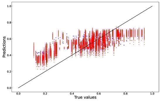
Figure 3.
True versus predicted values (unshuffled, true times series data); polynomial model: blue; MLP model: red.
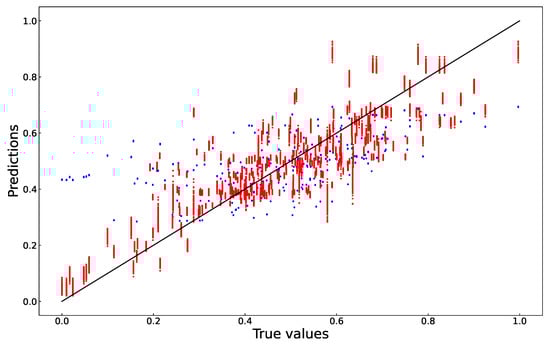
Figure 4.
True versus predicted values (preshuffled data); True versus predicted values (preshuffled data); Polynomial model: blue; MLP model: red.
To evaluate the prediction accuracy, 100 runs of the polynomial model were run using the leave-one-out method to introduce randomness between runs. The accuracy of the MLP model was assessed after making 100 training and validation runs with random weight initialization between runs. The results are shown in Table 2. The high slope and the small RMSE demonstrate the accuracy of MLP model. The small variation between runs demonstrates that the prediction accuracy is due to the architecture and not to a set of particular weights and thus contributes to the confidence of the results obtained by simulation.
Table 2.
Evaluation of model prediction accuracy.
3.1. Polynomial Model
In terms of RMSE and (R), the fourth degree polynomial model was less accurate than the MLP. When unshuffled, true time-series data were used to build the model, and the RMSE was 0.149. The coefficient of determination of a plot the validation test’s true and predicted values was 0.29. When preshuffled data were used to build the model, the RMSE was 0.140. The coefficient of determination of a plot the validation test’s true and predicted values was 0.37. As shown in Figure 3, the prediction accuracy was very low when the true values were less than 20% and more than 80% of the maximum.
3.2. MLP Model
When unshuffled data were used to build the model, the RMSE was 0.127. The coefficient of determination of a plot of the validation test’s true and predicted values was 0.48. When preshuffled data were used to build the model, the RMSE was 0.101. The coefficient of determination of a plot of the validation test’s true and predicted values was 0.66. Compared to the polynomial model, the range of accurately predicted values is greater in the MLP model. This difference is also shown in Figure 4 (preshuffled) by the higher slope of the MLP model compared to the polynomial model.
3.3. Time-Series Effects
To investigate the possible time series effects, the autocorrelation function was calculated for 100 days. The autocorrelation coefficient falls to and remains less than 0.5 after an initial 1-day lag and there is a small positive or negative autocorrelation of the time series data after day 16. The calculated Durbin–Watson test statistic (D) was 0.146. The maximum p-value of the correlation coefficient of each time lag, at the 95% level of confidence, was . Since the value of the test statistic (D) is less than 2, the time series of the daily calorific value reduction is positively autocorrelated. These two observations of the response data being autocorrelated imply that the data might have time-dependent features.
However, since the aim of this study was to build a model for use in simulation when fed previously unseen data, the effects of data shuffling and the results of the model validation tests must be considered. The effect of data shuffling prior to training using shuffled data was compared to the effect of training using the actual (not shuffled) time-series data. As shown in Figure 3 (unshuffled), Figure 4 (preshuffled), and in Table 2, the prediction accuracy of the polynomial and MLP models was higher when the models were trained using preshuffled data than when the models were trained using the unshuffled time-series data. The results of model validation tests are shown in Table 2. The predictions made by both the polynomial and the MLP models are less accurate when tested using true time-series data. These results indicate that the performance of the studied processes is not time-series-dependent, and that each day can be treated as an independent sampling point.
3.4. Model Selected for Use in Simulation
In terms of the RMSE, coefficient of determination (R), and slope of the regression line, the MLP model yielded a better result than the polynomial model when trained using preshuffled data.
To further compare the polynomial and the MLP models, a t-test was performed to test the null hypothesis that the populations of predictions made using the two different models are the same. The p-values were obtained from 100 runs of the polynomial and the MLP model with random weight initialization between runs. Assuming the equal variances of the two populations and using the Bonferroni correction for 306 samples, the analysis of the p-values showed that the populations are statistically different at the 0.01 alpha level.
The results of the evaluation of 100 replicates of the models in terms of validation mean RMSE, coefficient of determination (R), and slope of the regression line are shown in Table 2. Since the four-layer MLP trained using shuffled data was more accurate than the other type of models tested, it was selected for use in simulation.
Figure 5 shows the training and validation losses over 100 epochs. We observed that training and validation loss curves meet after 20 epochs. Although the training and test loss curves separate after 25 epochs, the test loss curve does not rise. The training loss curve decreases at a lower rate before flattening after 80 epochs. The observation that the validation loss does not increase while the training loss remains almost constant indicates that the model is not overfit.
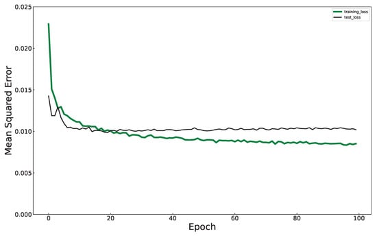
Figure 5.
Decrease of MAE during training and validation of the MLP model. Training loss: green; Test loss: black.
The outcome of model construction, evaluation, and tuning was the selection of the MLP architecture having 264,705 trainable parameters and 4 hidden layers, each with 512 identical dense units. The dataset was preshuffled. The four model input vectors were the packing spherical diameter, packing material type, packed bed height-to-diameter ratio, and the influent flow rate. The only model output was a vector of the daily calorific value reductions ( expressed in ) of the influent stream pollution load. After training the MLP model to achieve an acceptable loss during validation, the architecture and hyperparameters of the complied model were saved in HDF5 format for subsequent reloading and use for simulation.
3.5. Evaluation of the Experimental Plan
The experimental plan should generate predictions from independent experiments. If the predictors used in the mock experiments were not independent, then some of the experiments would be redundant and consequently bias the experimental results. Redundancy is manifested by the similarity of the response profiles. To investigate a possible redundancy in the experimental plan arrays, response datasets constructed using three different ways of combining two mock experiments were tested: (1) Taguchi-inspired experimental matrix; (2) removing one of the two most similar experiments; and (3) removing one experiment at random. The combination of nine experiments based on the L9 array described above was evaluated using the Kolmogorov–Smirnov test with a significance level set to 0.10 to assess the independence of all combinations of 2 mock experiments from the experimental plan. The corresponding value of the K-S test statistic was 0.18. Out of 36 possible combinations of 2 mock experiments, the calculated K-S statistic was greater than 0.18 in 3 cases. This implies that the experiments included in these three combinations might be redundant. The combination of experiments E3 and E9 had the highest p-value (0.44). Consequently, experiment E3 was removed from the experimental plan. To test the effect of removing the most redundant experiment, the MLP model was then built and evaluated with the experiment E3 removed.
To test the effect of removing a randomly selected experiment before each run, 100 replicates of the MLP model were run using a leave-one-out approach. The prediction accuracy was used to evaluate the effect of removing mock experiments from the experimental plan. Table 3 shows the tested combinations of mock experiments and the resulting RMSE and the coefficient of determination (R) of the predictions.
Table 3.
Experimental plans evaluated.
A slightly better result, in terms of RMSE and the coefficient of determination (R), was obtained when redundant experiment E3 was removed. The random removal of a single experiment increased the RMSE and reduced the coefficient of determination (R). The apparent redundancy in the experimental results might be due to real biological or physical causes expressed in the full L9 predictor dataset. For this reason, and because the Taguchi L9 array is a balanced array designed to consider all of the factors and levels equally and to specify a minimal number of experiments, no experiments were removed.
3.6. Use of the MLP for Simulation
The previously trained and saved MLP model was reloaded for use as a simulation tool to aid in designing UAF systems for specific use cases. The simulation tool can be used to select the best design specification from comparable simulated test cases. To do this, test cases were defined to explore the possible combinations of influent flow rate, packing material spherical diameter, type of packing material, and fixed bed height-to-diameter ratio within the range of the values used to train the model.
A full factorial design was used to specify a set of 125 permutations of the three mechanical parameters (factors) at five levels. In our simulation step, the high and low-level set-points used were the same as those used in the Taguchi L9 mock experiment design that was followed during the data generation step. The middle level value was the same as the value used during experimental data acquisition. The level values of the mechanical predictors are shown in Table 4.
Table 4.
Level values of the mechanical predictors.
For each simulation run, a new daily influent flow rate profile was created de novo using the NumPy random uniform generator. All values within the actual minimum and maximum values observed during data acquisition were equally likely to be drawn. To make a comparison between all possible experiments, the same daily influent flow rate profile was used in each experiment conducted during a single simulation run.
As shown in Figure 6, the number of binned influent flow rates observed during the period of data acquisition covered a wide range between 2 and 22 with modes around 200 and 460 L·day. Regarding the simulations, the number of binned influent flow rates varied within a more narrow range of between 3 and 14. The coefficient of variation within a bin ranged between 1.3% and 4.8%.
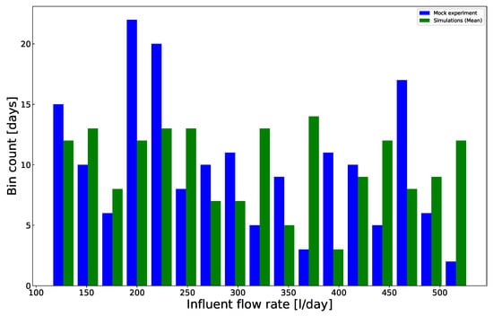
Figure 6.
Influent flow rate: experiments (blue bars); simulations (green bars).
A simulation run consisted in loading the previously built MLP neural network model and then feeding a (21,250, 4) tensor corresponding to 125 experiments of 170 days duration, each having four predictors. Bioreactor performance was evaluated in terms of the total calorific value reduction determined by the simulation. The number of replicate simulations required for a one-sided confidence interval (alpha/2) of 0.5% was estimated using the critical value from the normal distribution and the maximum sample standard deviation [42]. The minimum number of replicates is seven. The sum of the daily total predicted Min–Max scaled calorific value reduction was calculated for 20 replicates of the simulated experiments. The results of the 125 simulated experiments were then ranked according to the mean calorific value reduction.
The box plot (Figure 7) shows the means and the distribution of values within replications of a single experiment and the range of predicted cumulative total calorific value reductions. Identical influent streams were fed to all 125 experiments included in a single replication. However, each replication had a unique randomly generated influent stream flowrate profile.
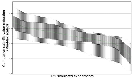
Figure 7.
Box plot of the predicted calorific value reduction. Results of 125 simulated experiments using the MLP model. The boxes enclose all values in the 25th through the 75th percentiles. The whisker reach is set to two times the range of boxes. The green lines show the mean of the simulation runs.
The null hypothesis of no difference between the means of the three highest ranking experiments was tested using a t-test and assuming equal variances in the sample populations. Simulated experiments SE125, SE119 and SE100 yielded the highest total calorific value reduction. Since the simulated experiment SE119 had the second highest ranking mean total calorific value reduction, the significance of the difference between SE125 and SE119 was tested. The calculated p-value of the difference between experiments SE125 and SE119 is 0.0108, indicating that the rejection of the null hypothesis is expected to be erroneous in much less than 2% of experiments. The calculated p-value of the difference between experiments SE125 and SE100 is 0.0027, indicating that the rejection of the null hypothesis is expected to be erroneous in less than 1% of experiments. Thus, the null hypothesis is rejected and the mechanical set point values used in experiment SE125 are expected to yield the highest total calorific value reduction during more than 98% of the tested influent flow regimes.
The spherical diameter was 36 in the 3 highest ranked experiments. In the three highest ranked experiments, the material type code was 1 or 1.85, indicating that the packing material with a smooth surface is appropriate. The height-to-diameter ratio was 4 in the 2 highest ranking experiments and 2.9 in the third highest ranking experiment. Consequently, the bioreactor should be long.
The same MLP model was reloaded and used to simulate influent flow rates in the low range of 127–321 L per day. The simulation results show that using the mechanical parameters ESD = 4, MAT = 11, and HDR = 4 results in the highest calorific reduction. Consequently, if the influent flow rate is low, then a small diameter and rough surfaced packing material should be used.
These design recommendations are based on mock data and are meant to only illustrate the method. The design recommendations are not meant for use in constructing a real upflow anaerobic filter. The design recommendation for use in constructing a real upflow anaerobic filter must be based on real measurements made during experiments.
4. Discussion
The method and workflow presented in this study are intended to improve the entire environmental bioprocesses development workflow from raw data collection to design specification. The present study demonstrates, for the first time, the workflow and use of an MLP as a simulation tool to specify constructive features of an upflow anaerobic filter. The contributions of this study are compared to existing work and the advantages of the proposed method are discussed below.
4.1. Comparison to Existing Methods
Many laboratory and industrial studies describe the use of numeric models for wastewater treatment system identification and process performance forecasting based on water quality parameters. For example, in the context of a study to optimize the operating cost of a large activated sludge wastewater treatment plant, Koncsos [43] built an MLP neural network model to predict the concentrations of components such as ammonium (NH-N) and nitrate (NO-N). The ANN model was trained and validated using a surrogate dataset generated using the variants of established activated sludge models (ASMs). For NH-N and NO-N, the correlation coefficients (R) of the predictions made by the ANN with ASM dataset were, respectively, 0.889 and 0.954. For suspended solids, expressed as COD, the correlation coefficients (R) of the ANN with ASM dataset were 0.987 for the 0–5 min interval and 0.843 for the 10–20 min future interval. In contrast, the intended use of the model built during the present study was simulation, and not operational process forecasting. Moreover, the purpose of simulation was to design equipment and not to optimize process control. The predictive model built during the present study did not include influent water quality parameters. The constructive features of the bioreactor and the influent flow rate were the only predictors of process performance. Additionally, the prediction interval was 170 days and the process performance was assessed by the cumulative calorific value reduction during this period rather than parameter prediction during a short interval. Forecasting models were also applied to anaerobic processes. For example, in a study of industrial starch processing wastewater treatment by an upflow anaerobic sludge blanket (UASB) bioreactor, Antwi et al. [44] built an MLP to predict COD removal from influent (COD, NH, pH, OLR) and effluent parameters (VFA and biogas yield) in the predictor dataset. The coefficient of determination (R) of the data reserved for testing was 0.87. This work is an accurate mapping of the selected prediction to response variables that helps to understand a complex process. In comparison, the present study did not include effluent parameters in the predictor dataset and the aim was to develop a simulation tool. With the goal of intensifying biogas production in a modern wastewater treatment plant, Sakiewicz et al. [45] built general regression neural network (GRNN), radial basis function (RBF) network and MLP models of data acquired during 3 years of continuous plant operation. This study focused on identifying the important parameters that affect process performance. Their analysis approach made it possible to conclude that the technical control process parameters have a more important influence on process performance than the wastewater quality indicators. Consequently, attention should be focused on mechanical features such as process control settings rather than on the wastewater stream quality and microbiological features of the anaerobic digestion process. Importantly, this result suggests that it might be possible to build a high-performance numerical model of technical environmental bioprocesses without the knowledge of the conventional water quality parameters and the biochemical parameters used in the IWA mathematical modeling approach. In contrast to the present study, they did not consider mechanical constructive features and they did not run simulations using neural network models.
Although less frequently used than operational parameters, some mechanical parameters have been included in numeric models of wastewater treatment processes. For example, the packing material dimension, packing material surface features, the bioreactor geometry and the influent flow rate are known to have an effect on UAF performance. Bolte et al. [46] included the flow rate, surface area and porosity of the support medium in a mathematical model used to simulate anaerobic filters treating dilute waste streams. In an expired patent [47], it is claimed that the diameter of the biomass support spheres must be sufficient to generate the surface shear forces required to shed microorganisms, and thereby prevent bed clogging. In a laboratory study of an upflow anaerobic packed bed reactor treating organic waste streams, Tay et al. [48] examined the significance of media factors such as media roughness, specific surface area, porosity and pore size on treatment performance. They found that media pore size and porosity play significant roles in the performance of the reactor. Different media types can have different pore sizes and porosity. For example, PVC has a smooth, non-porous surface, and foam can have a rough, porous surface. Consequently, different packing material diameters, material types, sizes and surface characteristics were investigated as predictors in the present study. Tests of anaerobic digestion of food industry wastewater in 10-liter anaerobic filters fed batches of influent from an industrial site showed that most of the organic substrates were used in the bottom of the reactor [49]. This implies that there is an optimal fixed bed length. If the fixed bed is too short, then the bioreactor is less effective. If the fixed bed is too long, then the bioreactor construction costs and the space requirements are unnecessarily high. These observations led to the decision to investigate the fixed bed height-to-diameter ratio during the present study. By integrating these important, and previously recognized, mechanical features into a single ANN predictive model, the present study contributes to the UAF design process.
Additionally, this study contributes to the development of methods to build and use neural networks in the field of environmental systems. In the present study, the intended use of the artificial neural network for simulation is very different from other possible uses such as fault detection or real-time forecasting. This use requires a predictive model that fits a large dataset acquired during a long time period. The suitability for use in the field of wastewater treatment, and in particular to model the upflow anaerobic filter, was an additional requirement. Considering these requirements, the polynomial, MLP, and LSTM models are among the natural candidates. Referring again to the study of Sakiewicz et al. [45], general regression neural network (GRNN), and the radial basis function (RBF) network and MLP models of data acquired during 3 years of continuous plant operation were built and evaluated. They determined that the MLP model with two hidden layers with 13 and 9 units per layer was the most accurate. In a laboratory study that compared the predictive ability of the numerical models of upflow anaerobic filters, Yilmaz [50] demonstrated that an MLP having only one hidden layer with six units more accurately predicted the methane yield than the conventional multi-linear regression or the Stover–Kincannon models. Using a surrogate dataset obtained from the simulations of an activated sludge wastewater treatment plant made using the ASM model, Demir [51] built an MLP neural network model to predict COD, phosphorus and nitrogen removal from the influent concentrations and operating parameters that control internal recycle. The coefficient of determination (R) of true to predicted values was between 0.95 and 0.99. This study showed how the design engineer can use the model to determine design and operational parameters by simulation and sensitivity analysis. Instead of using sensitivity analysis, we selected the design parameters by ranking the results of simulations made using all possible permutations of three design parameters. In the context of the forecast modeling of NO concentrations in wastewater treatment plants, Hwangbo et al. [52] observed that an LSTM model outperformed a DNN model in terms of forecast prediction accuracy. They noted that the LSTM-based forecasting modeling depends on the response data, whereas all sensor data can be used as predictors in DNN models. Consequently, they concluded that the LSTM-based model is not suitable for process modeling that includes every measured variable. This fundamental difference between the LSTM and MLP model architectures might explain the inaccuracy, in terms of (R), of the predictions made during the present study using the LSTM model. In agreement with this conclusion, the MLP model was selected for use in simulation during the present study. The accuracy and capacity of a numeric model for a specific use case, such as simulation, partly depends on the model architecture. Since there is no established methodology to determine the architecture, the subject is a popular research topic. Dibaba et al. [53] used a differential evolution (DE) approach to tune an ANN model of an upflow anaerobic contactor (UAC) for biogas production from vinasse. The ANN model predicted effluent chemical oxygen demand (COD), total suspended solids (TSSs), volatile fatty acids (VFAs) and biogas production from the characteristics of the influent vinasse. Their DE method involved the random manipulation of the MLP dimensions and hyperparameters and then selection of the best configuration based on the error. Using the DE method, the performance of the ANN model, in terms of the coefficient of determination (R), improved from 0.891 to 0.921. In comparison, the present study included a broad search and the evaluation of 130 different combinations of the number of hidden layers and units in order to select the optimal MLP architecture. A semi-automated trial and error approach to determine the best MLP hyperparameter settings in terms of the coefficient of determination (R). Building on this experience, MLP models having from 1 to 13 hidden layers and from 8 to 4096 units per layer. The time requirement to build and train a large neural network is no longer an issue. The selected neural network had 4 hidden layers, each having 256 units. This model was built and trained for 100 epochs in 3 h using a laptop (HP EliteBook 840 G4, Intel Core i5-7200U CPU@2.50 GHz, 8 Go RAM).
Forecasting a parameter value requires a model that maps predictor values, that change in time and often in an irregular way, to a response value. In contrast, a numeric model that simulates fixed mechanical values does not have to account for changes in the predictors. A model that simulates mechanical values is comparable to a physical prototype with features that closely resemble those of the final machinery. Prototype testing consists of executing an experimental plan to expose the physical device to the expected service conditions. Given the benefit of the close resemblance of the prototype to the final machinery, an overparameterized neural network might be desirable. The MLP used in this study was highly overparameterized with many more trainable model parameters than data points. Contrary to conventional practice, recent evidence has shown that there are significant benefits to having more parameters than data points when training a neural network [54]. The authors cite a state-of-the-art image recognition system, with a parameter-to-data point ratio of 400, as an example of such large-scale overparameterization. Early stopping during training results in an overparameterized neural network that is effective for interpolation. Consequently, the model used for simulation was highly overparameterized and trained until the number of epochs was sufficient to assure a low prediction error. The ratio of model parameters to data points was 35.
Although the present study did not aim to develop a soft sensor, the calorific value reduction could be considered as a composite parameter that describes process performance. ANN-based soft sensors are used to predict unmeasured or impossible to measure variables. For example, Pisa et al. [55] developed an MLP-based soft sensor to predict effluent total nitrogen since this parameter cannot be measured online. The prediction structure included LSTM cells that predicted effluent concentrations 4 h in the future based on input data from the previous 10 h. It is currently not possible to measure effluent calorific reduction online. The MLP predictive model developed during this study could be improved to build an ANN-based soft sensor for calorific value reduction.
4.2. Contribution of the Proposed Method
The conventional workflow to develop environmental bioprocesses could be improved, for example, by reducing the time and resource requirements for laboratory experimentation and by collecting data under real operating conditions. To meet this requirement, a data acquisition system was designed to make it possible to easily vary real mechanical features and to measure process parameters under real, industrial, operating conditions. This study demonstrated that it is not necessary to include conventional bioprocesses parameters such as kinetic constants, microbial inhibition factors, and hydrodynamic parameters that are difficult to measure in industrial conditions. For this reason, the proposed method can be described as a “black-box” approach.
Since the prediction accuracy of an ANN model depends on the number of raw data points, the data acquisition unit and the experimental plan should make it possible to acquire a very large dataset and to vary the relevant mechanical parameters. The most practical way to address this problem is to allow these parameters to naturally vary during the experiment thereby including the complexity of the industrial conditions in the dataset used to build the ANN. In the present study, the influent flow rate widely and irregularly varied during experimental data acquisition. The proposed method also takes advantage of advances in sensing and data acquisition techniques that make it possible to measure process parameters that might be meaningful when using the “black-box” approach but meaningless in a conventional dynamic chemical equilibrium approach to bioprocess modeling. Thus, the present study contributes to the movement towards the use of in-line measurement and data intensive methods during process development.
This study demonstrated that it is possible to acquire the data required to build a useful numeric model without laboratory experiments and that a balanced experimental array design can help to improve the prediction accuracy of the model. The experimental plan should reflect the highly variable quality of the influent wastewater stream in terms of composition, flow rate and temperature that, because of economic constraints, cannot be regulated in an industrial context. The use of a modified Taguchi experimental design to obtain a balanced array was demonstrated. However, any experimental design that leads to the development of a high-quality model can be used. The quality of any numerical model can be assessed by examining how closely model implementation agrees with the underlying physics of the studied subject, the prediction error as defined by the relative difference between the predicted value and the true measured value, and by the accuracy of the predictions made from data that represent a wide range of operating conditions. In the proposed approach, the underlying physics was accounted for by easily measured parameters such as exit gas and liquid flow rate and mechanical constructive features.
This study demonstrated the use of an ANN model of experimentally acquired data as a simulation tool to explore bioreactor performance under new conditions that were not experimentally tested. The present study demonstrates, for the first time, the workflow and use of a MLP to specify the mechanical constructive features of an upflow anaerobic filter. Using the proposed approach is expected to save time. The duration of the mock experimental phase was only 5.5 months, whereas the simulations covered more than 58 years of continuous operation.
The method and workflow demonstrated by this study are intended to be generally applicable to the design of the environmental process equipment and constructed natural systems.
4.3. Future Implementation
In future work, the proposed method could be implemented using three bioreactor test units operated simultaneously under real industrial conditions. The values of mechanical parameters would be set to cover the high and low extremes according to an experimental plan designed so that in every pair of columns, each of the possible ordered pairs of elements appears the same number of times as is characteristic of orthogonal arrays. The plan would also include the vectors of continuously varying process operational parameters such as flow rate or a water quality parameters that do not conform to the rules of orthogonal arrays. The experimental plan would be implemented to gather as many data points as possible during a short duration. For example, the influent flow rate and methane production measurements could be made continuously during 2 months. The resulting dataset would be used to build an MLP model for use in predicting the bioreactor performance under any set of simulation conditions lying within the range of values observed during the experiment. Thus, the model would make it possible to explore different equipment dimensions and operating set-point values that were not experimentally tested.
It is also possible to use the proposed method to model existing datasets. The methods of surrogate data generation described in this study and dataset reconfiguration could be used to create mock experiments.
5. Conclusions
This study demonstrated the development of a multilayer perceptron (MLP) artificial neural network (ANN) predictive model and its use to determine bioreactor mechanical design parameters by simulation. The main findings of this study were:
- The predictions made using the MLP were more accurate than those made using the polynomial model (coefficients of determination (R), respectively, of 0.66 and 0.37);
- The MLP model used for simulation should be defined by architecture and not by a particular set of hidden-layer unit weight initializations;
- The reloaded MLP model can be used for simulation using previously unseen input vectors;
- The differences in the predictions are significant (p-value < 0.02, range = mean ± 20% of the full range);
- The ranked order of simulation results can be used to select the set of mechanical specifications that will result in the highest equipment performance;
- A practical on-site data collection plan can be used to reduce the resource requirements for new process development.
The demonstration that different sets of mechanical design parameters yield significantly different predicted performance confirms the capacity of the model to distinguish differences in equipment design parameters. By making it possible to explore a wide range of mechanical parameter set points without costly and time-consuming laboratory experiments, the implementation of the method is expected to lead to improved, more efficient, design specifications of environmental bioprocessing equipment.
Supplementary Materials
The following are available online at https://www.mdpi.com/article/10.3390/su14137959/s1. References [49,56,57,58,59,60,61,62] are cited in the supplementary materials.
Funding
This study was funded by the Swiss Academy of Engineering Sciences (SATW), grant number 2020-001 https://www.satw.ch/en/ (accessed on 24 May 2022). M.M. was partially supported by Innosuisse—Swiss Innovation Agency and SCCER BIOSWEET https://www.innosuisse.ch/inno/en/home.html (accessed on 24 May 2022).
Institutional Review Board Statement
Not applicable.
Informed Consent Statement
Not applicable.
Data Availability Statement
The data presented in this study are available on request from the corresponding author.
Acknowledgments
Alessandro E.P. Villa contributed to the data analysis and neural network model methodology development.
Conflicts of Interest
The author declares no conflict of interest.
References
- IWA. International Water Association (IWA); IWA: London, UK, 2020. [Google Scholar]
- Dochain, D.; Vanrolleghem, P.A. Dynamical Modelling & Estimation in Wastewater Treatment Processes; IWA Publishing: London, UK, 2001; p. 9781780403045. [Google Scholar] [CrossRef]
- Barton, P.I.; Lee, C.K. Modeling, simulation, sensitivity analysis, and optimization of hybrid systems. ACM Trans. Model. Comput. Simul. 2002, 12, 256–289. [Google Scholar] [CrossRef]
- Dochain, D. (Ed.) Bioprocess Control; ISTE: London, UK, 2008; 248p. [Google Scholar]
- Ramaswamy, S.; Cutright, T.; Qammar, H. Control of a continuous bioreactor using model predictive control. Process Biochem. 2005, 40, 2763–2770. [Google Scholar] [CrossRef]
- Lima, F.V.; Rawlings, J.B. Nonlinear stochastic modeling to improve state estimation in process monitoring and control. AIChE J. 2011, 57, 996–1007. [Google Scholar] [CrossRef]
- Liotta, F.; Chatellier, P.; Esposito, G.; Fabbricino, M.; Van hullebusch, E.D.; Lens, P.N.L.; Pirozzi, F. Current Views on Hydrodynamic Models of Nonideal Flow Anaerobic Reactors. Crit. Rev. Environ. Sci. Technol. 2015, 45, 2175–2207. [Google Scholar] [CrossRef] [Green Version]
- Teixeira, A.P.; Alves, C.; Alves, P.M.; Carrondo, M.J.T.; Oliveira, R. Hybrid elementary flux analysis/nonparametric modeling: Application for bioprocess control. BMC Bioinform. 2007, 8, 30. [Google Scholar] [CrossRef] [Green Version]
- Zhang, Q.; Hu, J.; Lee, D.J.; Chang, Y.; Lee, Y.J. Sludge treatment: Current research trends. Bioresour. Technol. 2017, 243, 1159–1172. [Google Scholar] [CrossRef]
- Haimi, H.; Mulas, M.; Corona, F.; Vahala, R. Data-derived soft-sensors for biological wastewater treatment plants: An overview. Environ. Model. Softw. 2013, 47, 88–107. [Google Scholar] [CrossRef]
- Fisher, O.J.; Watson, N.J.; Porcu, L.; Bacon, D.; Rigley, M.; Gomes, R.L. Multiple target data-driven models to enable sustainable process manufacturing: An industrial bioprocess case study. J. Clean. Prod. 2021, 296, 126242. [Google Scholar] [CrossRef]
- Tetko, I.; Villa, A. An Enhancement of Generalization Ability in Cascade Correlation Algorithm by Avoidance of Overfitting/Overtraining Problem. Neural Process Lett. 1997, 6, 43–50. [Google Scholar] [CrossRef]
- Tetko, I.V.; Aksenova, T.I.; Volkovich, V.V.; Kasheva, T.N.; Filipov, D.V.; Welsh, W.J.; Livingstone, D.J.; Villa, A.E. Polynomial neural network for linear and non-linear model selection in quantitative-structure activity relationship studies on the internet. SAR QSAR Environ. Res. 2000, 11, 263–280. [Google Scholar] [CrossRef]
- Tetko, I.V.; Tanchuk, V.Y.; Kasheva, T.N.; Villa, A.E.P. Estimation of aqueous solubility of chemical compounds using E-state indices. J. Chem. Inf. Comput. Sci. 2001, 41, 1488–1493. [Google Scholar] [CrossRef] [PubMed]
- Harada, L.H.P.; da Costa, A.C.; Maciel Filho, R. Hybrid neural modeling of bioprocesses using functional link networks. Appl. Biochem. Biotechnol. 2002, 98–100, 1009–1023. [Google Scholar] [CrossRef]
- Ławryńczuk, M. Modelling and nonlinear predictive control of a yeast fermentation biochemical reactor using neural networks. Chem. Eng. J. 2008, 145, 290–307. [Google Scholar] [CrossRef]
- Rene, E.R.; López, M.E.; Kim, J.H.; Park, H.S. Back propagation neural network model for predicting the performance of immobilized cell biofilters handling gas-phase hydrogen sulphide and ammonia. BioMed Res. Int. 2013, 2013, 463401. [Google Scholar] [CrossRef]
- Sharghi, E.; Nourani, V.; Ashrafi, A.; Gökçekuş, H. Monitoring effluent quality of wastewater treatment plant by clustering based artificial neural network method. Pol. J. Environ. Stud. 2019, 164, 86–97. [Google Scholar] [CrossRef]
- Delnavaz, M.; Farahbakhsh, J.; Talaiekhozani, A.; Mehdinezhad Nouri, K. Predicting Removal Efficiency of Formaldehyde from Synthetic Contaminated Air in Biotrickling Filter Using Artificial Neural Network Modeling. J. Environ. Eng. 2019, 145, 04019056. [Google Scholar] [CrossRef]
- de Menezes, P.L.; de Azevedo, C.A.V.; Eyng, E.; Neto, J.D.; de Lima, V.L.A. Artificial neural network model for simulationof water distribution in sprinkle irrigation. Rev. Bras. Eng. Agrícola E Ambient. 2015, 19, 817–822. [Google Scholar] [CrossRef] [Green Version]
- Venkatesh Prabhu, M.; Karthikeyan, R. Comparative studies on modelling and optimization of hydrodynamic parameters on inverse fluidized bed reactor using ANN-GA and RSM. Alex. Eng. J. 2018, 57, 3019–3032. [Google Scholar] [CrossRef]
- Salehi, E.; Askari, M.; Aliee, M.H.; Goodarzi, M.; Mohammadi, M. Data-based modeling and optimization of a hybrid column-adsorption/depth-filtration process using a combined intelligent approach. J. Clean. Prod. 2019, 236, 117664. [Google Scholar] [CrossRef]
- Arismendy, L.; Cárdenas, C.; Gómez, D.; Maturana, A.; Mejía, R.; Quintero, M.C.G. Intelligent System for the Predictive Analysis of an Industrial Wastewater Treatment Process. Sustainability 2020, 12, 6348. [Google Scholar] [CrossRef]
- Witherow, J.L.; Coulter, J.B.; Ettinger, M.B. Anaerobic Contact Process for Treatment of Suburban Sewage. J. Sanit. Eng. Div. 1958, 88, 1–13. [Google Scholar] [CrossRef]
- Richard, R.; Dague, R.E.M.; Pfeffer, J.T. Anaerobic Activated Sludge. J. Water Pollut. Control Fed. 1966, 38, 220–226. [Google Scholar]
- Young, J.C.; McCarty, P.L. The anaerobic filter for waste treatment. J. Water Pollut. Control Fed. 1969, 41, 160. [Google Scholar]
- Genung, R.K.; Million, D.L.; Hancher, C.W.; Pitt, W.W., Jr. Pilot Plant Demonstration of an Anaerobic Fixed-Film Bioreactor for Wastewater Treatment; Oak Ridge National Lab.: Oak Ridge, TN, USA, 1978.
- Manariotis, I.D.; Grigoropoulos, S.G. Municipal-Wastewater Treatment Using Upflow-Anaerobic Filters. Water Environ. Res. 2006, 78, 233–242. [Google Scholar] [CrossRef]
- Córdoba, P.R.; Riera, F.S.; Sineriz, F. Temperature effects on upflow anaerobic filter performance. Environ. Technol. Lett. 1988, 9, 769–774. [Google Scholar] [CrossRef]
- Young, J.C. Factors Affecting the Design and Performance of Upflow Anaerobic Filters. Water Sci. Technol. 1991, 24, 133–155. [Google Scholar] [CrossRef]
- Bhattacharya, J.; Dev, S.; Das, B. Design of Wastewater Bioremediation Plant and Systems. In Low Cost Wastewater Bioremediation Technology; Butterworth-Heinemann: Oxford, UK, 2018; pp. 265–313. [Google Scholar]
- Zhu, G.Y.; Zamamiri, A.; Henson, M.A.; Hjortsø, M.A. Model predictive control of continuous yeast bioreactors using cell population balance models. Chem. Eng. Sci. 2000, 55, 6155–6167. [Google Scholar] [CrossRef]
- Tarjányi-Szikora, S.; Oláh, J.; Makó, M.; Palkó, G.; Barkács, K.; Záray, G. Comparison of different granular solids as biofilm carriers. Microchem. J. 2013, 107, 101–107. [Google Scholar] [CrossRef]
- Kacker, R.N.; Lagergren, E.S.; Filliben, J.J. Taguchi’s Orthogonal Arrays Are Classical Designs of Experiments. J. Res. Natl. Inst. Stand. Technol. 1991, 96, 577–591. [Google Scholar] [CrossRef]
- Roy, R.K. A Primer on the Taguchi Method, 2nd ed.; Society of Manufacturing Engineers: Dearborn, MI, USA, 2010. [Google Scholar]
- Pedregosa, F.; Varoquaux, G.; Gramfort, A.; Michel, V.; Thirion, B.; Grisel, O.; Blondel, M.; Prettenhofer, P.; Weiss, R.; Dubourg, V.; et al. Scikit-learn: Machine learning in Python. J. Mach. Learn. Res. 2011, 12, 2825–2830. [Google Scholar]
- Hunter, J.D. Matplotlib: A 2D Graphics Environment. Comput. Sci. Eng. 2007, 9, 90–95. [Google Scholar] [CrossRef]
- McKinney, W. Data Structures for Statistical Computing in Python. In Proceedings of the Python in Science Conference, Austin, TX, USA, 28 June–3 July 2010; van der Walt, S., Millman, J., Eds.; SciPy: Austin, TX, USA, 2010; pp. 56–61. [Google Scholar] [CrossRef] [Green Version]
- Virtanen, P.; Gommers, R.; Oliphant, T.E.; Haberland, M.; Reddy, T.; Cournapeau, D.; Burovski, E.; Peterson, P.; Weckesser, W.; Bright, J.; et al. SciPy 1.0: Fundamental Algorithms for Scientific Computing in Python. Nat. Methods 2020, 17, 261–272. [Google Scholar] [CrossRef] [Green Version]
- Iain Pardoe, L.S.; Young, D. STAT 462 Applied Regression Analysis. 2021. Available online: https://online.stat.psu.edu/stat462/node/180/ (accessed on 24 May 2022).
- Hinton, G.; Srivastava, N.; Swersky, K. Neural Networks for Machine Learning Lecture 6a Overview of mini- --Batch gradient descent. Cited 2012, 14, 2. [Google Scholar]
- NIST. NIST/SEMATECH e-Handbook of Statistical Methods, Section 7.2.2.2. 2021. Available online: https://www.itl.nist.gov/div898/handbook/prc/section2/prc222.htm (accessed on 14 March 2022).
- Koncsos, T. Bioreactor Simulation with Quadratic Neural Network Model Approximations and Cost Optimization with Markov Decision Process. Period. Polytech. Civ. Eng. 2020, 64, 614–622. [Google Scholar] [CrossRef]
- Antwi, P.; Li, J.; Meng, J.; Deng, K.; Quashie, F.K.; Li, J.; Boadi, P.O. Feedforward neural network model estimating pollutant removal process within mesophilic upflow anaerobic sludge blanket bioreactor treating industrial starch processing wastewater. Bioresour. Technol. 2018, 257, 102–112. [Google Scholar] [CrossRef] [Green Version]
- Sakiewicz, P.; Piotrowski, K.; Ober, J.; Karwot, J. Innovative artificial neural network approach for integrated biogas—Wastewater treatment system modelling: Effect of plant operating parameters on process intensification. Renew. Sustain. Energy Rev. 2020, 124, 109784. [Google Scholar] [CrossRef]
- Bolte, J.P.; Nordstedt, R.A.; Thomas, M.V. Mathematical Simulation of Upflow Anaerobic Fixed Bed Reactors. Trans. ASAE 1984, 27, 1483–1490. [Google Scholar] [CrossRef]
- Trösch, W.; Kiefer, W.; Lohmann, K.; Dürolf, H. Porous Inorganic Support Spheres Which Can Be Cleaned of Surface Biomass under Fluidized Bed Conditions. U.S. Patent 4,987,068, 22 January 1991. [Google Scholar]
- Joo-Hwa, T.; Kuan-Yeow, S.; Jeyaseelan, S. Media Factors Affecting the Performance of Upflow Anaerobic Packed-Bed Reactors. Environ. Monit. Assess. 1997, 44, 249–261. [Google Scholar] [CrossRef]
- Berardino, S.D.; Costa, S.; Converti, A. Semi-continuous anaerobic digestion of a food industry wastewater in an anaerobic filter. Bioresour. Technol. 2000, 71, 261–266. [Google Scholar] [CrossRef]
- Yilmaz, T. Modeling the performance of upflow anaerobic filter (UAF) reactors treating paper-mill wastewater using neural networks. Sci. Res. Essays 2013, 8, 1896–1905. [Google Scholar]
- Demir, S. Artificial Neural Network Simulation of Advanced Biological Wastewater Treatment Plant Performance. Sigma J. Eng. Nat. Sci. 2020, 38, 1713–1728. [Google Scholar]
- Hwangbo, S.; Al, R.; Chen, X.; Sin, G. Integrated Model for Understanding N2O Emissions from Wastewater Treatment Plants: A Deep Learning Approach. Environ. Sci. Technol. 2021, 55, 2143–2151. [Google Scholar] [CrossRef]
- Dibaba, O.R.; Lahiri, S.K.; T’Jonck, S.; Dutta, A. Experimental and Artificial Neural Network Modeling of a Upflow Anaerobic Contactor (UAC) for Biogas Production from Vinasse. Int. J. Chem. React. Eng. 2016, 14, 1241–1254. [Google Scholar] [CrossRef]
- Thomson, N.C.; Greenwald, K.; Lee, K.; Manso, G.F. The Computational Limits of Deep Learning. arXiv 2020, arXiv:2007.05558. [Google Scholar]
- Pisa, I.; Santín, I.; Vicario, J.; Morell, A.; Vilanova, R. ANN-Based Soft Sensor to Predict Effluent Violations in Wastewater Treatment Plants. Sensors 2019, 19, 1280. [Google Scholar] [CrossRef] [Green Version]
- Araujo, P.; Astray, G.; Ferrerio-Lage, J.A.; Mejuto, J.C.; Rodriguez-Suarez, J.A.; Soto, B. Multilayer perceptron neural network for flow prediction. J. Environ. Monit. 2011, 13, 35–41. [Google Scholar] [CrossRef]
- Hochreiter, S.; Schmidhuber, J. Long Short-Term Memory. Neural Comput. 1997, 9, 1735–1780. [Google Scholar] [CrossRef]
- Smith, L.C.; Elliot, D.J.; James, A. Mixing in upflow anaerobic filters and its influence on performance and scale-up. Water Res. 1996, 30, 3061–3073. [Google Scholar] [CrossRef]
- Olah, C. Understanding LSTMs. 2015. Available online: https://colah.github.io/posts/2015-08-Understanding-LSTMs/ (accessed on 14 March 2022).
- Escudié, R.; Conte, T.; Steyer, J.P.; Delgenès, J.P. Hydrodynamic and biokinetic models of an anaerobicfixed-bed reactor. Process Biochem. 2005, 40, 2311–2323. [Google Scholar] [CrossRef]
- Seabold, S.; Perktold, J. Statsmodels: Econometric and statistical modeling with python. In Proceedings of the 9th Python in Science Conference, Austin, TX, USA, 28 June–3 July 2010. [Google Scholar]
- Thirumurti, D. Effects of mixing velocity on anaerobic fixed film reactors. Water Res. 1988, 22, 517–523. [Google Scholar] [CrossRef]
Publisher’s Note: MDPI stays neutral with regard to jurisdictional claims in published maps and institutional affiliations. |
© 2022 by the author. Licensee MDPI, Basel, Switzerland. This article is an open access article distributed under the terms and conditions of the Creative Commons Attribution (CC BY) license (https://creativecommons.org/licenses/by/4.0/).