Spillover Effect of the Interaction between Fintech and the Real Economy Based on Tail Risk Dependent Structure Analysis

Abstract

Fintech innovation has greatly improved the operation efficiency of the financial industry and promoted the sustainable development of the real economy. On the other hand, fintech also brings the problem of risk spillover. Through a time series analysis, vector auto-regression with the Granger causality test is conducted to analyze the interaction between fintech and the real economy. To deal with the nonlinear relationship and overcome the high-dimensional-dependent structure faced by Copula, this paper establishes a GARCH–Vine–Copula model to study the tail risk and dynamic dependency between fintech and industries of the real economy in China, and then analyzes the risk spillover by calculating the CoVaR. The results show that there is a positive dynamic correlation between fintech and the real economy, and this increases when facing risk impact; fintech is located in the leading position of R-vine-dependent structure, and has a high correlation coefficient with the upper and lower tail of various industries. The results of CoVaR show that the extreme risk events in fintech and various industries have different degrees of negative impact on each other; the risk events in fintech have an extreme impact on industry in a short time.

1. Introduction

In terms of financial technology (fintech), the concept of fintech has not formed a unified definition. The accepted definition is that financial innovation is mainly driven by new cutting-edge technologies, such as big data, blockchain, cloud computing and artificial intelligence, and has a significant impact on the financial market and the supply of financial services.

Under the trend and background of economic globalization and financial market integration, the economic ties between different countries, regions and industries have become closer, and the financial information, financial resources and financial markets have been continuously integrated [1]. Industry 4.0, the fourth industrial revolution, has attracted much attention in the past decades. It is closely related to the Internet of Things (IoT), information and communications technology (ICT), Cyber Physical System (CPS), Enterprise Architecture (EA), Enterprise Integration (EI), and so on. At the same time, financial technology has also developed rapidly with industry 4.0 [2].

In recent years, with the growing maturity and wide application of cloud computing, artificial intelligence, blockchain, big data and other technologies, financial technology has become the core driving force to promote modern financial innovation. The traditional financial mode has undergone disruptive changes, and the financial industry has begun to show some new risk characteristics. Specifically, the innovation of financial products, the change of financing mode and the change of financial business model brought by fintech have greatly promoted the operational efficiency of the financial industry. Excessive innovation in the financial market has led to a significant increase in the complexity of financial products and financial transactions. Various financial institutions, including non-financial institutions, have become increasingly close to each other in terms of equity and debt, business cooperation and penetration, forming a complex financial network structure, and the contagion characteristics of the systematic financial risk network have become more and more obvious [3].

Real economic risks are also transmitted to the financial system. In the age of optimization and upgrading of industrial structure and economic transformation, the demand for traditional products is sluggish, and the market demand for technological innovation products is in the cultivation period. The common pressure of domestic and foreign markets has significantly reduced the profitability of enterprises. In order to maintain business operations, the high loan interest has increased the financial burden of the real economy, and the long-term “borrowing the new to repay the old” has intensified the risks of fintech [4].

2. Literature Review

In the study of the impact of fintech development on economy growth, the multivariate regression approach is commonly used. For example, Chen et al. [5,6] investigated how fintech affects the digital economy and if the digital economy can promote fintech development. Shin and Choi [7] studied the feasibility of the fintech industry as an innovation platform for sustainable economic growth in Korea. Tian, Li and Yang [8] made an empirical analysis of the impact of fintech on the development of the real economy and found that there is an interaction between them. Sun and Zhang [9] explained the internal mechanism of fintech innovation affecting economic growth and found that financial innovation in promoting economic growth through technological progress is significant. Thorsten, Tao and Chen [10] assessed the relationship between fintech and the development of a real economy, and found that the net effect is positive. Lee and Yong [11] evaluated fintech innovation and argued that its effect will cause output changes to the whole financial and economic ecosystem, which will lead to new challenges in investment decision making.

In the study of risk caused by fintech development, scholars such as Rafal and Daniel [12] revealed that the development of fintech not only improves financial efficiency, but also changes the existing form and transmission path of the original financial risk, which makes the transmission of traditional financial risk more hidden, complex and infectious under the load of emerging technologies, and breeds new financial risks. When extreme risk events occur in fintech, industries in real economies may be affected by their risk spillover, threatening the healthy development of the real economy. Vucinic and Luburic [13] examined the latest developments in the area of fintech and outlined the potential benefits and associated risks, and highlighted the cyber risk in the fintech landscape as the latest and potentially greatest threat springing from these turbulent and uncertain times. Chen et al. [14] investigated the spillovers between internet finance and traditional finance, and found that the linkage relationships and spillover effect are robust to the method and market index applied. Namchoochai et al. [15] adopted the principles of sustainable risk management for both providers and users who demand to use fintech with high security. The results indicate that the risks are relevant, and the difference in the level of risk depends on the details of each fintech type and the part of the business with which technologies are associated.

In the modeling of risk spillover, the most popular method is Copula–CoVaR. For example, Saraji et al. [16] developed a Fermatean fuzzy critic–copula method to identify the challenges for the adoption of Industry 4.0 in fintech companies, and to evaluate the performance of companies concerning the weighted challenges based on three decision experts’ support. The results indicate that “difficulty in coordination and collaboration” is the most significant challenge to the adoption of Industry 4.0. Yu and Wang [17] constructed the quality index system of economic growth in the new era by using the TOPSIS–copula method. The research found that when the matching degree between fintech and the real economy is low, it destroys financial stability. On the contrary, fintech achieves high quality economic growth by improving enterprise innovation ability and industry technical efficiency. Lin and Zhao [18] discussed the risk spillover effect between markets based on the time-varying Copula–CoVaR model, and the results showed that the risk effect is a two-way interaction. Karimalis and Nokimos [19] used the Copula–CoVaR approach to measure the systemic risk of European banks and believed that there was a significant risk spillover problem in financial innovation.

Since multivariate copula has parameter constraints and lacks the flexibility of dependency in modeling, scholars such as Joe, Sriboonchitta, Alanazi, Bedford, Zhu, Schepsmeier et al. [20,21,22,23,24,25] tried to improve the standard copula by integrating the vine approach. In the application of the vine–copula, Kim et al. [26] used the mixture of D-vine copulas for modeling dependence. Nikoloulopoulos and Karakas et al. [27,28] used the vine–copula form to model asymmetric tail dependence in stock markets. Autchariyapanitkul et al. [29] used C-vine and D-vine copulas to exhibit portfolio risk structure in the content of asset allocation. Czado, Schepsmeier and Min [30] created a flexible class of mixed C-vine copula models which allows the variables to be ordered according to their influence. Zhang [31] studied the price correlation structure of domestic urban real estate from a macro perspective based on the C-Vine Copula model. Reboredo and Ugolini [32] used a vine copula model and found that the dependence structure differed across precious metals, all of which displayed different average and tail dependence features. Guo [33] described the linkage relationship of China’s stock market with the vine copula GJR SKT model and concludes that the goodness-of-fit with the D-vine copula model is better. Zhang, Yan and Tsopanakis [34] utilized an R-vine copula method to explore tail dependence between the Financial Stress Indices of 11 countries in the euro area.

From the previous literature review, we mainly focus on fintech development and its driving effect on economy growth, the risk transmission mechanism and the quantitative analysis method. In the study of fintech’s promotion of the economy, many scholars have adopted exploratory factor analysis, confirmatory factor analysis, DEA and so on. Obviously, these methods are not suitable for risk analysis. Instead, the time series approach and CoVaR method are commonly used. When the relationship between variables is nonlinear, it is not reliable to measure the relationship with a correlation coefficient. Therefore, the copula approach can be used to model the tail risk for time series, however, the Copula also faces great challenges in dealing with high-dimensional problems because the standard multivariate copula’s structure is inflexible. A vine–copula can overcome such a limitation and is able to decompose the complex dependency patterns into multiple bivariate copulas.

Based on the existing research results, this paper intends to make the following marginal contributions. Firstly, we focus the research perspective on the dependent structural relationship between fintech and the real economy based on the industries’ stock index. The fintech index and the real economy index are constructed by imitating the s&p500 and CSI300 index; they are used to represent the fintech and the real economy in this study, respectively. Secondly, through a time series analysis, vector auto-regression with a Granger causality test is conducted to analyze the interaction between fintech and the real economy. Thirdly, to make up the deficiency of the copula model, which was applied to two-dimensional scenarios, we develop a GARCH–Vine–Copula–CoVaR model to make it more suitable for this study, and a case study is conducted. Fourthly, we select the R-vine copula model with strong flexibility to fit each standardized residual sequence after probability integral transformation, and estimate the parameters after obtaining the optimal pair–copula function through the AIC information criterion. According to the estimation results and the Kendall τ of the copula function, the values are sorted and the dependent tree of R-vine analyzes the relationship and tail dependence of various variables in detail. Finally, CoVaR, ∆CoVaR and %∆CoVaR are calculated to study the two-way risk spillover relationship between fintech and industries in the real economy.

3. Methodology

3.1. SVAR and Granger Causality Test

In order to judge the promotion between fintech (X) and the real economy (Y), this paper introduces the Granger causality test for analysis. Its principle is structural vector auto-regression (SVAR) for time series:

$$\begin{array}{c}{\mathrm{y}}_{\mathrm{t}}={{\displaystyle \sum }}_{\mathrm{i}=1}^{\mathrm{q}}{\mathrm{a}}_{\mathrm{i}}{\mathrm{x}}_{\mathrm{t}-\mathrm{i}}+{{\displaystyle \sum }}_{\mathrm{j}=1}^{\mathrm{q}}{\mathrm{b}}_{\mathrm{j}}{\mathrm{y}}_{\mathrm{t}-\mathrm{j}}+{\mathrm{u}}_{1\mathrm{t}}\\ {\mathrm{x}}_{\mathrm{t}}={{\displaystyle \sum }}_{\mathrm{i}=1}^{\mathrm{s}}{\mathsf{\Phi }}_{\mathrm{i}}{\mathrm{x}}_{\mathrm{t}-\mathrm{i}}+{{\displaystyle \sum }}_{\mathrm{j}=1}^{\mathrm{s}}{\mathsf{\omega }}_{\mathrm{j}}{\mathrm{y}}_{\mathrm{t}-\mathrm{j}}+{\mathrm{u}}_{2\mathrm{t}}\end{array}$$

(1)

where u_1t and u_2t are white noise; q and s both are the lagging periods.

If the past information of X and Y is included, the prediction effect of variable Y is better than that of Y alone, that is, variable X is helpful to explain the change of variable Y. Therefore, variable X is considered to be the Granger cause of variable Y. The test results are divided into the following four cases: (1) There is a one-way causal relationship from Y to X; (2) There is a one-way causal relationship from X to Y; (3) X and Y are cause and effect; (4) There is no causal relationship between X and Y

The Granger causality test is usually conducted by the constrained F test. If the calculated F value is greater than the critical value F_α(q, n − k) under the given significance level α of F distribution, then reject the original hypothesis, where n is the sample size and k is the number of variables to be evaluated.

3.2. GARCH Model

To better fit the residual tail characteristics of time series, the GARCH model is applied in this study as discussed by Heston and Nandi [35] and Ji, Wang and Liseo [36]. The modeling process of the GARCH model is divided into two parts: conditional mean regression and conditional heteroscedasticity regression. The equation form of GARCH (p, q) is as follows.

$$\begin{array}{c}{\mathrm{y}}_{\mathrm{t}}=\mathrm{c}+{\mathsf{\rho }}_1{\mathrm{y}}_{\mathrm{t}-1}+{\mathsf{\rho }}_2{\mathrm{y}}_{\mathrm{t}-2}+\cdots +{\mathsf{\rho }}_{\mathrm{n}}{\mathrm{y}}_{\mathrm{t}-\mathrm{n}}+{\mathsf{\mu }}_{\mathrm{t}}\\ {\mathsf{\mu }}_{\mathrm{t}}~\mathrm{N}\left(0,{\mathsf{\delta }}_{\mathrm{t}}^2\right)\end{array}$$

(2)

The variance equation is

$${\mathsf{\delta }}_{\mathrm{t}}^2={\mathsf{\alpha }}_0+{{\displaystyle \sum }}_{\mathrm{i}=1}^{\mathrm{p}}{\mathsf{\alpha }}_{\mathrm{i}}{\mathsf{\mu }}_{\mathrm{t}-\mathrm{i}}^2+{{\displaystyle \sum }}_{\mathrm{j}=1}^{\mathrm{q}}{\mathsf{\beta }}_{\mathrm{j}}{\mathsf{\delta }}_{\mathrm{t}-\mathrm{j}}^2$$

(3)

where p is the lag order in the arch term and q is the lag order in the GARCH; β is proposed to reflect the persistent impact of the variance change in the lag period on the current variance; μ_t is the error term.

3.3. Conditional Copula Function

Patton [37] proposed the conditional Copula model, which is specifically defined as [33]: W is the conditional variable of variables X and Y, and ${\mathrm{F}}_{\mathrm{XY}|\mathrm{W}}$ is the joint distribution function of conditional variable W; ${\mathrm{F}}_{\mathrm{X}|\mathrm{W}}$ is the conditional distribution function of variable X when W is known; Hypothesis ${\mathrm{F}}_{\mathrm{XY}|\mathrm{W}}$ is smooth and ${\mathrm{F}}_{\mathrm{X}|\mathrm{W}}$ and ${\mathrm{F}}_{\mathrm{Y}|\mathrm{W}}$are a continuous function; ${\mathrm{f}}_{\mathrm{W}}$ is the unconditional probability density function of W, then

$${\mathrm{F}}_{\mathrm{X}|\mathrm{W}}\left(\mathrm{x}|\mathrm{w}\right)={\mathrm{F}}_{\mathrm{XY}|\mathrm{W}}\left(\mathrm{x},\infty |\mathrm{w}\right),{\mathrm{F}}_{\mathrm{Y}|\mathrm{W}}\left(\mathrm{y}|\mathrm{w}\right)={\mathrm{F}}_{\mathrm{XY}|\mathrm{W}}\left(\infty ,\mathrm{y}|\mathrm{w}\right)$$

(4)

If $\mathrm{C}\left(·,·|·\right)$ satisfies the following conditions, it is a two-dimensional conditional Copula function:

Condition 1. 

C(u, 0|w) = C(0, v|w) = 0, C(u, 1|w) = u, C(1, v|w) = v; where u, v ϵ I.

Condition 2. 

u₁, u₂, v₁, v₂ are arbitrary variables of type I respectively, u₁ ≤ u₂, v₁ ≥ v₂, and C(u₂, v₂|w) – C(u₂, v₁|w) − C(u₁, v₂|w) + C(u₁, v₁|w) ≥ 0.

According to the Copula theory proposed by Skar [38], for a given n-dimensional random vector X = $\left[{\mathrm{x}}_1,\cdots ,{\mathrm{x}}_{\mathrm{n}}\right],$the edge distribution is ${\mathrm{F}}_1\left({\mathrm{x}}_1\right),\cdots ,{\mathrm{F}}_{\mathrm{n}}\left({\mathrm{x}}_{\mathrm{n}}\right),$ and the copula density function ${\mathrm{c}}_{1,2,\cdots ,\mathrm{n}}\left({\mathrm{F}}_1\left({\mathrm{x}}_1\right),\cdots ,{\mathrm{F}}_{\mathrm{n}}\left({\mathrm{x}}_{\mathrm{n}}\right)\right)$ can be determined as follows:

$$\mathrm{f}\left(\mathrm{x}|\mathrm{v}\right)={\mathrm{c}}_{\mathrm{x},\mathrm{y}|{\mathrm{v}}_{-\mathrm{k}}}\left(\mathrm{F}\left(\mathrm{x}|{\mathrm{v}}_{-\mathrm{k}}\right),\mathrm{F}\left({\mathrm{v}}_{\mathrm{k}}|{\mathrm{v}}_{-\mathrm{k}}\right)\right)\mathrm{f}\left(\mathrm{x}|{\mathrm{v}}_{-\mathrm{k}}\right)$$

(5)

where ${\mathrm{v}}_{\mathrm{k}}$ is a component of vector v; ${\mathrm{v}}_{-\mathrm{k}}$ is a (n − 2)-dimensional component after ${\mathrm{v}}_{\mathrm{k}}$ removed from v. The expression of the conditional distribution function $\mathrm{F}\left(\mathrm{x}|\mathrm{v}\right)$ is

$$\mathrm{F}\left(\mathrm{x}|\mathrm{v}\right)=\frac{\partial {\mathrm{C}}_{{\mathrm{xv}}_{\mathrm{k}}|{\mathrm{v}}_{-\mathrm{k}}}\left(\mathrm{F}\left(\mathrm{x}|{\mathrm{v}}_{-\mathrm{k}}\right),\mathrm{F}\left({\mathrm{v}}_{\mathrm{k}}|{\mathrm{v}}_{-\mathrm{k}}\right)\right)}{\partial \mathrm{F}\left({\mathrm{v}}_{\mathrm{k}}|{\mathrm{v}}_{-\mathrm{k}}\right)}$$

(6)

The common motion of the upper tail or lower tail extreme value between two variables is expressed by the tail dependence coefficient, which depends on the joint distribution function of the two variables. The definition of the tail dependence coefficient is that the variables X and Y are continuous random variables, their edge distributions are F₁ and F₂, respectively, and they have connection functions $\mathrm{C}\left({\mathrm{u}}_1,{\mathrm{u}}_2\right)$. The correlation coefficients of upper tail and lower tail are defined as

$$\begin{array}{c}{\mathsf{\lambda }}_{\mathrm{U}}=\underset{\mathrm{u}\to 1-}{\lim }\mathrm{P}\left\{\mathrm{Y}>{\mathrm{F}}_1^{-1}\left(\mathrm{u}\right)|\mathrm{X}>{\mathrm{F}}_2^{-1}\left(\mathrm{u}\right)\right\}=\underset{\mathrm{u}\to 1-}{\lim }\frac{\tilde{\mathrm{C}}\left(1-\mathrm{u},1-\mathrm{u}\right)}{1-\mathrm{u}}\\ =\underset{\mathrm{u}\to 1-}{\lim }\frac{1-2\mathrm{u}+\mathrm{C}\left(\mathrm{u},\mathrm{u}\right)}{1-\mathrm{u}}=\underset{\mathrm{u}\to 1-}{\lim }\frac{\overline{\mathrm{C}}\left(\mathrm{u},\mathrm{u}\right)}{1-\mathrm{u}}\end{array}$$

(7)

$${\mathsf{\lambda }}_{\mathrm{L}}=\underset{\mathrm{u}\to 0+}{\lim }\mathrm{P}\left\{\mathrm{Y}<{\mathrm{F}}_1^{-1}\left(\mathrm{u}\right)|\mathrm{X}<{\mathrm{F}}_2^{-1}\left(\mathrm{u}\right)\right\}=\underset{\mathrm{u}\to 0+}{\lim }\frac{\mathrm{C}\left(\mathrm{u},\mathrm{u}\right)}{\mathrm{u}}$$

(8)

where $\tilde{\mathrm{C}}\left({\mathrm{u}}_1,{\mathrm{u}}_2\right)$ is the survival copula function of variables X and Y, $\overline{\mathrm{C}}\left({\mathrm{u}}_1,{\mathrm{u}}_2\right)$ is the survival function of the connection function, if λ_U or λ_L is 0, then X and Y are independent of each other.

3.4. R-Vine Copula Model

As discussed by Hernandez et al. [39] and He and Li [40], the idea of the vine–copula is to decompose the traditional multivariate copula into multiple pair copulas in the form of vine graphic structure, making the model fit more simple and feasible, improving the fitting accuracy, and making the model dispose of the limitation of only one copula function in describing the dependent structure.

Before giving the definition of the vine, the tree is defined as a graph in which every two nodes are connected by different edges. Based on this, the vine can be called a vine on an n-dimensional variable when the following conditions are satisfied:

Condition 1: 

Vine = (T₁, …, T_m).

Condition 2: 

T₁ is a tree with N₁ nodes and E₁ edges on the vine structure. N₁ = {1, 2, …, n} is all nodes on the tree. The connection between nodes is the edge, and E₁ represents the set of all edges on the first layer tree.

Condition 3: 

T_i (i = 2, …, m) represents the ith tree on the vine except T₁, and N₁ is the node on T₁, which meets N_i ∈ N₁ ∪ E₁ ∪ E₂ ∪ E₃ ∪ ⋯ ∪ E_i−1.

The vine structure of an n-dimensional variable consists of n − 1 trees. The ith tree has n − i + 1 nodes and n − i edges, and the edge of one tree is used as a new node in the next tree. Using the idea of rattan structure, high dimensional Copula functions can be decomposed in different two-dimensional Copula to form different correlation structures, in which R-vine is described as the actual dependency state between variables.

The R-vine structure of an n-dimensional variable can be composed of n − 1 tree T_i (i = 1, …, n − 1). Assuming that there are n − i + 1 nodes and n − i edges on T₁, for the remaining n − 2 trees, the edges on T_i are transformed into new nodes of T_i+1.

The probability density function of the R-vine Copula is

$$\mathrm{f}\left(\mathrm{X}\right)={{\displaystyle \prod }}_{\mathrm{k}=1}^{\mathrm{n}}{\mathrm{f}}_{\mathrm{k}}\left({\mathrm{x}}_{\mathrm{k}}\right)·{{\displaystyle \prod }}_{\mathrm{i}=1}^{\mathrm{n}-1}{{\displaystyle \prod }}_{\mathrm{e}ϵ{\mathrm{E}}_{\mathrm{i}}}{\mathrm{c}}_{\mathrm{j}\left(\mathrm{e}\right),\mathrm{k}\left(\mathrm{e}\right)|\mathrm{D}\left(\mathrm{e}\right)}\left(\mathrm{F}\left({\mathrm{x}}_{\mathrm{j}\left(\mathrm{e}\right)}|{\mathrm{x}}_{\mathrm{D}\left(\mathrm{e}\right)}\right),\mathrm{F}\left({\mathrm{x}}_{\mathrm{k}\left(\mathrm{e}\right)}|{\mathrm{x}}_{\mathrm{D}\left(\mathrm{e}\right)}\right)\right)$$

(9)

where E_i is the set of all edges on each layer of the tree, e = $\mathrm{j}\left(\mathrm{e}\right),\mathrm{k}\left(\mathrm{e}\right)|\mathrm{D}\left(\mathrm{e}\right)$ is one of the edges, j(e), k(e) are the condition nodes at both ends of the edge, D(e) is the condition set, and ${\mathrm{c}}_{\mathrm{j}\left(\mathrm{e}\right),\mathrm{k}\left(\mathrm{e}\right)|\mathrm{D}\left(\mathrm{e}\right)}\left(·,·\right)$ is the connection function between the two nodes.

Figure 1 shows an example of a six-dimensional R-vine Copula tree structure. In this study, the R-vine Copula model is used to describe the dynamic dependency structure between industries in the real economy and Fintech. The steps are as follows.

Step 1: 

Determine the breakdown structure

Based on R-vine matrices (RVM) proposed by Dißmann et al. [41], the R-vine decomposition structure is determined when RVM satisfies

$$\begin{array}{c}{\mathrm{L}}_{\mathrm{M}}\left(\mathrm{i}\right)\subset {\mathrm{L}}_{\mathrm{M}}\left(\mathrm{j}\right),1\le \mathrm{j}<\mathrm{i}\le \mathrm{n}\\ {\mathrm{m}}_{\mathrm{i},\mathrm{i}}\notin {\mathrm{L}}_{\mathrm{M}}\left(\mathrm{i}+1\right),\mathrm{i}=1,2,\cdots ,\mathrm{n}-1,\\ \left({\mathrm{m}}_{\mathrm{k},\mathrm{i}},\left\{{\mathrm{m}}_{\mathrm{k}+1,\mathrm{i}},{\mathrm{m}}_{\mathrm{k}+2,\mathrm{i}},\cdots ,{\mathrm{m}}_{\mathrm{n},\mathrm{i}}\right\}\right)\notin {\mathrm{B}}_{\mathrm{M}}\left(\mathrm{i}+1\right){\displaystyle \cup }{\mathrm{B}}_{\mathrm{M}}\left(\mathrm{i}+2\right){\displaystyle \cup }\cdots {\displaystyle \cup }{\mathrm{B}}_{\mathrm{M}}\left(\mathrm{n}-1\right){\displaystyle \cup }\\ {\widehat{\mathrm{B}}}_{\mathrm{M}}\left(\mathrm{i}+1\right){\displaystyle \cup }{ \widehat{\mathrm{B}}}_{\mathrm{M}}\left(\mathrm{i}+2\right){\displaystyle \cup }\cdots {\displaystyle \cup }{\widehat{\mathrm{B}}}_{\mathrm{M}}\left(\mathrm{n}-1\right),\mathrm{i}=1,2,\cdots ,\mathrm{n}-1,\mathrm{k}=\mathrm{i}+1\cdots ,\mathrm{n}-1\end{array}$$

(10)

For the n-dimensional R-vine model, there are 2n – 1 RVMs that meet the conditions. To improve the efficiency of RVM, we also integrate the maximum spanning tree (MST) method proposed by Brechmann and Schepsmeier [42], and then determine the decomposition structure of the R-vine.

Step 2: 

Select two-dimensional copula function

Each edge in the R-vine copula represents a set of variable dependencies. When the structure is determined, different copula functions can be selected to describe the dependencies between nodes, respectively. The optimal copula function between nodes is selected from a variety of copula functions according to the Akaike information criterion (AIC).

Step 3: 

Parameter estimation

After determining the two-dimensional copula function between nodes, the maximum likelihood estimation (MLE) method is used to estimate all parameters.

Based on the data sample, the edge distribution of each sequence is developed to obtain the edge distribution function, and the two-dimensional copula parameter value in T1 of the obtained sequence is estimated.

Calculate the observed value of T2 by using the estimation result in step 1 combined with the function and Equation (5).

Using the observation value of T2 to calculate its copula parameter value, repeat the steps until the parameter estimation of the last layer tree is completed.

3.5. CoVaR Model

As discussed by Karimalis et al. [19] and Jiang et al. [43], assuming that there are time series X_A and X_B, and the joint density function is f(x_A, x_B), and the edge density function is f(x_A) and f(x_B), and c is the copula connection function between two nodes, then the conditional density function of time series X is

$${\mathrm{F}}_{\mathrm{A}|\mathrm{B}}({\mathrm{x}}_{\mathrm{A}}|{\mathrm{x}}_{\mathrm{B}})={{\displaystyle \int }}_{-\infty }^{{\mathrm{x}}_{\mathrm{A}}}\mathrm{c}({\mathrm{F}}_{\mathrm{A}}\left({\mathrm{X}}_{\mathrm{A}}\right){\mathrm{F}}_{\mathrm{B}}\left({\mathrm{X}}_{\mathrm{B}}\right)){\mathrm{f}}_{\mathrm{A}}\left({\mathrm{x}}_{\mathrm{A}}\right){\mathrm{dx}}_{\mathrm{A}}$$

(11)

Through the R-vine Copula model, we can obtain the joint distribution of the return series of the Fintech index and various real economy industries. Based on the obtained joint distribution, we can measure the systemic risk between Fintech and industries. The specific methods are as follows:

${\mathrm{CoVaR}}_{\mathsf{\alpha }}^{\mathrm{A}|\mathrm{B}}$ is the risk faced by the relevant market A under market B with${\mathrm{VaR}}_{\mathsf{\alpha }}^{\mathrm{B}},{\mathrm{CoVaR}}_{\mathsf{\alpha }}^{\mathrm{A}|\mathrm{B}}={\mathrm{F}}_{-1}^{\mathrm{A}|\mathrm{B}}(\mathsf{\alpha }|{\mathrm{VaR}}_{\mathsf{\alpha }}^{\mathrm{B}})$, then solve the equation

$${{\displaystyle \int }}_{-\infty }^{{\mathrm{x}}_{\mathrm{A}}}\mathrm{c}\left({\mathrm{F}}_{\mathrm{A}}\left({\mathrm{X}}_{\mathrm{A}}\right){\mathrm{F}}_{\mathrm{B}}\left({\mathrm{VAR}}_{\mathsf{\alpha }}^{\mathrm{B}}\right)\right){\mathrm{f}}_{\mathrm{A}}\left({\mathrm{x}}_{\mathrm{A}}\right){\mathrm{dx}}_{\mathrm{A}}=\mathsf{\alpha }$$

(12)

The obtained ${\mathrm{x}}_{\mathrm{A}}$ is the desired ${\mathrm{CoVaR}}_{\mathsf{\alpha }}^{\mathrm{A}|\mathrm{B}}$.

To better measure the risk spillover effect between A and B, $\mathsf{\Delta }{\mathrm{CoVaR}}_{\mathsf{\alpha }}^{\mathrm{A}|\mathrm{B}}$ is further proposed to indicate the change of VaR in market A when market B is in extreme risk condition. The specific expression is

$$\mathsf{\Delta }{\mathrm{CoVaR}}_{\mathsf{\alpha }}^{\mathrm{A}|\mathrm{B}}={\mathrm{CoVaR}}_{\mathsf{\alpha }}^{\mathrm{A}|\mathrm{B}}-{\mathrm{VaR}}_{\mathsf{\alpha }}^{\mathrm{A}}$$

(13)

To remove the influence of dimension, it is necessary to $\mathrm{standardize}\mathsf{\Delta }{\mathrm{CoVaR}}_{\mathsf{\alpha }}^{\mathrm{A}|\mathrm{B}}$ to obtain the accurate value of spillover risk more clearly and accurately, as follows.

$$\%\mathsf{\Delta }{\mathrm{CoVaR}}_{\mathsf{\alpha }}^{\mathrm{A}|\mathrm{B}}=\left(\mathsf{\Delta }{\mathrm{CoVaR}}_{\mathsf{\alpha }}^{\mathrm{A}|\mathrm{B}}/{\mathrm{VaR}}_{\mathsf{\alpha }}^{\mathrm{A}}\right)\times 100\%$$

(14)

4. Results

4.1. Sample and Data Processing

To fit the residual tail characteristics of time series, the sample selection of this paper involves two aspects: a real economy industry index and a fintech index. The index compilation of fintech refers to another index compilation and adopts the weighted average method with the widest application range. The weights are based on the different status of the sample stock in the market, that is, the weight with important status is large, and the weight with secondary status is small. The price of each sample stock is multiplied by its weight and summed, and then divided by the total weight to obtain the average stock price of the reporting period and the base period calculated by the weighted average method.

The index compilation in this paper imitates the s&p500 and CSI300 index (China Securities Index). The compilation criteria of the index are: (1) correlation; (2) Representativeness; (3) Stability. The financial innovation index only selects Internet finance, financial technology and other related enterprises with high relevance, while the real economy index covers agriculture, the manufacturing and processing industry, mining industry, medical and pharmaceutical industry, high-tech industry and other industries with high relevance. Ensure that the vast majority of sample stocks remain stable during the investigation period, and that the financial innovation index is comparable long-term with the real economy index.

This paper selects the daily closing price data of fintech-related stocks from January 2012 to December 2021 in the A-share market in China, uses the share capital as the weight, takes 1 January 2018 as the base period, and constructs the comprehensive index, with the base point of the comprehensive index as 1000 points. The Fintech index is prepared by the weighted average method, with its total share capital as the weight. According to the index compilation criteria descripted above, we choose 306 from 950 listed companies in fintech related fields, such as internet finance, supply chain finance and so on, among which the top ten heavy weights are PingAn Technology (19.263%), Dongfang Fortune (6.995%), CICC (3.962%), UFIDA Network (3.032%), Huayou Cobalt (2.826%), Huatai Securities (2.765%), 360-Security (2.513%), Shenwa Hongyuan (2.301%), Hang Seng Electronics (2.293%) and GF Security (2.056%).

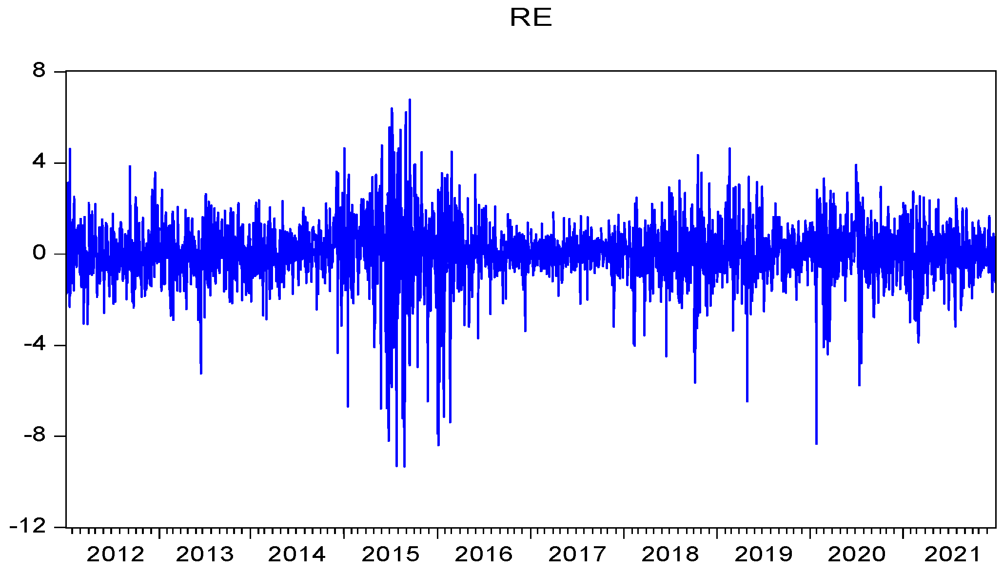
The real economy industry index is represented by nine types of CSI industry indexes other than the CSI financial index. These nine types of CSI industry indexes are the energy, material, information technology, manufacturing, medical, telecom, consumer goods, selective consumer and public utilities industries. Similarly, the daily closing price of the Real Economy Industry index from January 2012 to December 2021 is also selected as the sample data. The return is calculated as:

$${\mathrm{r}}_{\mathrm{i},\mathrm{t}}=100\left({\mathrm{lnP}}_{\mathrm{i},\mathrm{t}}-{\mathrm{lnP}}_{\mathrm{i},\mathrm{t}-1}\right)$$

(15)

where P_t is the closing price at time t.

4.2. Result of Time Series Analysis

4.2.1. ADF Test

According to the constructed fintech index and the obtained CSI industry index, the time series of return is calculated. Figure 2 and Figure 3 are the sequence diagrams of the return series of fintech and the real economy, respectively. It can be seen that the return mainly fluctuates between −4 and 4, with obvious fluctuation aggregation characteristics. The change characteristic shows that Fintech does not conform to the characteristics of normal distribution.

Figure 4 is the return series of the real economy industries index. Most industry indexes have the same variation as the Fintech index, but the fluctuation range is smaller, between −2.5 and 2.5. The return series of selected real economy industries have the characteristics of volatility aggregation, which also shows that the real economy industries index does not accord with the characteristics of normal distribution.

Observing Figure 2, Figure 3 and Figure 4, we can also find that the return series of the Fintech index and the various real economy industry indexes fluctuate around the mean. The fluctuation of the return series is uneven; there are multiple peaks, and the positions of the peaks are relatively consistent. Especially in the period of 2015–2017, the abnormal fluctuations are particularly obvious for all industries as well. The reason can be explained by policy reform. During this period, China brought all the financial businesses of P2P Internet loan platforms under supervision, launched a special action to combat the crime of illegal fundraising, and investigated and dealt with more than 10,000 illegal cases, which led to great fluctuations in financial innovation services. At the same time, China also adjusted its industrial structure and encouraged scientific and technological innovation. A large number of entity enterprises made major changes in their strategic planning, resulting in the business performance fluctuating greatly. On the other hand, it can also be roughly inferred that there is a certain degree of correlation between Fintech and various real economy industries.

Due to the errors in graphical observation, it is necessary to understand the characteristics and stationarity of return series through descriptive statistical analysis and the ADF test before empirical research. The test results are shown in

Table 1. Results of descriptive statistics and ADF test.

Variable	Min	Max	Mean	Stdev	Skew	Kurtosis	J-B Test	ADF	Stable
Fintech	−9.41	7.57	0.00	1.64	−0.41	6.75	450.28 ***	−26.32 *	Yes
Real Econ.	−8.04	6.10	0.02	1.47	−0.40	6.14	478.13 ***	−26.09 *	Yes
Energy	−8.05	6.07	−0.04	1.39	−0.44	6.68	437.33 ***	−26.37 *	Yes
Material	−9.51	5.65	0.01	1.54	−0.57	6.69	455.71 ***	−26.37 *	Yes
Selective consumer	−9.34	4.73	0.04	1.52	−0.62	6.02	324.89 ***	−26.54 *	Yes
Consumer goods	−8.17	5.82	0.02	1.72	−0.31	5.20	160.24 ***	−27.23 *	Yes
IT	−9.84	6.58	0.04	2.06	−0.40	4.79	117.45 ***	−26.84 *	Yes
Medical	−7.05	4.78	0.05	1.63	−0.28	3.76	27.33 ***	−26.94 *	Yes
Telecom	−10.20	6.77	−0.04	2.06	−0.33	5.90	270.09 ***	−25.91 *	Yes
Public Uti.	−8.06	4.05	−0.02	1.01	−0.95	10.59	1867.48 ***	−28.08 *	Yes
Manufact.	−9.54	5.09	0.02	1.40	−0.66	8.09	843.01 ***	−26.79 *	Yes

Note: *, *** denote significant at confidence level of 1% and 10%, respectively; J-B stands for Jarque Bera statistics.

.

As shown in Table 1, the skewness of all the index series is negative and all the kurtosis values are greater than 3.0, indicating that the index series have the characteristics of asymmetry, and peak and thick tail. The values of J-B are far greater than 0, the null hypothesis of normal distribution is rejected, so all the index series do not obey the normal distribution.

At the confidence level of 1%, the absolute values of the ADF statistics are far greater than their critical values, rejecting the null hypothesis that there are unit roots. Therefore, all the index series have no unit root and are stable.

4.2.2. Granger Causality Test

After the index time series has passed the ADF stability test, we can judge the impact relationship between Fintech and the real economy through the Granger causality test. In order to draw a more accurate conclusion, we selected the lag periods from 1 to 8 for testing, and the test results are shown in

Table 2. Granger causality test of Fintech index and Real Economy index.

Null Hypothesis	Lags	F-Statistic	Prob.	Result
Fintech does not Granger cause RE	1	6.7582	0.0094 *	Reject
RE does not Granger cause Fintech	1	9.1337	0.0025 *	Reject
Fintech does not Granger cause RE	2	4.3756	0.0127 **	Reject
RE does not Granger cause Fintech	2	5.2415	0.0054 *	Reject
Fintech does not Granger cause RE	3	7.1633	9 × 10−5 *	Reject
RE does not Granger cause Fintech	3	4.2180	0.0055 *	Reject
Fintech does not Granger cause RE	4	6.2489	5 × 10−5 *	Reject
RE does not Granger cause Fintech	4	3.2788	0.0109 **	Reject
Fintech does not Granger cause RE	5	5.0928	0.0001 *	Reject
RE does not Granger cause Fintech	5	3.0986	0.0086 *	Reject
Fintech does not Granger cause RE	6	5.1886	3 × 10−5 *	Reject
RE does not Granger cause Fintech	6	2.7154	0.0125 **	Reject
Fintech does not Granger cause RE	7	5.5768	2 × 10−6 *	Reject
RE does not Granger cause Fintech	7	2.36461	0.0208 **	Reject
Fintech does not Granger cause RE	8	4.7075	1 × 10−5 *	Reject
RE does not Granger cause Fintech	8	1.9797	0.0453 **	Reject

Note: *, ** denote significant at the confidence level 1% and 5%, respectively.

.

From the perspective of statistical causality, it is found that the Granger causality between fintech and the real economy under daily data is significantly bidirectional. That is, fintech is the Granger cause of the real economy, and the real economy is also the Granger cause of fintech at the confidence level 5%. This shows that there is a relationship of mutual influence and promotion between the two.

4.2.3. ARCH Effect Test

The Ljung–BoxQ statistic is used to investigate whether there is auto-correlation in Fintech, Real Economy, and CSI industries index series. The results of fintech return square series and the CSI industries index return square series are shown in

Table 3. Auto-correlation test.

Variable	$\mathbf{Q}\left(6\right)$	${\mathbf{Q}}^2\left(6\right)$	$\mathbf{Q}\left(36\right)$	${\mathbf{Q}}^2\left(36\right)$
Fintech	13.028 **	7.043	42.082 **	36.218
Real Economy	7.331	19.652 ***	36.149	51.165 **
Energy	8.072	24.140 ***	22.969	36.025
Material	9.659 ***	13.930 **	41.542 ***	53.176 **
Selective consumer	8.214	19.576 ***	29.039	52.037
Consumer goods	4.235	31.335 ***	28.525	59.509 ***
IT	7.812	15.009 **	41.590	58.534 ***
Medicine	0.538	43.541 ***	23.969	87.534 ***
Telecom	4.854	15.760 **	53.274 **	55.960 **
Public utilities	11.184 *	4.336	49.727 *	10.268
Manufacture	11.412 *	9.247	34.707	47.446 *

Note: Q(k) and Q²(k) represent whether the auto-correlation coefficients of return series and return square series lag 1–36 orders are combined to 0, respectively. *, **, *** denote significant at the confidence level 1%, 5% and 10%, respectively.

.

The Q(k) statistic shows that there is a certain weak auto-correlation between the Fintech return series and the CSI index return series, and the Q²(k) statistic shows that the Fintech return series and the CSI index return series have conditional heteroscedasticity.

In order to eliminate the auto-correlation and heteroscedasticity of model estimation, the GARCH model is selected to fit the edge distribution. The ARCH effect of each return series is tested to judge whether the GARCH model can be applied.

The results in

Table 4. ARCH effect test.

Variable	ARCH-LM(2)	ARCH-LM(4)
Fintech	3.892 ***	2.922 ***
Real Economy	19.122 ***	11.826 ***
Energy	8.122 ***	6.386 ***
Material	24.558 ***	12.663 ***
Selective consumer	68.744 ***	35.605 ***
Consumer goods	19.916 ***	15.528 ***
IT	15.637 ***	8.132 ***
Medicine	13.529 ***	13.879 ***
Telecom	9.791 ***	6.852 ***
Public Utilities	4.458 ***	3.394 ***
Manufacture	6.66 ***	4.054 ***

*** denote significant at the confidence level 10%.

show that both the Fintech return series and CSI industries index return series have a significant ARCH effect at the confidence level of 1%, which shows that it is applicable to use the GARCH model to fit the edge distribution.

4.3. Result of Edge Distribution

Through the ADF test and the ARCH effect test, we also found that the return series of Fintech and real economy industries do not obey the normal distribution and have the characteristics of peak and thick tail. Based on this, in order to better characterize the properties of time series, this paper constructs a GARCH (1,1) model under t distribution.

In

Table 5. Parameter estimation results of GARCH (1,1).

Variable	${\mathsf{\alpha }}_0$	${\mathsf{\alpha }}_1$	${\mathsf{\beta }}_1$	${\mathsf{\alpha }}_{\mathbf{1}}$$\mathbf{+}{\mathsf{\beta }}_{\mathbf{1}}$
Fintech	0.123 *	0.05 **	0.911 ***	0.961
Energy	0.153 *	0.059 **	0.869 ***	0.928
Material	0.11 **	0.073 ***	0.888 ***	0.961
Selective consumer	0.125 **	0.068 **	0.883 ***	0.951
Consumer goods	0.172 *	0.06 **	0.884 ***	0.944
IT	0.219 *	0.05 **	0.9 ***	0.95
Medicine	0.077 **	0.054 ***	0.919 ***	0.973
Telecom	0.148 **	0.056 ***	0.915 ***	0.971
Public Utilities	0.038 **	0.047 **	0.917 ***	0.964
Manufacture Ind.	0.092 **	0.054 **	0.903 ***	0.957

*, **, *** denote significant at the confidence level 1%, 5% and 10%, respectively.

, α₁ represents the coefficient of the ARCH term, namely the square lag term of residual error. β₁ represents the GARCH term, that is, the coefficient of the lag term of the conditional variance itself.

It can also be observed that all parameters of GARCH (1,1) are significant at the 10% confidence level, and the estimated values of each parameter are significantly positive, meeting the requirements of non-negative conditional heteroscedasticity. From the perspective of estimating the value of parameters, the α value represents the impact of external shocks on the fluctuation of the return series, and the β value represents the impact of early-stage fluctuation of the return series on later-stage fluctuation. Therefore, it can be found that the fluctuation of the return series of fintech and real economy industries is relatively less affected by external factors, and the fluctuation of the return series is closely related to its own early performance. The relationship between Fintech and the return series of various industries in the real economy α₁ + β₁ is close to 1, indicating that the volatility of return has strong sustainability. In addition, the ARCH term and GARCH term coefficients of each return series are significantly positive at the 95% confidence level, and α₁ + β₁ is less than 1, meeting the requirements of model stability.

4.4. Results of Dependent Structure by R-Vine Copula Model

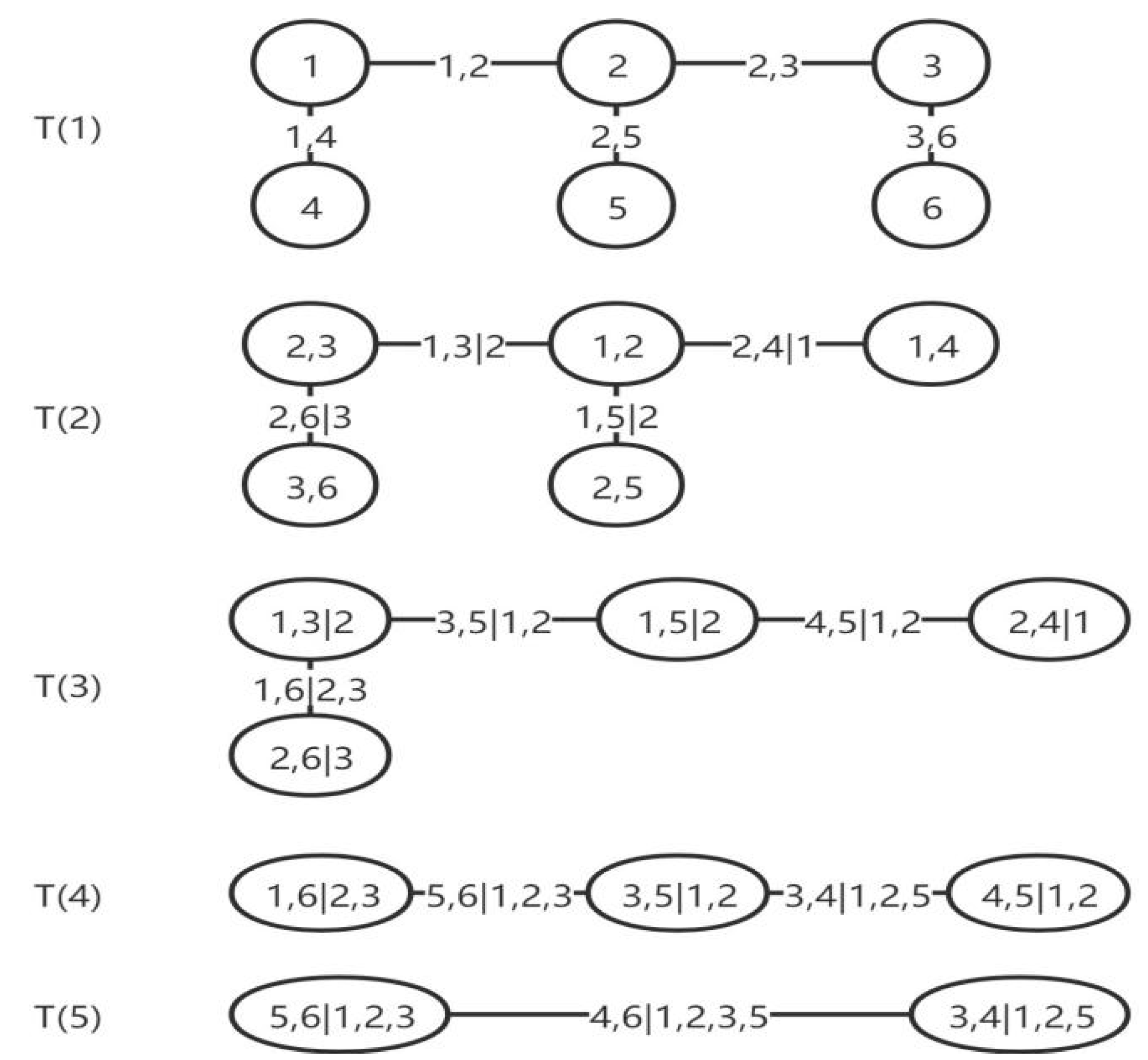
To more intuitively and comprehensively express the dependent structural relationship between Fintech and various industries of the real economy, this paper analyzes the first four trees of the R-vine model. The standardized residual sequences after probability integral transformation are firstly fitted, the R-vine model is constructed and the parameters are estimated to judge the dependency relationship and dependency structure between Fintech and various industries of the real economy. After selecting the optimal Pair copula function based on AIC and BIC information criteria, the tail dependence among industries is analyzed. The strength of the dependence is compared by the Kendall τ of the Copula function.

Figure 5, Figure 6, Figure 7 and Figure 8 show the first four trees of the R-vine. The abbreviations in the box are the industries, where FC represents financial technology, CO represents consumer industry, Ma represents material industry, EN represents energy industry, ME represents medical industry, PUB represents public utility industry, Ind represents manufacturing industry, Inf represents information industry, Tele represents telecommunications industry and SE represents other selective consumer industry. The connection between the box and the middle of the box shows the form of multivariate Copula function, and the value in parentheses is the Kendall τ of the two markets.

It can be seen from the figures that Fintech is located in the center of overall network connection and has a certain degree of correlation with various industries, which shows that the financial industry has established extensive correlation with industries such as materials and information technology. It not only shows that financial technology products and services can help the development of real economy industry, but also makes the spread of financial risks more complex and hidden. In addition, the core position of financial technology also shows that financial technology is an important medium for transmitting risks.

The R-vine estimation results show that Fintech has a strong correlation with the manufacturing, material, public utilities and selective consumer industries. Among them, Fintech has the highest correlation with the manufacturing industry, whose Kendall τ value is 0.71, followed by the material industry, selective consumer industry and public industry. The medical and consumer industries are not closely connected with Fintech and are far away from the central node.

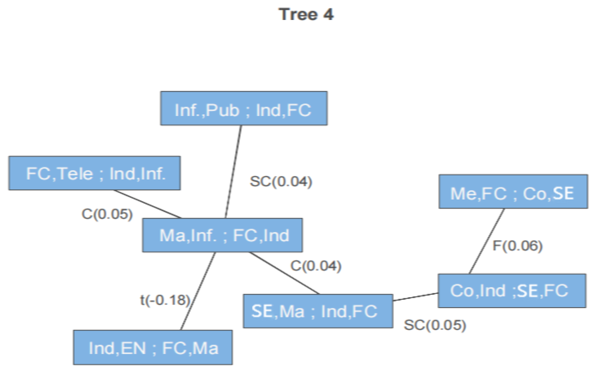
In the first tree in Figure 5, the telecommunication, public utilities, medical and energy industries constitute four separate branches, indicating that when extreme risks occur in these industries, they are often transmitted to other industries through Fintech products and services. In the second tree, Fintech and the manufacturing industry are located in the center, indicating that the manufacturing industry has a wide correlation. Compared with other real economy industries, the impact of the manufacturing industry is more profound. In addition, after adding industry, it can be found that Fintech and the information industry also have a strong correlation. Then the material and information industries were added to the center of the dependent structure, and the addition of material changed the basic form of the tree structure, so that the tree shape no longer shows the characteristics of four branches, but produces a sub center including the manufacturing industry, Fintech and information industry, showing that the information industry is highly related to public utilities, telecommunication and other industries. After the information industry is added to the center of the fourth tree, the tree shape returns to the four-branch structure similar to the first two trees. On the whole, there is a wide connection between Fintech and various industries of the real economy. Among them, Fintech, the manufacturing industry, the material industry and the information industry are highly related to other industries, and the dependent structure between them is more significant, while the manufacturing industry association relationship to the medical and other industries is relatively simple, showing the characteristics of strong independency.

The existence of tail dependence and the strength of the dependent relationship can judge whether there is extreme risk of infection among industries. The estimation of the first four trees of the R-vine is shown in

Table 6. Estimation results of R-vine Copula model.

R-Vine	Tree Structure	Type	Par	Par2	Kendall’s Tau	${\mathsf{\lambda }}_{\mathbf{U}}$	${\mathsf{\lambda }}_{\mathbf{L}}$
First tree	Ma,EN	t	0.80	6.20	0.60	0.41	0.41
	FC,Pub	t	0.79	3.04	0.58	0.52	0.52
	Inf,Tele	t	0.89	6.26	0.70	0.53	0.53
	Ind,Inf	t	0.87	8.00	0.67	0.45	0.45
	FC,Ma	t	0.88	3.92	0.69	0.60	0.60
	FC,Ind	t	0.90	4.02	0.71	0.63	0.63
	FC,SE	t	0.87	6.50	0.67	0.49	0.49
	SE,Co	t	0.78	12.12	0.57	0.23	0.23
	Co,Me	t	0.75	9.66	0.54	0.24	0.24
Second tree	FC,EN|Ma	SG	1.12	0.00	0.10	-	0.14
	Ind,Pub|FC	SJ	1.21	0.00	0.11	-	0.23
	Ind,Tele|Inf	SJ	1.20	0.00	0.10	-	0.22
	FC,Inf|Ind	t	0.25	6.79	0.16	0.06	0.06
	Ind,Ma|FC	SG	1.17	0.00	0.15	-	0.19
	SE,Ind|FC	SG	1.18	0.00	0.15	-	0.20
	Co,FC|SE	SC	0.08	0.00	0.04	0.00	-
	Me,SE|Co	F	2.52	0.00	0.26	-	-
Third tree	Ind,EN|FC,Ma	SG	1.06	0.00	0.05	-	0.07
	Inf,Pub|Ind,FC	N	−0.16	0.00	−0.10	-	-
	FC,Tele|Ind,Inf	SJ	1.09	0.00	0.05	-	0.11
	Ma,Inf|FC,Ind	G270	−1.13	0.00	−0.11	-	-
	SE,Ma|Ind,FC	t	0.09	10.37	0.06	0.01	0.01
	Co,Ind|SE,FC	J270	−1.02	0.00	−0.01	-	-
	Me,FC|Co,SE	F	1.23	0.00	0.13	-	-
Fourth tree	Inf,EN|Ind,FC,Ma	t	−0.28	7.29	−0.18	0.00	0.00
	Ma,Pub|Inf,Ind,FC	SC	0.08	0.00	0.04	0.00	-
	Ma,Tele|FC,Ind,Inf	C	0.00	0.00	0.05	-	0.00
	SE,Inf|Ma,FC,Ind	C	0.08	0.00	0.04	-	0.00
	Co,Ma|SE,Ind,FC	SC	0.10	0.00	0.05	0.00	-
	Me,Ind|Co,SE,FC	F	0.51	0.00	0.06	-	-

. There are 30 groups of correlations in total. In the column Type, t represents the two-dimensional t-Copula function, n represents the two-dimensional normal Copula function, G represents the two-dimensional Gumbel Copula function, SG represents the two-dimensional Gumble Copula function corresponding to 180 degrees of rotation, C represents the two-dimensional Clayton Copula function, f represents the Frank Copula function and j represents the Joe Copula function. The number after the letter represents the rotation angle. For example, G270 represents the Gumbel Copula function rotating 270 degrees. par is the parameter estimated by the pair–Copula function corresponding to each group of correlation, par2 is the degree of freedom of the pair–Copula function, Kendall’s τ is the rank correlation coefficient, and λ_U and λ_L represent the upper and lower tail correlation coefficients, respectively.

According to the estimation results of the R-vine copula model in Table 6, it can also be found that there is a general positive linkage between industries in the real economy, and this result is also consistent with the conclusion in the previous discussion.

In addition, in the estimation results of the R-vine Copula model, we observed a positive conditional dependence between Fintech, the medical industry and the consumer industry, which reflects that the medical industry and the consumer industry is relatively weak; they are not independent of each other, and extreme risk events in the field of Fintech can also have a negative impact on the medical industry and consumer industry through transmission between markets.

The model estimation results also show that there is a nonlinear dependence between Fintech and real economy industries. The Copula function forms of the first tree in the table are symmetrical t-Copula functions. Kendall’s τ value represents the unconditioned correlation coefficient between industries. It can be found that the upper and lower tail correlation coefficients show symmetrical characteristics, while the model forms of the second tree to the fourth tree are more diversified.

In the first tree, there is a significant positive correlation between Fintech and the manufacturing industry, material industry, public utility industry and selective industry, in which the rank correlation coefficient is above 0.5. Generally speaking, the higher the upper and lower tail correlation coefficient, the greater the possibility of market rise and fall synchronization, so the higher the possibility of risk spillover. Among them, the upper and lower tail correlation coefficient of Fintech and the manufacturing industry is the largest, indicating that the correlation between the two markets is high, and extreme risk is easily transmitted between the two markets. The upper and lower tail correlation coefficient of the selective industry and the consumer industry is the smallest; it shows that the industry relevance of the two industries is weak and the ability to resist extreme risks is relatively strong.

It can be observed that the correlation coefficient between the information technology and the telecommunication industry is high, which indicates that when extreme risks occur in Fintech and overflow to the information technology industry, it may also be transmitted to other industries. On the whole, the correlation coefficients between Fintech and various industries of the real economy are above 0.2, which shows that the real economy industry has weak awareness and ability to resist external extreme risks. When extreme risk events occur in Fintech or other real economy industries, it is easy to have a negative impact on other relevant industries. This feature also reflects the sensitivity and vulnerability of Fintech itself. When the real economy industry is impacted by extreme risk events, it has varying degrees of negative impact on the capital market and even whole financial markets.

The second tree in Figure 6 represents the conditional dependence with an industry as the conditional variable. The estimation results show that the correlation between industries is significantly weakened after introducing an industry as a conditional variable. There is a weak positive correlation between Fintech and the energy industry, IT industry and consumer industry, after excluding the influence of the manufacturing industry, material industry and selective industry, respectively. At the same time, the correlation between real economy industries is also weakened after excluding the influence of Fintech.

The rank correlation coefficient and upper and lower tail correlation coefficient of the third tree in Figure 7 and the fourth tree in Figure 8 tend to 0, which indicates that the more conditional industries are introduced, the weaker the correlation between industries. When extreme risks occur in an industry, risk transmission tends to spread among the three closely related industries; although the risks cannot be completely dispersed, its impact on other industries is limited.

It can be seen from the R-vine Copula model trees that Fintech occupies the central position of the dependent structure, which proves that Fintech has established a broad and profound correlation with the market, and the real economy industries with weak correlation are also linked by Fintech products and services. However, the improvement of the degree of correlation not only enhances the availability of financial products and services, but also has new risk threats that are difficult to prevent by the traditional risk prevention and control system. The establishment of this dependent structure provides a way for the spread of potential risks. While accelerating the spread of extreme risks, the degree of harm is further deepened. The tail risk estimation in the estimation results of the R-vine Copula model also shows this problem. The upper and lower tail correlation coefficient is significantly positive, indicating that the extreme risk of one industry increases the risk level of other industries.

In the R-vine Copula model, the correlation between Fintech and industries with large capital demand and relatively slow turnover speed, such as the manufacturing industry, IT industry and material industry, is higher, which further confirms that enterprises with a long capital chain and large capital demand are more closely related to the financial system; such enterprises are more sensitive to Fintech products and services than enterprises with a short capital chain. Fintech and the medical industry have developed in the fields of integration of medicine and medical resources, innovation of medical insurance products and financial services, but it has a low correlation with Fintech, so the impact of financial risk on the medical industry is also relatively limited. From a macro perspective, Fintech in the medical industry may help to reduce medical costs, optimize the allocation of medical resources and supplement the shortcomings of the existing social security and medical insurance systems. However, how Fintech products and services adapt to the market demand in the medical industry still needs to be further explored.

4.5. Result of Risk Spillover Effect

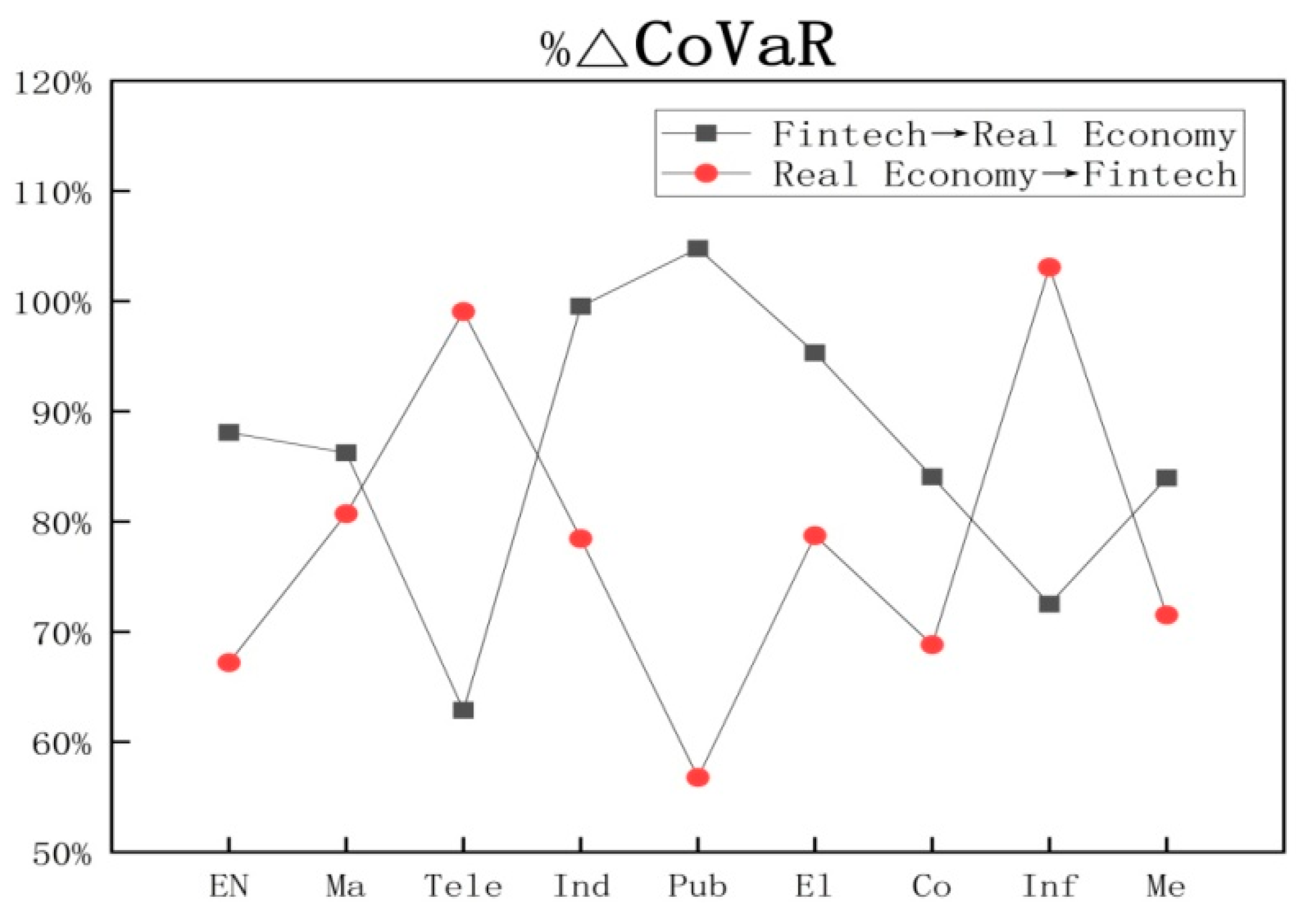
From the research results of the R-vine copula, it can be found that the dependences between Fintech and various industries of the real economy are different, but they have formed a wide range of correlation, indicating a strong risk transmission effect. VaR, CoVaR, ∆CoVaR and % ∆CoVaR are calculated to measure the two-way risk spillover effect. The CoVaR value is generally greater than 4, ∆ Covar is greater than 3 and the% ∆ Covar value is also more than 60%, which indicates that when extreme risks occur in Fintech, it is very likely to have a different degree of negative impact on industries of the real economy, and the risk spillover level is higher than the risk level of the real economy industry itself.

Table 7. Fintech risk spillover to industries in real economy.

Risk Spillover	VaR	CoVaR	$\mathsf{\Delta }\mathbf{CoVaR}$	$\mathbf{\%}\mathsf{\Delta }\mathbf{CoVaR}$
Fintech → Energy	3.68	4.42	3.25	88.09%
Fintech → Material	3.48	4.08	3.00	86.23%
Fintech → Selective consume	3.58	4.21	2.25	62.87%
Fintech → Consume	3.09	3.86	3.08	99.53%
Fintech → IT	3.30	4.15	3.45	104.79%
Fintech → Medicine	3.66	4.34	3.49	95.31%
Fintech → Telecom	4.24	5.10	3.57	84.05%
Fintech → Public Uti.	3.52	4.17	2.55	72.51%
Fintech → Manufacture	4.19	4.98	3.52	83.96%

shows the degree of risk spillover to various industries of the real economy when extreme risks occur in the Fintech industry at the 95% confidence level.

The estimation result is consistent with the correlation result of the R-vine Copula. Compared with other industries, Fintech has the strongest risk spillover level to the manufacturing industry, public utilities industry and selective industries. According to the empirical analysis results, it can be seen that there is a high correlation between the manufacturing industry and Fintech. Although the public utilities industry and selective industries have a weak relationship with Fintech, they are also vulnerable to extreme risk spillovers in Fintech due to their weak financial risk prevention ability.

Table 8. Risk spillover of industries in real economy to Fintech.

Risk Spillover	VaR	CoVaR	$\mathsf{\Delta }\mathrm{CoVaR}$	$\mathbf{\%}\mathsf{\Delta }\mathrm{CoVaR}$
Energy → Fintech	3.04	3.94	2.04	67.20%
Material → Fintech	3.07	3.96	2.48	80.71%
Selective consumer → Fintech	4.29	5.50	4.25	99.06%
Consumer → Fintech	2.73	3.28	2.14	78.45%
IT → Fintech	2.31	2.83	1.31	56.78%
Medicine → Fintech	3.11	4.11	2.45	78.73%
Telecom → Fintech	3.55	4.79	2.44	68.83%
Pub Uti. → Fintech	3.96	5.13	4.08	103.08%
Manuf. Ind. → Fintech	3.62	4.91	2.59	71.52%

shows the Risk Spillover degree to all industries of the real economy when extreme risks occur in the Fintech industries at the 95% confidence level. It can be seen that the CoVaR value is greater than 3, the ∆CoVaR value is above 2 and the % ∆CoVaR value is also greater than 50%, which indicates that various industries of the real economy are likely to have different degrees of negative impact on Fintech in the event of extreme risks, and the risk overflow level is higher than the risk level of Fintech itself. Compared with other industries, the telecommunication industry and IT industry have the strongest risk spillover effect on Fintech. This characteristic shows that Fintech is highly dependent on modern information technologies such as big data and cloud platforms. Risk events in related industries have a great negative effect on Fintech.

Figure 9, Figure 10 and Figure 11 show the comparisons of the risk spillover degree by CoVAR, ∆CoVaR and %∆CoVaR, respectively.

From the figures it can be seen that the risk spillover effect of extreme risks in Fintech on most industries of the real economy is relatively strong, while the CoVaR results of various industries of the real economy are relatively small, which has a slightly smaller impact than that caused by extreme risks in Fintech. This can also reflect that the concealment and harmfulness of financial risk contagion are strong, and the risk prevention ability and awareness of Fintech are also better than those of the real economy.

5. Discussion

5.1. Rationality of Methodology

5.1.1. Time Series Approach

Time series analysis is used to determine the long-term trend, periodic change, cyclic fluctuation and irregular change in the time series. According to the characteristics of risk spillover, it is obvious that the time series method is more appropriate in this paper, because the tail residual perturbation term of the time series equation can reflect the influence of factors changing with time.

The Granger causality test is conducted to judge the impact relationship between financial innovation and the real economy; the result shows that this is a positive relationship, which is consistent with the conclusions of other scholars such as Shin and choi [7] and Tian, Li, and Yang [8].

The GARCH model is used to get the tail conditional variance for the edge disruption in the Copula, because the time series of the Fintech index and real economy index have an ARCH effect with characteristics of peak and thick tail, and GARCH can interpret this phenomenon and the asymmetry well.

5.1.2. Deficiency of Copula

Copula is a function connecting multi-dimensional joint distribution and its edge distribution. It can completely describe the correlation structure between variables, and can also separate the edge distribution from the correlation structure. In addition, one of the two can be selected independently, which greatly reduces the difficulty of obtaining the multivariable joint distribution function. Saraji, Karimalis et al. [16,19] indicated that the correlation structure between financial markets is closely related to risk management.

Although the copula function is very convenient in investigating correlation and edge distribution, it faces great challenges in dealing with high-dimensional structures. Therefore, the vine copula method came into being by scholars such as Joe, Li, Nikoloulopoulos, Sriboonchitta, Kosheleva, Nguyen, Alanazi, Bedford, Daneshkhah, Wilson, Zhu, Kurowicha, and so on [20,21,22,23,24].

5.1.3. Advantages of R-Vine Copula

The vine copula is a multivariate dependence model, which is composed of a collection of bivariate copulas consisting of specific underlying graphical structure. The most often used are the C-vine copula, D-vine copula and R-vine copula. We use the R-vine copula for this study, because it is not only practical for decomposing a high dimension copula into multiple bivariate copulas, but also has the flexibility to describe the conditional dispersion effect of nodes according to the dependence intensity of the market [21,24,25].

In modeling of the R-vine, the choice of vine structure is to construct a continuous tree by capturing the largest correlation in the underlying tree. However, this does not guarantee that the best vine structure is generated. This paper intends to improve the RVM with reference to the maximum spanning tree (MST) method proposed by Brechmann et al. [42], and then determine the decomposition structure of the R-vine model. The algorithm is appropriately improved according to the sampling sequence. The idea is to search an R-vine–copula from an initial vine structure, which better represents the rattan data with two common sampling sequences, making the R-vine-copula model more suitable for the data dependency structure.

After obtaining the optimized copula function, given a certain confidence level, the cumulative probability of CoVaR can be obtained according to the AIC principle. Next, the cumulative probability is inversely substituted into the edge distribution function, then the risk spillover CoVaR can be obtained by solving the inverse edge distribution function [19,43].

Therefore, it can be concluded from the above discussion that the combined R-vine–Copula model that we have constructed is reasonable.

5.2. Managerial Implication

With the development of economic integration, the relevance to all walks of life is becoming higher and higher. Therefore, fintech has a greater impact on the entire economic system. From the analysis of the copula edge distribution and R-vine dependent structure, it is found that fintech and the real economy promote each other; risks also spread across them and spillover effects occur. The contribution of different industries to the systematic risk of the market is significantly different with the characteristics of asymmetry.

Therefore, this study provides an important reference for how to diversify the systemic fintech risks, so as to prevent them from having an impact on the real economy. It is of great practical significance to further explore the impact of fintech innovation on systematic financial risks, make rational use of financial technology to promote long-term healthy economic development, and pay attention to the possible spillover risk caused by excessive innovation of financial technology.

5.3. Limitation and Future Work

In the study, we found that there are extreme risks in the time series, but the existence of the extreme risk effect and its impact on the whole system were not taken into account in our model construction. In order to make the model more comprehensively reveal the complex structure of various industries, we will add an extreme value effect in future research, so as to analyze the risk transmission path and dispersion effect under extreme risk conditions, making the model more accurate in describing the risk.

6. Conclusions

The correlation structure of the R-vine Copula model shows that there is a positive correlation between Fintech and various industries of the real economy, and there is also a general positive linkage. The Fintech industry is located in the central position of the dependent structure. The Fintech industry has the highest rank correlation coefficient with the manufacturing industry and material industry. In addition, we have observed that there is a positive conditional dependence between the Fintech industry, medical industry and consumer industry, which reflects that the correlation is relatively weak. Extreme risk events in Fintech can also have a negative impact on the medical industry and consumer industry.

The estimation results of the R-vine Copula model reflect that there is a nonlinear dependence between Fintech and the real economy. The upper and lower tail correlation coefficients of the first tree show the symmetrical characteristics, indicating that there is the possibility of simultaneous rise and fall between Fintech and the real economy industries.

CoVaR analysis shows that extreme risk events in Fintech and various industries of the real economy have different degrees of negative impact on each other, and the risk spillover level is relatively high. When extreme risks occur in Fintech, the manufacturing industry is also subject to a high degree of risk impact. Although the public utilities industry and selective industries have a weak relationship with Fintech, they are also vulnerable to extreme risk spillovers from Fintech due to their weak financial risk prevention ability.

Based on the above conclusions, this paper believes that under the trend of the increasingly extensive application of Fintech products and services, the dominant position of the real economy needs to be further strengthened. In order to give full play to the real value of Fintech, we must strengthen the dominance of the real economy and realize the goal of Fintech to serve the development of the real economy. In addition, the ability of the real economy industry to prevent and resolve financial risks needs to be improved. Before the outbreak of financial risks, it can effectively identify and respond to risks, not only making full use of the value brought by Fintech products and services, but also effectively avoiding risk accumulation and risk infection.

References

1. Li, J. Thoughts on internet finance. Manag. World 2015, 31, 1–7. [Google Scholar]
2. Lu, Y. Industry 4.0: A survey on technologies, applications and open research issues. J. Ind. Inf. Integrat. 2017, 6, 1–10. [Google Scholar] [CrossRef]
3. Zilgalvis, P. The need for an innovation principle in regulatory impact assessment: The case of finance and innovation in European. Policy Internet 2015, 6, 377–392. [Google Scholar] [CrossRef]
4. Gennaioli, N.; Shleifer, A.; Vishny, R. Neglected risks, financial innovation and financial fragility. J. Financ. Econ. 2012, 104, 452–468. [Google Scholar] [CrossRef] [Green Version]
5. Chen, X.H.; Teng, L.; Chen, W. How does fintech affect the development of the digital economy? Evidence from China. N. Am. J. Econ. Financ. 2022, 61, 101697. [Google Scholar] [CrossRef]
6. Chen, X.H.; Yan, D.; Chen, W. Can the digital economy promote fintech development? Growth Chang. 2021, 53, 221–247. [Google Scholar] [CrossRef]
7. Shin, Y.J.; Choi, Y. Feasibility of the fintech industry as an innovation platform for sustainable economic growth in Korea. Sustainability 2019, 11, 5351. [Google Scholar] [CrossRef] [Green Version]
8. Tian, X.; Li, R.; Yang, G. The impact of fintech on the development of real economy—An empirical analysis based on the dual path of financial innovation. Guangdong Soc. Sci. 2021, 17, 5–15. [Google Scholar]
9. Sun, P.; Zhang, R. Whether financial innovation promotes or hinders economic growth: A panel analysis from the perspective of technological progress. Mod. Econ. Sci. 2012, 33, 26–35. [Google Scholar]
10. Thorsten, B.; Tao, C.; Chen, L. Financial innovation: The bright and the dark sides. J. Bank. Financ. 2016, 72, 28–51. [Google Scholar]
11. Lee, I.; Yong, J.S. Fintech: Ecosystem, business models, investment decisions, and challenges. Bus. Horiz. 2018, 61, 35–46. [Google Scholar] [CrossRef]
12. Rafal, S.; Daniel, P. Conditional correlation coefficient as a tool for analysis of contagion in financial markets and real economy indexes based on the synthetic ratio. Proc. Soc. Behav. Sci. 2016, 220, 452–461. [Google Scholar]
13. Vucinic, M.; Luburic, R. Fintech, risk-based thinking and cyber risk. J. Cent. Bank. Theo. Pract. 2022, 11, 27–53. [Google Scholar] [CrossRef]
14. Chen, R.; Chen, H.; Jin, C.; Wei, B.; Yu, L. Linkages and spillovers between internet finance and traditional finance: Evidence from China. Emerg. Market. Financ. Trad. 2020, 56, 1196–1210. [Google Scholar] [CrossRef]
15. Namchoochai, R.; Kiattisin, S.; Darakorn Na Ayuthaya, S.; Arunthari, S. Elimination of fintech risks to achieve sustainable quality improvement. Wirel. Person. Comm. 2020, 115, 3199–3214. [Google Scholar] [CrossRef]
16. Saraji, M.K.; Streimikiene, D.L.; Kyriakopoulos, G.L. Fermatean fuzzy critic-copras method for evaluating the challenges to Industry 4.0 adoption for a sustainable digital transformation. Sustainability 2021, 13, 9577. [Google Scholar] [CrossRef]
17. Yu, C.; Wang, X. Empirical test of financial innovation on high-quality economic development. Stat. Decis. Making. 2021, 37, 88–92. [Google Scholar]
18. Lin, J.; Zhao, H. Research on risk spillover effect of Shanghai, Shenzhen and Hong Kong Stock Markets—Based on time-varying ΔCoVaR Model. Sys. Eng. Theory Pract. 2000, 40, 1533–1544. [Google Scholar]
19. Karimalis, E.N.; Nokimos, N.K. Measuring systemic risk in the european banking sector: A copula Co-VaR approach. Eur. J. Financ. 2018, 24, 944–975. [Google Scholar] [CrossRef] [Green Version]
20. Joe, H.; Li, H.J.; Nikoloulopoulos, A.K. Tail dependence Functions and Vine Copulas. J. Multivariat. Anal. 2010, 101, 252–270. [Google Scholar] [CrossRef] [Green Version]
21. Sriboonchitta, S.; Kosheleva, O.; Nguyen, H.T. Why are vine copulas so successful in econometrics? Int. J. Uncertain Fuzz. 2015, 23, 133–142. [Google Scholar] [CrossRef]
22. Alanazi, F.A. A mixture of regular vines for multiple dependencies. J. Prob. Stat. 2021, 5559518, 1–15. [Google Scholar] [CrossRef]
23. Bedford, T.; Daneshkhah, A.; Wilson, K.J. Approximate uncertainty modeling in risk analysis with vine copulas. Risk Anal. 2016, 36, 792–815. [Google Scholar] [CrossRef] [PubMed] [Green Version]
24. Zhu, K.L.; Kurowicka, D.; Nane, G.F. Common sampling orders of regular vines with application to model selection. Comput. Stat. Data Anal. 2020, 142, 106811. [Google Scholar] [CrossRef]
25. Schepsmeier, U. A goodness-of-fit test for regular vine copula models. Econom. Rev. 2019, 38, 25–46. [Google Scholar] [CrossRef] [Green Version]
26. Kim, D.; Kim, J.M.; Liao, S.M.; Jung, Y.S. Mixture of D-vine copulas for modeling dependence. Comput. Stat. Data Anal. 2013, 64, 1–19. [Google Scholar] [CrossRef]
27. Nikoloulopoulos, A.K.; Joe, H.; Li, H. Vine copulas with asymmetric tail dependence and applications to financial return data. Comput. Stat. Data Anal. 2012, 56, 3659–3673. [Google Scholar] [CrossRef]
28. Karakas, A.M.; Demir, A.; Calik, S. Vine copula approach for modeling dependence of commodity and stock markets. J. Stat. Manag. Sys. 2022, 25, 1877904. [Google Scholar]
29. Autchariyapanitkul, K.; Piamsuwannakit, S.; Chanaim, S.; Sriboonchitta, S. Optimizing stock returns portfolio using the dependence structure between capital asset pricing models: A vine copula-based approach. Causal Infer. Econom. 2016, 622, 319–331. [Google Scholar]
30. Czado, C.; Schepsmeier, U.; Min, A. Maximum likelihood estimation of mixed C-vines with application to exchange rates. Stat. Model. 2012, 12, 229–255. [Google Scholar] [CrossRef] [Green Version]
31. Zhang, Z.; Zhang, T. Risk correlation measurement of major global stock markets—Based on semi Parametric C-Vine Copula Model. Financ. Rev. 2018, 10, 23–34. [Google Scholar]
32. Reboredo, J.C.; Ugolini, A. Downside/upside price spillovers between precious metals: A vine copula approach. N. Am. J. Econ. Financ. 2015, 34, 84–102. [Google Scholar] [CrossRef]
33. Guo, W. Structural deleveraging and systemic risk spillovers of financial institutions: Promotion or inhibition? J. Centr. Univ. Financ. Econ. 2020, 40, 26–41. [Google Scholar]
34. Zhang, D.L.; Yan, M.L.; Tsopanakis, A. Financial stress relationships among euro area countries: An R-vine copula approach. Eur. J. Financ. 2018, 24, 1587–1608. [Google Scholar] [CrossRef]
35. Heston, S.L.; Nandi, S. A Closed-form GARCH option valuation model. Rev. Financ. Stud. 2000, 13, 585–625. [Google Scholar] [CrossRef]
36. Ji, H.; Wang, H.; Liseo, B. Portfolio diversification strategy via tail-dependence clustering and ARMA-GARCH vine copula approach. Aust. Econ. Pap. 2018, 57, 265–283. [Google Scholar] [CrossRef]
37. Patton, A.J. Modeling asymmetric exchange rate dependence. Int. Econ. Rev. 2006, 47, 527–556. [Google Scholar] [CrossRef]
38. Sklar, A. Fonctions de repartition an dimensions et Leurs Marges. Publ. Inst. Stat. Univ. Paris 1959, 8, 229–231. [Google Scholar]
39. Hernandez, J.A.; Hammoudeh, S.; Nguyen, D.K. Global financial crisis and dependence risk analysis of sector portfolios: A vine copula approach. Appl. Econ. 2017, 49, 2409–2427. [Google Scholar] [CrossRef] [Green Version]
40. He, M.; Li, H. Dependence structure and extreme risk spillover among global stock markets: Financial complexity analysis based on Rattan Copula. Manag. Rev. 2020, 32, 102–110. [Google Scholar]
41. Dißmann, J.; Brechmann, E.C.; Czado, C. Selecting and estimating regular vine copula and application to financial returns. Comput. Stat. Data Anal. 2013, 59, 52–69. [Google Scholar] [CrossRef] [Green Version]
42. Brechmann, E.C.; Schepsmeier, U. Modeling dependence with C- and D-vine copulas: The R-package CD vine. J. Stat. Softw. 2013, 52, 1–27. [Google Scholar] [CrossRef] [Green Version]
43. Jiang, K. Research on financial risk spillover and its prevention in real estate industry—Analysis based on time-varying copula CoVaR model. Price Theory Pract. 2020, 40, 87–91. [Google Scholar]
Figure 1. 6-dimensional R-vine structure.
Sustainability 14 07818 g001
Figure 2. Return series of Fintech index.
Sustainability 14 07818 g002
Figure 3. Return series of Real Economy index.
Sustainability 14 07818 g003
Figure 4. Return series of industry index in real economy.
Sustainability 14 07818 g004
Figure 5. The first tree of R-vine.
Sustainability 14 07818 g005
Figure 6. The second tree of R-vine.
Sustainability 14 07818 g006
Figure 7. The third tree of R-vine.
Sustainability 14 07818 g007
Figure 8. The fourth tree of R-vine.
Sustainability 14 07818 g008
Figure 9. Comparison of risk spillover effect by CoVaR.
Sustainability 14 07818 g009
Figure 10. Comparison of risk spillover effect by ∆CoVaR.
Sustainability 14 07818 g010
Figure 11. Comparison of risk spillover effect by %∆CoVaR.
Sustainability 14 07818 g011