Simulation Analysis of a Double Auction-Based Local Energy Market in Socio-Economic Context

Abstract

Local energy markets (LEMs) use online platforms and smart grid technologies to incentivize and coordinate a local supply of spatially-distributed renewable energy resources, which may not be directly controllable by power system operators. Socio-economic values are increasingly noted as prominent motivations for expected LEM users, but socio-economic aspects of user decision-making or market outcomes are not considered in current LEM mechanism design analyses. Here, agent-based simulation is used to analyze expected socio-economic outcomes from LEM operation under a double-sided auction with uniform pricing. The environment is modeled as a virtual LEM platform, operating independently from the underlying power grid. Socio-economic market inputs are produced by income-preference heterogeneous agents, and market outcomes are evaluated by two key socio-economic metrics: energy affordability, and market access. When LEM prices are not restricted to a common range considered by all agents (e.g., between external retail market prices), access disparities may arise; LEM price restriction addresses consumer disparities, but energy affordability gaps are expected to remain. The magnitude of affordability gaps is notably reduced, and bill assistance programs may eliminate remaining gaps, but a mechanism that efficiently realizes socio-economic standards for energy affordability may also reduce expected LEM operation costs. Remaining research gaps are noted, and LEM support for equitable and sustainable energy infrastructure is emphasized.

1. Introduction

Electrical power grids which rely on centralized, fossil fuel-based energy generation currently face the challenge of safely and sustainably integrating renewable energy sources at a sufficiently large scale to support climate change adaptation and mitigation efforts. At the same time, centralized energy systems face challenges regarding operational resilience, and the production of equitable environmental and socio-economic outcomes for local communities. For example, even if we limit our scope to metropolitan areas just within the United States, we still find tens of millions of households with severely unaffordable energy costs [1].

Distributed energy systems (DES) have emerged through recent decades as a promising approach to energy infrastructure development centered around spatially and organizationally distributed renewable energy resources (RERs) for energy generation and storage. Local-level “microgrid” energy systems are a common focus in DES engineering research; these systems may integrate local-scale renewable energy supply into the “edges” of a power grid and may be coordinated to provide grid services such as local-level load balancing [2,3]. In DES, local energy markets (LEMs) have been proposed as mechanisms of incentivization and coordination for an expected DES power supply base consisting of a non-trivial amount of renewably-sourcedd energy supplied by spatially distributed local generators. In microgrid scenarios especially, these local generators are often called “prosumers”—or energy consumers which utilize renewable energy resources (RERs, such as solar PV panels) to offset their energy demand, and may produce surplus energy for LEM sale. For organizational simplicity, we refer to prosumers strictly as energy sellers in this study; however, in real-world systems, their role may change dynamically across time between buyer and seller. A variety of LEM mechanism designs have been proposed, largely consisting of direct optimization and game theoretic approaches [3,4,5].

In power grids which are equipped for bi-directional power transmission, and feature greater path redundancy than traditional systems (e.g., microgrids with peer-to-peer power networks), LEMs are expected to enable solutions to energy system carbon emissions, and to grid stability issues posed by renewable energy transition, while also improving local-level economic and “equity” outcomes produced by energy infrastructure operations. On an LEM platform which is physically connected to an underlying power system, LEM settlement may help set optimization constraints for power distribution locally. The “virtual” LEM, on the other hand, is essentially a marketplace for the trade of “energy credits”, which utility customers may purchase to offset their expenses from energy exchange in the current, centralized utility grid. A virtual LEM may run in parallel to retail energy markets, which often provide a wide range between retail sale prices for consumers, and retail purchase prices for prosumers with net energy supply. Nearly all real-world DES are currently structured around virtual LEMs; but while some LEMs restrict potential prices to this range, many LEM designs do not.

The LEM represents a critical vector of engagement between DES and the surrounding community, and a growing number of experimental works suggest that the socio-economic impacts of LEM operation are a strong factor in participation motivations for expected users [6,7,8,9]. Overall, the socio-economic impacts of LEM mechanisms on local households can be well-expected to impact community and user engagement with the platform. However, socio-economic outcomes are largely unconsidered in LEM design analysis, and socio-economic factors in user behavior are not currently modeled. Effective simulation-based modeling and analysis of influential socioeconomic factors in “virtual” LEM outcomes is emphasized as the primary research scope of the current work.

A key barrier to the assessment of expected socio-economic impacts lies in the modeling of software-based user agents which interact with the marketplace on behalf of users. In system implementations, either agents’ behavior is fully determined by user input, or else agents act autonomously on behalf of users while considering user preference inputs (e.g., price constraints, and level of preference for local, renewable energy) [10]. Users’ preference for own-economic value maximization is well-represented in current agent modeling [11]. Additional user inputs regarding preferences and bidding limits, for example, are strongly related to external individual and socio-economic conditions, but are not modeled.

The impacts of socio-economic inputs to the LEM are explored in this work using agent-based modeling. The described agent modeling includes household income distribution, economic rationality constraints, and value preferences as expected influential socio-economic input factors. In the modeling, these factors play key roles in defining the range of market strategies that an agent considers, and in producing behavioral reinforcement from market outcomes. Single-parameter utility models are defined which represent own-economic value (cost savings for consumers, and sales profits for prosumers), and “additional” value preferences under which value is placed on LEM supply due to the expected environmental and/or socio-economic benefits from its generation, sales, or use. A “preference parameter” mediates the influence of value types on consumer utility. A metric-based approach is taken to assessing socio-economic outcomes in the presented work. Two key socio-economic metrics are described and evaluated: energy affordability, and relative market access. Both are described in Section 2.6.

The Brooklyn Microgrid project is an increasingly well-known virtual LEM implementation [10]. It uses a uniform-price double-sided auction (UDA) mechanism to produce market settlement at discrete time intervals. Auction-based approaches are predominant in LEM mechanism design [4,12,13,14], but the expected socio-economic impacts of operating consumer-facing energy infrastructure via auction on local communities has not been well-studied. On the other hand, current retail energy markets generally provide full and equal access to the energy demand of connected utility customers, but often produce conditions of energy poverty among low-income households. For example, well over a million households in New York City alone experience energy costs over 50% greater, by proportion of household income, than the current energy affordability threshold of 6% adopted by the City of New York [15]. Consistent with [16], simulation environment parameters and LEM modeling in the current work represent the Brooklyn Microgrid and the surrounding area in 2019 (see Section 2.1). The presented work considers a multi-part research question, with each part answered via simulation experiment results analysis:

• How may socio-economic outcomes from LEM operation differ from current retail energy market outcomes, under a UDA mechanism? Specifically, can uniform market access be maintained under LEM operation? To what extent may local energy affordability issues be addressed? How may the range of allowed bidding and asking prices impact LEM outcomes?

2. Methodology

After simulation environment and agent parameters have been initialized, a simulation follows the execution loop noted in Figure 1. Agents representing LEM platform user households are modeled and initialized as shown in Section 2.2, Section 2.3 and Section 2.4 Households are assumed to be physically connected to the underlying power grid, and may access a retail energy market maintained by power grid operators. The LEM simulation has a “hub and spoke” network topology, in which each agent solely interacts with retail and local markets, solely via the modeled LEM platform.

In the current work, NetLogo is used to implement an agent-based simulation of a virtual LEM platform, which is modeled after the LEM utilized in the Brooklyn Microgrid. The underlying power system is not modeled, and agents’ energy supply and demand quantities are taken as a variable parameter in simulation experiments Experiments are conducted using the BehaviorSpace package for NetLogo, and simulation results for each experiment are analyzed via R scripts. Simulation environment modeling, including income distribution and energy markets, is described in Section 2.1; experiments are detailed in Section 3.

At each simulation step, agents select market strategies (bid or ask prices $S{\prime }_t$) via reinforcement learning and submit market quantity and strategy data to the marketplace. At each step, initial market quantities $Q_{0,t}= \{D_i+G_i: i \in I\}$ indicate consumer demand and prosumer supply, depending on agent “type” $C_i \in \{0, 1\}$ for a given agent $i \in I$. Market settlement is described in Section 2.1, and Section 2.4 describes agent-level parameter initialization. All symbols and parameters are described in the following sections, as they are presented. Parameter and symbol reference is provided in the Glossary, which is located in Section 6. Key simulation parameters are presented in Table 6, while Table 7 summarizes the data used to compute and describe simulated market settlements. In

Table 1. Overview of key abbreviated terms used in the current and previous sections.

Other Abbreviated Terms
Acronym	Name	Description
DES	Distributed energy system	Energy system which is decentralized, but feature some level of inter-connection; a number of localized microgrids connected to a main, regional energy grid is an example of DES; often characterized by RER
RER	Renewable energy resource	Device used for renewable energy generation, storage, etc. These may include, e.g., solar PV panels, wind turbines, battery storage, or electric vehicles.
LEM	Local energy market	Virtual platform to coordinate local-scale energy distribution; often a peer-to-peer network or a centralized auction platform for local utility customers
UDA	Uniform double-sided auction	A double-sided auction with a uniform market-clearing price, merit-order supply allocation, and a closed order book. Double-sided auctions are a class of auction commonly used to produce efficient allocations of private goods.

below, general abbreviations are noted which are used throughout the text.

After local market settlement, allocation quantities$Q_{loc,t }$and transaction prices$P_{loc,t}$ are collected for each agent, and the retail market is settled as described in Section 2.1. All remaining consumer demand is purchased from the main grid at the retail price $p_{ret}$, and all remaining prosumer supply is sold to the main grid at the feed-in tariff price $p_{fit}$. Based on study scope, static retail prices are assumed.

Retail and local market results data are then returned to agents, as shown in Figure 1. Based on market outcomes and individualized value functions, agents update their learning model states in preparation for the next simulation step. Agent behavior is described in Section 2.5. Data on market transactions and agent states are collected at the end of each step, which are used to calculate results analysis metrics (Section 2.6).

Sufficient power supply is assumed locally, and power grid stability is assumed regardless of prosumer behavior. At the same time, prosumers are modeled without consideration for storage resources; the impact of battery capacity, charge state, and supply scheduling efficiency, for example, may be considered in future work. Agents are also assumed to have perfect prediction for their own supply and demand at each time step. Local energy supply is assumed to be generated by prosumer households utilizing sustainably-sited residential-scale solar PV systems without energy storage capacity.

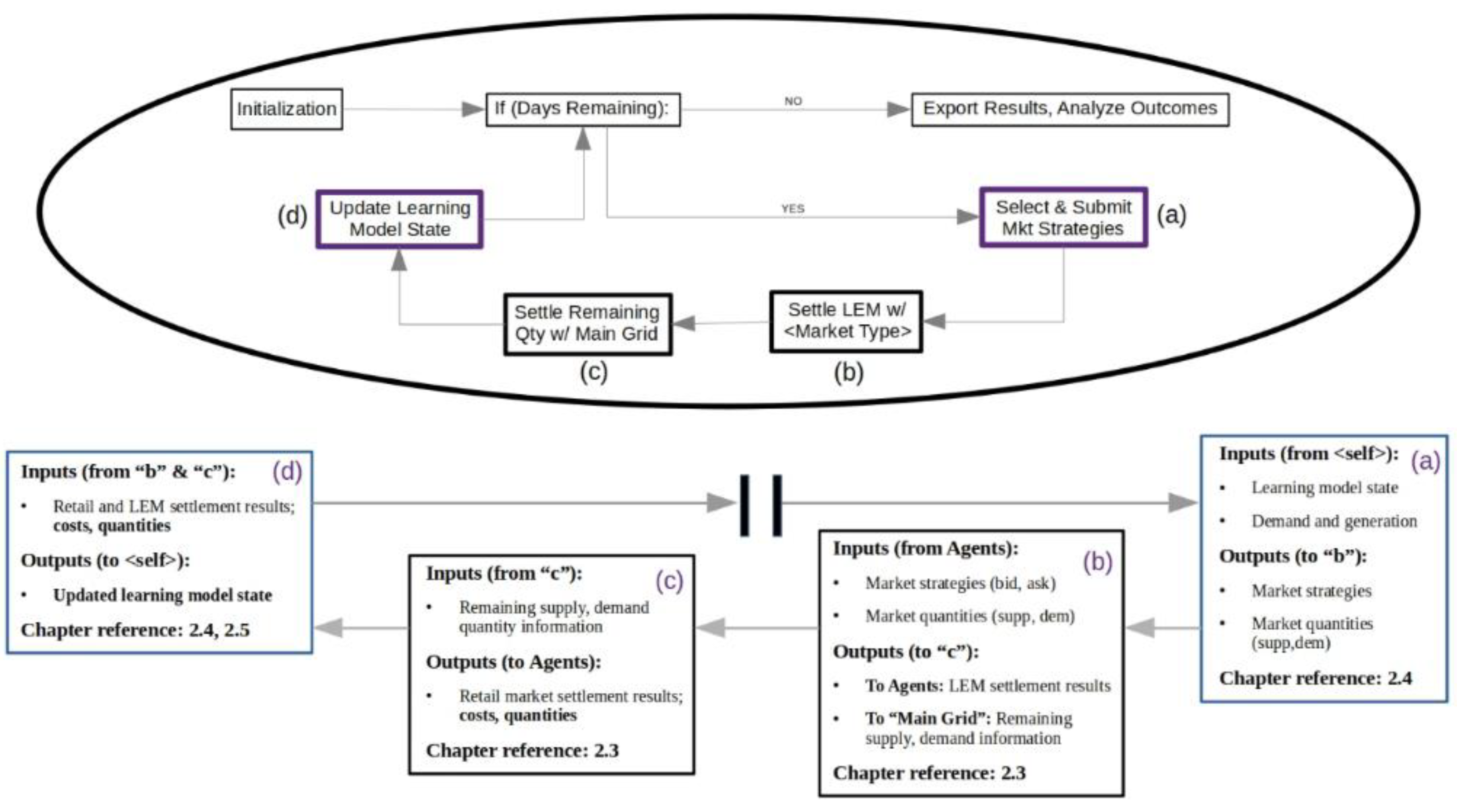
2.1. Simulation Environment Modeling

Household income is modeled as a part of the simulation environment which impacts simulated agents’ initialization conditions. Incorporating an income distribution into agent modeling allows agent behavior to be constrained by economic rationality when market price constraints are lifted. In the current work, household income affects the range of bid prices considered by an agent, and lower-bounds the emphasis placed on own-economic value in utility function calculation. The income distribution described in

Table 2. Overview of agent income distribution modeling, defined using U.S. Census data on annual household income in Kings County, New York, 2019, as presented in [17].

Agent-Level Income Distribution
$$\begin{gathered} \mathbf{Agent} \mathbf{Income} {\mathit{R}}_{\mathit{i}} \\ (\mathbf{in} \mathbf{Thousands} \$\mathbf{USD}) \end{gathered}$$	Population %	Agents Selected (N = 100)
$R_i \in [\$0, \$10]$	8.8	9
$R_i \in (\$10, \$15]$	6.4	6
$R_i \in (\$15, \$14]$	9.6	10
$R_i \in (\$25, \$35]$	8.3	8
$R_i \in (\$35, \$50]$	10.5	11
$R_i \in (\$50, \$75]$	14.1	14
$R_i \in (\$75, \$100]$	11.2	11
$R_i \in (\$100, \$150]$	14.0	14
$R_i \in (\$150, \$200]$	7.4	7
$R_i>\$200$	9.6	10

was observed in Brooklyn, NY, in 2019 [17]. Agents are uniform-randomly selected for each income bracket, and each agent’s income $R_i$ is initialized by a separate uniform random draw between the bracket minimum and maximum incomes. Population proportions in each income bracket are rounded to support simulation implementation. Agents in lowest and highest brackets are assigned the maximum and minimum incomes, $r_{max}$and $r_{min }$respectively.

In the simulated LEM environment, the physical power grid is not modeled—however, a basic model of the power grid owned and operated by Consolidated Edison in the Brooklyn, New York area (NYISO region “J”) provides representation of the retail market corresponding to the local power grid. This retail market is assumed to always be available to all agents, always able to supply consumer demand, and always able to safely accommodate excess prosumer generation. The modeled retail energy price$p_{ret}= \$0.175 \mathrm{usd}/\mathrm{kWh}$represents a typical retail purchase price in Brooklyn, New York, in 2019. Prosumer generation may be purchased by the retail market at the feed-in tariff price$p_{fit}= \$0.053 \mathrm{usd}/\mathrm{kWh}$. This retail market model essentially accounts for agents’ remaining demand or supply after local market settlement, due to its simplicity.

Under the current SDR-based simulation design, all agents are modeled with identical, static values for daily energy demand quantity. Specifically, demand is set to $D_i= 19.64 \mathrm{kW}$ for all agents $i \in I$. To produce specific and distinct supply-demand ratios for market outcome analysis, agents’ daily generation is varied according to the specified SDR for a simulation scenario. Agent behavior in the current work is limited to market price strategy selection; agent behavior with regard to demand response, supply scheduling, etc. are not currently considered in the modeling, due to the current research scope. Agents’ daily energy generation quantity$G_i$is initialized for agents $i \in I$ as shown in Algorithm 1 below. Note that $C_i \in \{0,1\}$is held by each agent to indicate their “type” as consumer ($C_i=1$) or prosumer ($C_i=0$).

Algorithm 1: Daily initialization of agent generation quantities.
1.	For each$i \in I$:
2.	If ($C_i=0$):
3.	$\hspace{1em}\hspace{1em}{G}_i=D_i+\frac{SDR \ast \left( {\sum }_{j\in I_{\mathrm{con}}}{D}_j \right)}{\left|I_{pro}\right|}$
4.	Else: $G_i=0$

Mengelkamp et al. [10] provides one of the most visible LEM design analyses in recent work. Through quantitative evaluation of Brooklyn Microgrid design, the market platform itself is well-described. Based on this previous work, a LEM environment is implemented which is settled using a “uniform double auction” (UDA). In a number of previous works, LEM prices are restricted to the range$p_{loc} \in \left[p_{fit},p_{ret}\right]$; for example, in directly-related works such as [4,11,18,19,20,21]. However, in a number of real-world systems (e.g the Brooklyn Microgrid, which is modeled here) do not appear to make this restriction. Both scenarios are explored by the experiments described in Section 3.1.

The local market is settled according to the uniform-price, double-sided auction settlement described in Algorithm 2. Supply and demand are matched using merit-order supply allocation; prosumers are matched in order of increasing ask price, and consumers are matched with prosumers in order of decreasing bid price. Transaction quantities$Q_{loc,t }$are defined by the minimum of matched agents’ demand and supply quantities. A uniform market-clearing price $p_{loc,t}$is used for all transactions in a given market settlement, which is the bid price of the last-matched consumer in the current LEM settlement. This auction restricts agents’ information to their own market inputs$\{Q_{0,i,t} , S{’}_{i,t}\}$and outputs$\{Q_{loc,i,t} , p_{loc,t}\}$.

Algorithm 2: Overview of modeled double auction, which uses merit-order supply allocation and a uniform, market-clearing price.
1.	For each $t \in T$:
2.	$bidders \leftarrow sort\left(I, current\_bi{d}_{i,t}, > \right)$
3.	$suppliers \leftarrow sort\left(I, current\_as{k}_{j,t}, < \right)$
4.	While ($bidders != \varnothing \wedge suppliers != \varnothing$):
5.	$\hspace{1em} allocate\_supply\left( bidders\left[0\right], suppliers\left[0\right] \right)$
6.	If ($remaining\_deman{d}_{i,t}$ of $bidders\left[0\right] = 0$):
7.	If ($length\left(bidders\right) = 1$):
8.	$\hspace{1em}\hspace{1em}\hspace{1em}\hspace{1em}{P}_{loc,t} \leftarrow current\_bi{d}_{i,t}$ of $bidders\left[0\right]$
9.	Remove $bidders\left[0\right]$ from $bidders$
10.	Else if ($remaining suppl{y}_{i,t}$ of $suppliers\left[0\right] = 0$):
11.	If ($length\left(suppliers\right) = 1$):
12.	$\hspace{1em}\hspace{1em}\hspace{1em}\hspace{1em}{P}_{loc,t} \leftarrow current\_bi{d}_{i,t}$ of $bidders\left[0\right]$
13.	Remove $suppliers\left[0\right]$ from $suppliers$
14.	Calculate and assign transaction costs for time t

2.2. Consumer Agent Modeling

Consumer modeling is largely defined by market utility modeling $V_{i,t}^{con}\left(Q_{i,t},P_{i,t},{\theta }_i\right)$, shown in Equation (1). Consumers’ utility modeling is described in Equations (1)–(3). Equation (1) describes the total utility function, which represents a mutually exclusive balance between a consumer’s own-economic (oe) and “alternative” (alt) sources of value from the LEM settlement.

Consumer value preference parameter ${\theta }_i \in \left[0,1\right]$ indicates the relative measure of emphasis that a consumer agent places on own-economic utility maximization—that is, on energy cost savings. It is a function of local market price and quantity outcomes and is described by Equation (2). When ${\theta }_i=1 \forall i \in I$ and $p_{loc} \in \left[p_{fit},p_{ret}\right]$, consumer utility modeling reflects [11,16]. In the current work, own-economic value is lower-bounded at zero; removing this constraint may support the investigation of research questions related to potentially-irrational user behavior. $Q_{grid,i,t}$ gives retail market purchase quantity for agent i at time t.

In contrast to own-economic utility,$\left(1-{\theta }_i\right)$ represents a consumer’s level of “alternative” utility preference; it represents a user’s “willingness to pay” for LEM-sourced energy supply. Consistent with previous experimental works which evaluate the preferences and motivations of potential LEM users [6,7,9,22], this “alternative” value preference represents the value that a consumer derives from local energy purchase due to environmental, socio-economic, or other motivations. Under the assumption that LEM energy is fully carbon-neutral, and sourced directly from local households with ecologically sustainable siting for RERs, LEM energy purchases are well-aligned with these value preferences.

$$V_{i,t}^{con}\left(Q_{i,t},P_{i,t},{\theta }_i\right)=\left({\theta }_i \ast u_{oe,i,t}\right)+{\displaystyle (}(1-{\theta }_i)\ast u_{alt,i,t}{\displaystyle )}$$

(1)

$$u_{oe,i,t}={\theta }_i \ast min\left[ 0, \left(\left(p_{ret,i,t} \ast Q_{grid,i,t}\right)-\left(P_{loc,i,t} \ast Q_{loc,i,t}\right)\right) \right]$$

(2)

$$u_{alt,i,t}=\left(1-{\theta }_i\right) \ast \left(max\left[s \in S_i\right] \ast Q_{loc,i,t}\right)$$

(3)

Market strategies $s \in S_i$ considered by each consumer represent prices that (1) the agent is rationally able and willing to pay on behalf of the LEM user household, and (2) are allowed by the LEM platform. The initialization of bid range $S_i$ is specific to individual agents and is described in Section 2.4. Here, a rational interpretation of bid range supports modeling of “alternative” utility.

Equation (3) describes “alternative” (alt) utility as a user’s private “reserve price” for energy$s_{max,i}=max\left[s \in S_i\right]$. This price captures all value sources for the agent, including “alternative” value preference; it may also be referred to as the agent’s “reserve price”, or true valuation of local energy. We note that the current formulation does not yet clearly distinguish between the influences of individual preferences (or own-economic preference specifically) on$s_{max,i}$, but also note (from Section 1) that “alternative” value factors generally represent the majority of influential value sources noted by potential LEM users in cited studies.

2.3. Prosumer Agent Modeling

Prosumer utility $V_{i,t}^{pro}\left(Q_{i,t},P_{i,t},{\theta }_i\right)$ is described by Equation (4) as the sum of utility derived from sales to the retail grid market, and from the local market. In Equation (5), prosumers’ valuation of retail grid profits is modeled identically for all agents, as in previous work [11,16]. Local sale valuation, however, depends on prosumer value preference parameter${\theta }_i \in \{1,2,3\}$. Prosumers’ ${\theta }_i$ indicates a specific preference “type”, which determines their sensitivity to changes in local market price; the specific form of Equation (6) used by a given prosumer to determine local market settlement utility is determined by ${\theta }_i$. For preference type ${\theta }_i=1$, local sales profits describe expected prosumer utility in Equation (6), reflecting prosumer utility modeling presented in [11,21] and utilized in [16]. Consistent with previous work, RER operation costs are approximated to zero, reflecting the low marginal cost of PV panel operation.

Prosumers have been noted in a number of recent works to hold a wide range of motivations for RER uptake and value preferences for LEM sales [6,8,9,23,24]. Consistent among these works is the identification of own-economic value maximization as a motivating factor. However, value preferences are noted which do not necessarily depend on sale price—examples include a prosumer’s derived value from supporting carbon emissions reduction, realizing energy autarky, or supporting their local community. The maximum-allowed prosumer asking price ($p_{ret}$) represents an upper-limit to the per-unit sales value that a prosumer can expect from the LEM. Due to the price-inelastic nature of “alternative” value sources, prosumers with preference type ${\theta }_i=3 \mathrm{a}$re modeled as retaining value from market settlement independent of local price fluctuations.

$$V_{i,t}^{pro}\left(Q_{i,t},P_{i,t},{\theta }_i\right)=grid\_va{l}_{i,t}+local\_va{l}_{i,t}$$

(4)

$$grid\_va{l}_{i,t}=Q_{ret,i,t} \ast p_{fit}$$

(5)

$$local\_va{l}_{i,t}=y$$

(6)

where if (${\theta }_i=1$):

$$y=Q_{loc,i,t} \ast P_{loc,i,t}$$

else if (${\theta }_i=2$):

$$low=p_{ret}-\left(\left(p_{ret}-p_{fit}\right) \ast \left(1-0.3714\right)\right)$$

$$pct=\left(P_{loc,i,t}-p_{fit}\right) / \left(p_{ret}-p_{fit}\right)$$

$$y={\displaystyle (}\left(low+\left(\left(p_{ret} \ast low\right) \ast pct\right)\right) Q_{loc,i,t}{\displaystyle )}$$

else:

$$y=Q_{loc,i,t} \ast p_{ret}$$

Prosumer utility for preference “type” ${\theta }_i=2 \mathrm{r}$epresents a prosumer with “mixed” value preference; in other words, a prosumer which may simultaneously hold both own-economic and “alternative” valuations for energy sales. The value function in Equation (6) for Type-2 prosumers is modeled based on sale preference data described in [24] for prosumer cluster B. Since energy storage is not represented in the current work, the average decrease in sale probability between maximum and minimum market prices (across all battery charge states presented in the cited experiment) is compared to that of prosumer cluster A, to describe the difference in relative utility decrease (as indicated by sale probabilities) for cluster B prosumers compared to cluster A prosumers. The relative utility decrease for cluster B prosumers is ~37% less, on average, than for cluster A; this relatively reduced “elasticity” in sale utility is described by$V_{i,t}^{pro}(Q_{i,t},P_{i,t},{\theta }_i=2)$.

2.4. Agent-Level Parameter Initialization

The current study is interested in evaluating socio-economic impacts of LEM outcomes which are generated by (1) input factors shaped by “external” socio-economic conditions, and (2) market dynamics produced by a given mechanism design. As an initial step, agent parameters and decision-making are shaped by random functions of household income $R_i$, individual value preference ${\theta }_i$, and the feedback loop between an agent’s selected market strategies and their market settlement outcomes. Agent-level parameter initialization is shown in Algorithm 3.

After agents’ incomes $R_i$ are assigned as in Section 2.1, preference parameters ${\theta }_i$ are set for each agent, and the bounds of each agent’s considered market strategy range are set. As noted previously, consumer ${\theta }_i \in \left[0,1\right]$ indicates emphasis on own-economic value, while prosumer ${\theta }_i \in \{1,2,3\}$indicates preference type, between “own-economic” (${\theta }_i=1$), “alternative” (${\theta }_i=3$), and “mixed” (${\theta }_i=2$). For consumers and prosumers both, $s_{max,i}$ constrains agents’ range of potential market strategies $S_{i,t}$.

Prosumer preference type ${\theta }_i$ is set on Line 15 using a multinomial distribution on a set of relative probabilities $\Pi = \{ {\pi }_1, {\pi }_2, {\pi }_3 \}$ of assigning a given type value. The relative probabilities in $\Pi$ are held constant in a given simulation but may be defined differently between simulations. As a localized distribution has not yet been defined, a range of distributions are tested in Experiment 2 (Section 3.1).

Prosumers’ maximum asking price$s_{max,i}$ is to $p_{ret}$ on Line 14 (Algorithm 3). However, the range of bidding prices considered by each consumer agent is set between $p_{fit}$ and an individualized upper bid limit $s_{max,i}$ (set on Line 6). This is the maximum bid price that a consumer will consider selecting as a market strategy; it is based on willingness to pay, and ability to pay. “Ability to pay” is represented by ${\delta }_i$ on Line 8. Variable ${\delta }_i$ determines if (and by how much) the consumer is rationally able to bid higher than the retail price. A consumer agent’s willingness to pay above $p_{ret}$ in the local market, then, is given by ${\delta }_i \ast \left(1-{\theta }_i\right)$ in Line 6.

Algorithm 3: Initialization of agent types and behavioral parameters
1.	Randomly select $|I_{con}| = 75$ agents (no replacement):
2.	Set $C_i = true$// initialize consumer
3.	Set $R_i$ as in Section 2.1
4.	Set ${\theta }_i \sim Uniform\left( \left(1 - \frac{R_i - r_{min}}{r_{max} - r_{min}}\right), 1 \right)$
5.	Set $P_i^{*} = \left[ \left(R_i / T\right) \ast e’ \right] / EST$
6.	Set $s_{max,i} = p_{ret} + \left(\delta \ast \left(1 - {\theta }_i\right) \right)$
7.	where:
8.	$\hspace{1em}\hspace{1em}{\delta }_i=max\left[ 0, \left(P_{max,i}-p_{ret}\right) \right]$
9.	$\hspace{1em}\hspace{1em}{P}_{max,i}=\left[ \left(R_i / T\right) \ast upper\_\underset{}{\lim } \right] / D_i$
10	$\hspace{1em}\hspace{1em}{\mathrm{upper}\_\lim }_i=e_{obs} \ast \left(1-\frac{R_i-r_{min}}{r_{max}-r_{min}}\right)$
11.	Randomly select $|I_{pro}| = 25$ agents (no replacement):
12.	Set $C_i = false$// initialize prosumer
13.	Set $R_i$as in Section 2.1
14.	Set$s_{max,i} = p_{ret}$
15.	Set${\theta }_i \sim Multinomial\left( 1, \Pi \right)$
16.	where:
17.	$\hspace{1em}\hspace{1em}\Pi = \{ {\pi }_1, {\pi }_2, {\pi }_3 \}$such that:
18.	$\hspace{1em}\hspace{1em}\hspace{1em}{\pi }_{j \in \{1,2,3\}}=Prob \left({\theta }_i=j\right)$
19.	and $\left({\sum }_{\mathrm{j}\in \left\{1,2,3\right\}}{\pi }_j\right)=1$
20.	For all agents $i \in I$:
21.	Set $S_{i,t} = \{ p_{fit}, \dots , s_{max,i} \}$

Rationality in considered bid price (${\mathrm{upper}\_\lim }_i$, Line 10) scales inversely with income, from a conservative estimate $e_{obs}=13\%$ of local low-income energy cost burden, as a percentage of household income. Consistent with static, uniform energy demand $D_i \forall i \in I$, the variable ${\mathrm{upper}\_\lim }_i$ constrains all agents’ maximum energy costs to be at or below an upper-end observed cost for real-world energy consumers locally ($e_{obs} \ast p_{ret}$), noting that this cost constitutes an increasingly-small proportion of household income $R_i$, as income increases from $r_{min}$ to $r_{max}$.

Consumer price target $P_i^{\ast }$ is described (on Line 5) as an energy purchase price which makes an equitable supply threshold (EST) quantity of energy affordable to agent i with just $e\prime =6\%$ of household income$R_i$. Consistent with [25,26,27], we consider an EST quantity of energy consumption to allow for a full, equitable level of participation in modern life locally. Specific EST quantities may vary spatially and temporally, and may be defined differently across demographic groups in a local area. In the current study, $EST=\mu \left[ D_{i \in I} \right]$, denoting the unweighted mean individual energy demand across all agents.

2.5. Agent Learning & Behavior

In the current work, user-agent behavior is limited to price strategy selection, in order to isolate the combined impacts of user value preferences $\theta$ on market settlement. As noted previously, “strategies” in the current work refer to consumers’ bidding prices and prosumers’ asking prices, for energy offered by local prosumers in the LEM. Agents behave according to the Modified Roth-Erev (MRE) reinforcement learning algorithm presented in [21], which describes a stochastic approach to individual utility maximization. The MRE algorithm has more recently been demonstrated in [11] and self to support simulation-based LEM mechanism design evaluation, consistent with the original empirical context of learning algorithm development [28].

The MRE algorithm takes two parameters $\lambda$ and $ϵ$, representing learning rate and memory, respectively. Consistent with [16], parameter values of $\lambda =0.083$ and $ϵ=0.01 \mathrm{a}$re set for all agents, to support efficient and rational behavior which may, theoretically, be taken to represent expected user behavior in the modeled LEM setting. The learning parameters mediate the influence of the agent’s utility perception on the update of strategy propensities $u_{i,s,t+1}$ in Equation (7), for each considered strategy $s \in S_i$ of a given agent i. Strategy propensities are used in Equation (8) to derive the relative probability $x_{i,s,t+1}$ of each considered strategy $s \in S_i$; Equation (9) then collects relative probabilities$x_{i,s,t+1}$into the set$X_{i,t+1}$, used in strategy selection. Overall, the MRE algorithm takes individual market settlement results$\{Q_{i,t},P_{i,t}\}$at each time step and produces a market strategy selection$S_{i,t+1}^{\prime }$as a function of individual utility, according to Algorithm 4.

$$u_{i,s,t+1}=\left(1-\lambda \right)\ast u_{i,s,t}+\left\{\begin{array}{c}{V}_{i,t}\left(Q_{i,t},P_{i,t},{\theta }_i\right)\ast \left(1-ϵ\right) (\mathrm{if} s=S_{i,t}^{\prime })\\ \hspace{0.17em}\hspace{0.17em}\hspace{0.17em}\hspace{0.17em}\hspace{0.17em}\hspace{0.17em}\hspace{0.17em}\hspace{0.17em}\hspace{0.17em}\hspace{0.17em}\hspace{0.17em}{u}_{i,s,t} \ast \left(\frac{ϵ}{\left|S_i\right|-1}\right) \left(\mathrm{otherwise}\right)\end{array}\right.$$

(7)

$$x_{i,s,t+1}=\frac{u_{i,s,t+1}}{\left(\sum u_{i,s,t+1}\right)}$$

(8)

$$X_{i,t+1}= \{x_{i,1,t+1}, x_{i,2,t+1}, \dots ,x_{i,\left|S_i\right|,t+1}\}$$

(9)

At the agent level, simulations follow the execution loop described by Algorithm 4, which implements the MRE algorithm. Agents choose strategies at random from a $Multinomial\left(\left|S_i\right|,X_{i,t}\right)$ distribution, where the vector $X_{i,t}$ contains the relative probabilities of each strategy in an agent’s considered strategy set $S_i$. When market settlement results $\{ Q_t, P_t \}$ are received by agents, updated strategy probabilities $X_{i,t+1}$ are calculated for the following time-step according to market results, preference parameter ${\theta }_i$, and utility function $V_{i,t}^{con}$ or $V_{i,t}^{pro}$ (Equations (1) and (4), respectively), depending on agent type $C_i$, which is set using Algorithm 3.

Algorithm 4: Overview of Modified Roth-Erev learning algorithm for double-sided auction behavior representation in energy market.
1.	For market settlements $t \in T$:
2.	For agents $i \in I$:
3.	Draw $S{’}_{i,t} \sim Multinomial\left( |S_i|, X_{i,t} \right)$
4.	Submit strategy $S{’}_{i,t}$ to LEM
5.	Receive LEM settlement results:$\{ Q_t, P_t \}$
6.	Calculate $X_{i,t+1}$ via Equations (7)–(9), such that:
7.	If ($C_i > 0$): // if agent is “consumer” type
8.	$\hspace{1em}\hspace{1em}\hspace{1em}\hspace{1em}{V}_{i,t}\left(Q_{i,t},P_{i,t},{\theta }_i\right)\leftarrow V_{i,t}^{con}\left(Q_{i,t},P_{i,t},{\theta }_i\right)$
9.	Else: // if agent is “prosumer” type
10.	$\hspace{1em}\hspace{1em}\hspace{1em}\hspace{1em}{V}_{i,t}\left(Q_{i,t},P_{i,t},{\theta }_i\right)\leftarrow V_{i,t}^{pro}\left(Q_{i,t},P_{i,t},{\theta }_i\right)$

2.6. Results Analysis Metrics

Standard techno-economic requirements for mechanism design include individual rationality, incentive compatibility, technical market efficiency, stability of outcomes, and supply-demand pricing (that is, local market supply increase is not expected to produce local price increase) [29]. First-price auctions, including UDA-based mechanisms, do not produce truthful bidding relative to true valuations, as a dominant strategy. They have been shown to converge rapidly to one of potentially many Nash equilibria, and may potentially converge to a cycle between a set of equilibrium points (illustrated in [16]). Here, techno-economic metrics are taken as validation and analysis metrics, but the focus of analysis is placed on socio-economic outcomes which have been noted to impact the participation intentions of potential LEM users: energy affordability and market access. Along with being relevant to potential LEM users, market access and affordability outcomes have been identified empirically as key shortcomings in current retail markets [30]. Both sets of metrics are presented together in Table 3.

Table 3. Socio-economic metrics for analysis of LEM mechanism simulation results.

Results Analysis Metrics (Per Simulation)
Metric Name	Metric Calculation
Agent Rationality Measurement	$AR{M}_t=\frac{{\sum }_{i\in I}Ind\left[ V_{i,t}\left(Q_{i,t},P_{i,t},{\theta }_i\right) \ge 0 \right]}{\left|I\right|}$	(10)
Technical Market Efficiency	$\mathrm{If} (SD{R}_t>1$):
	$TM{E}_t=\left({\sum }_{i\in I_{\mathit{con}}}{Q}_{loc,i,t}\right) / \left({\sum }_{i\in I_{\mathit{con}}}{Q}_{0,i,t}\right)$	(11)
	Else:
	$TM{E}_t=\left({\sum }_{j\in I_{\mathit{pro}}}{Q}_{loc,j,t}\right) / \left({\sum }_{j\in I_{\mathit{pro}}}{Q}_{0,j,t}\right)$	(12)
Consumer Relative Market Access	$RMA{c}_{i,t}=\frac{min\left[ 1, \left(Q_{loc,i,t} / EST\right) \right]}{min\left[ 1, \left(max\left[ Q_{loc,con,t} \right] / EST\right) \right]}$	(13)
Prosumer Relative Market Access	$RMA{p}_{i,t}=\frac{Q_{loc,i} / \left({\sum }_{j\in I}{Q}_{loc,j}\right)}{max\left[ Q_{loc,pro }/ \left({\sum }_{j\in I}{Q}_{loc,j}\right) \right]}$	(14)
Consumer Energy Cost Burden	$\mathrm{If} Q_{loc,i,t}<EST$:
	$EC{B}_{i,t}=\frac{\left(P_{loc,i,t} \ast Q_{loc,i,t}\right)+\left(\left(EST-Q_{loc,i,t}\right) \ast p_{ret}\right)}{EST} / P_i^{*}$	(15)
	Else:
	$EC{B}_{i,t}=\frac{P_{loc,i,t}}{P_i^{\ast }}$	(16)
Mean Market Price	$MMP=\frac{{\sum }_{t\in T}\left[ \left({\sum }_{i\in I}{P}_{loc,i,t}\right)/|I| \right]}{\left|T\right|}$	(17)

Table 3. Socio-economic metrics for analysis of LEM mechanism simulation results.

Results Analysis Metrics (Per Simulation)
Metric Name	Metric Calculation
Agent Rationality Measurement	$AR{M}_t=\frac{{\sum }_{i\in I}Ind\left[ V_{i,t}\left(Q_{i,t},P_{i,t},{\theta }_i\right) \ge 0 \right]}{\left|I\right|}$	(10)
Technical Market Efficiency	$\mathrm{If} (SD{R}_t>1$):
	$TM{E}_t=\left({\sum }_{i\in I_{\mathit{con}}}{Q}_{loc,i,t}\right) / \left({\sum }_{i\in I_{\mathit{con}}}{Q}_{0,i,t}\right)$	(11)
	Else:
	$TM{E}_t=\left({\sum }_{j\in I_{\mathit{pro}}}{Q}_{loc,j,t}\right) / \left({\sum }_{j\in I_{\mathit{pro}}}{Q}_{0,j,t}\right)$	(12)
Consumer Relative Market Access	$RMA{c}_{i,t}=\frac{min\left[ 1, \left(Q_{loc,i,t} / EST\right) \right]}{min\left[ 1, \left(max\left[ Q_{loc,con,t} \right] / EST\right) \right]}$	(13)
Prosumer Relative Market Access	$RMA{p}_{i,t}=\frac{Q_{loc,i} / \left({\sum }_{j\in I}{Q}_{loc,j}\right)}{max\left[ Q_{loc,pro }/ \left({\sum }_{j\in I}{Q}_{loc,j}\right) \right]}$	(14)
Consumer Energy Cost Burden	$\mathrm{If} Q_{loc,i,t}<EST$:
	$EC{B}_{i,t}=\frac{\left(P_{loc,i,t} \ast Q_{loc,i,t}\right)+\left(\left(EST-Q_{loc,i,t}\right) \ast p_{ret}\right)}{EST} / P_i^{*}$	(15)
	Else:
	$EC{B}_{i,t}=\frac{P_{loc,i,t}}{P_i^{\ast }}$	(16)
Mean Market Price	$MMP=\frac{{\sum }_{t\in T}\left[ \left({\sum }_{i\in I}{P}_{loc,i,t}\right)/|I| \right]}{\left|T\right|}$	(17)

Market efficiency and individually rational participation are theoretically expected properties of the UDA mechanism [3,9,13,18,20,21,29]. In the current results, these metrics are presented numerically as means of further validating simulation implementation. Individual rationality is measured in Equation (10) as the percentage of agents with non-negative utility from LEM participation. Note that the function $Ind\left[x\right]$ evaluates some input x as a Boolean expression; when $x=true$, $Ind\left[x\right]=1$; when $x=false$,$Ind\left[x\right]=0$. Technical market efficiency is measured by Equations (11) or (12), depending on the local-level supply-demand ratio. When supply is less than demand (i.e.,$SDR<1$), a technically efficient market allocates all supply locally; when supply at least equals demand (i.e.,$SDR \ge 1$), all local demand should be satisfied by local supply.

Grid level technical performance metrics may be integrated as well; for example, [19,20] use a “power flatness index” for assessing the level of temporal matching between the aggregate of agents’ market supply and demand profiles. Power flatness is a desirable goal which may support transmission grid stability e.g., in terms of line voltage and local self-sufficiency. As the current work utilizes an SDR-based simulation approach, power flatness is described by a combination of technical market efficiency ($TME$) and the supply-demand ratio itself; power flatness is maximized when $TME=1$ and $SDR=1$. Based on Section 4.2, power flatness may be approximately satisfied by IP agents (or platform users, modeled by IP agents) under LEM operation in a target SDR range where SDR is close to 1.

While technical market access is provided for all LEM users, the actual sale or purchase quantities seen by individual agents may be highly varied depending on mechanism design characteristics. In previous work [16], “identical” agents experienced a range of outcomes under the UDA mechanism, in an otherwise-similar simulation environment to this present work. Consumers’ Relative Market Access metric ($RMAc$) aims to more fully represent “access equality” in the current work, rather than “outcome equality” as measured by the Equality Index presented in [19,20]. Energy equity objectives are taken as theoretical grounding for socio-economic metrics, consistent with [25,26,27]. In energy distribution, equity does not necessarily require uniform market outcomes, but a uniform ability of all agents to secure comparable energy demands may be expected from LEM settlements. To check satisfaction of this requirement, $RMAc$ compares the proportion of EST satisfied by the current market settlement, to the highest satisfaction proportion observed across all consumers in that settlement. In this way, a relative measure of market access is described; $RMA{c}_{i,t}=1 \mathrm{i}$mplies that agents are able to obtain similar percentages of their EST quantity satisfied locally. $RMA{c}_{i,t}=0.5$ indicates that agent i has secured a 50% lower proportion of EST, relative to the highest proportion satisfied at time t.

Supply units are effectively interchangeable from a consumer’s perspective, under assumption of uniform quality. Scenarios in which transmission costs are passed on to consumers, or which may produce unique prices in each transaction (e.g., double auction with discriminatory pricing), may require an updated formulation. With no distinguishing factor in a given unit of supply, it is unclear how differentiated market access claims would be made by prosumers; this suggests that a goal of equal market access may also be applied to prosumers. A goal of equal prosumer market access also has the desirable property of measuring whether or not a new local prosumer in the LEM may reasonably expect to find value in participation, under a given set of pre-existing market supply conditions. For prosumers’ Relative Market Access ($RMAp$), each prosumer’s sale quantity is compared in Equation (14) to the maximum-observed sale quantity at a given settlement time, in order to evaluate consistency in market share across prosumers.

The Energy Cost Burden metric ($ECB$) calculates consumers’ energy “affordability gap”, defined as the percent difference between the household’s realized energy costs, and the cost of securing an EST quantity of energy at an individually affordable price. We claim that this interpretation is consistent with current approaches to energy affordability calculation [1,15,31,32]. The use of Equations (15) or (16) to calculate$EC{B}_{i,t}$depends on$Q_{loc,i,t}$. If agent i was not able to secure an EST quantity locally, additional retail market costs are considered in Equation (15); otherwise, Equation (16) is used, which simply compares realized energy price$P_{loc,i,t}$ to an individually affordable energy price $P_i^{\ast }$. For example, at$EC{B}_{i,t}=1$, an agent’s energy cost is precisely at the 6% affordability threshold $e\prime$; when$EC{B}_{i,t}=2$, energy costs require$2 \ast e\prime =12\%$of household income.

In the current work, Mean Market Price (MMP) is used to evaluate LEM price expectations. The mean LEM price in a simulation run is calculated according to the MMP metric (Equation (17)). As it is a simulation-level metric, a subscript is not used. The mean LEM price is taken for each simulation step (which is trivial when$P_{loc,t}$is a uniform price), and then the mean price across all $t \in T$is calculated.

3. Experiments

In the current study, expected LEM outcomes are analyzed under the simulated uniform double auction (UDA) mechanism described in Section 2.1, using the evaluation metrics presented in Section 2.6. In six tests, local-level SDR is taken as a variable parameter; agents’ demand D is held constant at an estimated 2019 daily average for a household in Brooklyn, New York City [33], while prosumer generation G is varied by SDR. For each SDR within a simulation test, 100 simulation runs (with 365 observations each) are recorded. In each simulation, 100 agents are randomly assigned to be “consumer” or “prosumer” type; 75 consumers and 25 prosumers are chosen at random as in Algorithm 3, approximating the type-proportion reported in a trial of the Brooklyn Microgrid platform [34]. Results metrics are calculated from each simulation run, collected, and grouped by SDR, for each parameter combination considered in each test. Step-wise results metrics (i.e., all metrics except for MMP) are averaged across T simulation steps; mean values are computed for each metric, across all runs, for each SDR in a given test. Market price convergence is observed within 60 simulation steps in preliminary testing, using the parameter tuning in Section 2.5; based on this observation, all simulations run for 90 steps before results data were collected for analysis.

Simulated agents in the current work are referred to as “IP agents”, for the income-preference heterogeneous agents described in Section 2.2, Section 2.3 and Section 2.4. This is in contrast to the “identical” agents modeled in previous works [11,16]. Agents in these previous works are identically modeled and initialized, holding${\theta }_i=1$ and $S_i= \{p_{fit},\dots ,p_{ret}\}$across all agents.

3.1. Experiment Parameters

Table 4. Summary of variable parameters included in each simulation experiment.

Simulation Parameters by Experiment
		Experiment 0	Experiment 1	Experiment 2
Test Number(s)		1	{2, 3, 4, 5}	6
Parameters	$\Pi$	(0.33, 0.33, 0.33)	(0.33, 0.33, 0.33), (0.5, 0.25, 0.25), (0.25, 0.5, 0.25), (0.25, 0.25, 0.5)	(0.33, 0.33, 0.33)
	K	True	True	False
	SDR	{0.01, 0.1, 0.2, …, 2.0}	{0.01, 0.1, 0.2, …, 2.0}	{0.01, 0.1, 0.2, …, 2.0}
	M	“Baseline”	“UDA”	“UDA”

provides a summary of parameters used in the current study. Consistent with [16], generalizing LEM analysis results to improve analysis robustness, and avoid un-controlled influence of system-specific operation conditions on mechanism analysis, is emphasized. To this end, an SDR-based simulation approach is again used. To describe a “baseline” for results analysis, Test 1 (Experiment 0) simulates the retail energy market mechanism in Section 2.1. The parameter M notes the mechanism used in corresponding market settlements.

$\Pi$A local type distribution for prosumer value preferences has not been specified for the simulated Brooklyn Microgrid area, and while a growing number of works have presented data on prosumers’ LEM value preferences and participation motivations, we do not assume that these factors will be similar across spatio-temporal or socio-economic circumstances. Experiment 1 considers a sensitivity analysis on $\Pi$, the distribution of prosumer preference “types” described in Section 2.3. In Test 2, prosumer preference types are drawn from a multinomial probability distribution ${\theta }_{pro} \sim Multinom (n=3, \Pi =\{0.33,0.33,0.33\left\}\right)$ which gives each possible preference “type” ${\theta }_i \in \{1,2,3\}$ an equal probability of being applied to a prosumer. Prosumer type distribution $\Pi =\{0.5,0.25,0.25\}$ is used in Test 3. $\Pi =\{0.25,0.5,0.25\}$ and $\Pi =\{0.25,0.25,0.5\}$ for Tests 4 and 5.

A number of previous works (e.g., [4,11,18,21]) assume that the bids of LEM users (or their software agents) are restricted to the range $p_{loc} \in \left[p_{fit},p_{ret}\right]$. However, real-world LEMs do not necessarily make this assumption; the Brooklyn Microgrid, for example, does not appear to [10]. In Experiment 2, Test 6 holds$K=false$, indicating that all agents’ hold$S_i= \{p_{fit}, \dots , p_{ret}\}$. In Experiment 2, Test 6,$\Pi =\{ 0.33,0.33,0.33\}$is held to simplify comparison with Experiment 1.

As in previous work [16], market outcomes under a range of local-level supply-demand ratios (SDRs) are evaluated for each simulation test indicated. To support clear and concise results discussion, SDRs are grouped together in the analysis. “Low-SDR” describes simulations in which$SDR \in \{0.01,0.2,0.4,0.6\}$. “Target-SDR” simulations are represented by$SDR \in \{0.8,1.0,1.2\}$; local-level supply is approximately equal to demand, indicating a target operation state for LEMs and their underlying power systems. In “High-SDR” conditions, represented here by$SDR \in \{1.4,1.6,1.8,2.0\}$, supply may be notably greater than demand. High SDRs may produce desirable market conditions for consumers, but over time they may also present voltage stability issues for the underlying power system. In future work, these cut-offs may be tuned to reflect goals and constraints for specific real-world systems, and may be correlated with specific stability thresholds.

3.2. Simulated Agent Results Clustering

Consistent with [25], group-level analysis is taken to be fundamental to the assessment of socio-economic impacts from LEM operation. In the current work, agent-level outcomes are computed at the individual level, and are aggregated according to the agent clusters described in Table 5. Consumer agent heterogeneity is captured in two main parameters, income ($R_{con}$) and value preferences (${\theta }_{con}$); prosumer agent heterogeneity is captured by prosumer “types” (${\theta }_{pro}$). The agent clustering in Table 2 is defined to support dis-aggregated analysis of heterogeneity impacts, even while agent results are aggregated into cluster groupings.

Table 5. Overview of agent outcome clustering. Labels are given to provide concise reference in Section 4 results figures.

Results Clustering by Agent Type
$\mathbf{Consumers}: i \in I_{con}$		$\mathbf{Agent} \mathbf{Income} {\mathit{R}}_{\mathit{i}} \in [\mathbf{10}, \mathbf{200}] (\mathbf{in} \mathbf{Thousands} \$\mathbf{USD})$
		Low-Income: $R_i \in (10,35]$	Middle-Income: $R_i \in (35,95.5]$	High-Income: $R_i \in (95.5,200]$
Value Preference: ${\theta }_i\in [0,1]$	${\theta }_i \in [0.9,1]$	Con 1	Con 2	Con 4
	${\theta }_i \in [0.64,0.9)$		Con 3	Con 5
	${\theta }_i \in (0,0.64)$			Con 6
$\mathbf{Prosumers}: i \in I_{pro}$
Value Preference: ${\theta }_i\in \{1,2,3\}$	${\theta }_i=1$	Pro 1
	${\theta }_i=2$	Pro 2
	${\theta }_i=3$	Pro 3

Table 5. Overview of agent outcome clustering. Labels are given to provide concise reference in Section 4 results figures.

Results Clustering by Agent Type
$\mathbf{Consumers}: i \in I_{con}$		$\mathbf{Agent} \mathbf{Income} {\mathit{R}}_{\mathit{i}} \in [\mathbf{10}, \mathbf{200}] (\mathbf{in} \mathbf{Thousands} \$\mathbf{USD})$
		Low-Income: $R_i \in (10,35]$	Middle-Income: $R_i \in (35,95.5]$	High-Income: $R_i \in (95.5,200]$
Value Preference: ${\theta }_i\in [0,1]$	${\theta }_i \in [0.9,1]$	Con 1	Con 2	Con 4
	${\theta }_i \in [0.64,0.9)$		Con 3	Con 5
	${\theta }_i \in (0,0.64)$			Con 6
$\mathbf{Prosumers}: i \in I_{pro}$
Value Preference: ${\theta }_i\in \{1,2,3\}$	${\theta }_i=1$	Pro 1
	${\theta }_i=2$	Pro 2
	${\theta }_i=3$	Pro 3

The three modeled prosumer preference types ${\theta }_i \in \{1,2,3\}$define prosumer clusters Pro 1–Pro 3. For consumers, clustering produces six income/preference parameter combinations. A comparison between Con 1 and Con 4, for example, may help describe outcome differences attributable to income heterogeneity, holding value preference effectively constant. Conversely, comparing Con 4 and Con 6 may help describe outcome differences attributable to value preference differences among users within the same income range. Three potential combinations of consumer clustering parameters are excluded, due to current rationality constraints on consumers’ expression of ${\theta }_i$.

Each cluster contains approximately 1/3 of all same-type agents, ensuring sample size consistency. The range of ${\theta }_i$ for each consumer group is lower bounded by the minimum ${\theta }_i$ modeled for the corresponding income groups. Low-income consumers are at or below the 2019 poverty threshold of $35,000/per year (for a mean household size) in Brooklyn, New York [35], and middle-income median is approximately the 2019 median household income for Brooklyn, New York [17]. “High income” represents the upper 1/3 of the modeled income range.

4. Results & Discussion

The presented work extends on current modeling and evaluation methodologies for LEM mechanism design analysis. Study conclusions are relevant to LEM design in the Brooklyn Microgrid context, but are also applicable to any real-world LEM with similar local income distribution, distribution of local-level supply and demand (among prosumers and consumers respectively), and pricing conditions in a pre-existing retail market. An additional data analysis step is required to apply the presented study results to a specific LEM operation setting, but the generalized analysis approach used here ensures that the accuracy of outcome expectations can be maintained even as power grid conditions change.

For example, previous studies commonly use specific power load time-series data to produce expected LEM outcomes; as the impacts of climate change increasingly affect energy consumption and generation profiles, the results of these studies may become increasingly inaccurate. Current study results can be expected to be more robust, allowing for maintained accuracy under varying local conditions, e.g., climatic conditions, as long as local retail market and socio-economic conditions remain similar to the simulation modeling described here. As differences in these conditions grow, or as supply or demand vary from the mean values assumed in this study, updated outcome analysis is increasingly suggested. While they remain similar to currently-considered conditions, however, results may apply to a range of system implementations and deployment scenarios.

On results figures for RMA (including RMAc and RMAp) and ECB, note that line color brightness indicates SDR scenario: low, target, or high SDR corresponds to light, medium, or dark color respectively. This distinction is also indicated on the appropriate plot legends. In the rest of the current section, the impact of IP agents (defined in Section 3; describes agents modeling presented in Section 2) on LEM outcome expectations is evaluated according to the results metrics presented in Section 2.6, to address the research question from Section 1.

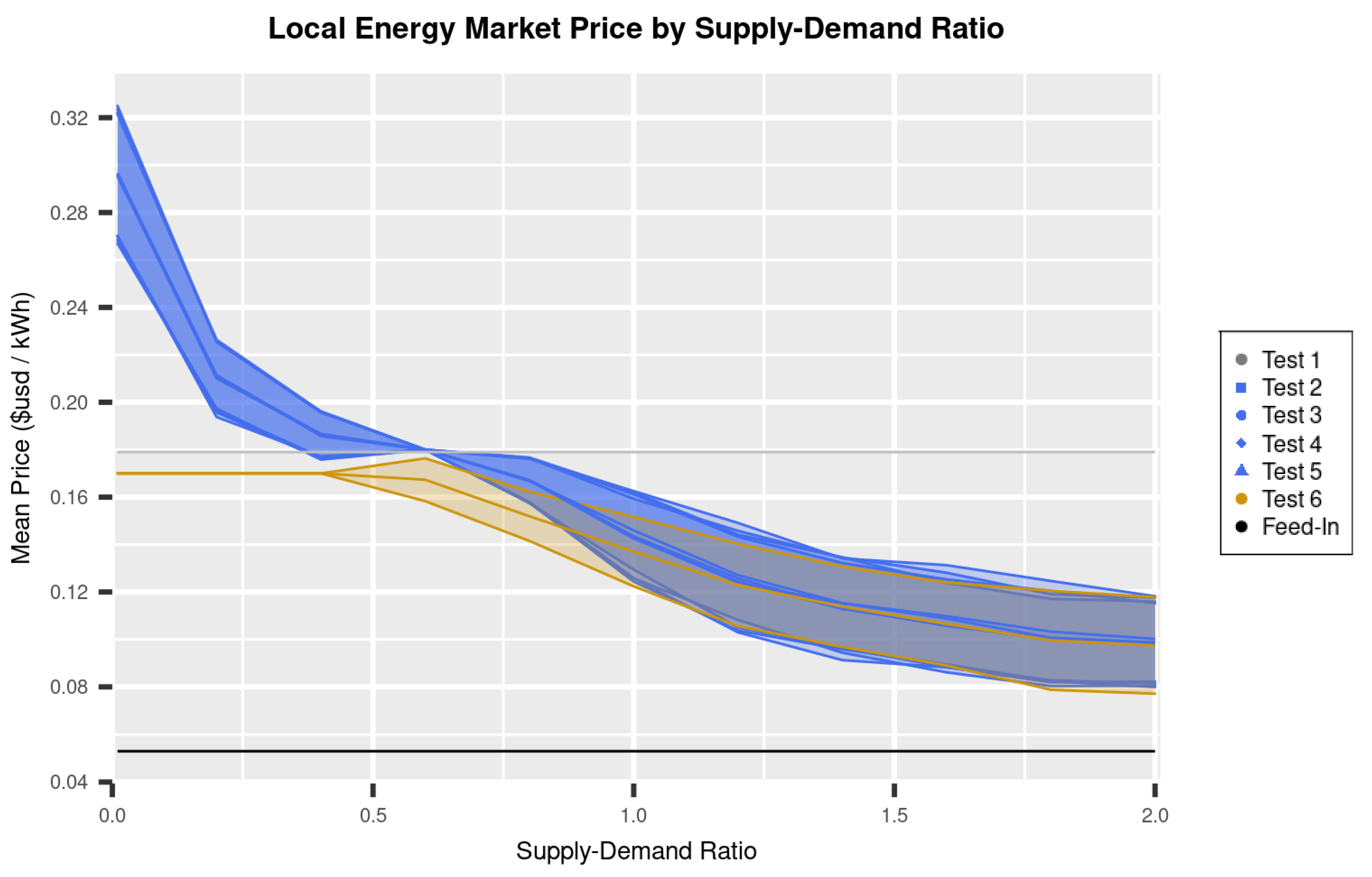
4.1. Local Market Price

The LEM price outcomes in Figure 2 suggest that IP agents produce higher price expectations in the UDA market, compared to the “identical” agents simulated in [11,16]. Price expectations are also higher than the retail market price in low-SDR scenarios without price restriction (i.e., Experiment 1, where$K=True$). When $SDR \ge 0.6$, prices produced in simulation experiments were consistent with previous work; however, as SDR increases, prices in Tests 2–6 fall more slowly than previous tests [16], resulting in prices approximately $0.02/kWh higher in the current tests. When $SDR \le 0.6$, Tests 2–5 produce prices considerably higher than the retail market price. Prices are nearly $0.04/kWh higher in these tests, on average, compared to the retail price. As SDR increases towards 0.6, LEM price$p_{loc }$converges to the local retail price$p_{ret}$from above.

Pricing outcomes are consistent with current LEM design requirements in [10,36], suggesting an appropriate simulation implementation. Overall, IP agents produce prices consistent with the general expectation that LEM development may improve local energy prices using an auction-based mechanism.

Price increases in low-SDR settings are qualitatively consistent with expected influence of socio-economic factors in agent behavior, due to the higher valuation LEM users are expected to place on energy traded in the local market, compared to on energy traded with the retail utility grid. In simulations, the price increases expected from IP agents produce higher sale profitability for local prosumers; this produces greater generation incentive, and stronger “upward pressure” on LEM supply-base growth, potentially resulting in better local demand matching over time (i.e., more frequent target-SDR market conditions). However, prices greater than retail may significantly reduce LEM platform adoption among potential users; price increases are especially unaffordable and economically irrational for low income users and may conflict with the expected preferences of potential LEM users from a range of income backgrounds [1,10,11,30].

For each test presented in Figure 2, middle lines within a colored region show the mean LEM price sampled ($\mu \left[MMP\right]$) in an SDR scenario; upper and lower lines on colored regions indicate$\mu \left[MMP\right]+/- \sigma \left[MMP\right]$values. The unweighted mean of some vector x is indicated by$\mu \left[x\right]$, while$\sigma \left[x\right]$gives standard deviation. Feed-in tariff $p_{fit }$is noted in black, and Test 1 retail price $p_{ret}$is noted in gray.

Brooklyn Microgrid users are said to have reported increases in derived utility for energy transactions [37]; but at the same time, local market prices have reportedly not decreased in comparison to retail market prices. Based on this report and given factors such as project messaging towards local households [38], the spatial conditions of the Brooklyn Microgrid area, and the reportedly low prosumer: consumer ratio in current LEM platform trials [34], low-SDR states may currently be prevalent in market settlements. In this case, the results of Tests 2–5 may explain currently-observed market outcomes, and may provide an estimate of LEM outcomes as platform adoption grows in the DES area. Energy prices in the LEM are notably improved in all target-SDR simulation scenarios, compared to the retail market. Previous studies using “identical” agents expect overall price reductions compared to the retail market, as a result of LEM participation; the results of Tests 2–6 confirm that IP agents, which more closely resemble expected real-world users, may also be expected to find lower energy prices in a LEM with average SDR > 0.6, in addition to qualitative utility improvements from LEM use.

4.2. Agent Rationality and Market Efficiency

For all agents in Tests 2–6, rational market participation is satisfied (Table 6). Market efficiency results appear improved compared to previous simulation-based analyses of auction-based LEMs, e.g., [11,13,21], and rationality results are consistent with [16]. Both rationality and efficiency are satisfied by the “baseline” retail market simulated in Test 1, consistent with theoretical expectations for energy infrastructure operation. In Experiment 1 (Tests 2–5), prosumer preference type distribution$\Pi$does not appear to be an influential factor in LEM outcomes; note that this result may vary, as the gap is reduced between$p_{ret}$and$p_{fit}$.

Table 6. Agent rationality (ARA) and market efficiency (EME) results from tests included in Experiments 1 and 2. In the current study, these are taken as validation metrics, as they are theoretically-expected for the auction mechanism simulated.

Validation Metrics for Simulation Implementation
Range	Agent Rationality (ARA)						Market Efficiency (TME)
	Test 1	Test 2	Test 3	Test 4	Test 5	Test 6	Test 1	Test 2	Test 3	Test 4	Test 5	Test 6
Low-SDR	<na>	1	1	1	1	1	1	1	1	1	1	1
Target-SDR	<na>	1	1	1	1	1	1	0.97	0.97	0.97	0.97	0.95
High-SDR	<na>	1	1	1	1	1	1	1	1	1	1	1

Table 6. Agent rationality (ARA) and market efficiency (EME) results from tests included in Experiments 1 and 2. In the current study, these are taken as validation metrics, as they are theoretically-expected for the auction mechanism simulated.

Validation Metrics for Simulation Implementation
Range	Agent Rationality (ARA)						Market Efficiency (TME)
	Test 1	Test 2	Test 3	Test 4	Test 5	Test 6	Test 1	Test 2	Test 3	Test 4	Test 5	Test 6
Low-SDR	<na>	1	1	1	1	1	1	1	1	1	1	1
Target-SDR	<na>	1	1	1	1	1	1	0.97	0.97	0.97	0.97	0.95
High-SDR	<na>	1	1	1	1	1	1	1	1	1	1	1

In theory, the UDA mechanism is expected to maximize technical market efficiency [13,29] and produce rational participation for all agents. At the local level, market efficiency generally refers to supply-demand matching—but under the current TME metric, efficiency may be tested within each SDR scenario. While efficiency results in Tests 2–6 are consistent with [16], and appear higher than [11], target-SDR results suggest that a more dynamic approach to MRE learning parameter tuning may further improve market efficiency; for example, one that derives SDR-specific values, and/or fully-individualized values for each agent. As current results are near-optimal under a single static parameter tuning, it is suggested that future work may explore convergence speed and outcome stability for the MRE algorithm in more detail, relative to other learning approaches for LEM platform software implementation.

4.3. Consumers’ Relative Market Access

The IP agents show strong differences in market outcomes among consumers in low-SDR scenarios along lines of household income and value preferences in Tests 2–5. Households’ LEM access disparities are eliminated from these scenarios in Test 6, compared to Tests 2–5 (Figure 3). This suggests that a differential willingness and ability (between consumers) to pay for LEM energy may mediate access disparities produced by auction-based settlement mechanisms. The market access disparities described in Figure 3 are similar in shape and magnitude to previous work [16]. In the current work, however, these disparities appear to emerge along lines of modeled income and preference inequality. In the previous work, results were produced with parameters ${\theta }_i=1 \forall i \in I$ and $p_{loc} \in \{p_{fit},p_{ret}\}$.

Figure 3. Relative market access for consumers (RMAc) and prosumers (RMAp), separated by test and SDR range.

Figure 3. Relative market access for consumers (RMAc) and prosumers (RMAp), separated by test and SDR range.

Due to rationality constraints, consumer preferences are indirectly shaped by income. However, income does not fully determine preference under the current model—rather, income constrains the the rational range of potential market preference expression, given financial conditions. Under rationality constraints on consumers’ bidding range, middle-income agents (Con 2, 3) become both willing and able to bid more than higher-income agents (Con 4–6), despite the latter having the economically-rational ability to express much greater “alternative” value preference $(1-{\theta }_i)$, and “ability to pay”. Accordingly, Con 3 consumers (middle-income, medium “alternative” preference) may be able to secure higher access than other consumer groups in a UDA-based LEM. Across all consumers, the RMAc gap between own-economic preference outcomes and “alternative” preference outcomes is between 20–40%. In other words, consumers who are both willing and able to rationally express “alternative” energy value preferences in the market place may use strategies which produce between 20–40% higher market access (compared to highest observed) under simulated conditions.

This result is produced by a merit-order supply allocation in UDA mechanism design, in which higher-bidding consumers are preferentially matched with local supply. This technique is desirable for its production of allocative efficiency in markets for private goods, but appears theoretically incompatible with the access goals of energy distribution infrastructure. By comparison, Figure 3 indicates that fully-uniform market access is produced by the baseline retail market scenario in Test 1; this result is consistent with expected operating conditions of utility-scale energy infrastructure. Results suggest further research on LEM mechanisms which can be expected to maintain market access standards for utility customers, and suggest that auction-based LEMs without price restriction may not be suitable for main roles in energy distribution infrastructure. At the same time, consumer access disparities are reduced in target-SDR scenarios, with remaining market access reductions being distributed near-uniformly among consumer groups. These remaining access reductions may be supported by sub-optimal market efficiency.

Experiment 2 results (Test 6) show that consumer market access disparities in low-SDR conditions may be eliminating by requiring agent strategies$S{\prime }_{i,t} \in \{p_{fit},p_{ret}\}$. Under merit-order supply allocation, unrestricted pricing provide a larger range of strategies for users who are rationally able and willing to place higher bids, thereby allowing a user agent to secure higher market access more consistently. When bidding is restricted to a range which is rationally-feasible for all consumers, market competition is increased, and the ability of consumer agents to distinguish their bids from others is reduced. Accordingly, the average level of market access experienced by individual consumers becomes more consistent, and becomes disconnected from socio-economic disparities. Future work may therefore benefit from further extension of [16] to analyze potential differences in outcome stability across time for IP agents.

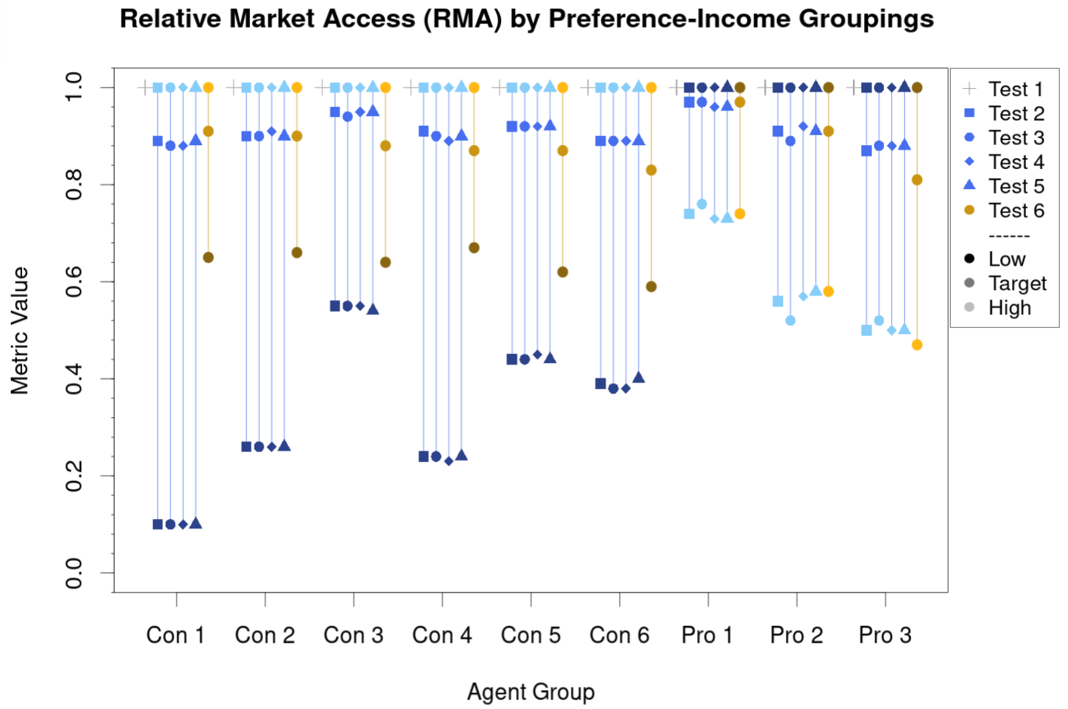
4.4. Prosumers’ Relative Market Access

The market access disparities shown for prosumers in Figure 3 are consistent with [16], and further indicate that prosumers with higher sensitivity to decreases in local market price may select market strategies which increase their market share compared to other prosumers. With increasing${\theta }_i$, prosumers derive greater value from LEM sales at lower prices; this potentially enables them to rationally provide lower prices than their peers, and gain preferential matching with local consumers via merit-order supply allocation. However, the opposite result is seen in prosumer RMA: RMAp disparities begin to grow as$SDR \to 1$, and continue to expand as SDR increases into the “high-SDR” range.

As SDR increases, an increasingly-wide gap is produced between outcomes for prosumers that secure sale matches locally, versus prosumers who do not. In other words, the gap between sale profits without LEM matching, versus with LEM matching, show a strong positive correlation with SDR. This indicates that prosumer access disparities may be produced by differences in market strategy learning adaptation, which may result from differences in prosumers’ utility function sensitivity to changes in the multi-agent “environment” which produces LEM conditions—for example, sensitivity to LEM price fluctuations.

In short, current results suggest that price-sensitive prosumer agents may be expected to outperform price-inelastic prosumers—whom, in theory, may be satisfied by market strategies low enough to undercut their peers. On LEM platforms which require direct user input of market strategies, these results suggest that prosumers which are more actively engaged in market strategy adaptation on the LEM platform may be expected to secure greater market share. Despite that RMA is a socio-economic metric, this does not necessarily suggest a clear equity conflict in prosumer outcomes in the simulated UDA market.

Based on the prosumer results in Figure 3, a given utility function may produce more effective learning stimulus than another under the MRE algorithm, in a given learning environment where identical and constant values of$\lambda$and$ϵ$are used for all agents. It is also noted that these RMAp results may be affected by MRE learning parameter tuning; just as utility function sensitivity to changes in market conditions appear to impact effective learning adaptation, learning parameters$\lambda$and$ϵ$may modulate agent learning. Accordingly, future work may consider deriving more individualized parameter tunings at the agent level.

This implies that we can expect similar behavioral phenomena for consumers, suggesting that consumers with lower${\theta }_{i }$values are expected to be less sensitive to local price changes, while consumers with higher${\theta }_i$may be expected to produce more price-sensitive behaviors. However, this is consistent with the interpretation of consumer${\theta }_i$as modeling “willingness to pay”, constrained by “ability to pay” offered in Section 2.4. Accordingly, the results described in Figure 3 are also considered interpretable for real-world user agents, based on the current modeling interpretation. Further analysis may aim to disaggregate the impact of learning disparities on consumer outcomes from that of market settlement dynamics.

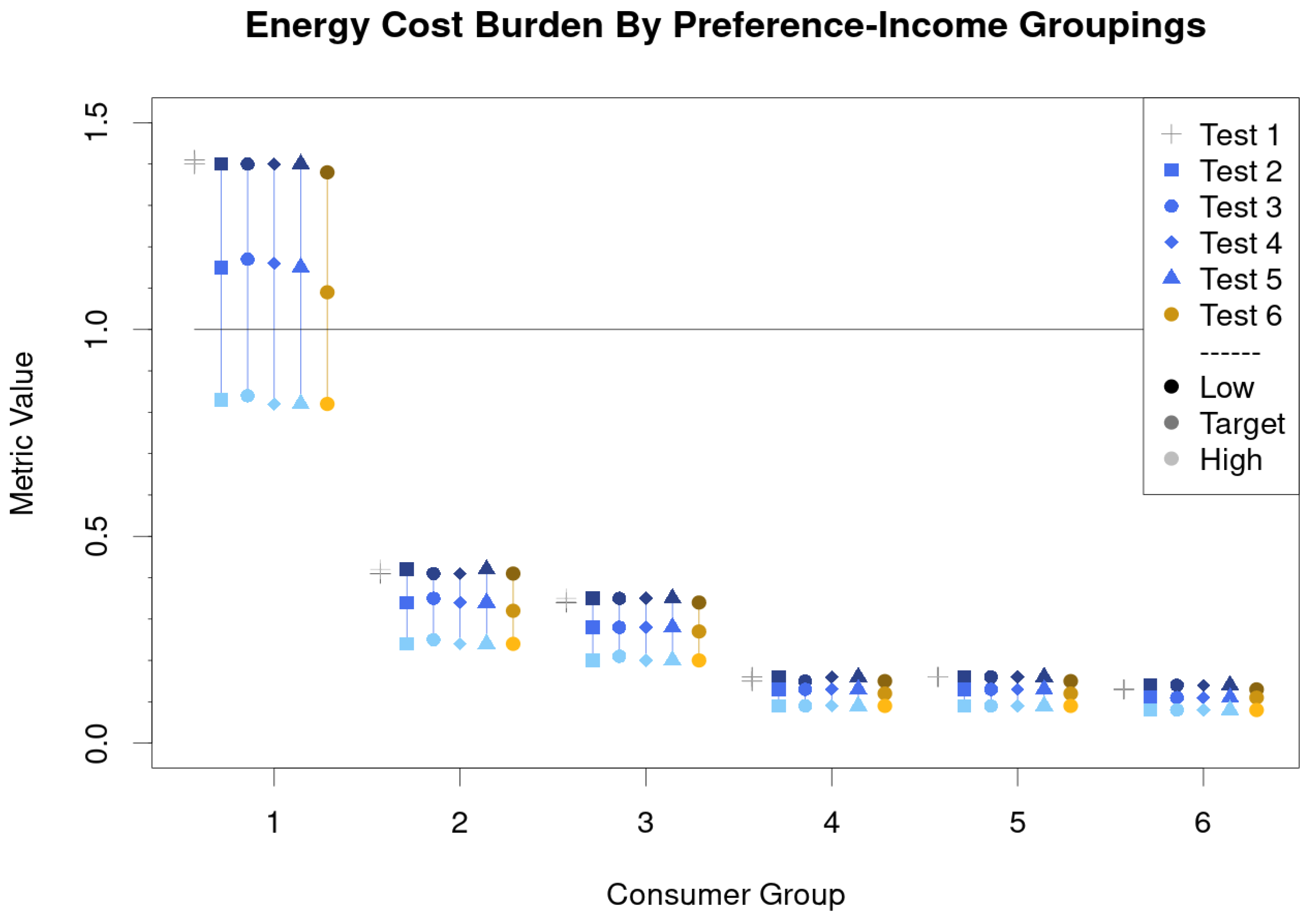
4.5. Energy Cost Burden

Energy affordability was improved by LEM operation in target-SDR and high-SDR ranges of Tests 2.6 compared to the baseline retail market simulated in Test 1 (Figure 4). In these cases, greater market access for lower-income groups led to notable reductions in local outstanding energy cost burden. With the exception of low-income consumers (Con 1), agents’ energy costs in all tests are affordable, requiring less than 3% of agents’ income ($R_i$). For Con 1, energy costs remained unaffordable in low-SDR and target-SDR scenarios, with costs as high as ~140% and ~115%, respectively, of their individually affordable energy cost.

In low-SDR scenarios, considerable price increases above$p_{ret}$are produced in the local market; in these cases, energy cost burdens for low-income consumers would not be reduced by LEM operation, compared to the baseline retail market (Test 1), even if uniform RMAc was achieved. Results are consistent across all tests in Experiment 1, further confirming a lack of sensitivity to the local prosumer preference distribution$\Pi$in local market outcomes. In comparison with Tests 2–5 results, Test 6 results indicate that low-SDR energy affordability gaps are only slightly reduced by local price restriction, despite the production of more uniform market access among consumers.

In target-SDR conditions, a greater reduction in ECB is noted for Test 6, resulting in low-income ECB which is at least 10% higher, on average, than what households can afford to pay (i.e., 110%). For all other consumer groups, ECB is no greater than 40% in any test presented here in comparison to mean observed ECB values of 48% in New York City overall [1]. We note that these results may be conservative, based on the current modeling; real ECB values may be even higher.

In low-SDR settings, simulated energy burden outcomes from LEM and retail markets are similar for low-income consumers, and are consistent with empirical data. In New York City, for example, the cited work estimates that at least 50% of low-income households experience energy burdens greater than 9%, with energy burden reaching nearly 18% of income for at least 25% of low-income households. These outcomes are neither uncommon nor the most severe, in the context of metro areas in the United States today. Low-income energy burden in the U.S. overall may be above 7%; for comparison, the average remaining energy cost burden for low-income consumers in low-SDR and target-SDR conditions is ~8.4% and ~6.9%, respectively (across Tests 2–6). An ECB of 6% is considered affordable locally ($e\prime$).

Relatively small ECB differences are seen between consumer groups with varying${\theta }_i$. Con 2 and Con 3 ECB varies by 10%; Con 5 and Con 6 vary by just 5%; Con 1 and Con 2, however, have a relative difference of ~100%. Individually, ECB can be seen as a function of income ($R_i$) and local market quantity ($Q_{con,loc}$), as simulated energy price and demand are held uniform among consumers. As locally-secured energy quantity goes down, quantity purchased at retail price goes up to compensate; therefore, a correlation between RMA and ECB might be expected. However, this correlation is not apparent in current results, possibly suggesting a non-linear relationship. In any case, further analysis may extend current understanding of market dynamics under the simulated UDA mechanism.

5. Conclusions & Future Work

Simulation results are consistent with many expectations from previous works, and with theoretical expectations for techno-economic outcomes of double-sided auction market mechanisms. Consistent with previous works, LEM operation is expected to produce energy prices which greatly improve sale profitability for local prosumers, while also reducing energy prices for local consumers, compared to the retail utility market. Market efficiency results for IP agents suggest that a more dynamic approach to MRE parameter tuning may produce behavior suitable for use in LEM software agents, depending on the results of follow-up tests for algorithm convergence speed and outcome stability.

In LEM settlements with a low supply-demand ratio (SDR), however, market access issues may emerge under UDA market design which are not observed in the baseline energy market scenario. In addition, while energy affordability is expected to improve under LEM operation, the current results do not expect the elimination of energy affordability issues for low-income households under low-SDR or target-SDR conditions. Results show that restricting LEM prices to the range between$p_{fit}$ and$p_{ret }$may effectively eliminate market access disparities between consumers; however, they also suggest that market access improvements may not greatly improve energy affordability outcomes compared to unrestricted pricing (with the latter producing stronger LEM price incentives for prosumers in low-SDRs).

While emergent disparities in prosumers’ market access may provide insight on effective supply-side LEM behaviors, consumer results suggest against using auction-based LEMs with non-trivial local income and/or value preference inequality. The expectation of continued low-income energy insecurity under LEM operation, and the observed mapping of market access disparities from previous work to local inequalities modeled in the present work, suggest that current auction-based mechanisms may not be appropriate for use in low-income settings.

Auction-based mechanisms may significantly improve cost affordability and sale profitability for LEM users overall, but low-income users may see minimal value in LEM participation in the majority of SDR conditions evaluated—suggesting that auction-based LEMs may require continued external investments in local energy affordability programs for consumers, or cost subsidy programs aimed at remaining local energy affordability gaps. An individually rational LEM mechanism which consistently addresses energy access and affordability issues may support reductions in overall expenses for energy distribution infrastructure operations. This goal may be especially relevant to municipal energy utilities.

The current study simplifies a number of LEM operation factors; a once-daily market settlement is considered, agents’ supply and demand are static and uniform across same-type agents, and prosumer energy storage is not modeled. These decisions allow for clearer observation of mechanism design dynamics and their impacts, by reducing the number of variable parameters. At the same time, the simplicity of the current simulation environment may reduce the direct applicability of results to a specific LEM operation scenario. As exogenous factors are modeled more fully, and as LEM settlement data becomes more widely available, greater accuracy and detail can be produced for specific platforms LEM platforms. We note, however, that the ability of such studies to comment on a mechanism design itself may be reduced.

It is strongly recommended that socio-economic evaluation metrics should be derived from established theoretical foundations. In the environmental justice literature, an ethical analysis approach based on fairness-justice criteria has been developed to analyze socio-economic outcomes through an “energy equity” scope, consistent with emerging “equitable” impact standards for energy industry. The socio-economic results metrics in this current work represent necessary components of equity analysis, but are not yet minimally-sufficient for equity analysis by themselves. At minimum, a measure of agents’ temporal outcome stability is needed. Overall, the current study presents foundational steps toward normalizing LEM mechanism analysis in a more complete socio-technical context.

6. Glossary of Symbols and Abbreviations

This section gives an overview of parameter notation presented in the previous sections of the paper (see

Table 7. Overview of key simulation parameters.

Simulation Parameters
Name	Initialization	Description
Set of simulation steps	$T= \{1,2,3,\dots ,365\}$	Local and retail markets settled once per step
Agent index numbers	$\begin{array}{c}I= \{I_{con},I_{pro}\}\\ = \{1, \dots , 100\}\end{array}$	$I_{con}$ ← Consumer agent indices $I_{pro}$ ← Prosumer agent indices
Number of consumers	$|I_{con}| =75$	75 consumer agents selected at initialization (Section 2.4)
Number of prosumers	$|I_{pro}| =25$	25 consumer agents selected at initialization (Section 2.4)
Grid feed-in tariff	$p_{fit}=$$0.053 USD/kWh	(Section 2.1)
Grid retail price	$p_{ret}=$$0.175 USD/kWh	(Section 2.1)
Agent daily demand	$D_i= 19.64 \mathrm{kWh} \forall i \in I$	(Section 3)
Agent daily generation	Function of variable parameter Set based on current SDR value (Section 3.1)	$\mathrm{For} \mathrm{each} i \in I$: $\mathrm{If} (C_i=0$): $G_i=D_i+\frac{SDR \ast \left( {\sum }_{j\in I_{\mathit{con}}}{D}_j \right)}{\left|I_{pro}\right|}$ $\mathrm{Else}: G_i=0$
Equitable supply threshold	$EST=\mu [ D_{i \in I} ]$	(Section 2.6)
Minimum agent income	$r_{min}$ = $10,000 USD/year	(Section 2.1)
Maximum agent income	$r_{max}$ = $200,000 USD/year	(Section 2.1)
Agent incomes	Set by random distribution	(Section 2.1)
Locally-defined threshold for affordable energy cost	$e\prime =0.06$	6% of income is considered affordable locally (Section 2.4, Section 2.6)
Locally-observed “high” energy cost burden	$e_{obs}=0.13$ $(\mathrm{note}: e_{obs} \gg e’$)	$\mathrm{Energy} \mathrm{bills} \mathrm{above} 13\% \mathrm{of} \mathrm{income} \mathrm{are} \mathrm{observed} \mathrm{locally}; \mathrm{taken} \mathrm{as} \mathrm{upper}-\mathrm{limit} \mathrm{to} “\mathrm{willingness} \mathrm{to} \mathrm{pay}” \mathrm{for} \mathrm{agents}’ S_i$ initialization (Section 2.4)
Consumers’ individually affordable energy prices	$\mathrm{For} \mathrm{each} i \in I_{con}$: $P_i^{\ast }=\frac{\left(R_i/|T|\right) \ast e’}{EST}$	(Section 2.4)
Agent is “consumer”?	$C_i \in \{true, false\} \forall i \in I$	Set of Boolean values indicating agent “type” (Section 3)
Learning “memory”	$ϵ=0.01$	(Section 2.5)
Learning “rate”	$\lambda =0.083$	(Section 2.5)
Agent utility preferences	Consumer: ${\theta }_{con, i} \in \left[0,1\right]$ Prosumer: ${\theta }_{pro, i} \in \{1, 2, 3\}$	Consumer: own-economic utility preference Prosumer: utility preference “type” (Section 2.2, Section 2.3 and Section 2.4)
Market mechanism	$\mathrm{Mapping} \mathrm{from} \{S{’}_t, Q_{0,t}\}$ $\mathrm{to} \{ P_{loc,t}, Q_{loc,t} \}$$, \mathrm{for} t \in T$	(Section 2.1, Section 3) Experiment 0 Parameter
Prosumer type distribution	$\Pi = \{ {\pi }_1, {\pi }_2, {\pi }_3 \}$ Where: ${\pi }_{j \in \{1,2,3\}}=Prob\left({\theta }_i=j \right)$ $\mathrm{And}: \left({\sum }_{\mathrm{j}\in \left\{1,2,3\right\}}{\pi }_j\right)=1$	(Section 3.1) Experiment 1 Parameter
Local price constraint?	$\mathrm{Is} p_{loc,t} \in [p_{fit}, p_{ret}]$ required in the LEM at each time step? $\mathrm{Noted} \mathrm{by}: K \in \{true, false\}$	(Section 3.1) Experiment 2 Parameter
Market supply-demand ratio (SDR)	Variable parameter for all modeling scenarios tested (Section 3.1)	$SDR= \{ 0.01, 0.1, 0.2, 0.3, \dots , 1.0, \dots , 2.0 \}$ $\mathrm{Determines} \mathrm{prosumer} G_i\forall i \in I_{pro}$

and

Table 8. Overview of model output data from simulated marketplace.

Market Data Notation
Variable	Description
$P_{i,t}$	$\mathrm{Set} \mathrm{of} \mathrm{prices} \mathrm{for} \mathrm{each} \mathrm{agent} \mathrm{at} \mathrm{step} t \in T$ $\mathrm{Each} \mathrm{element} \mathrm{is} P_{i,t}=\{P_{loc,i,t },P_{ret,i,t}\}$$\mathrm{for} \mathrm{some} i \in I$$\mathrm{and} t \in T$
$P_{loc,t}$	$\mathrm{Local} \mathrm{market} \mathrm{prices} (\mathrm{for} \mathrm{each} \mathrm{agent}) \mathrm{at} \mathrm{step} t \in T$ $\mathrm{Each} \mathrm{element} \mathrm{of} P_{loc,t}=\{P_{loc,con,t} ,P_{loc,pro,t}\}$ holds consumer costs and prosumer sales
$P_{ret,t}$	$\mathrm{Retail} \mathrm{market} \mathrm{prices} (\mathrm{for} \mathrm{each} \mathrm{agent}) \mathrm{at} \mathrm{step} t \in T$$, \mathrm{such} \mathrm{that} P_{ret,t}= \{P_{ret,con,t},P_{ret,pro,t}\}$. $\mathrm{Each} \mathrm{element} P_{ret,con,t}=p_{ret}$$\mathrm{for} i \in I_{con}$$, \mathrm{and} \mathrm{each} P_{ret,pro,t}=p_{fit}$$\mathrm{for} i \in I_{pro}$
$Q_{i,t}$	$\mathrm{Individual} \mathrm{market} \mathrm{return} \mathrm{quantities} \mathrm{at} \mathrm{step} t \in T$ $\mathrm{Each} \mathrm{element} \mathrm{is} Q_{i,t}=\{Q_{loc,i,t },Q_{ret,i,t}\}$$\mathrm{for} \mathrm{some} i \in I$$, t \in T$
$Q_{loc,t}$	$\mathrm{Consumers}’ \mathrm{local} \mathrm{energy} \mathrm{purchase} \mathrm{quantities} \mathrm{at} \mathrm{step} t \in T$ $\mathrm{Each} \mathrm{element} \mathrm{of} Q_{loc,t}=\{Q_{loc,con,t} ,Q_{loc,pro,t}\}$ holds agents’ local purchase and sale quantities
$Q_{ret,t}$	$\mathrm{Prosumers}’ \mathrm{local} \mathrm{energy} \mathrm{sale} \mathrm{quantities} \mathrm{at} \mathrm{step} t \in T$ $\mathrm{Each} \mathrm{element} \mathrm{of} Q_{ret,t}=\{Q_{ret,con,t} ,Q_{ret,pro,t}\}$ holds agents’ retail purchase and sale quantities
$Q_{0,t}$	$\mathrm{Agents}’ \mathrm{initial} \mathrm{supply} \mathrm{or} \mathrm{demand} \mathrm{quantities} \mathrm{at} \mathrm{step} t \in T$ $\mathrm{Each} \mathrm{element} \mathrm{of} Q_{0,t}=\{Q_{0,con,t },Q_{0,pro,t}\}$ holds agents’ initial demand and supply quantities
$S{’}_t$	$\mathrm{Agents}’ \mathrm{selected} \mathrm{market} \mathrm{strategies} \mathrm{for} \mathrm{step} t \in T$ $\mathrm{Each} \mathrm{element} S{’}_{i,t}$$\mathrm{holds} \mathrm{the} \mathrm{submitted} \mathrm{price} \mathrm{strategy} \mathrm{of} \mathrm{agent} i \in I$$\mathrm{at} \mathrm{time} t \in T$

). Description of LEM input and output data is also provided to help clarify the process of agent learning and results derivation.

References

1. Drehobl, A.; Ross, L.; Ayala, R. How High Are Household Energy Burdens? An Assessment of National and Metropolitan Energy Burden across the United States; ACEEE: Washington, WA, USA, 2020. [Google Scholar]
2. Wang, F.; Harindintwali, J.D.; Yuan, Z.; Wang, M.; Li, S.; Yin, Z.; Huang, L.; Fu, Y.; Li, L.; Chang, S.X.; et al. Technologies and perspectives for achieving carbon neutrality. Innovation 2021, 2, 100180. [Google Scholar] [CrossRef] [PubMed]
3. Tushar, W.; Saha, T.K.; Yuen, C.; Smith, D.; Poor, H.V. Peer-to-Peer Trading in Electricity Networks: An Overview. IEEE Trans. Smart Grid 2020, 11, 3185–3200. [Google Scholar] [CrossRef] [Green Version]
4. Staudt, P.; Köpje, S.; Weinhardt, C. Market mechanisms for neighbourhood electricity grids: Design and agent-based evaluation. In Proceedings of the 27th European Conference on Information Systems—Information Systems in a Sharing Society ECIS 2019, Stockholm, Sweden, 8 June 2019; pp. 1–16. [Google Scholar]
5. Khorasany, M.; Mishra, Y.; Ledwich, G. Market framework for local energy trading: A review of potential designs and market clearing approaches. IET Gener. Transm. Distrib. 2018, 12, 5899–5908. [Google Scholar] [CrossRef] [Green Version]
6. Georgarakis, E.; Bauwens, T.; Pronk, A.-M.; AlSkaif, T. Keep it green, simple and socially fair: A choice experiment on prosumers’ preferences for peer-to-peer electricity trading in the Netherlands. Energy Policy 2021, 159, 112615. [Google Scholar] [CrossRef]
7. Wörner, A.M.; Ableitner, L.; Meeuw, A.; Wortmann, F.; Tiefenbeck, V. Peer-to-Peer Energy Trading in the Real World: Market Design and Evaluation of the User Value Proposition. In Proceedings of the 40th International Conference on Information Systems ICIS 2019, Munich, Germany, 15–18 December 2019. [Google Scholar] [CrossRef]
8. Wilkins, D.J.; Chitchyan, R.; Levine, M. Peer-to-Peer Energy Markets: Understanding the Values of Collective and Community Trading. In Proceedings of the 2020 CHI Conference on Human Factors in Computing Systems, New York, NY, USA, 25 April 2020. [Google Scholar] [CrossRef]
9. Wilkinson, S.; Hojckova, K.; Eon, C.; Morrison, G.M.; Sandén, B. Is peer-to-peer electricity trading empowering users? Evidence on motivations and roles in a prosumer business model trial in Australia. Energy Res. Soc. Sci. 2020, 66, 101500. [Google Scholar] [CrossRef]
10. Mengelkamp, E.; Gärttner, J.; Rock, K.; Kessler, S.; Orsini, L.; Weinhardt, C. Designing microgrid energy markets: A case study: The Brooklyn Microgrid. Appl. Energy 2018, 210, 870–880. [Google Scholar] [CrossRef]
11. Mengelkamp, E.; Staudt, P.; Garttner, J.; Weinhardt, C. Trading on local energy markets: A comparison of market designs and bidding strategies. In Proceedings of the 2017 14th International Conference on the European Energy Market (EEM), Dresden, Germany, 6–9 June 2017. [Google Scholar] [CrossRef]
12. El-Baz, W.; Tzscheutschler, P.; Wagner, U. Evaluation of energy market platforms potential in microgrids: Scenario analysis based on a double-sided auction. Front. Energy Res. 2019, 7, 41. [Google Scholar] [CrossRef]
13. Lin, J.; Pipattanasomporn, M.; Rahman, S. Comparative analysis of auction mechanisms and bidding strategies for P2P solar transactive energy markets. Appl. Energy 2019, 255, 113687. [Google Scholar] [CrossRef]
14. Parag, Y.; Sovacool, B.K. Electricity market design for the prosumer era. Nat. Energy 2016, 1, 1–6. [Google Scholar] [CrossRef]
15. New York City. Understanding and Alleviating Energy Cost Burden in New York City. 2019. Available online: https://www1.nyc.gov/assets/sustainability/downloads/pdf/publications/EnergyCost.pdf (accessed on 8 June 2022).
16. Beattie, S.; Chan, W.-K.V. Broadening the Scope of Analysis for Peer-to-Peer Local Energy Markets to Improve Design Evaluations: An Agent-Based Simulation Approach. In Lecture Notes in Operations Research; Springer International Publishing: Cham, Switzerland, 2021; pp. 238–253. [Google Scholar]
17. US Census. 2019—New York–Kings County—Brooklyn Borough. Am. Commun. Surv. 2019. Available online: https://data.census.gov/cedsci/table?t=IncomeandPoverty&g=0600000US3604710022&tid=ACSST5Y2019.S1901 (accessed on 7 July 2021).
18. Zhou, Y.; Wu, J.; Long, C.; Cheng, M.; Zhang, C. Performance Evaluation of Peer-to-Peer Energy Sharing Models. Energy Procedia 2017, 143, 817–822. [Google Scholar] [CrossRef]
19. Zhou, Y.; Wu, J.; Long, C. Evaluation of peer-to-peer energy sharing mechanisms based on a multiagent simulation framework. Appl. Energy 2018, 222, 993–1022. [Google Scholar] [CrossRef]
20. Zhou, Y. Peer-to-Peer Energy Trading in Microgrids and Local Energy Systems; Jenkins, J.W.E.-N., Ed.; IntechOpen: Rijeka, Croatia, 2021; Chapter 3. [Google Scholar]
21. Nicolaisen, J.; Petrov, V.; Tesfatsion, L. Market power and efficiency in a computational electricity market with discriminatory double-auction pricing. IEEE Trans. Evol. Comput. 2001, 5, 504–523. [Google Scholar] [CrossRef] [Green Version]
22. Ableitner, L.; Tiefenbeck, V.; Meeuw, A.; Wörner, A.; Fleisch, E.; Wortmann, F. User behavior in a real-world peer-to-peer electricity market. Appl. Energy 2020, 270, 115061. [Google Scholar] [CrossRef]
23. Ecker, F.; Spada, H.; Hahnel, U.J.J. Independence without control: Autarky outperforms autonomy benefits in the adoption of private energy storage systems. Energy Policy 2018, 122, 214–228. [Google Scholar] [CrossRef]
24. Hahnel, U.J.J.; Herberz, M.; Pena-Bello, A.; Parra, D.; Brosch, T. Becoming prosumer: Revealing trading preferences and decision-making strategies in peer-to-peer energy communities. Energy Policy 2020, 137, 111098. [Google Scholar] [CrossRef]
25. Frank, M.; Colgrove, M.; Martin, C.; Levin, E.; Palchak, E.; Stephenson, R. Towards Standardized Equity Measurement in the Clean Energy Industry: Work Plan and Literature Reveiws. Available online: https://www.veic.org/Media/default/documents/resources/reports/equity_measurement_clean_energyindustry.pdf (accessed on 7 September 2019).
26. McCauley, D.A.; Heffron, R.J.; Stephan, H.; Jenkins, K. Advancing energy justice: The triumvirate of tenets. Int. Energy Law Rev. 2013, 32, 107–110. [Google Scholar]
27. Sovacool, B.K.; Dworkin, M.H. Energy justice: Conceptual insights and practical applications. Appl. Energy 2015, 142, 435–444. [Google Scholar] [CrossRef]
28. Erev, I.; Roth, A.E. Predicting how people play games: Reinforcement learning in experimental games with unique, mixed strategy equilibria. Am. Econ. Rev. 1998, 88, 848–881. [Google Scholar]
29. Narahari, Y. Game Theory and Mechanism Design; World Scientific Publishing Company; Indian Institute of Science: Bangalore, India, 2014. [Google Scholar]
30. Xu, X.; Chen, C. Energy efficiency and energy justice for US low-income households: An analysis of multifaceted challenges and potential. Energy Policy 2019, 128, 763–774. [Google Scholar] [CrossRef]
31. Kontokosta, C.E.; Reina, V.J.; Bonczak, B. Energy cost burdens for low-income and minority households: Evidence from energy benchmarking and audit data in five US cities. J. Am. Plan. Assoc. 2020, 86, 89–105. [Google Scholar] [CrossRef]
32. Fisher Sheehan Colton Public Finance General Economics. Home Energy Affordability Gap. 2021. Available online: http://homeenergyaffordabilitygap.com/01_whatIsHEAG2.html (accessed on 20 January 2022).
33. New York Energy Ratings, Electricity Rates and Usage for Brooklyn, New York. 2019. Available online: https://www.nyenergyratings.com/electricity-rates/new-york/brooklyn (accessed on 7 July 2021).
34. Sharma, R.; Brooklyn Microgrid Gets Approval for Blockchain-based Energy Trading. Energy Central. 2019. Available online: https://energycentral.com/c/iu/brooklyn-microgrid-gets-approval-blockchain-based-energy-trading (accessed on 1 May 2022).
35. New York City, Deriving a Poverty Threshold for New York City. 2020. Available online: https://www1.nyc.gov/assets/opportunity/pdf/NYCgovPoverty2020_Appendix_B.pdf (accessed on 7 July 2021).
36. Block, C.; Neumann, D.; Weinhardt, C. A market mechanism for energy allocation in micro-CHP grids. In Proceedings of the Annual Hawaii International Conference on System Sciences, Waikoloa, HI, USA, 7–10 January 2008; p. 172. [Google Scholar] [CrossRef]
37. Livingston, D.; Sivaram, V.; Freeman, M.; Fiege, M. Applying Blockchain Technology to Decentralized Waste Management. 2018, pp. 2–3. Available online: https://blogs.systweak.com/applying-blockchain-technology-to-waste-management/ (accessed on 20 April 2018).
38. LO3 Energy, Brooklyn Microgrid—About. 2019. Available online: https://www.brooklyn.energy/about (accessed on 7 July 2021).
Figure 1. LEM simulation execution overview at local level; agent-level overview is shown in Section 2.5.
Sustainability 14 07642 g001
Figure 2. Overview of LEM prices across SDR range.
Sustainability 14 07642 g002
Figure 4. Individual-level energy cost burden ECB, separated by test and SDR range.
Sustainability 14 07642 g004