Article

Competition and Heterogeneous Innovation Qualities: Evidence from a Natural Experiment

School of Economics and Resource Management, Beijing Normal University, Beijing 100875, China
*
Author to whom correspondence should be addressed.
Sustainability 2022, 14(13), 7562; https://doi.org/10.3390/su14137562
Submission received: 26 April 2022 / Revised: 11 June 2022 / Accepted: 17 June 2022 / Published: 21 June 2022
(This article belongs to the Topic Open Innovation and Entrepreneurship)

Abstract

:
Innovations differ substantially in their qualities, from major breakthroughs to small incremental refinements. What is the relationship between product market competition and the quality of innovations? We develop a model where competition encourages high-quality firms to innovate but discourages low-quality firms from innovating and examine the impact of competition on the quality of innovations, taking the implementation of the negative list system for market access in China as a natural experiment. It is found that competition has twofold impacts on the incentives of innovation and that competition improves the overall innovation quality through the improvement of innovation resource allocation. More competition implies a higher elasticity of substitution, leading to stronger incentives for innovation. Meanwhile, competition also decreases industry profits and increases the cost of innovation, which reduces the expected return on innovation, resulting in fewer incentives for innovation. The findings suggest that while R&D subsidies increase aggregate R&D investment, they encourage the survival and expansion of low-quality firms at the expense of high-quality firms and lead to misallocation of R&D resources, resulting in the decline of overall innovation qualities.

1. Introduction

It is widely recognized that product competition has a significant impact on R&D investment conducted by private firms and thus on innovation. In practice, innovation is highly heterogeneous across firms, with different economic and technological significance. Although numerous empirical and model-based studies have examined the relationship between competition and aggregate R&D spending, little is known about the impact of competition on heterogeneous innovation qualities. In this paper, we attempt to bridge this gap by studying the effects of competition on innovation in a general equilibrium model, featuring firms with heterogeneous innovation qualities and exploiting the implementation of the negative list system for market access in China as a natural experiment to empirically test the relationship between competition and innovation quality.
Early research on the relationship between competition and innovation can be traced back to Schumpeter [1]. In his book Capitalism, Socialism and Democracy, Schumpeter argues that monopolistic market structures are more conducive to promoting innovation and economic growth than competitive market structures due to the ability of monopolists to attract talent, secure a high financial standing and deploy an array of restrictive practices to protect their investments, while “perfect competition is not only impossible but inferior and has no title to being set up as a model of ideal efficiency.” Since then, the literature on competition and innovation has conducted analysis from three main perspectives.
The first perspective is to contrast the effects of monopolistic and competitive market structure on incentives for innovation. For example, Arrow [2] compares the incentives of monopoly and perfect competition on process innovation and argues that competition increases the rents that firms can obtain from cost-reducing innovations and can provide greater incentives for innovation. A study by Greenstein and Ramey [3] addresses vertical product innovation and argues that monopolists supply both old and new products, which allows the monopolist to carry out price discrimination and leads to higher profits than those of competitive firms that can produce only new products. Therefore, the incentive to carry out vertical product innovation is greater when the product market is monopolistic. The study of Chen and Schwartz [4] on horizontal product innovation also argues that the inability of competitive firms to implement price discrimination leads to greater incentives for monopolists to innovate than competitive firms.
The second perspective is to analyze the impact of competition on R&D investment and therefore on innovation. For example, Aghion et al. [5] argue that competition has both the Schumpeterian effect and the escape-competition effect, leading to an inverted U-shaped relationship between competition and innovation. Bloom et al. [6] examined the impact of Chinese import competition on innovation in European countries and found that Chinese import competition led to increased technical change within firms, which could account for approximately 14% of the overall technical change in Europe between 2000 and 2007. However, Campbell and Mau [7] found no statistically significant relationship between Chinese import competition and patents in European countries after corrections to the specifications of Bloom et al. [6]. Autor et al. [8], on the other hand, examined the impact of Chinese import competition on innovation in the U.S. and found that Chinese import competition caused a significant decline in the R&D investment of U.S. firms.
The third perspective, which is the one we emphasize in this paper, is to introduce innovation heterogeneity in terms of economic and technological significance [9]. Akcigit and Kerr [10] considered the impact of firm size on innovation quality. They showed that firm size distribution affects innovation incentives and generates heterogeneous innovation qualities. Concerning the impact of policies on innovation qualities, Acemoglu et al. [11] argued that industrial policy subsidizing either R&D or the continued operation of incumbents reduces innovation qualities and growth due to the inefficient allocation of R&D resources. Galaasen and Irarrazabal [12] examined the effect of R&D subsidies on innovation heterogeneity. They found that the size-dependent subsidy increases aggregate R&D investment but reduces growth and welfare, while a uniform subsidy stimulates investment, growth and welfare.
In contrast to the literature, this paper studies the impact of competition on heterogeneous innovation qualities. The intuition of this paper is that competition may promote innovation qualities through a strong selection effect: because the expected profits of high-quality firms to innovate are also high, more competition may foster innovation of high-quality firms while deterring low-quality firms from innovating, which in turn improves the efficiency of R&D resource allocation, leading to the improvement of overall innovation qualities.
This paper proceeds as follows. Section 2 presents a model to illustrate the impact of competition on the quality of innovations, theoretically following Lentz and Mortensen [13]. Section 3 outlines the empirical strategy and describes the data used in the analysis. Section 4 reports the baseline results and additional robustness checks. Section 5 offers concluding remarks.

2. Theoretical Framework

To analyze the impact of competition on the quality of innovations, we first explain the incentives for firms to innovate using a general equilibrium model. Then, we consider the entry decision of firms with heterogeneous innovation qualities and explain the effect of competition on the quality of innovations.

2.1. Incentives for Innovation

Suppose that there are n kinds of products in the market. The utility function of households is given by a CES (constant elasticity of substitution) form and the elasticity of substitution is ε. The utility maximization problem for households is
max q i 0 U = i = 1 n q i ε 1 ε ε ε 1 , s . t .   i = 1 n p i q i = m
where q i is the consumption of product i by households, p i is the price of product i, and m is the income of the households. The price index P and product index Q are defined as
P = i = 1 n p i 1 ε 1 1 ε , Q = i = 1 n q i ε 1 ε ε ε 1 .
Then, the demand function for product i can be obtained as q i = p i ε P ε Q , and the price elasticity of demand for every product is ε (proofs are given in Appendix A). Since greater price elasticity of demand indicates a higher level of competition, following Raith [14], we denote competition by the price elasticity of demand. In addition, because monopolistically competitive firms always operate where the price elasticity of demand is greater than 1, we restrict ε > 1 under a monopolistically competitive market structure.
On the supply side of the products, assume that each product is produced by only one monopolistically competitive firm; specifically, product i is produced by firm i. We assume that only one input, measured by x i , is required in production. The total supply of the factor of production is X, while the price of the factor of production is w. Suppose that the price elasticity of input is 0. Thus, the price of input will be determined entirely by the firm’s demand for the factor of production. Furthermore, the production function of firm i is q i = A i x i , where q i is the output and A i denotes the technology of firm i. Therefore, the cost function and the marginal cost of firm i are
c i q i = w x i = w q i A i ,   M C i = d c i d q i = w A i ,
where c i q i is the cost function, and M C i is the marginal cost. We define the technology index reflecting the technological status of all firms as
A = i = 1 n A i ε 1 1 ε 1 .
Then, the first-order condition for profit maximization of monopolistically competitive firms can be obtained as (proof is given in Appendix B).
P 1 1 ε A = w .
The total profits of all firms in equilibrium can be obtained as π = A X / ε , while the profit of firm i in equilibrium is (proof is given in Appendix C).
π i = 1 ε A X A i A ε 1 = π A i A ε 1 = π k i ,
where k i = A i / A ε 1 represents the relative technological status of firm i, and we can see that k i < 1 by definition. It can be seen from Equation (6) that in general equilibrium, the aggregate profit of all firms is determined by levels of competition ε, while the relative technological status of a firm determines its share in the aggregate profit. More competition decreases the aggregate profit of all firms, resulting in more revenue flowing to households. Moreover, the more technologically advanced a firm is relative to other firms, the higher the share of total industry profits it can receive. Differentiating Equation (6) with respect to π i , we can obtain (proof is given in Appendix D).
d π i π i = ε 1 + 2 ε A i A ε 1 d A i A i + 2 ε j i A j A ε 1 d A j A j .
Denote the firm’s technology elasticity of profit by η i ; then, Equation (7) gives (proof is given in Appendix D).
η i = d π i / π i d A i / A i = ε 1 1 k i + k i .
Since ε > 1 and k i < 1 , we can see that the firm’s technology elasticity of profit is positive, i.e., η i > 0 . This suggests that an increase in a firm’s technological level can raise a firm’s profit in general equilibrium. From Equation (8), we know that η i / ε = 1 k i > 0 . Therefore, more competition increases a firm’s technology elasticity of profit, which indicates that more competition can provide comparatively stronger incentives for innovation. Thus, we obtain the following result.
Proposition 1.
Competition has twofold impacts on the incentives of innovation. More competition implies higher elasticity of substitution leading to stronger incentives for firms to innovate, while competition also reduces the level of industry profits and decreases the expected return of firm innovation, which can reduce the incentives for innovation. However, the incentive effect of competition dominates the inhibitory effect, and more competition increases the incentive for innovation.

2.2. Innovation of Heterogeneous Firms

In the following subsection, we analyze firms’ R&D investment decisions under heterogeneous innovation qualities. Assume that only one input, measured by y i , is required in innovation. The total supply of innovation resources is Y, while the price of innovation resources is ω. For simplicity, suppose that the price elasticity of the supply of innovation resources is 0. Thus, the price of innovation resources is determined entirely by the firm’s demand for innovation resources. Furthermore, firms are heterogeneous in terms of their innovation qualities. The success of a firm’s innovation enables it to improve its technology by δ i , so that a higher δ i indicates a higher quality of innovation. With regard to uncertainty, let q i t denote a Poisson process whose variation satisfies with probability
d q i = 1 ,     w i t h   p r o b a b i l i t y   λ i d t 0 ,     w i t h   p r o b a b i l i t y   1 λ i d t ,
where λ i is the mean arrival rate of the Poisson process. Suppose the technological improvement of the firm due to innovation satisfies d A i = δ i d q i . Thus, δ i represents the quality of a firm’s innovation, and a higher δ i means that the innovation of firm i will lead to a higher level of technological improvement. Suppose the relationship between λ i and the firm’s input of innovation resources can be expressed as λ i = y i α with α 0 , 1 . Therefore, during a time interval of infinitesimal length dt, the probability that a firm’s technology will be improved by δ i is λ i d t , and λ i is proportional to the firm’s innovation resource input. From Equation (6), it is clear that the change in firm profits resulting from innovation in equilibrium satisfies
d π i = ε 1 ε A i A ε 2 d A i + 2 ε ε A i A ε 1 j = 1 n A j A ε 2 d A j .
Since the value of a firm equals the discounted value of its expected future profits, the value of a firm can be expressed as
V i π i = E 0 e ρ t π i t d t   w i t h   d π i = ε 1 ε A i A ε 2 δ i d q i + 2 ε ε A i A ε 1 j = 1 n A j A ε 2 δ j d q j ,
where E · denotes the expectation and ρ denotes the discount rate. The value of the firm satisfies the Feynman–Kac equation
ρ V i = π i + E t d V i d t = π i + E t V i π i d π i d t .
To simplify the analysis, assume that firms are technologically equal at t = 0 and that the profits of firms are π 0 . Based on Equation (12), we can obtain a first-order differential equation for V i π i , and solving the differential equation, we can obtain the value of the firm as
V i = π 0 ρ + ε 1 ρ 2 δ i π 0 y i α + 2 ε n ρ 2 π 0 j = 1 n δ j y j α .
Therefore, the expected profit maximization problem for firm i can be obtained as
max y i 0 π 0 ρ + ε 1 ρ 2 δ i π 0 y i α + 2 ε n ρ 2 π 0 j = 1 n δ j y j α ω y i .
The innovation quality index δ, which reflects the state of innovation quality of all firms, is defined as
δ = i = 1 n δ i 1 1 α 1 α .
Then, the innovation resource input of firm i in equilibrium is y i = Y δ i / δ 1 1 α (proof is given in Appendix E). From the definition of δ, it follows that δ i / δ 1 1 α represents the relative innovation quality status of firm i. Thus, y i = Y δ i / δ 1 1 α shows that the innovation resource input of a firm is proportional to its relative innovation quality status, and the higher the innovation quality of a firm is, the more innovation resources are required in equilibrium. In addition, the price of innovation resources in equilibrium can be obtained as (proof is given in Appendix E).
ω = 1 ρ 2 α π 0 δ ε 1 + 2 ε n Y α 1 .
We now turn to analyze the innovation decisions of firms. Firms compare their expected returns to decide whether to innovate. To simplify the analysis, we assume that firms are risk-neutral. Thus, when making decisions, firms focus only on the present value of their expected return in both scenarios, without considering the risk premium, i.e., firms will innovate as long as the expected return on innovation is greater than the expected return of waiting [15,16,17]. When firms choose not to innovate, their expected return equals the discounted value of π 0 , i.e., π 0 / ρ . If a firm chooses to innovate, its innovation resource input is y i = Y δ i / δ 1 1 α , and the price of innovation resources is given by Equation (16). Substituting the firm’s innovation resource input and the equilibrium price of innovation resources into Equation (14), we can obtain the expected return of innovating firms as
π 0 ρ + 1 α ε 1 ρ 2 Y α δ π 0 δ i δ 1 1 α + 2 ε n ρ 2 Y α δ π 0 1 α δ i δ 1 1 α .
If the firm is risk-neutral, the firm will innovate only if the expected return of innovating is greater than π 0 / ρ , which gives the condition for a firm to innovate as
1 α ε 1 + ε 2 n α δ i δ 1 1 α > ε 2 n .
Solving the inequality in Equation (18), we can obtain the condition for firms to innovate in terms of competition as
ε < ε * = 1 + 1 / n α / n δ i / δ 1 1 α 1 / n 1 α + α / n δ i / δ 1 1 α ,
where ε * denotes the threshold value of competition. From Equation (19), we can see that when the level of competition is above the threshold ( ε > ε * ), the expected return for firms to innovate is less than the expected return of not innovating, and firms will not innovate. The inequality in Equation (19) also shows that a firm with higher innovation quality will withdraw from innovating at a higher level of competition compared with firms that have relatively low innovation quality. Therefore, at a low level of competition, both high-quality firms and low-quality firms innovate, and a portion of innovation resources are allocated to firms with low innovation quality. As the level of competition increases, low-quality firms are gradually crowded out of innovation and more innovation resources are allocated to firms with high innovation quality, leading to continuous improvement of overall innovation quality. However, when competition reaches a very high level, even the firm with the highest innovation quality will not innovate, due to the low expected return of innovation caused by low industry profits and rapidly rising R&D costs.
Figure 1 presents a numerical simulation of the threshold value for firms with heterogeneous innovation quality. The parameters for the numerical simulations are α = 0.5 ,   ρ = 0.1 , A = 1 , X = 100 , n = 100 , and the firm’s innovation quality is simulated as a uniform distribution within the (0,1) interval. The expected return curve for a firm with innovation quality at the 0.7 quantile is shown as a dotted line, while the expected return curve for a firm with innovation quality at the 0.3 quantile is shown as a dashed line, and the expected return of not innovating is shown as a solid line in Figure 1.
The intersection of the expected return curves in Figure 1 is the threshold of competition for firms to withdraw from innovation. As shown in Figure 1, the exit threshold of competition for high-quality firms is higher than the exit threshold for low-quality firms. Consequently, as competition increases, low-quality firms withdraw from innovating, leaving more innovation resources to firms with high-quality innovations, and the overall innovation quality is improved. Thus, we obtain the following result.
Proposition 2.
Competition improves the overall innovation quality through the improvement of innovation resource allocation. The reason is that a firm’s expected return on innovation is proportional to its innovation quality, leading to a higher exit threshold for high-quality firms compared to low-quality firms. Thus, as the level of competition increases, low-quality firms gradually withdraw from innovation, leaving more innovation resources to firms with high-quality innovations, and the overall innovation quality is improved.

3. Materials and Methods

3.1. Identification Strategy

The previous theoretical analysis suggests that competition can improve the allocation of innovation resources, which in turn improves the aggregate quality of innovation by reducing low-quality innovations. In this section, we empirically investigate whether changes in product market competition affect the quality of innovations. However, the reverse causal relationship—that the level of competition changes in response to innovation quality improvement—may potentially lead to endogeneity problems resulting in systematic bias in the empirical analysis [18]. On the one hand, variation in the level of competition may shift the elasticity of substitution among products, which will impact the expected return for innovation [19,20], resulting in changes in innovation quality. On the other hand, both process innovation and product innovation improve the competitiveness of the firm [21,22], compressing the market size of other firms’ products through the substitution effect [23,24], which may shift the level of competition in the market. In addition, innovations of potential entrants also may have a significant impact on the level of competition [25,26,27]. To address the possible endogeneity problem caused by reverse causal relationships, we identify the causal link between competition and quality of innovation through a natural experiment in China and use the difference-in-differences (DID) method to estimate the causal effect, following Nunn and Qian [28].
In 2016, China began to implement a negative list system for market access in some regions. The list identifies industries and businesses that are prohibited and restricted from investment and operation by firms, while matters outside the list can be freely entered by firms. The implementation of the list eliminates regulation-induced entry barriers in nonprohibited or restricted industries, which tends to increase the level of competition in relevant industries, constituting an exogenous shock to the level of competition in nonregulated industries. However, a variety of economic entry barriers also exist beyond government regulations, such as capital requirements [29,30,31], economies of scale [32,33], and product differences [34,35], which will lead to heterogeneous variation in the level of competition under the same regulation-induced shocks. For industries with higher economic entry barriers, although the implementation of the negative list system for market access reduced the regulatory entry barriers, the high economic entry barriers prevented potential entrants from entering, resulting in less variation in the level of competition. Conversely, given exogenous shocks to regulatory entry barriers, the variation of competition in industries with lower economic entry barriers will be more significant. Therefore, we can exploit regulatory shocks to entry barriers and differences in economic entry barriers across industries to obtain the exogenous variation in competition. The implementation of the negative list system for market access in China, together with heterogeneous economic entry barriers across industries, allows us to identify the causal link between competition and the quality of innovation.

3.2. Empirical Method

Based on the empirical strategy, we construct the following DID model to empirically test the relationship between competition and the quality of innovation.
Y i t = β 0 + β 1 T r e a t t · I t P o s t + γ X i t + u i + λ j + v s + τ t + ε i t ,
where Y i t denotes the quality of innovation. T r e a t t denotes the intensity of treatment (i.e., economic entry barriers). Unlike the standard DID method for discrete treatment, which classifies samples into treatment and control groups, this paper uses a continuous measure of the intensity of treatment following Nunn and Qian [28]. Our main estimation strategy is to compare the variation in quality of innovations in the posttreatment period relative to the pretreatment period between firms that have heterogeneous economic entry barriers. We measure the intensity of treatment by economic entry barriers. I t P o s t is an indicator variable that equals one for the periods after the implementation of the negative list system for market access. Since the negative list system for market access was implemented in some regions of China in 2016, we set Post = 2017 considering that there may be a certain time lag from the implementation of the list to the variation in competition in relevant industries. Thus, when the time of the sample data is greater than or equal to 2017, take I t P o s t equal to 1, and when the sample data time is before 2017, take I t P o s t equal to 0. X i t are a series of control variables u i , λ j , v s and τ t that represent the fixed effects of firm, industry, region and time, respectively. Under the model setting of Equation (20), the coefficient β 1 represents the variation in the quality of innovations in the posttreatment period relative to the pretreatment period between firms that have heterogeneous variation in competition. If the estimation results show that β 1 is significantly greater than zero, it means that greater exogenous variation in competition significantly improves the quality of innovation.
The quality of innovations is the explanatory variable in the empirical analysis of this paper. Since patents for inventions have higher economic and technical value than other kinds of patents, such as industrial design and utility models [9], we exploit the ratio of invention patent applications to the total patent applications of a firm to measure the quality of innovation, following Yu et al. [36] and Jin et al. [37]. According to the identification strategy, the intensity of treatment is measured by the economic entry barrier. Specifically, we use the natural logarithm of the average registered capital (lnCap) of firms as a proxy for the economic entry barrier. Since the level of economic entry barrier is inversely proportional to the variation in competition under exogenous shocks to regulatory entry barriers, we use the inverse of lnCap to indicate the intensity of treatment, i.e., T r e a t = 1 / l n C a p . To control for the effects of other characteristics of firms on innovation quality, drawing on existing studies, we select the following variables as control variables: the firm’s R&D investment and R&D personnel, the number of valid invention patents owned by the firm, the firm’s revenue in the current year and the age of the firm.

3.3. Data

The data used in this paper contain both industry-level and firm-level data. The industry-level data are collected from the China Statistical Yearbook on Science and Technology, while the firm-level data are obtained from a survey on the scientific and technological achievements of small and medium-sized firms conducted by the National Bureau of Statistics of China.
Since the firm-level data are self-reported, the following treatments are applied to improve their quality and credibility. First, since the industries in which the firms are operated generally do not change significantly, the missing data of this variable are supplemented by information from other years. However, there are some samples that lack information on the industry in each year, and those are deleted in this paper. In addition, for data that are inconsistent among years, the data are replaced by the most frequently reported data, and if the data with the highest reporting frequency do not exist, the data of the last reported year are used to unify the industry information of each year. Second, since there are some outliers in the sample with apparently large R&D investment, we calculate the sum of registered capital, sales revenue and the amount of venture capital financing obtained by the firms, compare them with the firms’ R&D investment and remove the samples with apparently large R&D investment. Third, since the year of establishment is also a time-invariant variable, we follow the same procedure as with the industry variable and calculate the age of the firm accordingly. Fourth, the samples with zero R&D investment and zero patent applications in each year are removed. After the above processing, 23,287 firms with 55,380 unbalanced panel data from 2015–2018 were finally selected for analysis.

4. Results

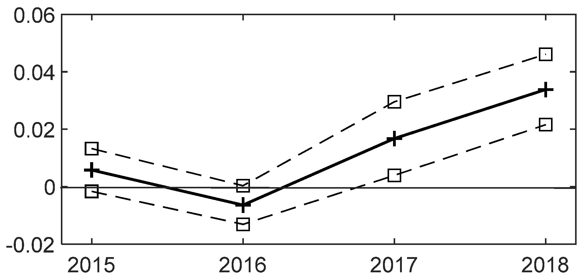
4.1. Parallel Trend Test and Correlation Test on DID

The DID method is based on the premise that there is no significant difference in the quality of innovation among firms in industries that are subject to different treatment sizes before the policy shock. Therefore, to test whether there is a significant difference in the quality of innovation among firms in different industries with economic entry barriers before and after the implementation of the negative list system for market access, this paper first conducts a parallel trend test, which is modeled as
Q u a l i t y i s j t = β 0 + t 2016 β t T r e a t s j t · D Y e a r t + γ X i s j t + u i + λ j + v s + τ t + ε i t ,
where Q u a l i t y i s j t denotes the innovation quality of firm i in industry j in region s at time t. D Y e a r t is a dummy variable indicating the year, and the other variables have the same meaning as in the baseline model. Coefficient β t , the coefficient of interest for the parallel trend test, indicates the difference in the quality of innovation of firms in industries with different economic entry barriers and thus deals with the intensity of the effect at time t of the year. If β t is significantly greater than 0, it indicates that the average innovation quality of firms in industries with stronger treatment effects at annual t is significantly higher than that of firms in industries with weaker treatment effects; conversely, if β t is statistically insignificant, it means that there is no significant difference in innovation quality between firms in industries with different treatment effects at annual t. The results of the parallel trend test using Equation (21) are reported in Table 1, where Column (1) does not include each control variable in the regression, while Column (2) takes into account the possible effects of each control variable on the regression results.
The results of the parallel trend test for DID in Table 1 show that the coefficient of Treat·D2015 is small, indicating that the differences in innovation quality among firms in different industries with economic entry barriers before the implementation of the negative list system for market access are small; meanwhile, the regression coefficient of Treat·D2015 is not statistically significant, indicating that after controlling for individual, industry, region and time fixed effects, the differences in the quality of innovation among firms in different industries with economic entry barriers in the pilot region are not significant in the year before the trial implementation of the negative list system for market access. Looking at the regression coefficients for the year after the implementation of the negative list system for market access, the coefficients of Treat·D2017 and Treat·D2018 are both significantly positive at least at the 5% level, indicating that the innovation quality of firms in industries with lower economic entry barriers in the pilot region is significantly higher than that of firms in industries with higher economic entry barriers in the two years after the pilot implementation of the negative list system for market access; furthermore, from the comparison of regression coefficients, the coefficient of Treat·D2017 is 2.87 times the regression coefficient of Treat·D2015, while the regression coefficient of Treat·D2018 is 2.02 times the coefficient of Treat·D2017, which indicates that the innovation quality of industries with lower economic entry barriers in the first year after the implementation of the negative list system for market access increased. In addition, there is a substantial increase in the effect after the implementation of the negative list system for market access as time progresses. The gap in the quality of innovation is increasing among firms in different industries that are treated differently by the policy. To visualize the differences in innovation quality among firms in different industries with economic entry barriers before and after the implementation of the negative list system for market access, this paper further draws a parallel trend graph based on the results of the parallel trend test, as shown in Figure 2. The solid line corresponds to the coefficient β t in Equation (21), while the area enclosed by the upper and lower dashed lines represents the 95% confidence interval of the regression coefficients; in addition, the coefficients of Treat·D2016 and their confidence intervals are obtained after taking 2015 as the base period and regressing again using Equation (21).
The parallel trend plot shows more intuitively that the regression coefficients vary near 0 before and in the year of the implementation of the negative list system for market access in 2016, and the 95% confidence intervals of the regression coefficients include 0. This indicates that there is no significant difference in the quality of innovation among firms in different industries with economic entry barriers before and in the year of the implementation of the negative list system for market access. The parallel trend plot also shows that the regression coefficients gradually increase in 2017–2018, after the implementation of the negative list system for market access, and none of the 95% confidence intervals of the regression coefficients include 0. This indicates that with the implementation of the negative list system for market access, there is a significant difference in the innovation quality of firms in different industries with economic entry barriers, and this difference tends to increase gradually. In summary, the results of the parallel trend test indicate that there is no significant difference in the quality of innovation of firms in different sectors of the treatment effect before the implementation of the negative list system for market access, so the setting of the DID specification is reliable.
We then proceed to conduct a correlation test between exogenous shock and variation in competition. The empirical study in this paper uses the implementation of the negative list system for market access as a natural experiment to examine the impact of competition on the quality of innovations. However, another basic premise for this analysis to hold is that the implementation of the negative list system for market access changes the level of competition in the market for nonprohibited and nonrestricted entry industries. Therefore, before examining the effect of competition on innovation quality using the DID method, it is necessary to test the correlation between the implementation of the negative list system for market access and changes in competition. The model to be tested is
C o m p s j t = β 0 + β 1 T r e a t t · I t P o s t + γ X i t + u i + λ j + v s + τ t + ε i t ,
where the explanatory variable C o m p s j t denotes the competition of industry j in region s at time t. Referring to Nickell [38] and Aghion [5], the competition of the industry is measured by the Lerner index, which is calculated as
C o m p s j t = 1 P r o f i t R e v i t ,
where P r o f i t denotes the total profit of firms in industry i in year t, and R e v i t is the main business income of firms in industry i. Intuitively, the Lerner index uses the amount of economic rent in an industry to measure its degree of competition, and its value is located in the interval of (0,1). Moreover, the Lerner index is proportional to the degree of competition, and the higher the intensity of competition is, the larger the Lerner index. If the Lerner index is equal to 1, it means that the profit of firms in the industry is 0 and the market is close to a perfectly competitive market. The Equation (23) coefficient β 1 , which is the coefficient of interest for the correlation test, represents the difference in competition between industries with different treatment effects before and after the implementation of the negative list system for market access, and if the estimation results show that β 1 is significantly greater than zero, it indicates that under the exogenous shock of the implementation of the negative list system for market access, the changes in the competition of industries with lower economic entry barriers are more significant and the degree of competition is significantly enhanced compared to industries with higher economic entry barriers.
The results of the correlation test between the implementation of the negative list system for market access and the changes in competition are reported in Columns (1) and (2) of Table 2. In particular, Column (1) of Table 2 does not include control variables, while Column (2) shows the regression results with the inclusion of each control variable. From the results of the correlation test between the implementation of the negative list system for market access and competition changes when no control variables are included in Column (1) of Table 2, it can be seen that the coefficient of T r e a t · I t P o s t is significantly positive at the 1% level, indicating that the increase in the level of competition in industries with lower economic entry barriers is significantly higher than the increase in the level of competition in industries with higher economic entry barriers after the implementation of the negative list system for market access; at the same time, the coefficient of T r e a t · I t P o s t indicates that, on average, the increase in competition in industries with lower economic entry barriers before and after the implementation of the negative list system for market access is 0.0049 higher than the increase in competition in industries with higher economic entry barriers. The results of the correlation test between the implementation of the negative list system for market access and changes in the level of competition after considering the effects of control variables in Column (2) of Table 2 show that the coefficient of T r e a t · I t P o s t is still significantly positive at the 1% level, indicating that the increase in the level of competition in industries with low economic entry barriers is significantly higher than the increase in the level of competition in industries with high economic entry barriers after the implementation of the negative list system for market access; at the same time, the regression coefficients of T r e a t · I t P o s t indicate that, on average, the increase in competition in industries with lower economic entry barriers before and after the implementation of the negative list system for market access is 0.0057 higher than the increase in competition in industries with higher economic entry barriers. The results of the correlation test between the implementation of the negative list system for market access and the changes in competition show that the implementation of the negative list system for market access leads to a change in the level of competition in nonprohibited and nonrestricted changes in the level of competition in industries, and the increase in the intensity of competition in industries with lower economic entry barriers is higher compared to industries with higher economic entry barriers. Therefore, the identification strategy of using the implementation of the negative list system for market access as a natural experiment to identify the impact of competition changes on innovation quality is feasible in this paper.

4.2. Baseline Estimates

Based on the parallel trend test and correlation test, we use the DID method to estimate the effect of competition on innovation quality. The regression results are reported in Columns (3) and (4) of Table 2. In particular, Column (3) of Table 2 is a bivariate regression excluding all control variables, while Column (4) shows the regression results with the inclusion of each control variable. From the baseline regression results in Column (3) of Table 2, it can be seen that the coefficient of T r e a t · I t P o s t is significantly positive at the 1% level, indicating that after the implementation of the negative list system for market access, the increase in the quality of firm innovation in industries with lower economic entry barriers and thus greater competition is significantly higher than the increase in the quality of innovation of firms in industries with smaller changes in competition, which implies that enhanced competition can more significantly improve the quality of firm innovation. Meanwhile, the regression coefficient of T r e a t · I t P o s t indicates that, on average, before and after the implementation of the negative list system for market access, the improvement in innovation quality of firms in industries with a greater increase in competition intensity is 0.0275 higher than the improvement in innovation quality of firms in industries with smaller changes in competition. The results of the baseline regression after considering the effects of control variables in Column (4) of Table 2 show that the coefficient of T r e a t · I t P o s t is still significantly positive at the 1% level, which indicates that enhanced competition can improve the quality of firm innovation relatively significantly. Meanwhile, the regression coefficient of T r e a t · I t P o s t shows that after considering the effect of control variables, on average, before and after the implementation of the negative list system for market access, the improvement in the quality of innovation of firms in industries with a greater increase in competition intensity is 0.0235 higher than the improvement in the quality of innovation of firms in industries with smaller changes in competition. The results of the combined benchmark regressions show that the implementation of the negative list system for market access improves the quality of innovation in nonprohibited and nonrestricted industries competition, and the improvement in the quality of innovation of firms in industries with lower economic entry barriers and thus higher competition is significantly higher compared to those with higher economic entry barriers and thus lower competition, suggesting that enhanced competition can significantly improve the quality of firm innovation.

4.3. Placebo Test

The results of the benchmark regressions suggest that the lower the economic entry barriers in the industry after the implementation of the negative list system for market access, the greater the increase in competition in the industry under the policy shock and the higher the quality of innovation of firms in the industry. However, the significant improvement in the quality of firms’ innovation may also be caused by reasons other than the implementation of the negative list system for market access. Therefore, to improve the robustness of the benchmark regression results, we further conduct a placebo test to verify whether the differences in firms’ innovation quality under different treatment effect strengths are caused by other shocks or random factors. The placebo test is conducted by imaging a fake policy implementation time and replacing the analyzed sample.
First, a placebo test is conducted using a fake policy implementation time method, where the year prior to the implementation of the negative list system for market access is used as a placebo to replace the year in which the treatment effect actually occurs, i.e., in the benchmark regression model when the year in which the sample data are located is 2015, I t P o s t is taken as 0, and conversely, when the year in which the sample data are located is 2016 or later years, I t P o s t is taken as 1. After the year of the fake policy implementation, the relationship between conducting competition and firm innovation quality is estimated using the econometric model shown in Equation (20), again using the DID method. If the regression results show that the coefficient β_1 is not significant, it indicates that there is no significant difference in innovation quality among firms in different industries with economic entry barriers before and after the dummy policy shock; therefore, the results of the benchmark regression are relatively robust. Conversely, if the coefficient β_1 is more significant, then it indicates that the differences in innovation quality of firms may be caused by other policy shocks or random factors. The results of the placebo test for virtual policy implementation time are shown in Columns (1) and (2) of Table 3. In particular, Column (1) does not include control variables, while Column (2) shows the regression results with the inclusion of each control variable.
As seen from the results of the correlation test between the implementation of the negative list system for market access and changes in competition when no control variables are included in Column (1) of Table 3, the coefficient of T r e a t · I t P o s t is not statistically significant, which indicates that there is no significant difference in the quality of innovation among firms in different sectors of the economic entry barriers after the time of placebo policy implementation. The results of the placebo test after considering the effect of control variables in Column (2) of Table 3 also show that the regression coefficients of T r e a t · I t P o s t are statistically insignificant, again indicating that there is no significant difference in the quality of innovation among firms in different industries with economic entry barriers after the virtual policy implementation time. Therefore, the results of the placebo test conducted at the time of the virtual policy indicate that the results of the benchmark regression are relatively robust.
Second, a placebo test is conducted using a replacement analysis sample, and the relationship between competition and the quality of innovation is estimated using the DID method shown in Equation (20) by reusing firms from regions in China that have not implemented the negative list system for market access as the analysis sample. If the regression results show that the coefficient β 1 is not significant, it indicates that there is no significant difference in the innovation quality of firms in regions without the implementation of the negative list system for market access before and after the policy implementation; conversely, if the coefficient β 1 is significant, it indicates that the differences in innovation quality of firms may be caused by other policy shocks or random factors. The results of the placebo test using the sample of firms in regions without negative market access lists are shown in Columns (3) and (4) of Table 3. In particular, Column (3) does not include control variables, while Column (4) shows the regression results with the inclusion of each control variable. From the results of the placebo test, none of the regression coefficients of T r e a t · I t P o s t are significant, which indicates that there is no significant difference in the innovation quality of firms in different economic entry barrier industries before and after the implementation of the negative list system for market access in regions where the negative list system for market access is not implemented. Therefore, the results of the placebo test using the replacement analysis sample approach indicate that the results of the benchmark regression in this paper are robust.

5. Discussion

This paper analyzes the impact of product competition on heterogeneous innovations from both theoretical and empirical perspectives. The first finding of our research is that competition has twofold impacts on the incentives of innovation. More competition implies a higher elasticity of substitution, leading to stronger incentives for innovation, while competition also decreases industry profits and increases the cost of innovation, which reduces the expected return on innovation, resulting in fewer incentives for innovation. When competition is low, the incentive effect of competition on innovation is more likely to dominate the inhibitory effect of competition; thus, more competition leads to more innovations. On the other hand, when the level of competition is above a certain threshold, the inhibitory effect of competition on innovation is dominant, and firms will not innovate due to low industry profits and rapidly rising R&D costs. Therefore, an inverted-U relationship exists between competition and innovation.
Most studies [5,39,40,41] on the relationship between competition and innovation have analyzed the inverted U-shaped relationship from the perspective of industry heterogeneity. For example, Aghion et al. [5] argued that competition tends to foster innovation in industries where firms operate at similar technological levels, while the Schumpeterian effect prevails in industries with large technological gaps; in contrast, Acemoglu and Akcigit [17] suggested that maintaining the technological gap in an industry provides stronger incentives for innovation. From a different perspective, this paper shows that competition may have both an incentive and an inhibitory effect on innovation regardless of the technological status of industries.
The second finding of this paper is that competition improves the allocation of innovation resources, which improves the quality of innovations. The reason is that a firm’s expected return on innovation is proportional to its innovation quality, leading to a higher exit threshold for high-quality firms compared to low-quality firms. Thus, as the level of competition increases, low-quality firms gradually withdraw from innovation, leaving more innovation resources to firms with high-quality innovations, and the overall innovation quality is improved.
The analysis of R&D subsidies by Acemoglu et al. [11] and Galaasen et al. [12] argued that although R&D subsidies increase aggregate R&D investment, they may have adverse growth and welfare implications by crowding out the R&D activity of high-efficiency innovators. This paper deepens the literature from the perspective of innovation quality. The findings of this paper suggest that competition can improve the allocation efficiency of innovation resources and reduce low-quality innovation. Therefore, although R&D subsidies can provide stronger incentives for innovation, they also raise the firm’s expected returns on innovation, which will lead low-quality firms that would have withdrawn from R&D investment at a certain level of competition to continue to innovate, resulting in misallocation of innovation resources and causing a decline in the overall innovation quality. Especially when the price elasticity of supply for innovation resources is relatively large, R&D subsidies will not cause a significant increase in the costs of innovations, leading to rapid growth of R&D investment, while the misallocation of innovation resources will worsen, resulting in a large number of low-quality innovations. In addition, the findings of this paper also indicate that R&D subsidies have a more significant impact on the decline of innovation quality of firms in low and medium-tech industries compared with high-tech industries. Since the constraints on innovation factor growth for low and medium-tech industries are weaker than those for high-tech industries, R&D subsidies lead to a higher increase in the expected profitability of innovation for firms in low- and medium-tech industries, leading to more serious distortions in the market, resulting in a more significant decline in the quality of innovation for firms in low- and medium-tech industries.

Author Contributions

Conceptualization, Z.Y. and X.W.; methodology, Z.Y. and X.W.; validation, X.W. and J.L.; investigation, X.W., J.L. and B.L.; writing—original draft preparation, X.W., J.L. and B.L.; writing—review and editing, J.L. and B.L.; supervision, Z.Y.; funding acquisition, Z.Y and J.L. All authors have read and agreed to the published version of the manuscript.

Funding

This research was funded by Beijing Municipal Government Advisory Committee decision consulting topic “Research on International Benchmarking and Ability Improvement of Beijing. Entrepreneurship-Incubation System”, grant number-Z201100009519011.

Data Availability Statement

Original data can be made available via [email protected].

Conflicts of Interest

The authors declare no conflict of interest. The funders had no role in the design of the study; in the collection, analyses, or interpretation of data; in the writing of the manuscript, or in the decision to publish the results.

Appendix A

In this section, we demonstrate the derivation of the demand function and the price elasticity of demand. The utility maximization problem for households is
max   q i 0 U = i = 1 n q i ε 1 ε ε ε 1 , s . t .   i = 1 n p i q i = m .
From the first-order condition for utility maximization, we can obtain
p i p j = q j q i 1 ε .
Taking ε − 1 powers on both sides of Equation (A2) yields
p i ε 1 j = 1 n p j 1 ε = q i 1 ε ε j = 1 n q j ε 1 ε .
We define the price index P and the product index Q as
P = i = 1 n p i 1 ε 1 1 ε , Q = i = 1 n q i ε 1 ε ε ε 1 .
Substituting the definitions of P and Q into Equation (A3), the first-order condition for the utility maximization problem can be expressed as
p i ε 1 P 1 ε = q i 1 ε ε Q ε 1 ε     p i P = q i Q 1 ε .
Solving for q i and p i , we can obtain the demand function q i p i , P , Q and the inverse demand function p i q i , P , Q as
q i = P ε Q p i ε , p i = P Q 1 / ε q i 1 / ε .
We now proceed to derive the price elasticity of demand. Substituting the inverse demand function in Equation (A6) into the budget constraint of the household, we can obtain
m = i = 1 n p i q i = i = 1 n q i ε 1 ε P Q 1 ε = Q ε 1 ε P Q 1 ε = P Q .
Substituting the budget constraint m = P Q into Equation (A6), the demand function for the product can be expressed as
q i = m p i ε P ε 1 .
From Equation (A8), the price elasticity of demand for product i can be obtained as
d q i d p i · p i q i = q i p i + q i P P p i p i q i = ε + 1 ε p i P 1 ε .
Equation (A9) shows that the price elasticity of demand for product i consists of two components. ε represents the direct effect of changes in the price of product i on its demand and 1 ε p i / P 1 ε represents the indirect effect of changes in the price index P due to a change in p i , and hence on the demand for product i. Supposing that p i = p j , the indirect effect of changes in the price of product i on its demand can be obtained from the definition of the market price index as
1 ε p i P 1 ε = 1 ε p i n p i 1 ε 1 1 ε 1 ε = 1 ε n .
Thus, as n + , 1 ε p i / P 1 ε 0 , which means that the indirect effect of changes in the price of product i on its demand is 0 when the number of products approaches infinity. Therefore, when there are a large number of products and the difference in product prices is relatively small, the indirect effect of changes in the price of product i on its demand can be treated as 0, and the price elasticity of demand for product i can be approximated as ε.

Appendix B

In this section, we derive the first-order condition for profit maximization. Since product i is supplied entirely by monopolistically competitive firm i, the demand function of firm i is given by Equation (A6). Thus, the profit function for firm i is π i = p i q i q i c i q i . The first-order condition for profit maximization is
d π i d q i = p i 1 + d p i d q i q i p i d c i d q i = 0 .
Substituting the marginal cost of firm i and the price elasticity of demand for product i into Equation (A11), the first-order condition for profit maximization can be expressed as
p i A i 1 1 ε = w .
Taking ε − 1 powers on both sides of Equation (A12), summing over i, and substituting the definitions of the price index P and the technology index A, the first-order condition for profit maximization can be expressed as
1 1 ε ε 1 A ε 1 = w ε 1 P 1 ε 1 1 ε A = w P .

Appendix C

In this section, we derive the firm’s profit in general equilibrium. The demand for product i in general equilibrium is equal to its supply. The demand function for product i is already given by Equation (A6), and since the supply of product i is q i = A i x i , the price of product i in general equilibrium satisfies
p i ε P ε Q = A i x i     p i = A i 1 ε x i 1 ε P Q 1 ε .
Substituting Equation (A14) into the first-order condition for profit maximization, we can obtain the relationship between firms’ inputs in general equilibrium as
x i x j = A i A j ε 1 .
Taking −1 powers on both sides of Equation (A15), summing over j, and substituting x i = X and the definition of the technology index A, we can rewrite Equation (A15) as
x i X = A i A ε 1 .
Substituting Equation (A16) into the firm’s production function q i = A i x i yields the supply of product i in general equilibrium as
q i = A i ε A 1 ε X .
Taking ε 1 / ε powers on both sides of Equation (A17), summing over i, and substituting the definitions of product index Q and technology index A gives
i q i ε 1 ε = A 1 ε ε 1 / ε X ε 1 ε i A i ε 1   Q = A X .
Substituting Equations (A17) and (A18) into Equation (A5) yields the price of the products in general equilibrium
p i = q i 1 ε Q 1 ε P = A i ε A 1 ε X 1 ε A X 1 ε P = A i 1 A P .
Equation (A19) also can be written as p i / P = A i / A 1 . It can be seen that the relative price of product i in general equilibrium is inversely proportional to the relative technological status of firm i. Thus, given that the technology of other firms remains unchanged, an improvement in the technology of firm i will lead to a decrease in the price of its product. Based on Equations (A19) and (A17), we can obtain the revenue of firm i in general equilibrium as
R i = p i q i = A i 1 A P · A i ε A 1 ε X = P A X A i A ε 1 .
Furthermore, from Equations (A13) and (A16), we can obtain the cost of firm i in general equilibrium as
c i = w x i = 1 1 ε P A A i ε 1 A 1 ε X = 1 1 ε P A X A i A ε 1 .
This gives the profit of firm i in general equilibrium as
π i = p i q i w x i = 1 ε A i ε 1 A 2 ε P X = 1 ε P A X A i A ε 1 ,
where A i / A ε 1 in Equation (A22) represents the relative technological status of firm i, and it can be easily seen that
A i A ε 1 = A i ε 1 j = 1 n A j ε 1     A i A ε 1 0 , 1 .
Adding up the profits of all firms and substituting the definition of A gives the total profits of firms in general equilibrium as
π = i = 1 n π i = 1 ε A 2 ε P X i = 1 n A i ε 1 = 1 ε P A X = 1 ε P Q .
By normalizing the price index at one, we can obtain firms’ profits in Equation (6).

Appendix D

In this section, we derive the Equations (7) and (8). The definition of A in Equation (4) is
A = i = 1 n A i ε 1 1 ε 1 ,
by which we can obtain
d A d A i = 1 ε 1 i = 1 n A i ε 1 1 ε 1 1 ε 1 A i ε 2 = i = 1 n A i ε 1 2 ε ε 1 A i ε 2 = A 2 ε A i ε 2 .
The profit of firm i in equilibrium is showed in Equation (6) where
π i = 1 ε A X A i A ε 1 = 1 ε A i ε 1 A 2 ε X .
Since A is a function of technological status of all firms π i is also a function of technological status of all firms. The differential of π i can be expressed as
d π i = π i A 1 d A 1 + π i A 2 d A 2 + π i A n d A n = π i A i d A i + j i π i A j d A j .
From Equation (A27), we can obtain
π i A i = ε 1 ε A i ε 2 A 2 ε X + 2 ε ε A i ε 1 A 1 ε X d A d A i .
Substituting Equation (A26) into Equation (A29), we can obtain
π i A i = ε 1 ε A i ε 2 A 2 ε X + 2 ε ε A i 2 ε 3 A 3 2 ε X .
By similar derivation we can obtain
π i A j = 2 ε ε A i ε 1 A 1 ε X d A d A j = 2 ε ε A i ε 1 A j ε 2 A 3 2 ε X .
Substituting Equations (A30) and (A31) into Equation (A28) we can obtain
d π i = ε 1 ε A i ε 2 A 2 ε X + 2 ε ε A i 2 ε 3 A 3 2 ε X d A i + j i 2 ε ε A i ε 1 A j ε 2 A 3 2 ε X d A j = π i ε 1 A i 1 + 2 ε A i ε 2 A 1 ε d A i + π i j i 2 ε A j ε 2 A 1 ε d A j = π i ε 1 + 2 ε A i A ε 1 d A i A i + π i j i 2 ε A j A ε 1 d A j A j ,
which is exactly Equation (7). η i represents firm’s technology elasticity of profit. Based on the definition of elasticities, η i can be expressed as
η i = π i A i A i π i .
Substituting Equation (A32) into Equation (A33), we can obtain
η i = π i A i A i π i = ε 1 ε A i ε 2 A 2 ε X + 2 ε ε A i 2 ε 3 A 3 2 ε X A i π i = 1 ε A i ε 1 A 2 ε X ε 1 A i 1 + 2 ε A i ε 2 A 1 ε A i π i = ε 1 + 2 ε A i A ε 1 = ε 1 ε 1 A i A ε 1 + A i A ε 1 = ε 1 1 A i A ε 1 + A i A ε 1 .
Denote A i A ε 1 by k i then we can obtain Equation (8).

Appendix E

In this section, we derive the price of innovation resources in equilibrium. The first-order condition for maximizing the expected return of innovation is
1 ρ 2 α π 0 δ i ε 1 + 2 ε n y i α 1 = ω .
Thus, the ratio of innovation resource demand between firm i and firm j with different innovation qualities can be expressed as
y i y j = δ i δ j 1 1 α .
The innovation quality index δ, which reflects the state of innovation quality of all firms, is defined as
δ = i = 1 n δ i 1 1 α 1 α .
In equilibrium, the total demand for innovation resource i = 1 n y i equals the total supply of innovation resource Y, i.e., i = 1 n y i = Y . Taking −1 powers on both sides of Equation (A26), summing over all firms, and substituting Equation (A27) and i = 1 n y i = Y into Equation (A26), we can rewrite the ratio of innovation resource input in equilibrium as
y i 1 j = 1 n y j = α i 1 1 β j = 1 n α j 1 1 β     y i Y = δ i δ 1 1 α .
Substituting Equation (A28) into Equation (A25), we can obtain the innovation resource price in equilibrium as
ω = 1 ρ 2 α π 0 δ ε 1 + 2 ε n Y α 1 .

References

  1. Schumpeter, J.A. Capitalism, Socialism and Democracy; Harper and Row: New York, NY, USA, 1942. [Google Scholar]
  2. Arrow, K.J. Economic Welfare and the Allocation of Resources for Invention; Princeton University Press: Princeton, NJ, USA, 1962; p. 609. [Google Scholar]
  3. Greenstein, S.; Ramey, G. Market structure, innovation and vertical product differentiation. Int. J. Ind. Organ. 1998, 16, 285–311. [Google Scholar] [CrossRef]
  4. Chen, Y.; Schwartz, M. Monopoly vs. Competition: Product innovation incentives. J. Econ. Manag. Strat. 2013, 22, 513–528. [Google Scholar] [CrossRef]
  5. Aghion, P.; Bloom, N.; Blundell, R.; Griffith, R.; Howitt, P. Competition and innovation: An inverted-U relationship. Q. J. Econ. 2005, 120, 701–728. [Google Scholar]
  6. Bloom, N.; Draca, M.; Van Reenen, J. Trade Induced Technical Change? The Impact of Chinese Imports on Innovation, IT and Productivity. Rev. Econ. Stud. 2016, 83, 87–117. [Google Scholar] [CrossRef] [Green Version]
  7. Campbell, D.L.; Mau, K. On “Trade induced technical change: The impact of Chinese imports on innovation, IT, and productivity”. Rev. Econ. Stud. 2021, 88, 2555–2559. [Google Scholar] [CrossRef]
  8. Autor, D.; Dorn, D.; Hanson, G.H.; Pisano, G.; Shu, P. Foreign Competition and Domestic Innovation: Evidence from U.S. Patents; Social Science Electronic Publishing: New York, NY, USA, 2017. [Google Scholar] [CrossRef]
  9. Hall, B.H.; Jaffe, A.; Trajtenberg, M. Market value and patent citations. Rand J. Econ. 2005, 36, 16–38. [Google Scholar]
  10. Akcigit, U.; Kerr, W.R. Growth through Heterogeneous Innovations. J. Politi-Econ. 2018, 126, 1374–1443. [Google Scholar] [CrossRef] [Green Version]
  11. Acemoglu, D.; Akcigit, U.; Alp, H.; Bloom, N.; Kerr, W. Innovation, reallocation, and growth. Am. Econ. Rev. 2018, 108, 3450–3491. [Google Scholar] [CrossRef] [Green Version]
  12. Galaasen, S.M.; Irarrazabal, A. R&D Heterogeneity and the Impact of R&D Subsidies. Econ. J. 2021, 131, 3338–3364. [Google Scholar] [CrossRef]
  13. Lentz, R.; Mortensen, D.T. An Empirical Model of Growth Through Product Innovation. Econometrica 2008, 76, 1317–1373. [Google Scholar] [CrossRef]
  14. Raith, M. Competition, risk, and managerial incentives. Am. Econ. Rev. 2003, 93, 1425–1436. [Google Scholar] [CrossRef]
  15. Bauner, C. Mechanism choice and the buy-it-now auction: A structural model of competing buyers and sellers. Int. J. Ind. Organ. 2015, 38, 19–31. [Google Scholar] [CrossRef]
  16. Liu, T.X. All-pay auctions with endogenous bid timing: An experimental study. Int. J. Game Theory 2018, 47, 247–271. [Google Scholar] [CrossRef]
  17. Juang, W.-T.; Sun, G.-Z.; Yuan, K.-C. A model of parallel contests. Int. J. Game Theory 2020, 49, 651–672. [Google Scholar] [CrossRef]
  18. Da Silveira, B.S.; De Mello, J.M.P. Campaign Advertising and Election Outcomes: Quasi-natural Experiment Evidence from Gubernatorial Elections in Brazil. Rev. Econ. Stud. 2011, 78, 590–612. [Google Scholar] [CrossRef] [Green Version]
  19. Chu, Y. Optimal capital structure, bargaining, and the supplier market structure. J. Financ. Econ. 2012, 106, 411–426. [Google Scholar] [CrossRef]
  20. Acemoglu, D.; Gancia, G.; Zilibotti, F. Competing engines of growth: Innovation and standardization. J. Econ. Theory 2012, 147, 570–601. [Google Scholar] [CrossRef]
  21. Deng, S.; Li, B.; Wu, K. Analysing the impact of high-tech industry on regional competitiveness with principal component analysis method based on the new development concept. Kybernetes 2022. [Google Scholar] [CrossRef]
  22. Nidumolu, R.; Prahalad, C.K.; Rangaswami, M.R. Why sustainability is now the key driver of innovation. Harvard Bus. Rev. 2009, 87, 56. [Google Scholar]
  23. Yao, M.; Di, H.; Zheng, X.; Xu, X. Impact of payment technology innovations on the traditional financial industry: A focus on China. Technol. Forecast. Soc. Chang. 2018, 135, 199–207. [Google Scholar] [CrossRef]
  24. Wei, T.; Zhu, Z.; Li, Y.; Yao, N. The evolution of competition in innovation resource: A theoretical study based on Lotka–Volterra model. Technol. Anal. Strat. Manag. 2018, 30, 295–310. [Google Scholar] [CrossRef]
  25. Heywood, J.S.; Wang, Z.; Ye, G. R&D rivalry with endogenous compatibility. Manch. Sch. 2022, 90, 354–384. [Google Scholar] [CrossRef]
  26. Braga, J.P.; Semmler, W.; Grass, D. De-risking of green investments through a green bond market–Empirics and a dynamic model. J. Econ. Dyn. Control 2021, 131, 104201. [Google Scholar] [CrossRef]
  27. Cozzolino, A.; Rothaermel, F.T. Discontinuities, competition, and cooperation: Coopetitive dynamics between incumbents and entrants. Strat. Manag. J. 2018, 39, 3053–3085. [Google Scholar] [CrossRef]
  28. Nunn, N.; Qian, N. The potato’s contribution to population and urbanization: Evidence from a historical experiment. Q. J. Econ. 2011, 126, 593–650. [Google Scholar] [CrossRef]
  29. Grimm, M.; Krüger, J.; Lay, J. Barriers to entry and returns to capital in informal activities: Evidence from sub-saharan africa. Rev. Income Wealth 2011, 57, S27–S53. [Google Scholar] [CrossRef] [Green Version]
  30. Lofstrom, M.; Bates, T.; Parker, S.C. Why are some people more likely to become small-businesses owners than others: Entrepreneurship entry and industry-specific barriers. J. Bus. Ventur. 2014, 29, 232–251. [Google Scholar] [CrossRef]
  31. Couto, A.; Barbosa, N. Barriers to entry: An empirical assessment of Portuguese firms’ perceptions. Eur. Res. Manag. Bus. Econ. 2020, 26, 55–62. [Google Scholar] [CrossRef]
  32. Kudová, D.; Chládková, H. Barriers to the entry into the fruit producing industry in the Czech Republic. Agric. Econ.–Czech 2008, 54, 413–418. [Google Scholar] [CrossRef] [Green Version]
  33. Jensen, C. Competition as an engine of economic growth with producer heterogeneity. Macroecon. Dyn. 2016, 20, 362–379. [Google Scholar] [CrossRef]
  34. Kim, N.; Min, S. Impact of Industry Incumbency and Product Newness on Pioneer Leadtime. J. Manag. 2012, 38, 695–718. [Google Scholar] [CrossRef]
  35. Gil, R.; Ruzzier, C.A. The Impact of Competition on “Make-or-Buy” Decisions: Evidence from the Spanish Local TV Industry. Manag. Sci. 2018, 64, 1121–1135. [Google Scholar] [CrossRef] [Green Version]
  36. Yu, L.; Dai, H.; Cai, S. A research on the influence effect of innovation quantity and innovation quality on foreign trade export. Sci. Res. Manag. 2019, 40, 116–125. [Google Scholar]
  37. Jin, P.; Yin, D.; Jin, Z. Urban heterogeneity, institution supply and innovation quality. J. World Econ. 2019, 42, 99–123. [Google Scholar]
  38. Nickell, S.J. Competition and Corporate Performance. J. Politi-Econ. 1996, 104, 724–746. [Google Scholar] [CrossRef]
  39. Acemoglu, D.; Aghion, P.; Zilibotti, F. Distance to frontier, selection, and economic growth. J. Eur. Econ. Assoc. 2006, 4, 37–74. [Google Scholar] [CrossRef]
  40. Griffith, R.; Redding, S.; Simpson, H. Technological catch-up and geographic proximity. J. Reg. Sci. 2009, 49, 689–720. [Google Scholar] [CrossRef]
  41. Negassi, S.; Lhuillery, S.; Sattin, J.-F.; Hung, T.-Y.; Pratlong, F. Does the relationship between innovation and competition vary across industries? Comparison of public and private research enterprises. Econ. Innov. New Technol. 2019, 28, 465–482. [Google Scholar] [CrossRef]
Figure 1. Thresholds of Competition for Firms to Exit.
Sustainability 14 07562 g001
Figure 2. Parallel trend diagram of DID (The solid line indicates the regression coefficients, and the dashed line indicates the 95% confidence intervals of the regression coefficients).
Sustainability 14 07562 g002
Table 1. Parallel trend test for DID.
Variable(1)(2)
Treat·D20150.00410.0058
(0.0035)(0.0038)
Treat·D20170.0209 ***0.0167 **
(0.0058)(0.0065)
Treat·D20180.0360 ***0.0338 ***
(0.0059)(0.0063)
Control variablesNoYes
Individual fixed effectsYesYes
Industry fixed effectsYesYes
Regional fixed effectsYesYes
Year fixed effectsYesYes
R 2 0.44170.4731
Note: ** Significant at the 5% level; *** Significant at the 1% level.
Table 2. Correlation test and DID regression results.
VariableComp
(1)
Comp
(2)
Quality
(3)
Quality
(4)
T r e a t · I t P o s t 0.0049 ***0.0057 ***0.0275 ***0.0235 ***
(0.0016)(0.0017)(0.0050)(0.0056)
RD 0.0000 0.0000
(0.0000) (0.0000)
RDL 0.0005 0.0070 ***
(0.0004) (0.0020)
techBase −0.0001 ** 0.0050 ***
(0.0000) (0.0007)
ROS 0.0000 −0.0001 **
(0.0000) (0.0001)
Age −0.0102 −0.0423
(0.0128) (0.0739)
Individual fixed effectsYesYesYesYes
Industry fixed effectsYesYesYesYes
Regional fixed effectsYesYesYesYes
Year fixed effectsYesYesYesYes
R 2 0.56600.57890.44160.4729
Note: ** Significant at the 5% level; *** Significant at the 1% level.
Table 3. Placebo test for DID.
Variable(1)(2)(3)(4)
T r e a t · I t P o s t *0.00330.0026−0.0037−0.0067
(0.0033)(0.0035)(0.0037)(0.0041)
RD 0.0000 0.0000
(0.0000) (0.0000)
Researcher 0.0070 *** 0.0101 ***
(0.0022) (0.0024)
techBase 0.0049 *** 0.0023 *
(0.0008) (0.0014)
ROS −0.0001 * 0.0000
(0.0000) (0.0000)
Age −0.0572 0.0266
(0.0966) (0.0222)
Individual fixed effectsYesYesYesYes
Industry fixed effectsYesYesYesYes
Regional fixed effectsYesYesYesYes
Year fixed effectsYesYesYesYes
R 2 0.45810.48610.46680.4906
Note: * Significant at the 10% level; *** Significant at the 1% level.
Publisher’s Note: MDPI stays neutral with regard to jurisdictional claims in published maps and institutional affiliations.

