Quantifying Raveling Using 3D Technology with Loss of Aggregates as a New Performance Indicator

Abstract

Pavement raveling is one of the predominant distresses in the United States that impacts roadway safety and driver comfort on open-graded friction course (OGFC) pavements. Raveling specific treatments, such as fog seal and micro-milling the OGFC layer, can prolong pavement life and reduce resurfacing costs and environmental impact. However, with the current qualitative condition assessment methods (which rate pavements at Severity Levels 1–3 or as light, moderate, or severe), it is difficult to determine the optimal timing for these raveling treatments to be most effective. Therefore, there is an urgent need to develop a method to quantitatively evaluate the raveling condition. While 3D pavement technology provides opportunities for quantifying pavement raveling conditions using 3D pavement surface data, there are two main challenges for quantifying pavement raveling: (1) estimating a reference surface that represents the pavement without any raveling so that the actual pavement can be compared to the reference surface to quantify the raveling, and (2) obtaining pavement images with quantified raveling conditions (aggregate loss volume) for validation. This paper proposes a method with the loss of aggregate as a new performance indicator to automatically quantify raveling using 3D pavement surface data already collected by transportation agencies for pavement evaluation. The proposed method is validated using pavement images (with known aggregate loss) from simulated pavement mats fabricated in the lab and synthetic pavement images obtained by procedural generation. The proposed method consists of (1) 3D data acquisition; (2) pre-processing with (a) outlier removal and image smoothing, (b) two-sensor image stitching, and (c) range image rectification; (3) raveling detection using (a) region of interest selection, (b) reference surface estimation, (c) potential aggregate loss identification, and (d) noise removal; and (4) aggregate loss quantification. The validation results show a strong correlation (R = 0.99) between the computed aggregate loss and the expected aggregate loss. Better performance was observed with the proposed method than with other methods (such as the watershed method and the model fitting method). The proposed method provides a cost-effective means to quantify the loss of aggregates in support of quantitative raveling condition forecasting by leveraging 3D pavement data already collected by transportation agencies.

1. Introduction

Pavement raveling is one of the leading causes of failure of porous pavement, such as open-graded friction course (OGFC), since the porous nature of the pavement means smaller contact areas among the aggregates. OGFC is widely used in the southern states [1], such as Georgia, to reduce water spray and hydroplaning during rainy conditions. For example, OGFC is used on the entire interstate asphalt pavement system in the state of Georgia. Since raveling is one of the predominant pavement distresses affecting OGCF pavements, monitoring raveling conditions and applying appropriate treatments at the optimal timing to prolong the pavement surface life span is an important problem to address. The current raveling survey method generally categorizes the raveling severity into three levels, such as those used by the Georgia Department of Transportation (GDOT), which classifies raveling by Severity Levels 1–3 [2]. Similarly, the Florida Department of Transportation (FDOT), Oregon Department of Transportation (ODOT), and Texas Department of Transportation (TxDOT) use severity levels of light, moderate, and severe [3,4,5]. These classification methods only provide a qualitative measure of the raveling condition and might be subjective from rater to rater. Using these survey methods, raveling conditions can stay at the same severity level for many years before moving to the next level, making the forecast of raveling using these measurements a difficult task to perform. The current raveling rating system lacks granularity to differentiate different percentages of loss aggregate (raveling), which is important for making adequate decisions on determining the right pavement preservation methods, such as fog seal (to prolong the pavement long) and micro-milling and thin overlay [6,7]. Based on a previous study, fog seal was shown to be most effective for certain percentages of loss aggregates at Severity Level 1 [8]. However, the current qualitative severity levels are unable to provide the required granularity to maximize the effectiveness of fog seal. In addition, the qualitative measurement is also difficult to support forecasting. Therefore, there is an urgent need to develop a quantitative raveling condition measurement method to support the determination of the right treatment and the most effective condition forecasting.

The advancements in 3D pavement technology provide a great opportunity to quantitively assess raveling using the percentage of aggregate loss. In a survey reported in 2017, thirty-five states indicated they were using a 3D automated data collection system or planned to use such a system within the next two years [9]. In many states, high-resolution 3D pavement range images have been collected for pavement evaluation for many years. The method proposed in this paper can be used to quantify raveling conditions with the 3D pavement data, which is already collected by all 50 states; it can be used to determine adequate pavement preservation, such as fog seal, to prolong pavement life. This has not previously been possible to achieve. The developed quantitative measure and technology method could be impactful nationwide and worldwide because of its ability to maximize pavement preservation effectiveness.

Three-dimensional (3D) pavement surface data have been used to automatically and semi-automatically extract pavement distresses; they have been used in many pavement studies, including the following: detecting and measuring cracking [10,11] and its deterioration [12], rutting [13,14], concrete joint faulting [15], project-level micro-milling pavement surface texture construction quality control [16], automatic pothole detection [17], and a new area-based faulting measurement with enhanced accuracy [18]. However, there are only a limited number of studies that have used 3D pavement data to quantitatively measure the pavement raveling condition.

Previous studies have used the standard deviation of a range of an image’s pixel values as an indicator to classify raveling conditions [19] or a range value to determine the volume of surface material loss [20]. While a standard deviation is a good indicator of surface roughness, it cannot be used to physically quantify aggregate loss due to raveling. For methods that quantify raveling through the determination of aggregate loss volume, it is important to determine the accurate reference surface for quantifying aggregate loss. A reference surface represents the pavement surface in its pristine conditions, that is, with no aggregate loss. However, there are technical challenges in that reference surface estimation becomes more difficult with more aggregate loss, and this leads to results that generally underestimate the aggregate loss of more severe raveling conditions. Therefore, there is a need to develop an enhanced approach to quantify pavement aggregate loss.

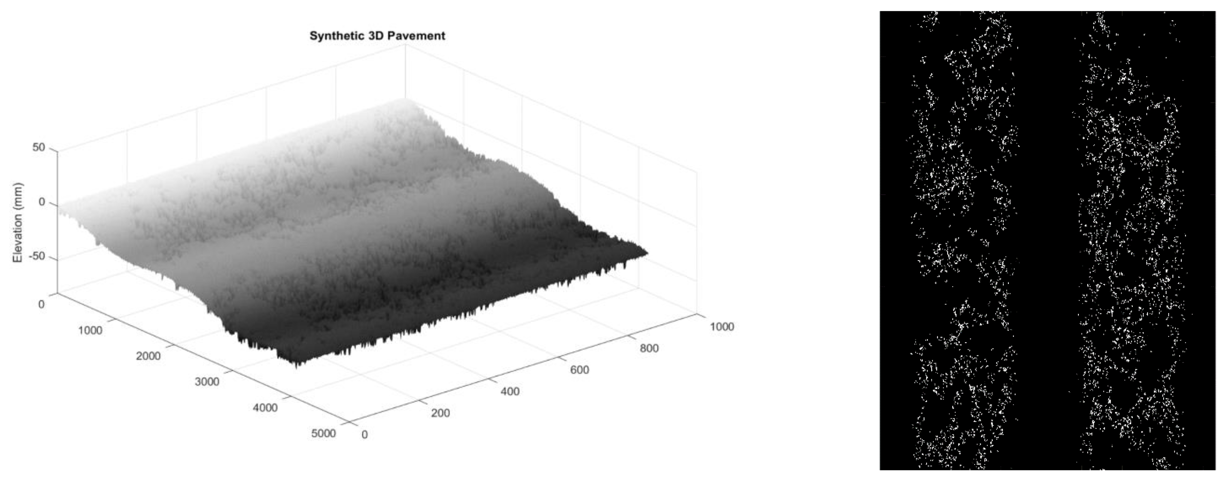
Additionally, previous attempts to quantify aggregate loss have also lacked a systematic validation process to comprehensively evaluate the performance of the proposed methods. To validate any method that aims to quantify the loss of aggregate on a pavement surface, true aggregate loss references need to be established; in other words, the amount of aggregate loss on a pavement surface needs to be measured. Such a task is very difficult to perform on real-world pavement surfaces; therefore, a procedure that can produce pavement surfaces or range images with known aggregate loss values is required to validate the proposed method.

The focus of this paper is to propose a method to quantify raveling conditions, and the objectives of this paper are the following: (1) to develop a method to quantify raveling conditions with the loss of aggregate with a new performance indicator using 3D pavement surface images data already collected, (2) to develop a fabricated pavement mat and procedurally generate synthetic pavement images with the known loss of aggregate values, and (3) to critically validate the accuracy of the proposed method.

The paper is organized as follows. First, the background and objective of this paper are presented. Second, the proposed method and its steps are presented. Third, the validation procedure of the proposed method is shown. Fourth, the performance of the proposed method is compared to other methods that can quantify material loss on a surface. Finally, conclusions and recommendations are made.

2. Proposed Method

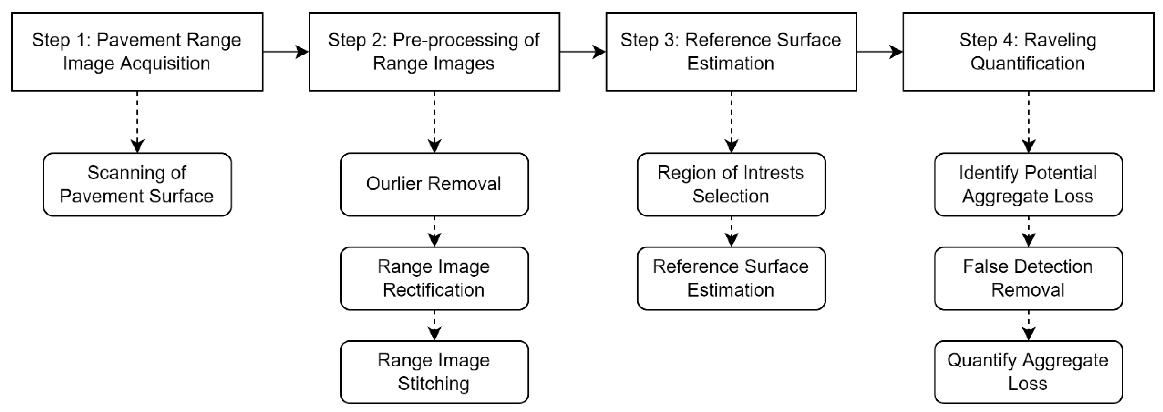
To perform automatic raveling detection and quantification using 3D pavement range images and the loss of aggregate as a new performance indicator, a method is proposed. The proposed method, at its core, first estimates a reference surface that represents the pavement in its pristine condition with no aggregate loss. Then, based on the reference surface, the proposed method identifies and quantifies material loss on a pavement surface. As presented in Figure 1, the proposed method uses the following steps: (1) pavement range data acquisition, (2) pre-processing of the pavement range image, (3) reference surface estimation, and (4) raveling quantification.

2.1. Step 1: Pavement Range Data Acquisition

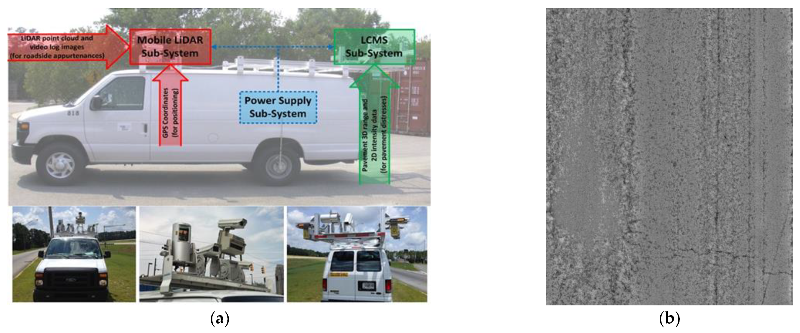
In this study, the Georgia Tech Sensing Vehicle (GTSV), equipped with a 3D pavement laser system, was used to collect the pavement range images. The GTSV, as shown in Figure 2a, was sponsored by the US DOT and GDOT. It consists of a pair of high-frequency pavement profiling lasers (LCMS, manufactured by INO/Pavemetrics) that can operate up to 5.6 kHz at highway speed (60 mph). The detailed pavement range images obtained from the laser system have a longitudinal resolution of 5mm, a transverse resolution of 1 mm, and a 0.5 mm resolution of elevation measurement at each data point. The pavement range images were used to estimate the reference surface, and then identify and quantify the aggregate loss. Figure 2b shows an example of a pavement range image with raveling at Severity Level 3.

2.2. Step 2: Pre-Processing Pavement Range Images

The goal of pre-processing is to prepare the acquired range images for raveling detection in later steps. Pre-processing involves three sub-steps (detailed in this section) to remove noise from the range image, rectify the range image to remove cross slope and other pavement deformations (such as rutting), and, finally, to stitch together the range images from two laser sensors to establish a full-lane range image.

2.2.1. Step 2.1: Remove Noise and Smooth Range Image Using Gaussian Filter

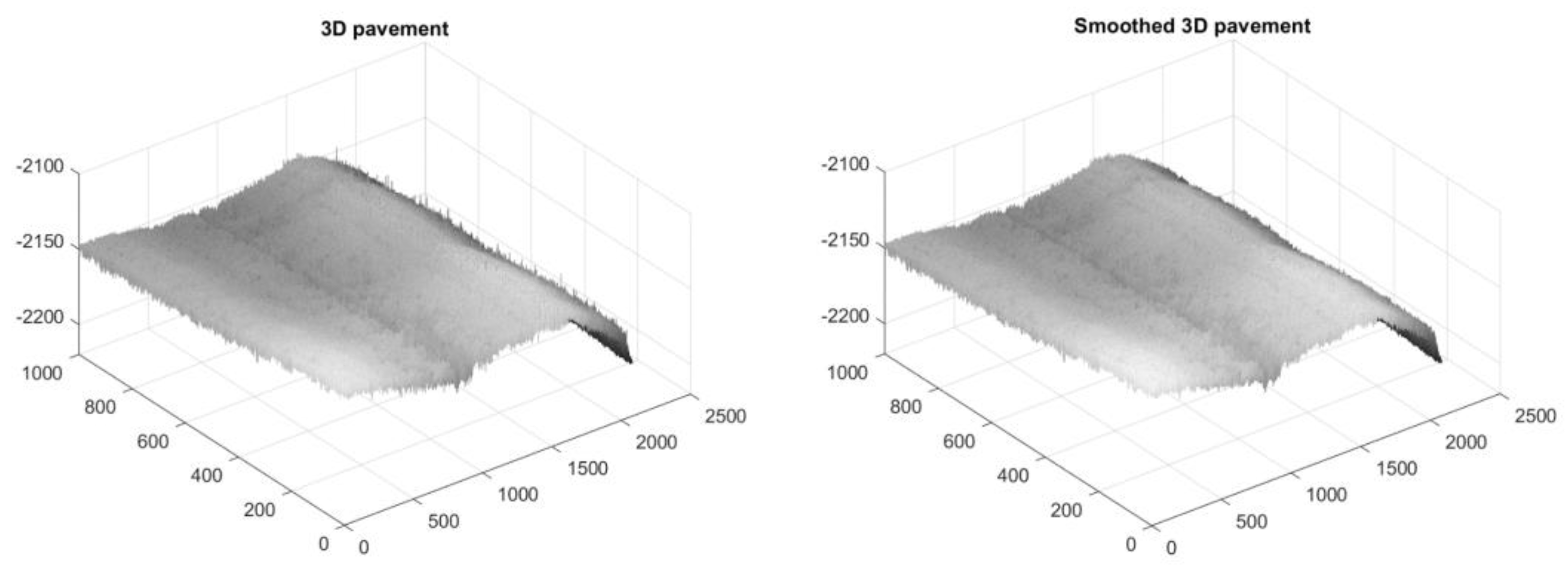
The obtained raw range image can contain some missing data points and noisy data points caused by the 3D laser device and surface conditions (e.g., shiny surfaces, wet surfaces). To mitigate the effect of the noise on raveling detection, missing data points on the surface are first filled using linear interpolation, and then the surface data is smoothed using a Gaussian filter. Figure 3 shows an example of a 3D pavement surface being processed to remove spikes (noises).

2.2.2. Step 2.2: Rectify (Level) Range Image Surface by Removing Cross Slope and Rutting

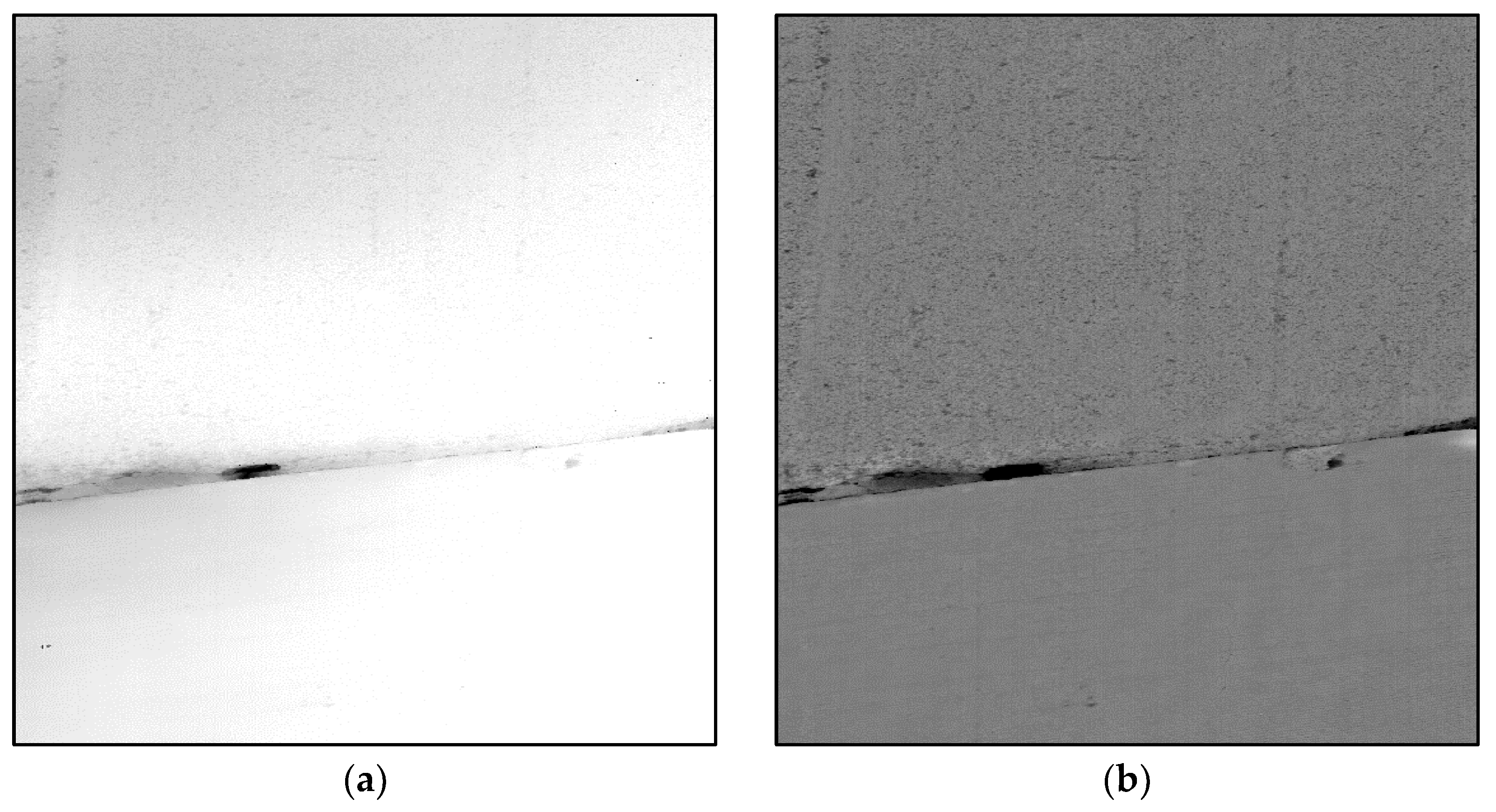
As shown in the Figure 3, the collected 3D pavement is not a flat surface but a complex shape that consists of varying pavement features, such as cross slope and edge drop-off, and pavement deformations, such as rutting. To rectify a range image is to remove these macro-features so that localized features, such as cracks, joints, and aggregate loss, can be enhanced and more easily identified. Figure 4a shows an example of a range image before rectification. After rectification, the joint and material loss on the pavement is easier to see, as shown in the rectified image in Figure 4b. The rectification can be performed using a moving average filter.

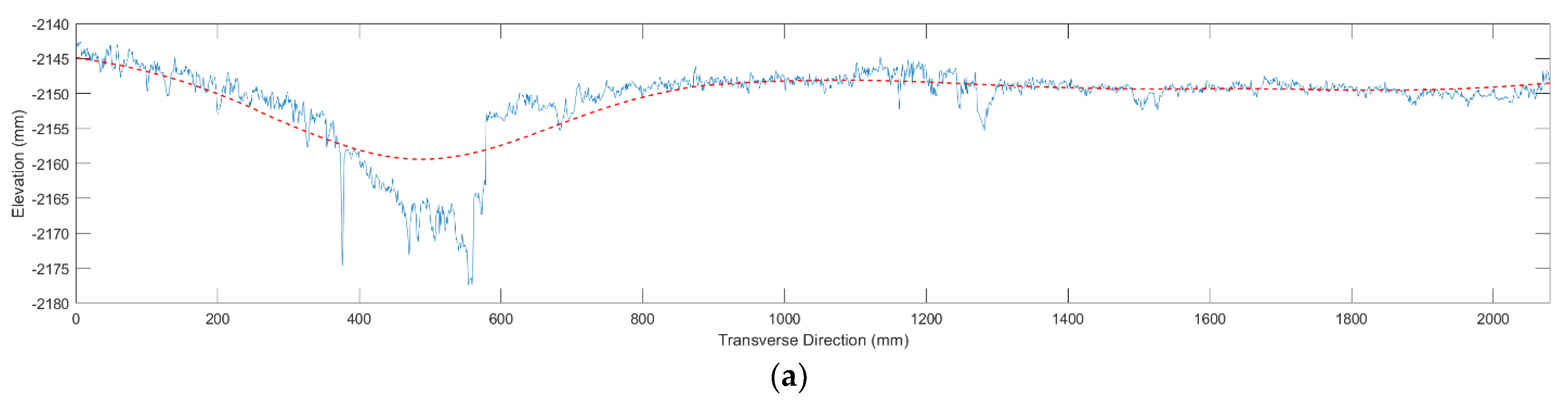
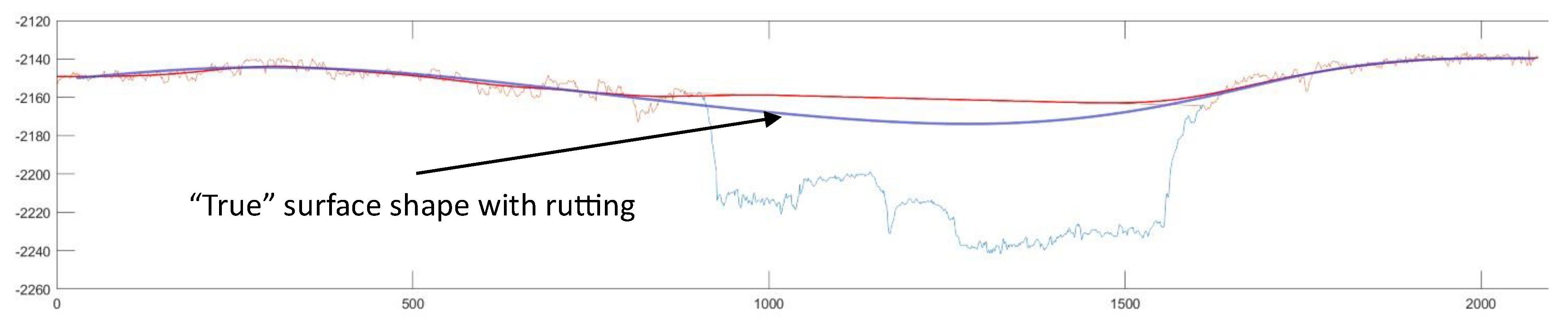
Rectification can be performed using the moving average of each transverse profile to extract the general shape of the pavement. Then, the values from the moving average profiles are subtracted from each corresponding transverse profile to obtain the rectified profiles. However, if the transverse profile contains areas that have large elevation drops over a wide area, as the length of the area approaches the moving average window size, the rectified image can no longer preserve the amount of elevation change visible on the original range image, Figure 5a shows how the moving average (red line) would “dip” at a location with high material loss. Since the objective of the proposed method is to quantify both the aggregate loss area and aggregate loss volume, not being able to preserve the elevation change will cause an underestimation of the aggregate. Therefore, areas with “wide raveling” need to be identified and treated differently in rectification. 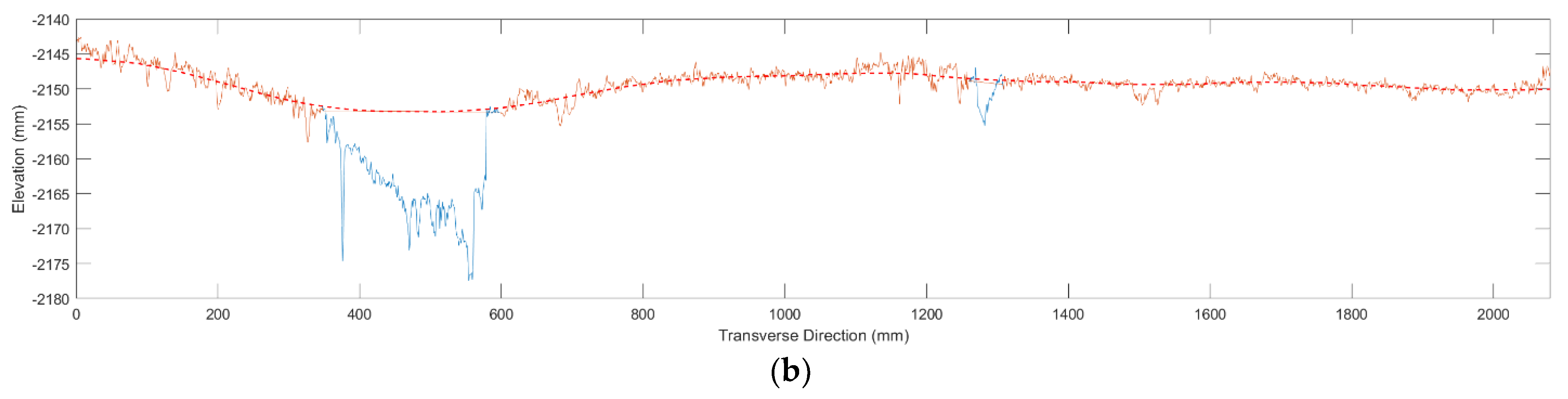Figure 5b shows rectification with wide-raveling identification; the moving average (red dashed line) captured the general shape of the pavement without a “dip” at the location with high material loss. The moving average algorithm used in this figure has a window size of 20, which is 20 mm in real-world distance.

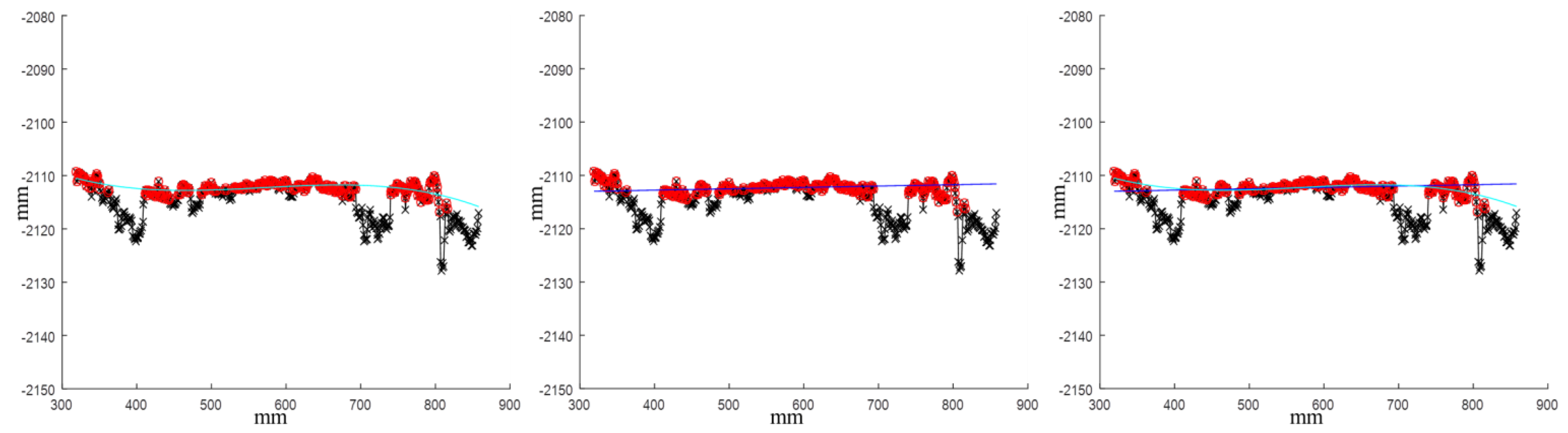
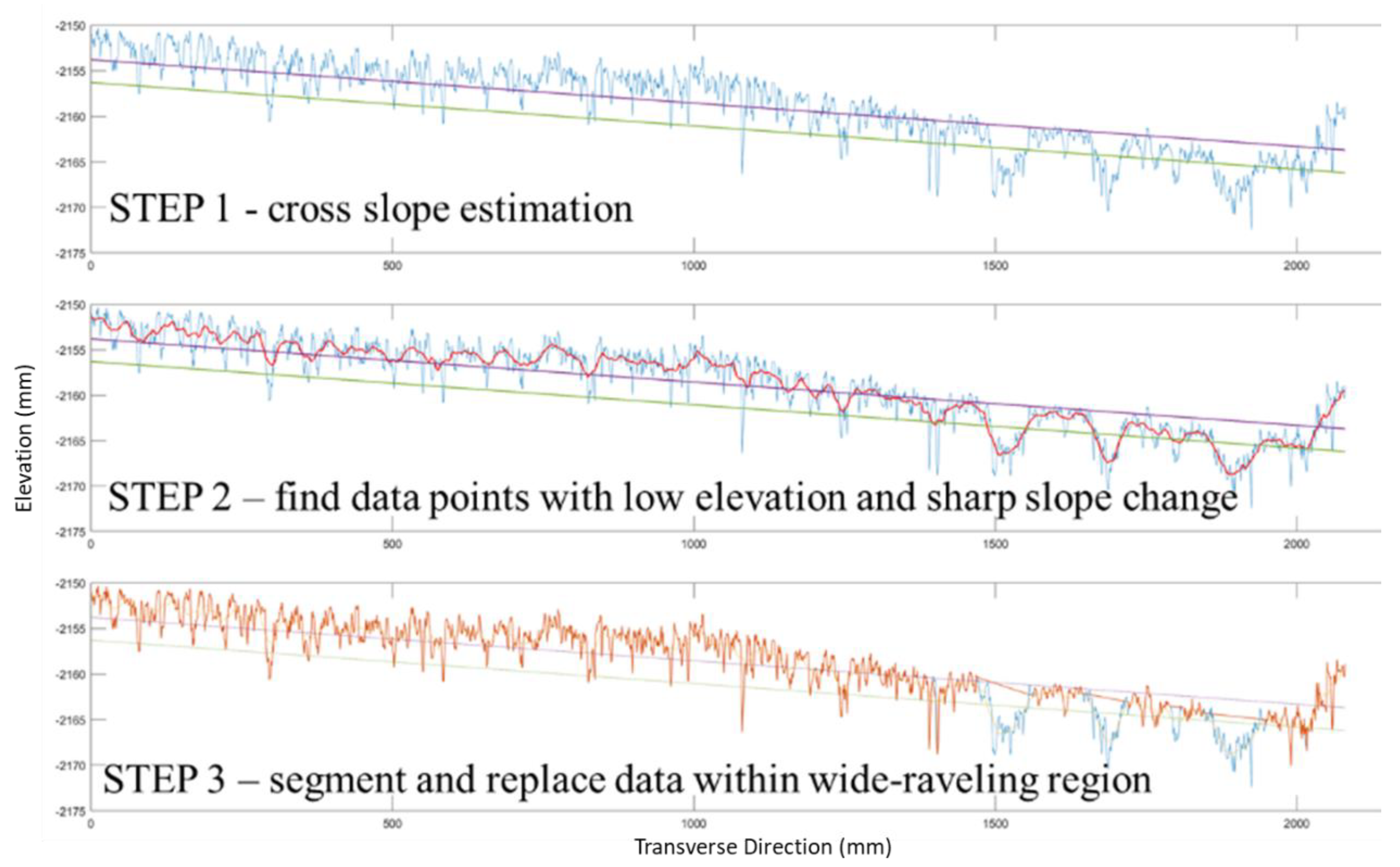
Figure 6 shows how wide-raveling identification is performed. First, the cross slope is estimated by fitting the transverse profile (blue line) with a first-order polynomial (purple line). Second, the moving average with a small window size (window size = 20) is used to smooth out the transverse profile (red line). Then, areas with low elevation, defined as a lower threshold than the fitted first-order polynomial (green line) and also accompanied by a sharp elevation change (defined based on the profile slope) are segmented and labeled as a wide-raveling area. During rectification using a moving average, to avoid using data from the wide-raveling area, data points within each wide-raveling area are replaced by a linear interpolation between the beginning and end of each wide-raveling area, as shown in Figure 6 Step 3.

2.2.3. Step 2.3: Stitch Two-Sensor Images to Establish Full-Lane Pavement Range Image

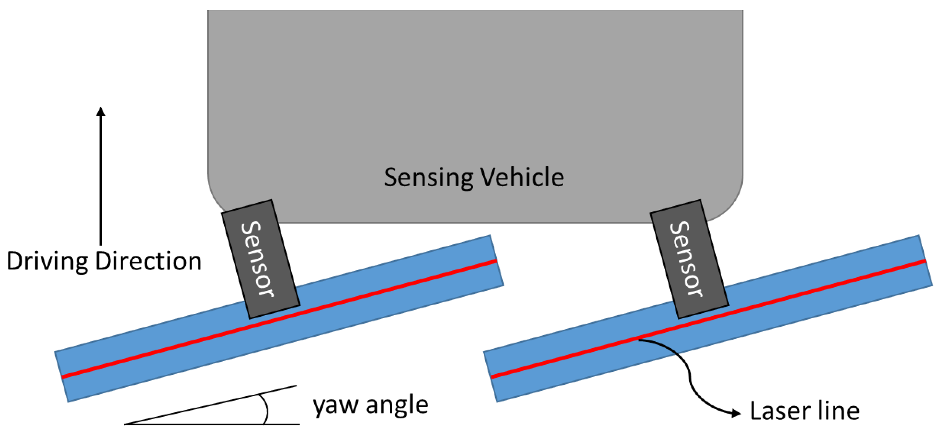
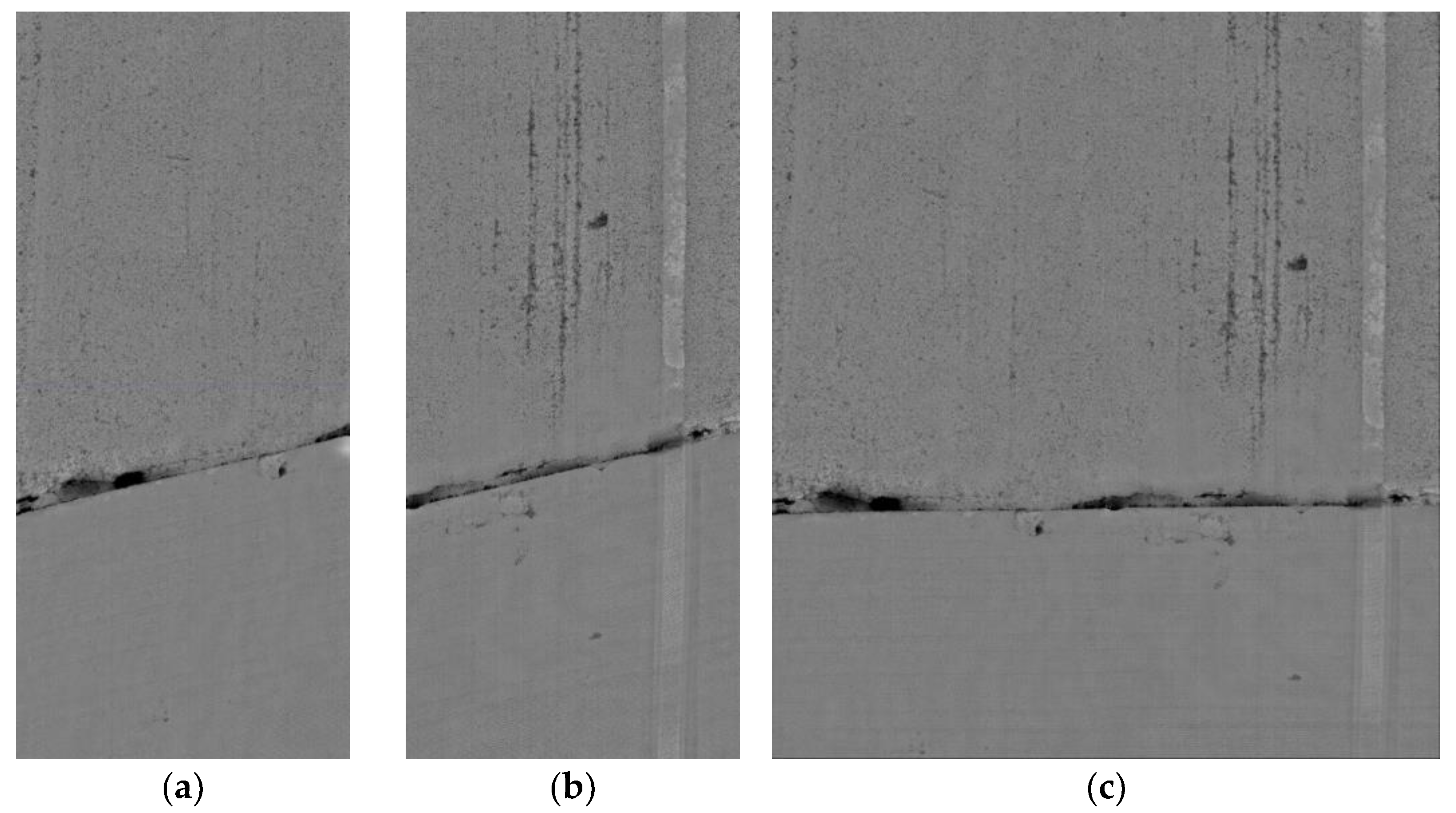
The laser system equipped on the GTSV uses two 3D laser sensors to collect pavement range data. Because the sensors are set up to have a small angle between the line laser and the transverse direction of the road to avoid the laser from one sensor interfering with the other sensor, as shown in Figure 7, the range image collected is skewed from its actual orientation. In Figure 8a,b range images collected by the laser sensors on the GTSV are shown; each image covers roughly half the width of the traveled lane. The pavement joints on these images are actually in the transverse direction of the road, but because of the angle of the sensor, the pavement joints in the images are skewed. Therefore, after rectification, the range images are rotated and stitched to form a full-lane pavement image, as shown in Figure 8c.

2.3. Step 3: Reference Surface Estimation

Using the range images prepared in pre-processing, loss of aggregate is detected using the four processing steps detailed in this section. The outcome from this step is a binary image indicating the location of the detected aggregate loss on the pavement surface.

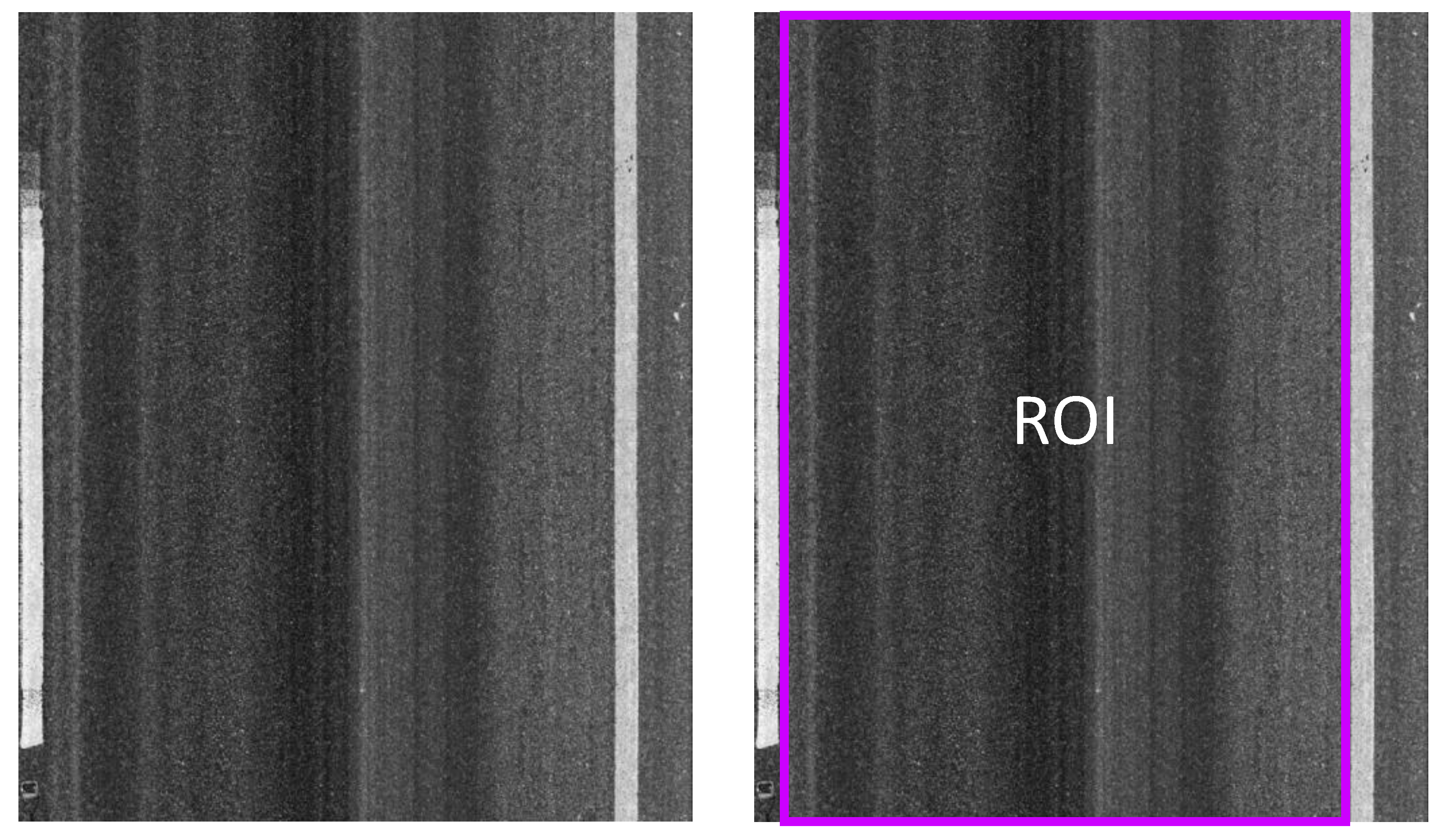
2.3.1. Step 3.1: Using Pavement Markings to Select Regions of Interest (ROIs)

The 3D laser system used in this study collects range images and intensity images of the pavement. From the intensity images, highly reflective surfaces, such as pavement markings, can be easily identified, as shown in Figure 9. By selecting the ROI for the detected loss of aggregate within the lane marking, this process effectively removes other features, such as pavement markings, road reflectors, rumble strips, and cold joints at the edge of pavements, which may be captured by the laser sensors. Removing these features reduces noise and makes the pavement within the ROI more predictable, thus improving the performance of the proposed method.

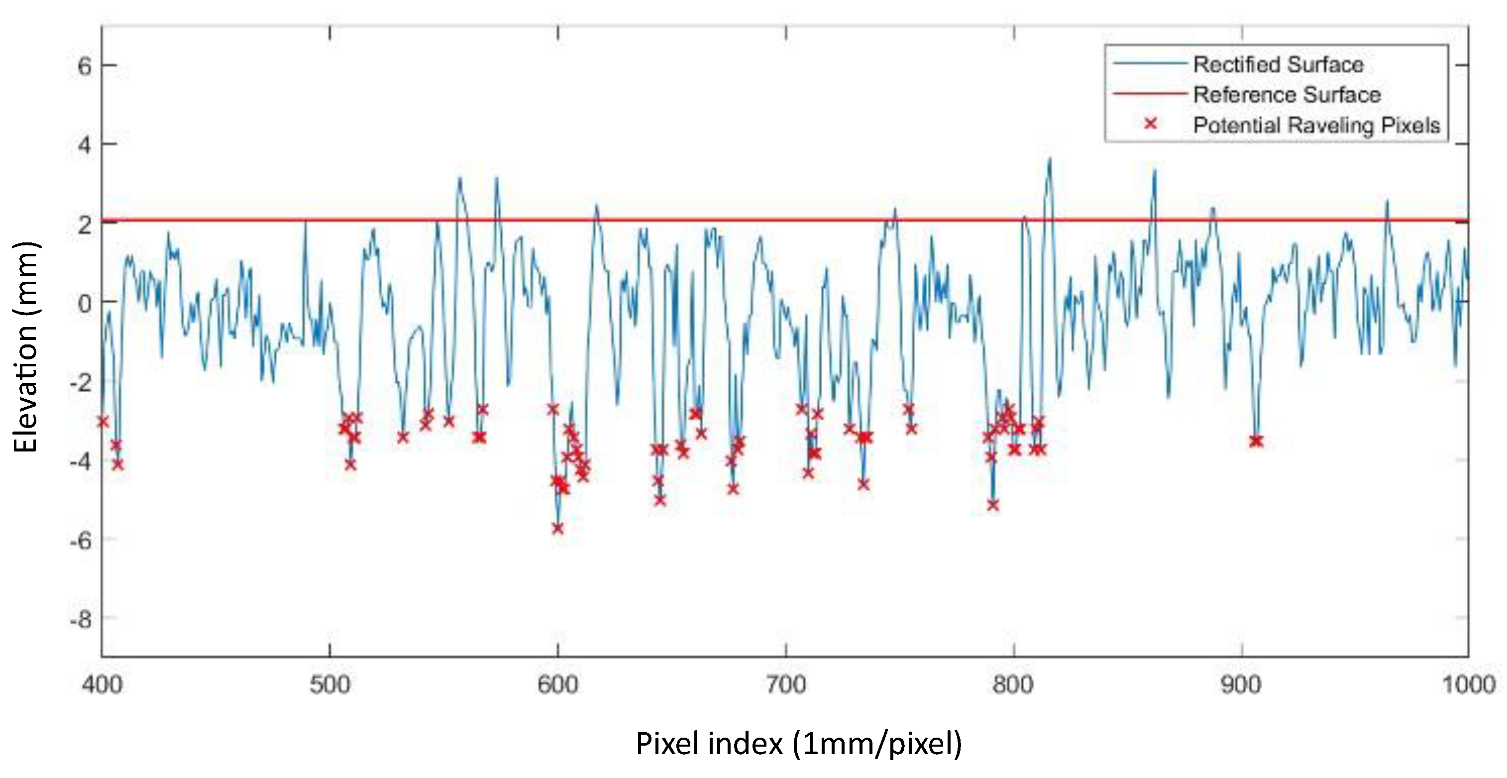
2.3.2. Step 3.2: Use 95th Percentile to Estimate Reference Surface for Each Transverse Profile

The proposed method uses the reference surface to identify and quantify aggregate loss; the reference surface is a smooth surface that represents a pristine surface with no voids and material loss. Such surfaces should intersect with the top surface of aggregates on a brand new pavement. This is shown as the red line in Figure 10. In this step, due to the rectification step, the profiles are “leveled”; rutting and other pavement deformations are removed while the wide raveling areas are preserved. The reference surface can be simplified as a straight line, so the 95th percentile of each rectified transverse profile is used as the reference surface.

2.4. Step 4: Raveling Quantification

2.4.1. Step 4.1: Identify Candidate Pixels of Aggregate Loss

With the reference surface established, each pixel is evaluated. Using simple thresholding, any pixel that is more than 4.75 mm lower than the reference surface is marked as a potential aggregate loss pixel, as shown by the red cross markers in Figure 10. The 4.75 mm threshold was chosen based on the recommended gradation for OGFC, as 75–90% of the aggregate used in OGFC is larger than 4.75 mm in size [21].

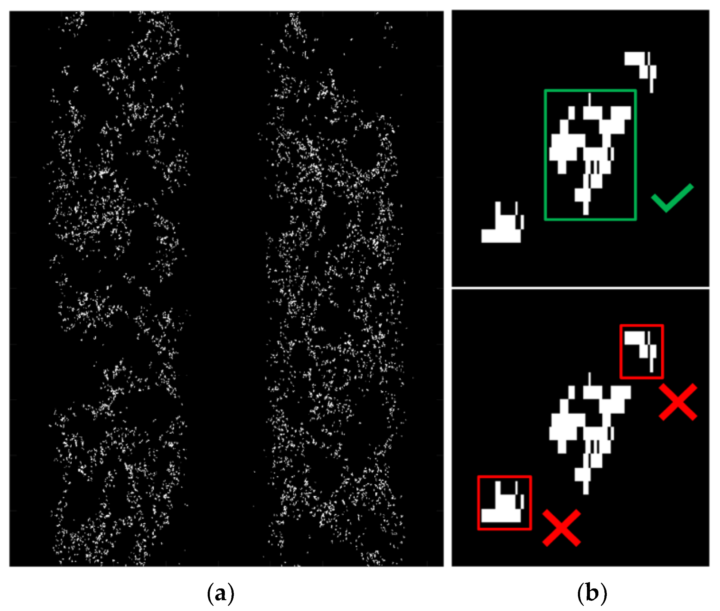
2.4.2. Step 4.2: Analyze Connected Components to Remove Noise

After marking all candidate pixels, a binary image of the pavement, such as shown in Figure 11a, of the pavement can be generated to indicate the locations of all candidate pixels. Because the binary image is obtained through thresholding based on the elevation, the image may contain small surface imperfections or voids between aggregates that should not be considered aggregate loss. To filter out these pixel groups, which are too small to be aggregate loss, each connected component on the binary image is evaluated based on its bounding box sizes. Because aggregate used in OGFC surfaces is typically 4.75–9.5 mm, and dislodged aggregates are likely to have surrounding materials attached, a connected component with a bounding box larger than 10 mm by 10 mm will be accepted as the loss of aggregate, and a bounding box smaller than 10 mm by 10 mm will be rejected. The filtered binary image will be passed down to the next step for loss-of-aggregate quantification.

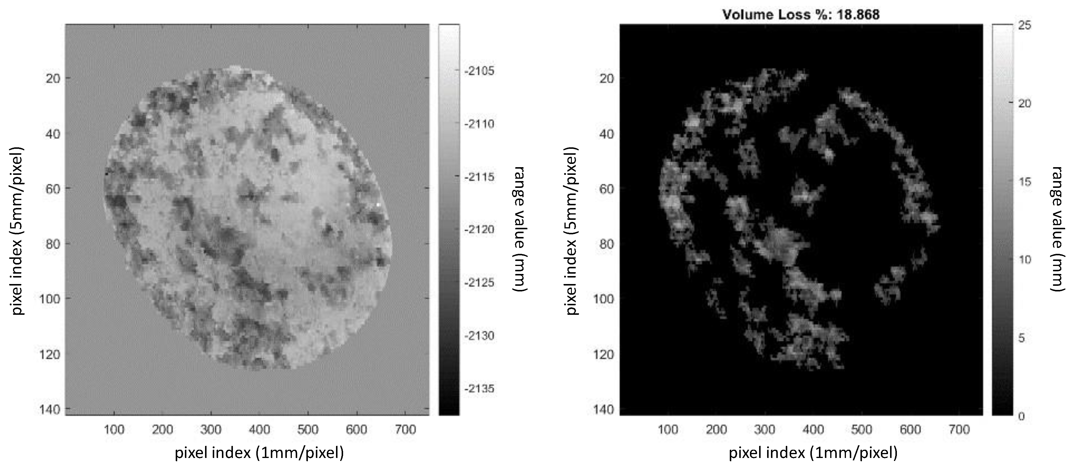
2.4.3. Step 4.3: Aggregate Loss Quantification

Finally, with a filtered binary image, aggregate loss can be quantified. The proposed method quantifies both the percent of the aggregate loss area and the percentage of the aggregate loss volume. The total aggregate loss area ($Los{s}_{area}$) and total aggregate loss volume ($Los{s}_{volume}$) can be expressed as follows:

$$Los{s}_{area}=n_{loss}\times \left(d_t\times d_l\right)$$

(1)

$$Los{s}_{dept{h}_{avg}}={\displaystyle \sum }_{i=1}^{n_{loss}}\frac{\mathsf{\Delta }{e}_i}{n_{loss}}$$

(2)

$$Los{s}_{volume}=Los{s}_{dept{h}_{avg}}\times Los{s}_{area}$$

(3)

where $n_{loss}$ is the number of aggregate loss pixels; $d_t$ and $d_l$ are the sizes of each pixel in terms of real-world dimensions in the transverse and longitudinal directions. $Los{s}_{depth\_avg}$ is the average elevation difference between each aggregate loss pixel and the reference surface, and $\mathsf{\Delta }{e}_i$ is the elevation difference at each aggregate loss pixel to the reference surface.

From $Los{s}_{area}$ and $Los{s}_{volume}$, the percentage of aggregate loss area and the percentage of aggregate loss volume can be computed based on the size of the ROI and the volume of OGFC within the ROI. In addition to the percentage of loss area and percentage of loss volume, the loss volume per unit area can also be an absolute raveling indicator when the information about the pavement thickness is not available. The percentage of loss volume and volume loss per unit area can be expressed as follows:

$$Percen{t}_{Los{s}_{volume}}=\frac{Los{s}_{dept{h}_{avg}}}{OGF{C}_{laye{r}_{thickness}}}\times Percen{t}_{Los{s}_{area}}$$

(4)

$$Uni{t}_{Los{s}_{volume}}=\frac{Los{s}_{volume}}{Are{a}_{pavement}}$$

(5)

3. Validation

Obtaining the true aggregate loss reference from real-world pavement is extremely difficult. In this section, two procedures are presented that aim to develop pavement range data with the known loss of aggregate that can be used to quantitatively evaluate the performance of the proposed method. The first procedure used simulated pavement mats that are fabricated in a lab environment to generate a dataset with the known aggregate loss volume. The second procedure used procedural generation to create a set of synthetic pavement range images with different aggregate loss volumes and areas. Using each dataset, the performance of the proposed method was evaluated critically.

3.1. Validation Using Lab Fabricated Pavement Mat

To quantitatively evaluate the performance of the proposed method, range images with known aggregate loss must be obtained. This paper presents two procedures to establish true aggregate loss references for validation: simulated pavement mats and synthetic pavement range images. The simulated pavement mat, as shown in Figure 12, was fabricated by placing an OGFC aggregate and binder mixture into a small-scale (600 mm diameter) circular pan. The mixture content followed the requirements for an OGFC surface, shown in

Table 1. Aggregate gradation and asphalt content for OGFC surfacing.

Mixture Tolerance	Requirements
	Grading Requirements	Percent Passing
±0.0	3/4 in (19 mm) sieve	100
±6.1	1/2 in (12.5 mm) sieve	85–100
±5.6	3/8 (9.5 mm) sieve	55–75
±5.7	No. 4 (4.75 mm) sieve	15–25
±4.6	No. 8 (2.36 mm) sieve	5–10
±2.0	No. 200 (75 μm) sieve	2–4
	Binder Requirement
±0.4	% Asphalt content	5.75–7.25

. Plaster (mixture of water and gypsum) was used instead of the asphalt so that aggregates could be physically removed easily by hand to simulate raveling. Five sets of range images were scanned; between each set, a fixed volume (170 mL) of aggregate was removed to control the aggregate loss volume. However, the aggregate loss area was still very hard to determine in the fabrication process; thus, it was not recorded. The thickness of the simulated pavement mats was 12.5 mm thick; therefore, each time 170 mL of aggregate was removed, the loss of aggregate volume increased by roughly 5% (4.81% to be exact). Figure 12 shows examples of range images with no aggregate volume loss, 4.81% volume loss, 9.62% volume loss, 14.43% volume loss, and 19.24% volume loss. Due to the size constraint of the simulated pavement mat, pavement features and distresses (such as cross slope and rutting) were not simulated.

Reference images with known aggregate loss were processed using the proposed method to identify locations where the aggregate loss was detected; the aggregate loss is shown as white in Figure 13, and the aggregate loss volume is also quantified. Figure 14 shows the validation results using a simulated pavement mat plotted against their expected values. The proposed method shows promising results, as the aggregate volume loss determined by the proposed method is typically within 2% of the expected values; the correlation coefficient, 0.995, is within the expected values.

3.2. Validation Using Synthetic Pavement Image

Due to the size constraint of the lab-fabricated pavement mat, the effects of cross slope and pavement deformation, such as rutting, on the proposed method were not evaluated. In addition, only the performance of aggregate loss volume quantification was evaluated with the pavement mat; however, the performance of the aggregate loss area quantification should also be evaluated. To address these issues, a MATLAB script was developed to procedurally generate full-scale pavement images with known aggregate loss (Figure 15). The benefits of using synthetic images are as follows: (1) both the aggregate loss area and aggregate loss volume can be controlled; (2) the versatility provided by the synthetic pavement image allows for more pavement images with different raveling conditions to be evaluated (Figure 16); (3) the synthetic pavement can be generated to match the size of a full-scale range image, so cross slope and rutting can also be simulated. The MATLAB script works by using an image of Gaussian white noise to simulate the texture of an OGFC surface and is used as the base surface. Using procedural generation, the location of aggregate loss was defined by a random 2D binary reference image, and the script controlled how the binary image was generated to allow for a higher probability for aggregate loss to occur within the wheel paths and to prevent the generation of pixel groups that were too small to be considered aggregate loss. The elevation values (z-values) of pixels flagged as loss of aggregate were dropped to simulate material loss, and a rougher texture was applied to the areas with aggregate loss. The synthetic surface was then deformed to simulate cross slope and rutting. Finally, random noise was added to the whole image to simulate the image noise from a 3D imaging system.

Using the MATLAB script, 128 synthetic pavement images with different aggregate loss areas and loss volumes were generated. The results in Figure 17a show that the proposed method accurately quantified aggregate loss area in most cases; the validation results and the expected values show a correlation coefficient of 0.997. In areas with a high percentage of loss conditions (around 30–40%), the performance of the proposed method became less stable than in areas with a low percentage of loss conditions, yet the results still have only a ±3% difference from the expected values. The segmentation performance of the proposed method was also evaluated by assigning a buffered Hausdorff distance-based score, which was previously used to evaluate crack segmentation algorithms [22]. The buffered Hausdorff distance-based scoring method was compared to the Hausdorff distance of each detected raveling pixel to the closest raveling pixel in the reference image and assigned a score based on the distance. This method can effectively compare the similarity of segmentation, as a higher Hausdorff distance results in a higher penalty and a lower score. To avoid harsh penalties on small differences in aggregate loss detection, a buffer distance of 1 pixel was used to allow for a small offset in detection, which can still be considered a correct detection. The binary image showing the detected aggregate loss generated by the proposed method was compared with the expected values in the binary image. Figure 17b shows the buffered Hausdorff distance-based scores and the F1 scores of the proposed method on a synthetic dataset. An example of segmentation evaluation is shown in Figure 18, where correctly detected pixels are labeled in white, false positive (FP) detections are labeled in magenta, and false negative (FN) detections are labeled in cyan. The buffered Hausdorff distance-based scores of the proposed method stay above 90 for most cases. The low scores in low-loss area cases were caused by underestimation. However, due to the overall small number of aggregate loss pixels, a small amount of underestimation would cause a big reduction in the score, even though the results from these cases are still very close to the expected values.

As shown in Figure 19, the validation outcomes of quantifying aggregate loss volume also show a strong correlation with the expected values (correlation coefficient = 0.996). The performance of the proposed method was accurate up to around 13%, and after 13% of aggregate volume loss, the results show a small amount of overestimation. This phenomenon is not observed in the simulated pavement mat results. The difference between the two datasets is the inclusion of rutting and cross slope, which suggests the overestimation is related to these features. This error could be introduced during image rectification because, during rectification, a linear profile is assumed to cross each wide-raveling area, as shown in Figure 20, thus making the moving average profile (red line), and, by extension, the reference surface is a straight line across these wide-raveling areas. However, due to the existence of rutting, the reference surface is not a flat surface across the wide-raveling area. Therefore, if the red profile instead of the purple profile were used for rectification, although the loss area will remain mostly unchanged, the loss volume would be overestimated, and such an overestimation would be amplified with a wider wide-raveling area. This theory was confirmed with two additional synthetic image sets, one of which only contained cross slope and one which only contained rutting. As shown in the results in Figure 21, the same overestimation was not observed on the image set that did not have rutting, but it was observed again on the image set that did have rutting. Overall, the impact of the overestimation was limited, and the performance of the proposed method is very promising.

3.3. Performance Comparison with Other Methods

The performance of the proposed method was compared to two other methods, the watershed method [17], and the model fitting method. The watershed method was used in pothole detection and showed promising results. As the name suggests, the watershed method quantifies the loss of aggregate through the surface’s water-holding capacity, as illustrated in Figure 22. The method uses H-minima transformation to capture the notion of the holding capacity on a 3D pavement surface. In theory, by calculating the depth and area of the “water basins”, the aggregate loss can be quantified.

The model fitting method estimates the reference surface on a profile-by-profile basis. The method uses a raw range image, without rectification, and relies on a robust method like Random Sample Consensus (RANSAC) to fit transverse profiles with polynomials with different orders. As shown in Figure 23, the model fitting method uses a combination of first-order and third-order polynomials to segment surface points (red points) to estimate the reference surface.

Using the range images obtained from a simulated pavement mat, the results from both methods are shown in Figure 24. Compared to the proposed method, the watershed method performed poorly; it consistently underestimated the aggregate loss volume. The proposed method and the model fitting method performed comparably until there was an aggregate volume loss of 10%; the accuracy started to drop for the model fitting method after 10%, as the results underestimate the aggregate loss volume. Overall, this shows the proposed method outperformed both other methods in aggregate loss quantification.

The poor performance of the watershed method was likely due to its approach to estimating the reference surface. The method uses average values of a neighborhood to find the reference surface on a 2D plane. As covered in Step 2.2 in Section 2, such an approach is likely to cause underestimation. The proposed method does this on a 2D plane, which means the underestimation is going to affect the reference in the transverse longitudinal directions.

The model fitting method performed better than the watershed method, possibly because the model fitting method uses the robust RANSAC method to fit each transverse profile with first- and third-order polynomials and estimates the reference surface. As long as there is a significant number of data points belonging to the original surface (a surface with no raveling), the RANSAC method should be able to segment surface points for the reference surface estimation. However, as the aggregate loss increases, the number of surface points decreases, and the shape of each transverse profile becomes more and more complex for the polynomials to capture. Therefore, the performance of the RANSEC method becomes worse in high-volume loss conditions.

The proposed method uses low elevation points and sharp slope changes to actively identify wide-raveling areas. With wide-raveling areas identified, the reference surface estimation can be adjusted to account for these areas. Thus, it performs better in low-aggregate loss conditions as well as high-aggregate loss conditions.

4. Conclusions

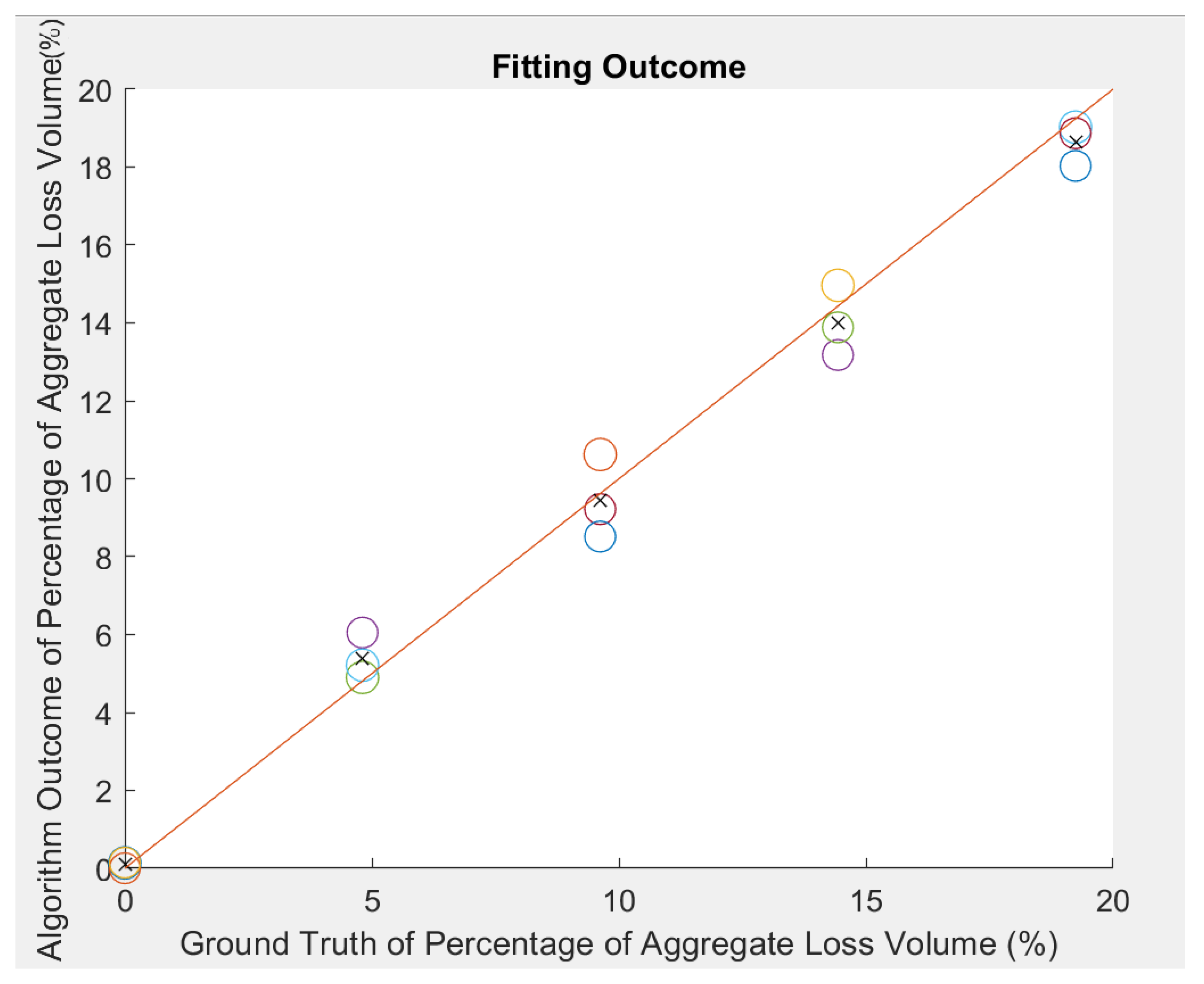
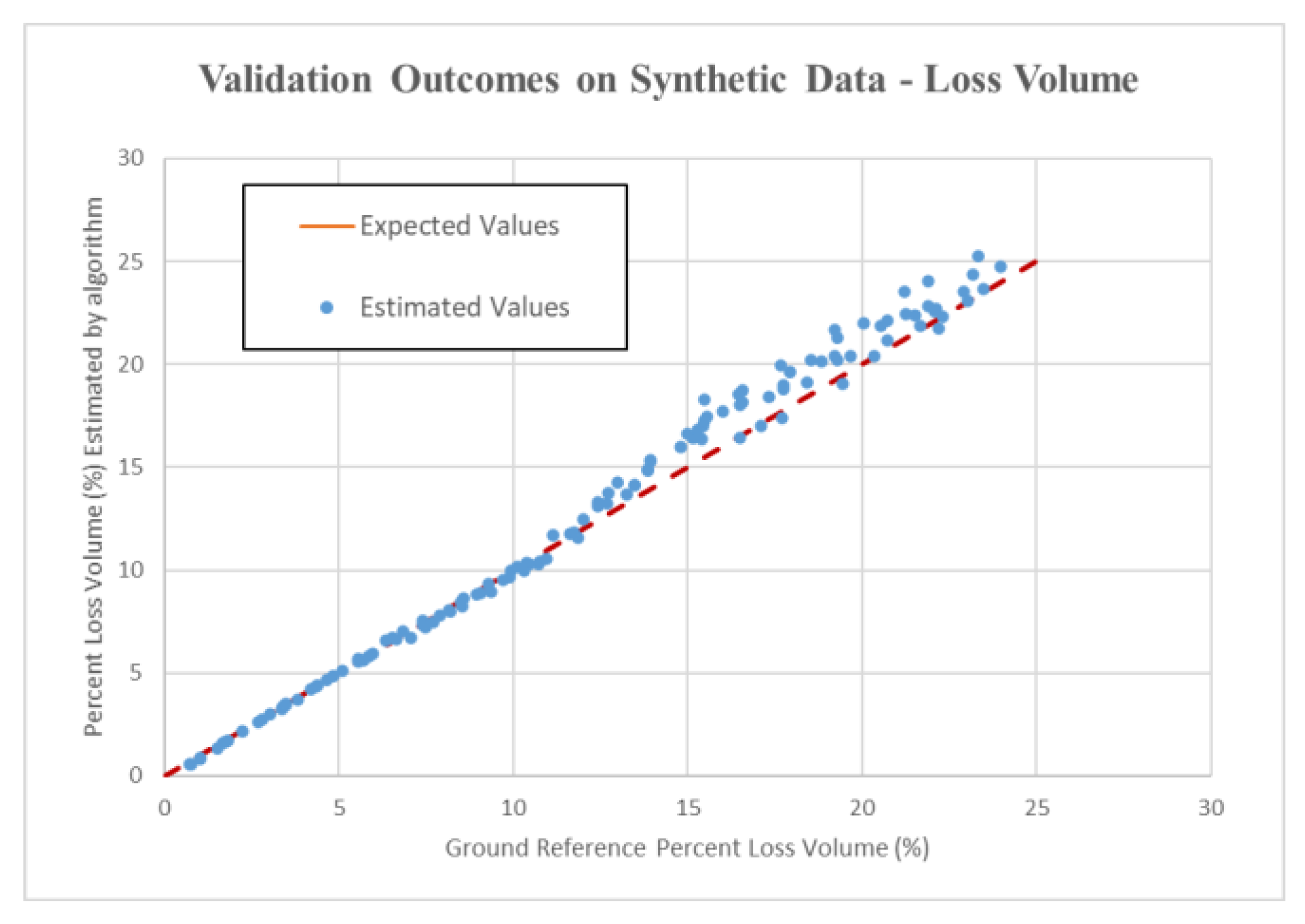
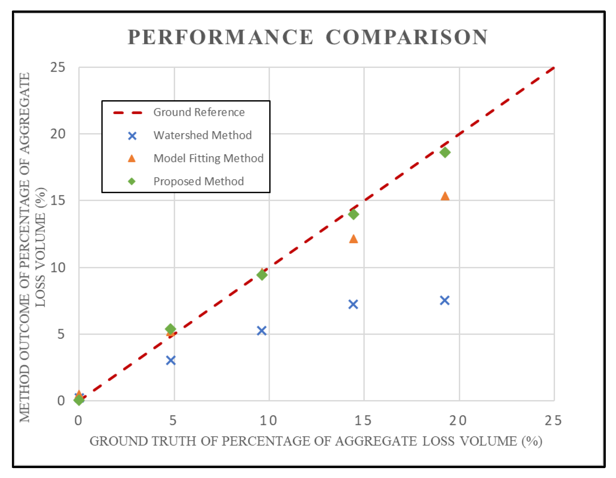
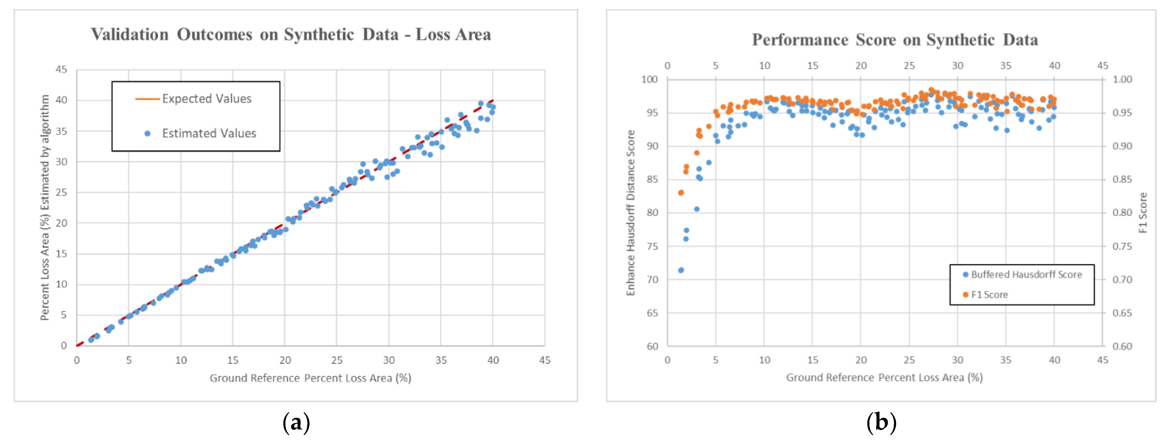
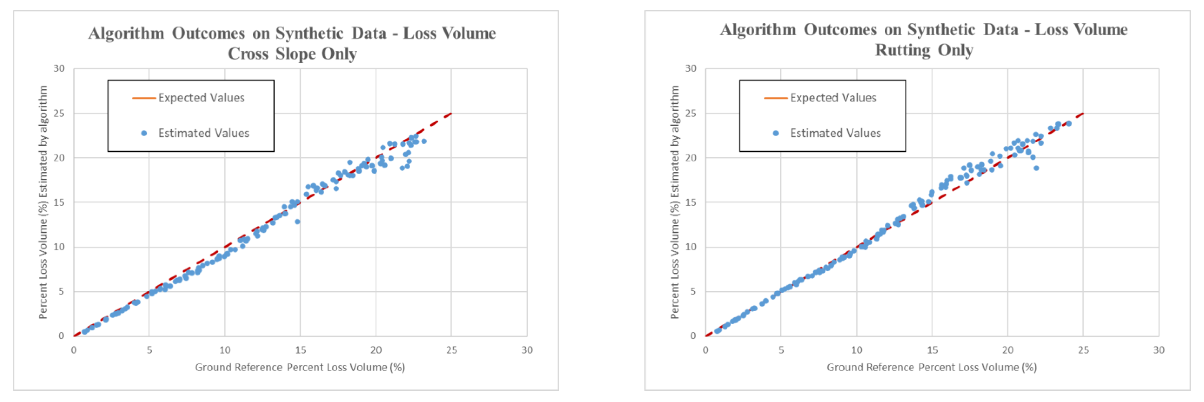
This paper proposes an automatic method, with the loss of aggregate as a new performance indicator, using 3D pavement data to quantitatively measure pavement raveling conditions. The proposed automatic method consists of (1) pavement range data acquisition, (2) pre-processing pavement range images, (3) raveling detection, and (4) raveling quantification. Using lab-fabricated pavement mats and procedurally generated pavement images, the proposed method shows an excellent performance in both aggregate loss volume quantification and aggregate area quantification; the percentages of aggregate loss volumes and areas quantified had less than a 3% difference compared to the expected values. A correlation coefficient of 0.995 was found between the quantified aggregate loss volume and the expected values obtained from the lab-simulated pavement mats. Correlation coefficients of 0.996 and 0.997 were found when comparing the proposed method’s data to expected volume loss and expected area loss obtained from the synthetic pavement data. A critical analysis was also conducted by comparing the performance of the proposed method with other methods (the watershed method and model fitting method). The analysis shows the proposed method had a similar performance to the model fitting method for small percentages of aggregate loss (1–10%); it outperformed other methods in identifying a loss of aggregate between 10% and 20%.

The contribution of the paper includes (1) a loss-of-aggregate quantification method using an enhanced reference surface determination method with wide-raveling identification to resolve the underestimation issue, ensuring the accuracy of the loss-of-aggregate measurement at Severity Level 1, which is the critical range for making pavement preservation decisions, such as applying fog seal; (2) a method to generate synthetic pavement data using a procedurally generated aggregate loss pattern to address the technical challenges in obtaining the loss of aggregate in the field for validation of the proposed method.

5. Recommendations

It is recommended that a standard of using quantitative measures for raveling condition evaluation (nationally and internationally) be determined and established. Such standards could greatly help the development of the quantitative forecasting of raveling to support maintenance scheduling for the application of raveling-specific treatments at the best time. The proposed method is recommended to be used to support the quantitative forecasting of raveling conditions, which has been impossible to achieve until now.

References

1. Onyango, M.; Woods, M. Analysis of the Utilization of Open-Graded Friction Course (OGFC) in the United States. In Airfield and Highway Pavements 2017; ACSE: Reston, VA, USA, 2017; pp. 137–147. [Google Scholar]
2. GDOT. Road Surface Management, Pavement Condition Evaluation System (PACES); GDOT: Atlanta, GA, USA, 1990.
3. FDOT. 2017 Flexible Pavement Condition Survey Handbook; FDOT: Tallahassee, FL, USA, 2017.
4. ODOT. Pavement Data Condition Manual; Oregon Department of Transportation: Salem, OR, USA, 2019.
5. TxDOT. Pavement Management Information System: Rater’s Manual; Texas Department of Transportation: Austin, TX, USA, 2015.
6. Gadsby, A.; Tsai, Y. Environmental Impact of New Micro-Milling and Thin Overlay and Conventional Milling for Sustainable Pavement Preservation. Int. J. Pavement Res. Technol. 2021, 14, 23–29. [Google Scholar] [CrossRef]
7. Tsai, Y.; Wu, Y.; Gadsby, A.; Hines, S. Critical Assessment of the Long-Term Performance and Cost-effectiveness of a New Pavement Preservation Method: Micro-milling and Thin Overlay. Transp. Res. Rec. J. Transp. Res. Board 2016, 2550, 8–14. [Google Scholar] [CrossRef]
8. Tsai, Y.; Wang, Z.; Zhang, X.; Yang, Z. An Enhanced GDOT Pavement Preservation Guide with Optimal Timing of Pavement Preservation; No. FHWA-GA-20-1406; Georgia Department of Transportation, Office of Performance-Based Management & Research: Atlanta, GA, USA, 2021.
9. Zimmerman, K. NCHRP Synthesis 501 Pavement Management Systems: Putting Data to Work; Transportation Research Board of the National Academies: Washington, DC, USA, 2017. [Google Scholar]
10. Tsai, Y.C.J.; Li, F. Critical assessment of detecting asphalt pavement cracks under different lighting and low intensity contrast conditions using emerging 3D laser technology. J. Transp. Eng. 2012, 138, 649–656. [Google Scholar] [CrossRef]
11. Jiang, C.; Tsai, Y.J. Enhanced crack segmentation algorithm using 3D pavement data. J. Comput. Civ. Eng. 2016, 30, 04015050. [Google Scholar] [CrossRef]
12. Jiang, C.; Tsai, Y.; Wang, Z. Crack Deterioration Analysis using 3D Pavement Surface Data: A Pilot Study on Georgia State Route 26. Transp. Res. Rec. 2016, 2589, 154–161. [Google Scholar] [CrossRef]
13. Tsai, Y.J.; Li, F.; Wu, Y. A new rutting measurement method using emerging 3D line-laser-imaging system. Int. J. Pavement Res. Technol. 2013, 6, 667. [Google Scholar]
14. Tsai, Y.J.; Wang, Z.H.; Li, F. Assessment of rut depth measurement accuracy of point-based rut bar systems using emerging 3d line laser imaging technology. J. Mar. Sci. Technol. 2015, 23, 322–330. [Google Scholar]
15. Tsai, Y.J.; Wu, Y.; Ai, C.; Pitts, E. Feasibility study of measuring concrete joint faulting using 3d continuous pavement profile data 2. In Proceedings of the Transportation Research Board 90th Annual Meeting, Washington, DC, USA, 23–27 January 2011. [Google Scholar]
16. Tsai, Y.; Wu, Y.; Lewis, Z. Full-lane coverage micromilling pavement-surface quality control using emerging 3D line laser imaging technology. J. Transp. Eng. 2014, 140, 04013006. [Google Scholar] [CrossRef]
17. Tsai, Y.C.; Chatterjee, A. Pothole detection and classification using 3D technology and watershed method. J. Comput. Civ. Eng. 2018, 32, 04017078. [Google Scholar] [CrossRef]
18. Geary, G.M.; Tsai, Y.; Wu, Y. An Area-Based Faulting Measurement Method Using Three-Dimensional Pavement Data. Transp. Res. Rec. J. Transp. Res. Board 2018, 2672, 41–49. [Google Scholar] [CrossRef]
19. Mathavan, S.; Rahman, M.M.; Stonecliffe-Jones, M.; Kamal, K. Pavement raveling detection and measurement from synchronized intensity and range images. Transp. Res. Rec. J. Transp. Res. Board 2014, 2457, 3–11. [Google Scholar] [CrossRef] [Green Version]
20. Laurent, J.; Hébert, J.F.; Lefebvre, D.; Savard, Y. Using 3D laser profiling sensors for the automated measurement of road surface conditions. In Proceedings of the 7th RILEM International Conference on Cracking in Pavements, Delft, The Netherlands, 20–22 June 2012; pp. 157–167. [Google Scholar]
21. Kandhal, P.S. Design, Construction, and Maintenance of Open-Graded Asphalt Friction Courses; National Asphalt Pavement Association: Greenbelt, MD, USA, 2002. [Google Scholar]
22. Kaul, V.; Tsai, Y.; Mersereau, R.M. Quantitative performance evaluation algorithms for pavement distress segmentation. Transp. Res. Rec. J. Transp. Res. Board 2010, 2153, 106–113. [Google Scholar] [CrossRef]
Figure 1. Flowchart of the proposed method.
Sustainability 14 07471 g001
Figure 2. (a) Georgia Tech Sensing Vehicle equipped with sensors and (b) pavement range data collected by 3D laser system.
Sustainability 14 07471 g002
Figure 3. Pavement range data before and after smoothed using a Gaussian filter.
Sustainability 14 07471 g003
Figure 4. (a) Original range image, (b) rectified range image.
Sustainability 14 07471 g004
Figure 5. (a) Top: Moving average without wide-raveling identification. (b) Bottom: Moving average with wide-raveling identification.
Sustainability 14 07471 g005aSustainability 14 07471 g005b
Figure 6. Wide-raveling identification process.
Sustainability 14 07471 g006
Figure 7. Top-down view of the sensor setup and yaw angle of the laser lines.
Sustainability 14 07471 g007
Figure 8. Rectified range image collected: (a) left sensor, (b) right sensor, (c) stitched image.
Sustainability 14 07471 g008
Figure 9. Pavement intensity image and regions of interest for aggregate loss detection.
Sustainability 14 07471 g009
Figure 10. Reference surface estimation and potential aggregate loss identification.
Sustainability 14 07471 g010
Figure 11. (a) Binary image of potential aggregate loss. (b) Top right: example of accepted connected components. Bottom right: examples of rejected connected components.
Sustainability 14 07471 g011
Figure 12. Simulated pavement mat and collected range images with different volumes of aggregate loss. From left to right, top to down: (a) image of simulated pavement mat, (bf) range image of mat with aggregate loss of 0–20%.
Sustainability 14 07471 g012
Figure 13. Range image with 19.24% volume loss processed using proposed method.
Sustainability 14 07471 g013
Figure 14. Quantified percentage of aggregate loss (y-axis) vs. expected values (x-axis).
Sustainability 14 07471 g014
Figure 15. Example of a synthetic pavement image and a binary reference image indicating locations with aggregate loss.
Sustainability 14 07471 g015
Figure 16. Binary reference images of synthetic pavements with different levels of aggregate loss.
Sustainability 14 07471 g016
Figure 17. (a) Left: Validation outcomes of aggregate loss area using synthetic dataset, (b) right: buffered Hausdorff distance-based score and F1 score on synthetic dataset.
Sustainability 14 07471 g017
Figure 18. Evaluation of the segmentation performance. Left: Rectified range image. Middle: Color coded image to show FP and FN detections. Right: Reference binary image.
Sustainability 14 07471 g018
Figure 19. Validation outcomes of aggregate loss volume using synthetic dataset.
Sustainability 14 07471 g019
Figure 20. Illustration of aggregate loss volume overestimation caused by rutting over a wide-raveling area.
Sustainability 14 07471 g020
Figure 21. Validation outcomes of aggregate loss volume. Left: Synthetic pavement images with no rutting. Right: Synthetic pavement images with rutting.
Sustainability 14 07471 g021
Figure 22. Illustration of the watershed method.
Sustainability 14 07471 g022
Figure 23. Illustration of the model fitting method. Left: Surface points segmented by third−order polynomial. Middle: Surface points segmented by first−order polynomial. Right: Combined surface points.
Sustainability 14 07471 g023
Figure 24. Performance comparison between the watershed method, the model fitting method, and the proposed method.
Sustainability 14 07471 g024