Estimation of Ground Thermal Properties of Shallow Coaxial Borehole Heat Exchanger Using an Improved Parameter Estimation Method

Abstract

Ground thermal properties are prerequisites for designing the size of borehole heat exchanger. In this study, a 3D heat transfer model is developed to simulate the thermal response test (TRT) of shallow coaxial borehole heat exchanger (SCBHE), and effects of ground thermal properties on the slope of the mean value of inlet and outlet fluid temperatures are studied. The results show that the slope is strongly affected by ground thermal conductivity and is slightly affected by ground thermal capacity, and that ground thermal capacity only has a small effect on the slope. Then, by using the difference between the experimental slope and calculated slope as the objective function to estimate ground thermal conductivity, an improved parameter estimation method (PEM) is proposed to estimate ground thermal properties of SCBHE using the simulated TRT data, and it is compared with the direct method. The results show that ground thermal conductivity and thermal capacity estimated by the improved PEM are accurate for different ground thermal properties, and that ground thermal conductivity estimated by the direct method probably has some errors especially for small ground thermal conductivity or thermal capacity, indicating that the improved PEM has much higher precision than the direct method and can be applied for estimating the ground thermal properties of SCBHE.

1. Introduction

As a common kind of geothermal heat exchanger, borehole heat exchanger (BHE) is an important part of ground-source heat pump (GSHP), which accounts for the largest installed capacity of geothermal direct utilization worldwide [1,2]. Because of having great effects on the performance and cost of GSHP, the design of BHE is very necessary, the key parameters of which are the ground thermal properties [3,4].

There are mainly four methods to measure ground thermal properties, i.e., in situ probes, experimental testing of ground samples, soil and rock identification, and thermal response test (TRT) [5]. The in situ probes and experimental testing of ground samples adopt some apparatus to measure the ground thermal properties directly, but the measured values can hardly represent the real values of ground for BHE and probably have large errors [6]. Soil and rock identification method uses empirical or theoretical models to estimate the ground thermal properties based on some parameters such as rock type and water content [7], however, this method is limited under certain conditions [8]. By simulating the actual heat transfer process of BHE, TRT measures the fluid temperature distribution, and then estimates the ground thermal properties based on heat transfer models and parameter identification methods [5]. Because of having higher precision than the other methods, TRT has become the most common method for estimating the ground thermal properties of BHE [6]. Parameter identification method is very important to estimate accurate ground thermal properties by using TRT data analysis [9].

Parameter identification method includes two methods, i.e., direct method and parameter estimation method (PEM). The theory of direct method is infinite line source (ILS) model which solves the heat transfer problem of an infinite line source in the ground, and the result of ILS model shows that ground thermal conductivity tends to be proportional to the slope of the linear equation about the mean fluid temperature (normally assumed as the average of inlet and outlet fluid temperatures) and logarithm of time [10]. Therefore, ground thermal conductivity can be calculated by linear fitting of TRT data, besides, the borehole resistance can also be calculated simultaneously [6]. Direct method is being widely used in practical engineering design, however, it has some shortcomings: the relationship between mean fluid temperature and logarithm of time may not be linear especially at the early time, the start of the linear relationship may not be clear, and the method is only suitable for constant heat input rate [5].

PEM solves an inverse problem to estimate ground thermal properties by matching TRT data and heat transfer models of BHE [9]. Accurate heat transfer model is crucial to enhance the precision of PEM, therefore, more accurate heat transfer models have been studied [11], such as composite-medium line source model [12], and improved cylindrical source model which takes the borehole thermal capacity into account [13]. Generally, the root mean squared error (RMSE) or sum of squared errors (SSE) of mean fluid temperature is selected as the objective function of the inverse problem [9], but some researchers have also investigated the SSE or RMSE of mean fluid temperature derivative as the objective function, and find that the new objective functions can improve the precision of estimated ground thermal capacity and reduce the correlation and uncertainty of estimated parameters [14,15]. The mean fluid temperature of BHE is normally assumed to be the average of inlet and outlet fluid temperatures, which would reduce the estimation precision, and some researchers developed more accurate methods to calculate the mean fluid temperature [8,16]. Besides, two-step or multi-step PEMs are studied by using several steps to estimate the unknown parameters respectively: according to the results of sensitivity analysis, different TRT data can be used to estimate different parameters respectively, and more parameters can be estimated accurately [17,18]; estimation sequence can also influence the precision of PEM [19]; estimation precision of PEM can be further improved by using different objective functions which are related to different TRT data [20].

Shallow coaxial BHE (SCBHE) is an important kind of BHE [4], however, Beier et al. [21,22] and Morchio et al. [23] found that there would exist a large difference between the actual mean fluid temperature and the average of inlet and outlet fluid temperatures for SCBHE, and that the direct method may have large errors for estimating the unknown parameters of SCBHE. Besides, only a few studies have been conducted on the PEM of SCBHE by using two-step PEMs [19,20] or more accurate heat transfer models [21,22], however, the objective functions of these studies are RMSE of fluid temperatures, and there is some potential to improve the estimation precision and reliability of PEM by using other objective functions. This paper firstly develops a 3D heat transfer model to simulate the TRT of SCBHE based on FLUENT software, and then studies the effects of ground thermal properties on the slope of the average of inlet and outlet fluid temperatures, then an improved PEM is proposed by using the difference between experimental and calculated slopes as the objective function, and finally the improved PEM is verified based on the simulated TRT data.

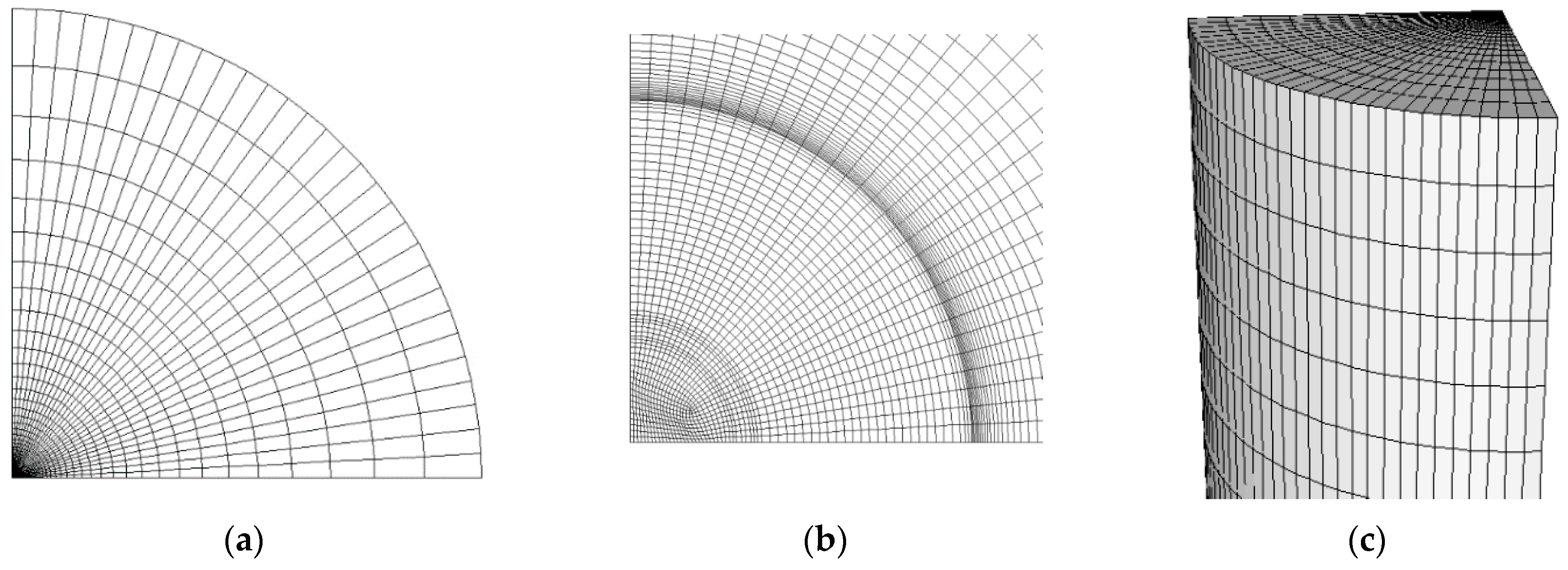
2. 3D Heat Transfer Model of SCBHE

By using FLUENT software, a 3D heat transfer model can be established to model the TRT of SCBHE, the parameters of which are consistent with those of the TRT conducted by Acuña et al. [24], as presented in

Table 1. Detailed parameters of SCBHE [24].

Parameter	Value
SCBHE length L (m)	168
Borehole radius rb (m)	0.0575
Internal radius of internal pipe rii (m)	0.0176
External radius of internal pipe rie (m)	0.020
Internal radius of external pipe rei (m)	0.0566
External radius of external pipe ree (m)	0.057
Thermal conductivities of internal and external pipes λip, λep (W·m−1·K−1)	0.4
Thermal capacities of internal and external pipes (ρc)ip, (ρc)ep (J·m−3·K−1)	1.8 × 106
Grout thermal conductivity λg (W·m−1·K−1)	0.59
Grout thermal capacity (ρc)g (J·m−3·K−1)	4.19 × 106
Ground thermal conductivity λgr (W·m−1·K−1)	3.28
Ground thermal capacity (ρc)gr (J·m−3·K−1)	2.24 × 106
Fluid thermal conductivity λf (W·m−1·K−1)	0.59
Fluid thermal capacity (ρc)f (J·m−3·K−1)	4.19 × 106
Fluid Prandtl number Pr	8.09
Initial ground temperature T0 (℃)	8.4
Fluid flow rate V (m3·s−1)	0.58 × 10−3
Heat input rate of SCBHE Qin (W)	6360

.

The heat transfer in the ground, grout, external pipe and internal pipe is pure heat conduction, and the partial differential equation of heat conduction can be applied. The fluid flow can be modeled using the standard k-ε model. So the TRT of SCBHE can be simulated by FLUENT software. To simplify the SCBHE, the lengths of internal pipe and external pipe are assumed to be equal, as shown in Figure 1. By using User Defined Function, the inlet temperatures of internal and annular fluids are set as follows:

$$T_{\mathrm{i}}\left(z=0,t\right)=T_{\mathrm{a}}\left(z=0,t\right)+\frac{Q_{\mathrm{in}}}{V{(\rho c)}_{\mathrm{f}}}$$

(1)

$$T_{\mathrm{a}}\left(z=L,t\right)=T_{\mathrm{i}}\left(z=L,t\right)$$

(2)

where T_i and T_a are the temperatures of internal and annular fluids respectively, °C; t is the time, s; z is the vertical coordinate, m; Q_in is the heat input rate of SCBHE, W; V is the fluid flow rate, m³·s⁻¹; (ρc)_f is the fluid thermal capacity, J·m⁻³·K⁻¹; L is the SCBHE length, m.

Because the above BHE is symmetric, only a quarter of it is considered, and the geometry can be meshed, shown in Figure 2, and then it is simulated based on FLUENT software.

The above 3D heat transfer model is validated by comparison with experimental results of TRT [24], as shown in Figure 3. The inlet and outlet fluid temperatures simulated by the 3D heat transfer model agree well with the experimental results, but there also exist some differences between them, which are caused by the fact that the actual heat input rate during the TRT is not constant and varies with time.

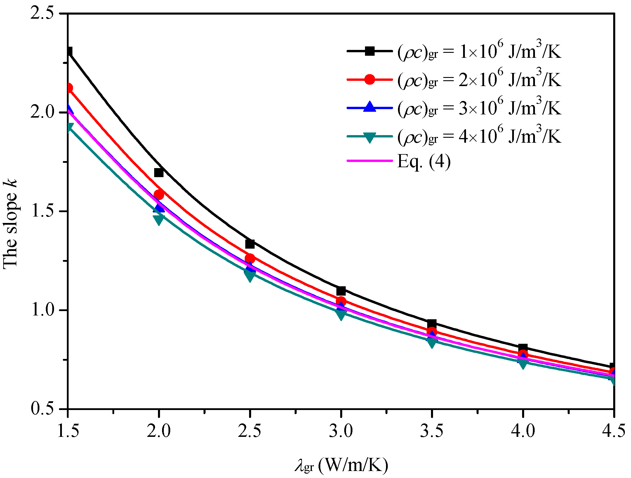
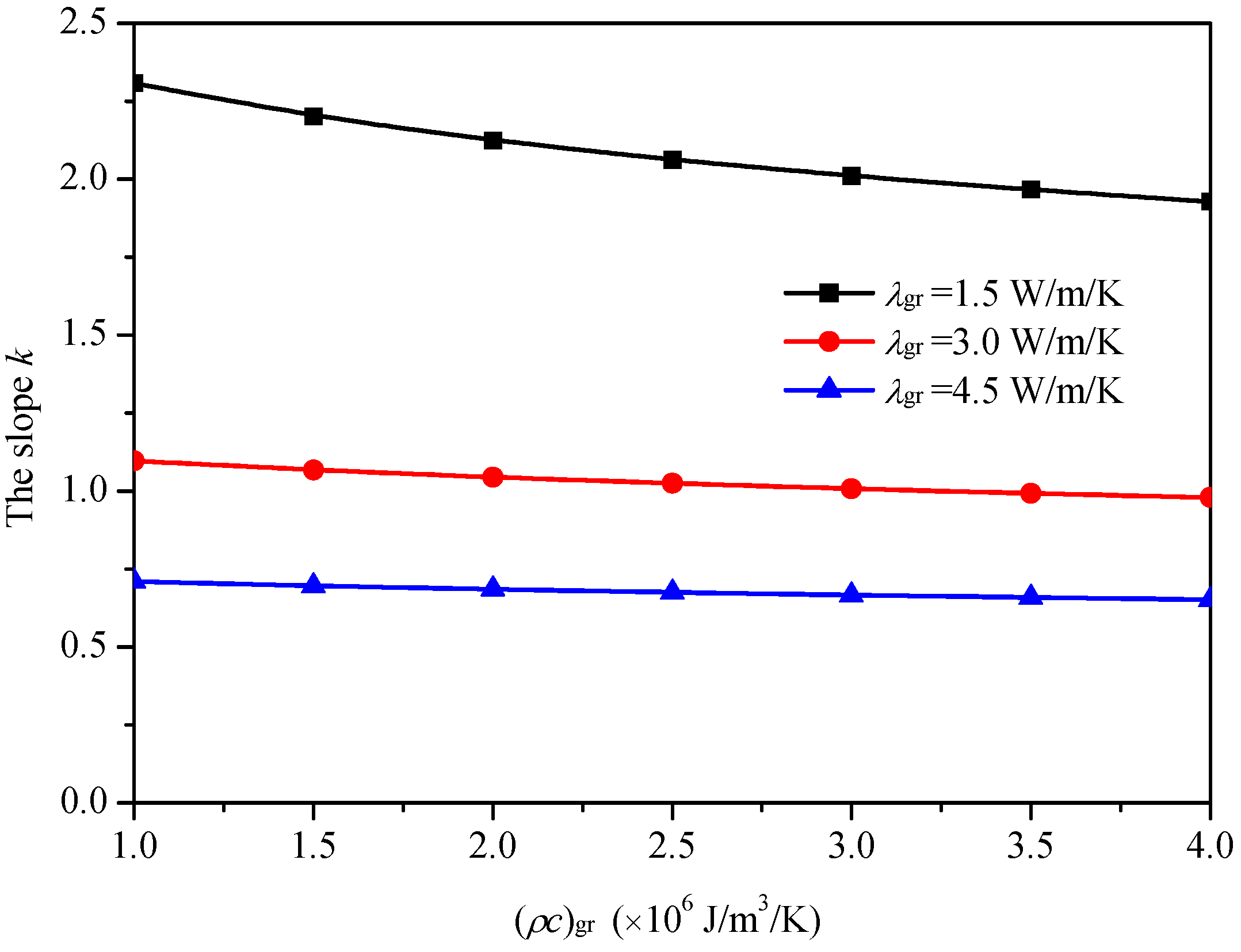
3. Effects of Ground Thermal Properties on the Slope

Based on the verified 3D heat transfer model, TRT of SCBHE at different ground thermal properties is simulated, and effects of ground thermal properties on the slope are investigated based on the simulated TRT data.

According to the ILS model, the slope (k) meets the following equations [6]:

$$T_{\mathrm{f}}\left(t\right)=k\ln \left(t\right)+b$$

(3)

$$k=\frac{Q_{\mathrm{in}}}{4\pi L{\lambda }_{\mathrm{gr}}}$$

(4)

where T_f is the mean fluid temperature of SCBHE, °C; b is the intercept of the linear Equation (3); λ_gr is the ground thermal conductivity, W·m⁻¹·K⁻¹. In practical TRT, inlet and outlet fluid temperatures of SCBHE are generally measured, therefore, the direct method normally regards the average of inlet and outlet fluid temperatures as the mean fluid temperature, and calculates k by linear fitting of Equation (3), and then uses Equation (4) to calculate the ground thermal conductivity. It should be mentioned that the slope k in this paper means the slope of Equation (3), in which T_f is regarded as the average of inlet and outlet fluid temperatures of SCBHE, and that the early-time (normally the first 10 h) TRT data are ignored when using linear fitting of Equation (3).

Figure 4 shows the effect of ground thermal conductivity on the slope at different ground thermal capacities. The result shows that the slope decreases about 66.2–69.2% when the ground thermal conductivity increasing from 1.5 to 4.5 W·m⁻¹·K⁻¹, meaning that ground thermal conductivity has a great effect on the slope, however, the relationship between the slope and ground thermal conductivity probably does not satisfy Equation (4). As shown in Figure 4, it is only when (ρc)_gr equals to about 3 × 10⁶ J·m⁻³·K⁻¹ that the relationship between the slope and ground thermal conductivity satisfies Equation (4) well, and there is larger difference between the relationship and Equation (4) for smaller ground thermal conductivity. For smaller ground thermal conductivity or thermal capacity, the mean fluid temperature increases more quickly with time and the effect of measurement error is smaller, but the effect of borehole thermal capacity is larger, which means that the error of ILS model is larger and ground thermal conductivity estimated by Equation (4) has larger error, so the difference between the relationship and Equation (4) is influenced by the two aspects which are mainly determined by ground thermal conductivity and thermal capacity.

Figure 5 presents the effect of ground thermal capacity on the slope at different ground thermal conductivities. The result shows that the slope decreases about 8.3%-16.5% when the ground thermal capacity increases from 1.0 × 10⁶ to 4.0 × 10⁶ J·m⁻³·K⁻¹, and that ground thermal capacity has a larger effect on the slope for smaller ground thermal conductivity, meaning that the ground thermal capacity only has a small effect on the slope.

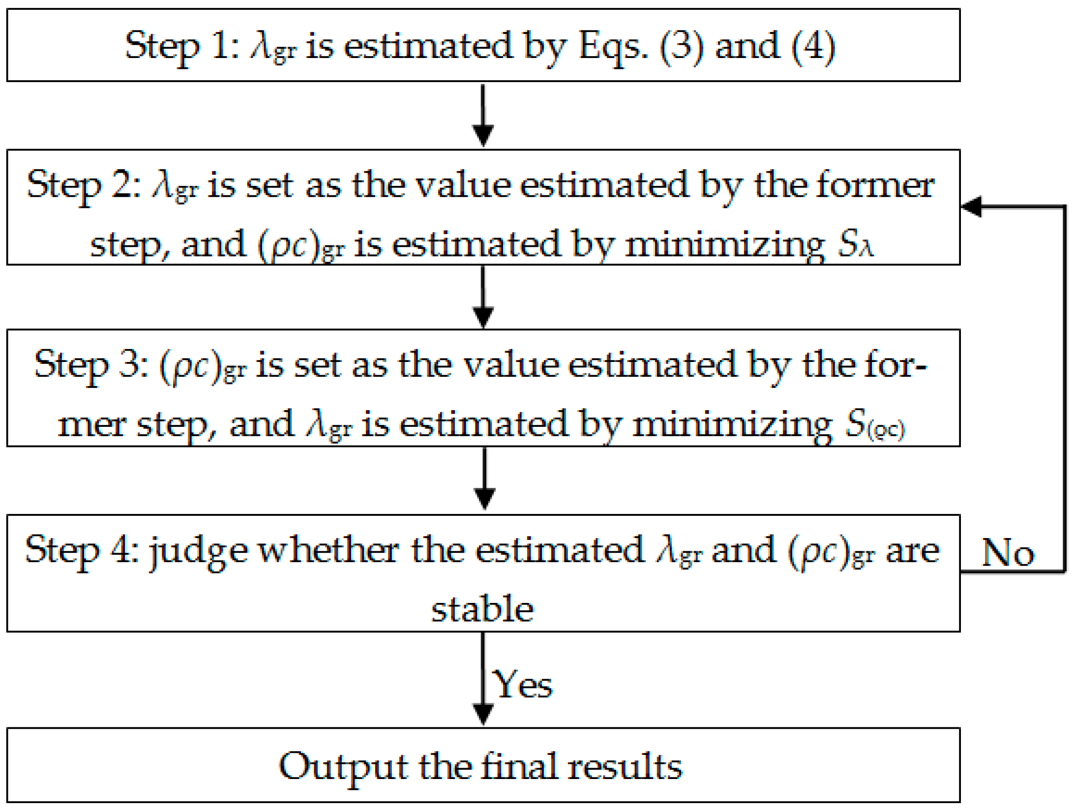
4. Improved Parameter Estimation Method

The above results show that the slope is strongly affected by ground thermal conductivity and is slightly affected by ground thermal capacity, and that ground thermal conductivity calculated by the direct method may have a large error. Therefore, this paper proposes the following objective function to estimate the ground thermal conductivity:

$$S_{\mathsf{\lambda }}=\left|k_{\mathrm{e}}-k_{\mathrm{c}}\right|$$

(5)

where k_e is the slope of Equation (3) about the average of inlet and outlet fluid temperatures of TRT, and k_c is the slope of Equation (3) about the average of inlet and outlet fluid temperatures calculated by heat transfer model.

The objective function to estimate the ground thermal capacity is given as follows [20]:

$$S_{\left(\mathsf{\rho }\mathrm{c}\right)}=\sqrt{\frac{1}{2M}{\displaystyle \sum _{i=1}^M\left[{\left(T_{\mathrm{ci},\mathrm{i}}-T_{\mathrm{ei},\mathrm{i}}\right)}^2+{\left(T_{\mathrm{co},\mathrm{i}}-T_{\mathrm{eo},\mathrm{i}}\right)}^2\right]}}$$

(6)

where M is the M-th test time for t = 10 h; T_ci,i and T_ei,i are the calculated and experimental inlet fluid temperatures at the i-th test time respectively, °C; T_co,i and T_eo,i are the calculated and experimental outlet fluid temperatures at the i-th test time respectively, °C.

Therefore, by using the heat transfer model presented in our previous work [25,26] and introduced in the Appendix A, an improved PEM (shown in Figure 6) can be proposed as follows:

Step 1: the direct method is used to estimate λ_gr (ground thermal conductivity) based on Equations (3) and (4).

Step 2: ground thermal conductivity in the former step is taken as the known value, and (ρc)_gr (ground thermal capacity) is estimated by minimizing S_(ρc) based on Monte Carlo method [20]. It should be mentioned that S_(ρc) is the objective function about the inlet and outlet fluid temperatures estimated by the heat transfer model [25] and those of TRT data.

Step 3: ground thermal capacity in the former step is taken as the known value, and λ_gr is estimated by minimizing S_λ based on Monte Carlo method. It should be mentioned that S_λ is the objective function about k_e and k_c, and that k_c is calculated based on the heat transfer model in Ref. [25].

Step 4: Steps 2 and 3 are repeated until the estimated results are stable.

The purpose of Step 1 is to estimate a relatively accurate value of ground thermal conductivity, which would reduce the computation time of the improved PEM. The differences between the improved PEM and the direct method are as follows: 1) the direct method adopts Equations (3) and (4) to estimate λ_gr directly, while the improved PEM adopts an iterative algorithm (i.e., Monte Carlo method) to estimate λ_gr by minimizing the difference between k_e and k_c; (2) the direct method assumes that the mean fluid temperature equals to the average of inlet and outlet fluid temperatures, while the improved PEM has no such assumption; (3) the direct method is not able to estimate (ρc)_gr, while the improved PEM can also estimate (ρc)_gr.

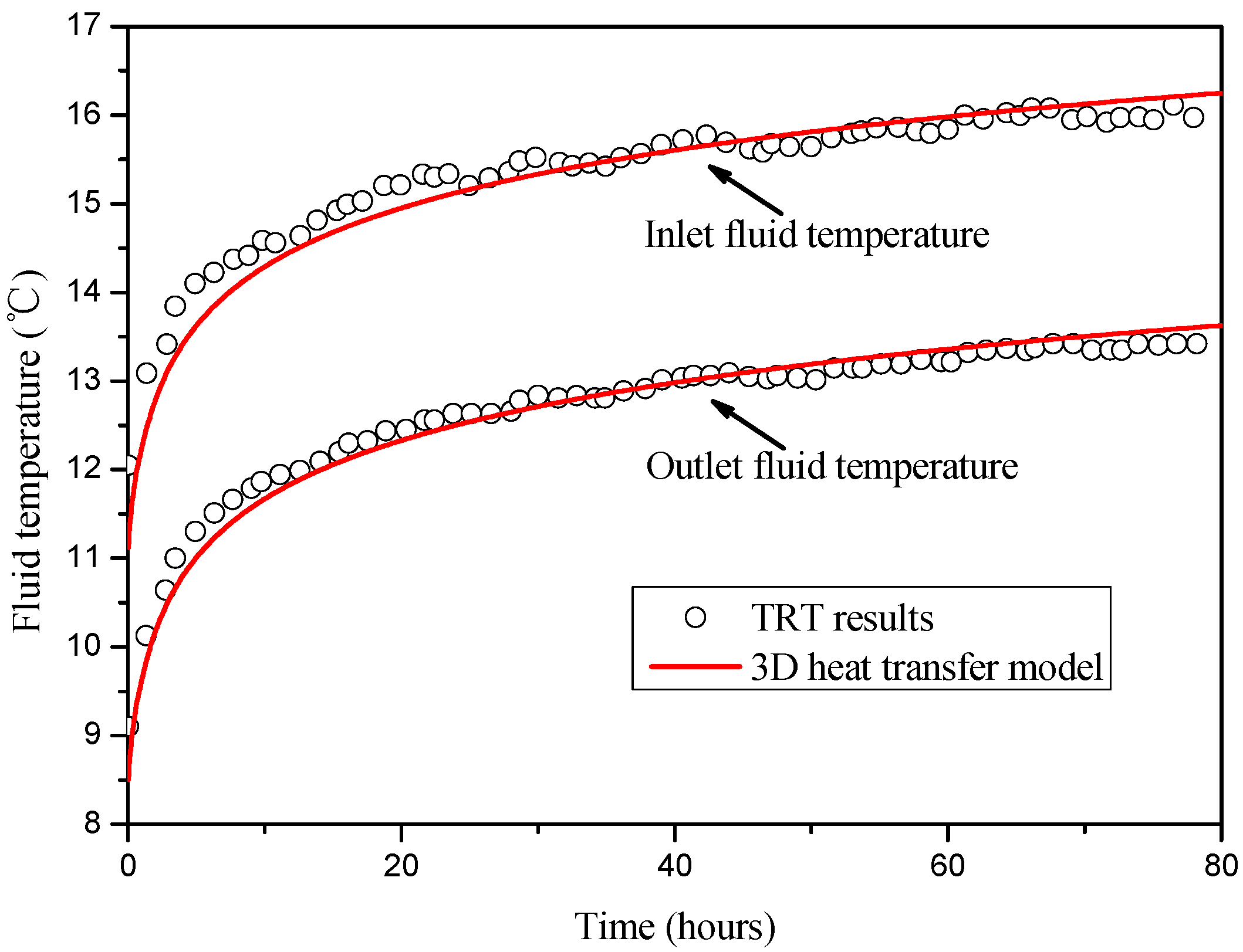
5. Results and Discussion

To verify the improved PEM, it is used to estimate the ground thermal properties of the SCBHE presented in Section 2 based on the simulated TRT data, and it is compared with the direct method. The total time of the simulated TRT is 50 h, and the early 10-h data are ignored when calculating the slopes [8].

Table 2. Comparison of the reference values of ground thermal properties with the results calculated by the improved PEM and direct method.

Reference Values		Calculated Results of Direct Method		Calculated Results of the Improved PEM
(ρc)gr (×106 J·m−3·K−1)	λgr (W·m−1·K−1)	λgr (W·m−1·K−1)	Error of λgr	λgr (W·m−1·K−1)	Error of λgr	(ρc)gr (×106 J·m−3·K−1)	Error of (ρc)gr
1.0	1.5	1.306	12.9%	1.490	0.7%	1.001	0.1%
1.0	2.0	1.777	11.2%	1.987	0.7%	1.008	0.8%
1.0	2.5	2.258	9.7%	2.489	0.4%	1.005	0.5%
1.0	3.0	2.746	8.5%	2.985	0.5%	1.002	0.2%
1.0	3.5	3.239	7.5%	3.485	0.4%	1.005	0.5%
1.0	4.0	3.737	6.6%	3.985	0.4%	1.006	0.6%
1.0	4.5	4.239	5.8%	4.482	0.4%	1.011	1.1%
2.0	1.5	1.419	5.4%	1.491	0.6%	2.013	0.7%
2.0	2.0	1.903	4.9%	1.990	0.5%	2.002	0.1%
2.0	2.5	2.392	4.3%	2.490	0.4%	1.999	0.1%
2.0	3.0	2.887	3.8%	2.987	0.4%	2.007	0.4%
2.0	3.5	3.388	3.2%	3.485	0.4%	2.019	1.0%
2.0	4.0	3.893	2.7%	3.980	0.5%	2.021	1.1%
2.0	4.5	4.401	2.2%	4.480	0.4%	2.026	1.3%
3.0	1.5	1.499	0.1%	1.495	0.3%	3.005	0.2%
3.0	2.0	1.991	0.5%	1.992	0.4%	3.007	0.2%
3.0	2.5	2.488	0.5%	2.490	0.4%	3.010	0.3%
3.0	3.0	2.990	0.3%	2.990	0.3%	3.004	0.1%
3.0	3.5	3.496	0.1%	3.490	0.3%	3.012	0.4%
3.0	4.0	4.007	0.2%	3.990	0.3%	3.016	0.5%
3.0	4.5	4.522	0.5%	4.481	0.4%	3.038	1.3%
4.0	1.5	1.563	4.2%	1.502	0.1%	3.971	0.7%
4.0	2.0	2.063	3.1%	1.998	0.1%	3.979	0.5%
4.0	2.5	2.567	2.7%	2.496	0.2%	3.980	0.5%
4.0	3.0	3.075	2.5%	2.995	0.2%	3.996	0.1%
4.0	3.5	3.587	2.5%	3.492	0.2%	4.009	0.2%
4.0	4.0	4.103	2.6%	3.988	0.3%	4.027	0.7%
4.0	4.5	4.623	2.7%	4.480	0.4%	4.056	1.4%

presents the comparison of the reference values of ground thermal properties with the results calculated by the improved PEM and direct method, and to give a better comparison of the two methods, the data of Table 2 are plotted in Figure 7. The direct method would estimate λ_gr accurately when (ρc)_gr equals to about 3.0 × 10⁶ J·m⁻³·K⁻¹, and would overestimate λ_gr when both λ_gr and (ρc)_gr are large enough, and would underestimate λ_gr when λ_gr or (ρc)_gr is small enough. The main reasons for the errors of direct method are as follows: there exist certain errors when using the ILS model for analyzing the heat transfer in the SCBHE; the assumption of using the average of inlet and outlet fluid temperatures to approximate the mean fluid temperature would also lead to some errors. The precision of the direct method is very high for (ρc)_gr = 3.0 × 10⁶ J·m⁻³·K⁻¹, which is because the relationship between the slope and ground thermal conductivity satisfies Equation (4) well for the given conditions, shown in Figure 4.

The improved PEM can estimate λ_gr and (ρc)_gr accurately for all the situations presented in Table 2, and the errors of the estimated λ_gr and (ρc)_gr are within 0.7% and within 1.4% respectively, indicating that the improved PEM has high precision, which is explained as follows: the heat transfer model used in the improved PEM considers the borehole thermal capacity, and has high accuracy [25,26]; there is no assumption about the mean fluid temperature; because of the strong effect of ground thermal conductivity on the slope, the objective function about the difference between the experimental slope and calculated slope can be used for estimating the ground thermal conductivity accurately; because the ground thermal capacity has a larger effect on the early-time fluid temperatures than on the later-time fluid temperatures, the objective function in Eq. (6) is used to estimate an accurate ground thermal capacity.

The results indicate that the direct method may have large errors especially for small ground thermal conductivity or thermal capacity, and that the improved PEM can estimate the ground thermal conductivity and thermal capacity accurately for different ground thermal properties.

6. Conclusions

In this study, a 3D heat transfer model is developed to simulate the TRT of SCBHE based on FLUENT software, and then it is validated by comparison with experimental data. Based on the verified 3D heat transfer model, effects of the ground thermal properties on the slope of the average of inlet and outlet fluid temperatures are investigated, and the result shows that ground thermal conductivity has a great effect on the slope, and that the ground thermal capacity only has a small effect on the slope. Then, the difference between the experimental slope and calculated slope is selected as the objective function to estimate the ground thermal conductivity, and an improved PEM is proposed based on an accurate heat transfer model. Finally, the improved PEM is applied to estimate the ground thermal properties of a SCBHE based on the simulated TRT data, and it is compared with the direct method.

Ground thermal conductivity estimated by the direct method is found to have large errors especially for small ground thermal conductivity or thermal capacity. However, ground thermal conductivity and thermal capacity estimated by the improved PEM are accurate for different ground thermal properties, and the errors of them are within 0.7% and within 1.4% respectively for the studied cases in this paper.

The results of this study indicate that the improved PEM has much higher precision than the direct method, and that the improved PEM can be applied for estimating the ground thermal properties of SCBHE in practical engineering applications. The authors think that the improved PEM can offer some advances on the PEM, i.e., using the difference between experimental and calculated slopes as the objective function can efficiently promote the estimation precision.

This study takes no account of the depth-varying ground thermal properties and groundwater flow. However, they may exist in practical engineering applications, and the widely used moving line source model may have large error to analyse the heat transfer performance of SCBHE [27], which means that the PEM based on the moving line source model is not suitable to estimate the groundwater flow rate. In the future, the depth-resolved ground thermal properties and groundwater flow rate of SCBHE should be estimated, and new PEM should be studied to address the issue.

References

1. Lund, J.W.; Toth, A.N. Direct utilization of geothermal energy 2020 worldwide review. Geothermics 2021, 90, 101915. [Google Scholar] [CrossRef]
2. Eswiasi, A.; Mukhopadhyaya, P. Performance of conventional and innovative single U-tube pipe configuration in vertical ground heat exchanger (VGHE). Sustainability 2021, 13, 6384. [Google Scholar] [CrossRef]
3. Spitler, J.D.; Gehlin, S.E.A. Thermal response testing for ground source heat pump systems—An historical review. Renew. Sustain. Energy Rev. 2015, 50, 1125–1137. [Google Scholar] [CrossRef]
4. Javadi, H.; Ajarostaghi, S.S.M.; Rosen, M.A.; Pourfallah, M. Performance of ground heat exchangers: A comprehensive review of recent advances. Energy 2019, 178, 207–233. [Google Scholar] [CrossRef]
5. Zhang, C.; Guo, Z.; Liu, Y.; Cong, X.; Peng, D. A review on thermal response test of ground-coupled heat pump systems. Renew. Sustain. Energy Rev. 2014, 40, 851–867. [Google Scholar] [CrossRef]
6. Zhang, L.; Zhang, Q.; Huang, G.; Du, Y. A p(t)-linear average method to estimate the thermal parameters of the borehole heat exchangers for in situ thermal response test. Appl. Energy 2014, 131, 211–221. [Google Scholar] [CrossRef]
7. Nikolaev, I.V.; Leong, W.H.; Rosen, M.A. Experimental investigation of soil thermal conductivity over a wide temperature range. Int. J. Thermophys. 2013, 34, 1110–1129. [Google Scholar] [CrossRef]
8. Raymond, J. Colloquium 2016: Assessment of subsurface thermal conductivity for geothermal applications. Can. Geotech. J. 2018, 55, 1209–1229. [Google Scholar] [CrossRef] [Green Version]
9. Beier, R.A. Insights into parameter estimation for thermal response tests on borehole heat exchangers. Sci. Technol. Built Environ. 2019, 25, 947–962. [Google Scholar] [CrossRef]
10. Sapińska-Śliwa, A.; Sliwa, T.; Twardowski, K.; Szymski, K.; Gonet, A.; Żuk, P. Method of averaging the effective thermal conductivity based on thermal response tests of borehole heat exchangers. Energies 2020, 13, 3737. [Google Scholar] [CrossRef]
11. Yang, H.; Cui, P.; Fang, Z. Vertical-borehole ground-coupled heat pumps: A review of models and systems. Appl. Energy 2010, 87, 16–27. [Google Scholar] [CrossRef]
12. Li, M.; Lai, A.C.K. Review of analytical models for heat transfer by vertical ground heat exchangers (GHEs): A perspective of time and space scales. Appl. Energy 2015, 151, 178–191. [Google Scholar] [CrossRef]
13. Nian, Y.L.; Cheng, W.L. Insights into geothermal utilization of abandoned oil and gas wells. Renew. Sustain. Energy Rev. 2018, 87, 44–60. [Google Scholar] [CrossRef]
14. Beier, R.A. Use of temperature derivative to analyze thermal response tests on borehole heat exchangers. Appl. Therm. Eng. 2018, 134, 298–309. [Google Scholar] [CrossRef]
15. Pasquier, P.; Zarrella, A.; Marcotte, D. A multi-objective optimization strategy to reduce correlation and uncertainty for thermal response test analysis. Geothermics 2019, 79, 176–187. [Google Scholar] [CrossRef]
16. Zhang, C.; Xu, H.; Fan, J.; Sun, P.; Sun, S.; Kong, X. The coupled two-step parameter estimation procedure for borehole thermal resistance in thermal response test. Renew. Energy 2020, 154, 672–683. [Google Scholar] [CrossRef]
17. Bozzoli, F.; Pagliarini, G.; Rainieri, S.; Schiavi, L. Estimation of soil and grout thermal properties through a TSPEP (two-step parameter estimation procedure) applied to TRT (thermal response test) data. Energy 2011, 36, 839–846. [Google Scholar] [CrossRef]
18. Li, M.; Zhang, L.W.; Liu, G. Step-wise algorithm for estimating multi-parameter of the ground and geothermal heat exchangers from thermal response tests. Renew. Energy 2020, 150, 435–442. [Google Scholar] [CrossRef]
19. Nian, Y.L.; Wang, X.Y.; Xie, K.; Cheng, W.L. Estimation of ground thermal properties for coaxial BHE through distributed thermal response test. Renew. Energy 2020, 152, 1209–1219. [Google Scholar] [CrossRef]
20. Wang, C.; Fang, H.; Lu, J.; Sun, Y.; Zhang, P.; Wang, X. A two-step parameter estimation method for estimating soil thermal properties of coaxial ground heat exchangers. Geothermics 2021, 96, 102229. [Google Scholar] [CrossRef]
21. Beier, R.A.; Acuña, J.; Mogensen, P.; Palm, B. Borehole resistance and vertical temperature profiles in coaxial borehole heat exchangers. Appl. Energy 2013, 102, 665–675. [Google Scholar] [CrossRef]
22. Beier, R.A.; Acuña, J.; Mogensen, P.; Palm, B. Transient heat transfer in a coaxial borehole heat exchanger. Geothermics 2014, 51, 470–482. [Google Scholar] [CrossRef]
23. Morchio, S.; Fossa, M. On the ground thermal conductivity estimation with coaxial borehole heat exchangers according to different undisturbed ground temperature profiles. Appl. Therm. Eng. 2020, 173, 115198. [Google Scholar] [CrossRef]
24. Acuña, J.; Palm, B. Distributed thermal response tests on pipe-in-pipe borehole heat exchangers. Appl. Energy 2013, 109, 312–320. [Google Scholar] [CrossRef]
25. Wang, C.; Lu, Y.; Chen, L.; Huang, Z.; Fang, H. A semi-analytical model for heat transfer in coaxial borehole heat exchangers. Geothermics 2021, 89, 101952. [Google Scholar] [CrossRef]
26. Wang, C.; Fang, H.; Wang, X.; Lu, J.; Sun, Y. Study on the influence of the borehole heat capacity for deep coaxial borehole heat exchanger. Sustainability 2022, 14, 2043. [Google Scholar] [CrossRef]
27. Wang, C.; Wang, X.; Lu, J.; Lu, Y.; Sun, Y.; Zhang, P. A semi-analytical heat transfer model for deep borehole heat exchanger considering groundwater seepage. Int. J. Therm. Sci. 2022, 175, 107465. [Google Scholar] [CrossRef]
Figure 1. Profile of SCBHE.
Sustainability 14 07356 g001
Figure 2. Mesh of SCBHE: (a) top view; (b) top view near the borehole; (c) lateral view.
Sustainability 14 07356 g002
Figure 3. Comparison of the time-varying fluid temperatures simulated by the 3D heat transfer model with the TRT results.
Sustainability 14 07356 g003
Figure 4. Effect of ground thermal conductivity on the slope at different ground thermal capacities.
Sustainability 14 07356 g004
Figure 5. Effect of ground thermal capacity on the slope at different ground thermal conductivities.
Sustainability 14 07356 g005
Figure 6. Steps of the improved PEM.
Sustainability 14 07356 g006
Figure 7. Comparison of the data in Table 2.
Sustainability 14 07356 g007