
Optimization Design of Multi-Factor Combination for Power Generation from an Enhanced Geothermal System by Sensitivity Analysis and Orthogonal Test at Qiabuqia Geothermal Area


Abstract
:1. Introduction
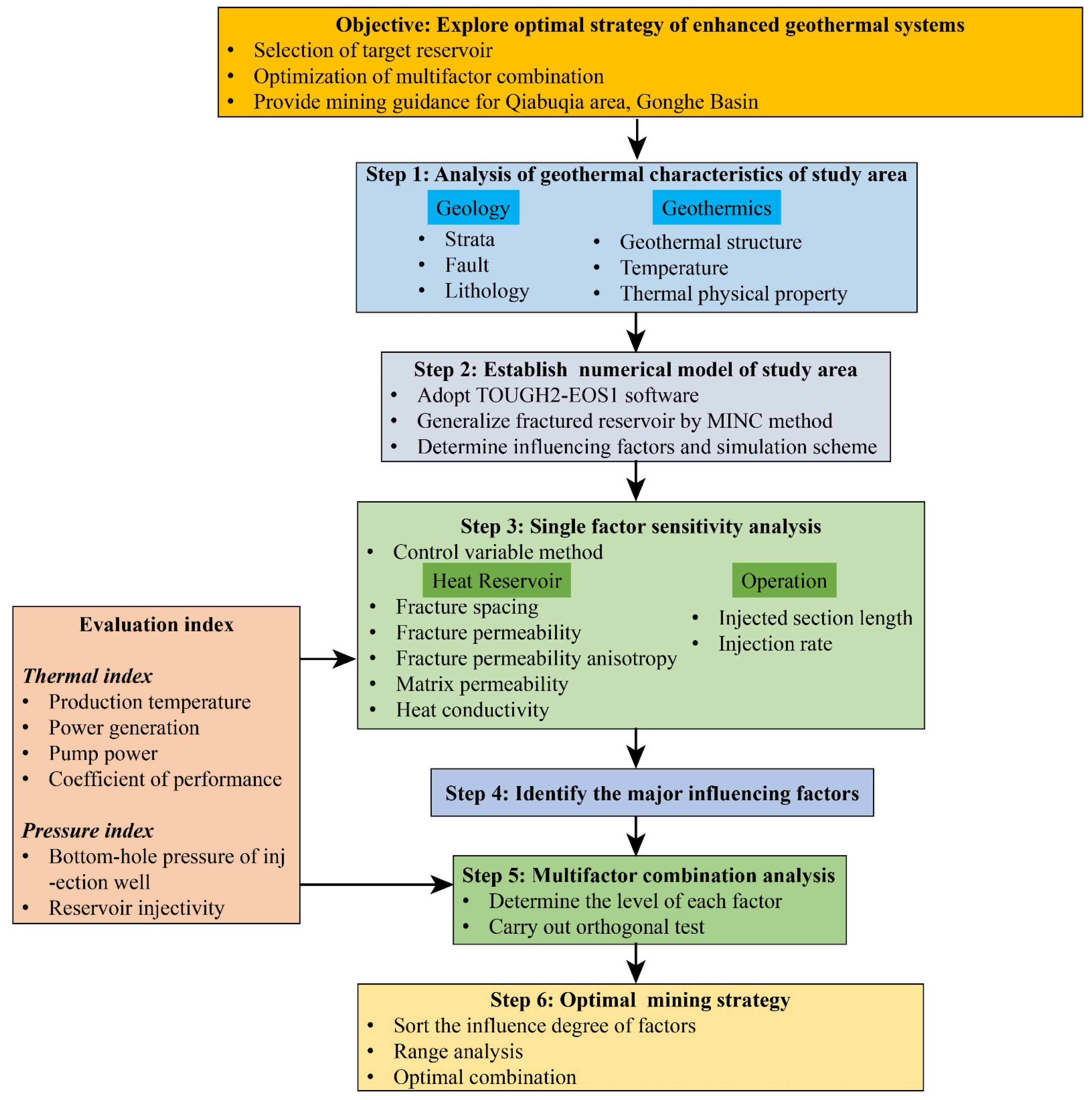
2. Methodology
2.1. Governing Equation of Hydraulic-Thermal Coupled Numerical Model
2.2. Orthogonal Test Method
2.3. Range Analysis
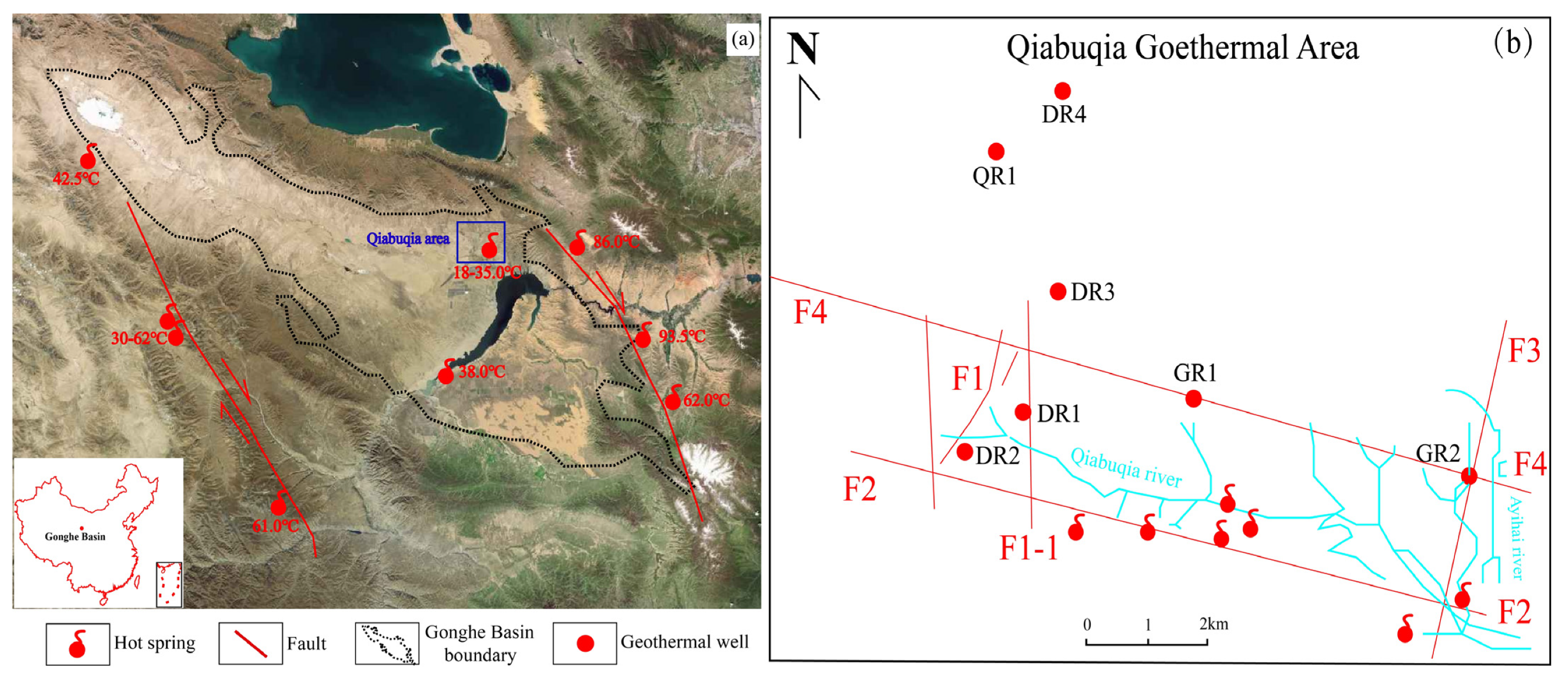
3. Geothermal Characteristics of the Gonghe Basin
3.1. Geological Setting
3.2. Geothermal Features
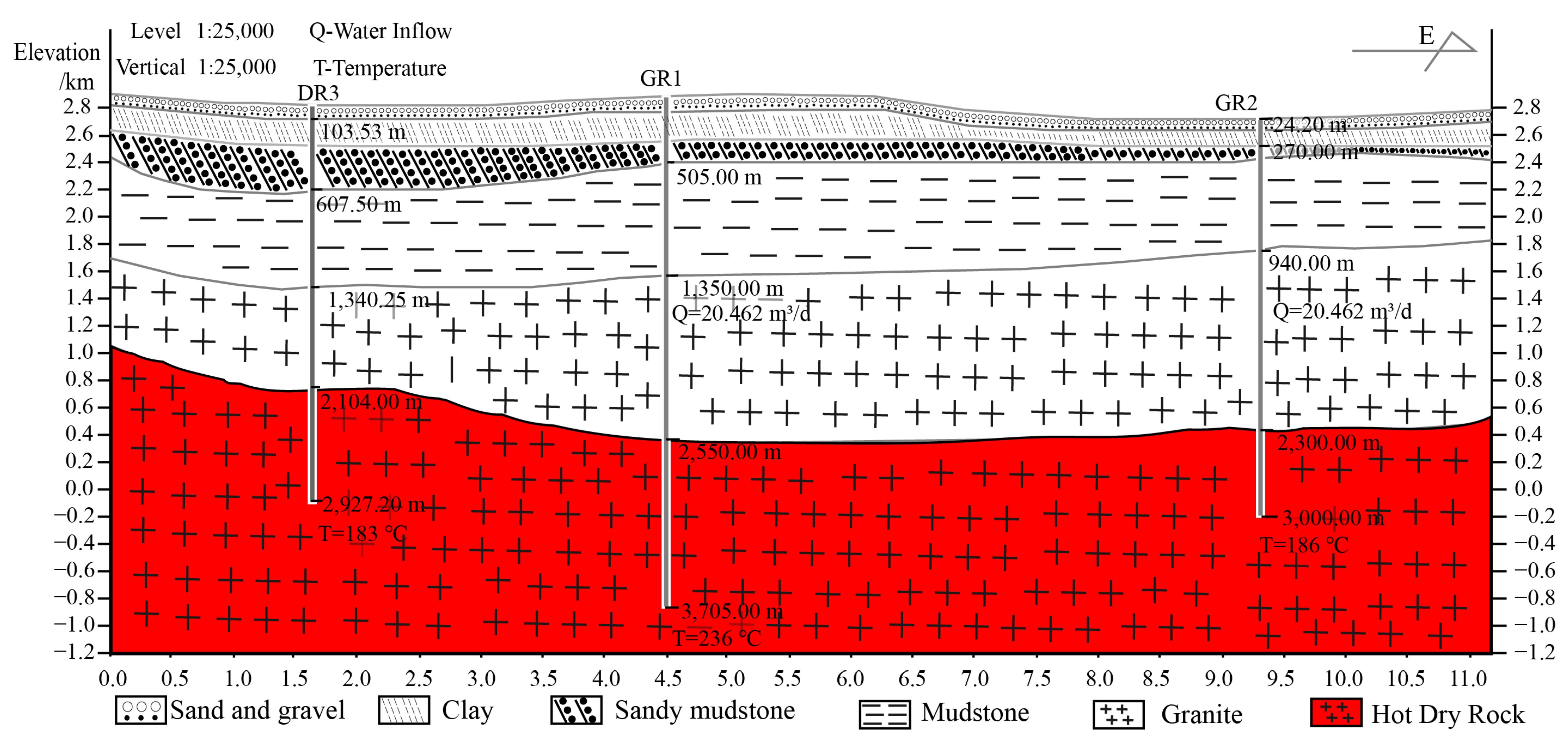
- (1)
- Part I (0~−505 m): The upper of Part I is a thin mid-late Pleistocene sand and gravel layer. Its grain gradually becomes finer downwards; the middle of Part I is mainly the lacustrine deposits of the Gonghe formation. The bottom of Part I is composed of sandy mudstone.
- (2)
- Part II (−505~−1350 m): It is composed of the Linxia formation and the Xianshuihe formation. The lithology is mainly medium-thick mudstone and medium-thick siltstone. The integrity of the mudstone is better. The sandstone particles are finer.
- (3)
- Part III (−1350~−3705 m): It is mid-late Triassic granite; the main lithology is granite and granodiorite. The radioactive heat generation rate of the granite ranges from 1.73 to 4.48 μW/m3, with an average of 3.04 μW/m3, and there is no abnormal high radioactive heat generation rate.
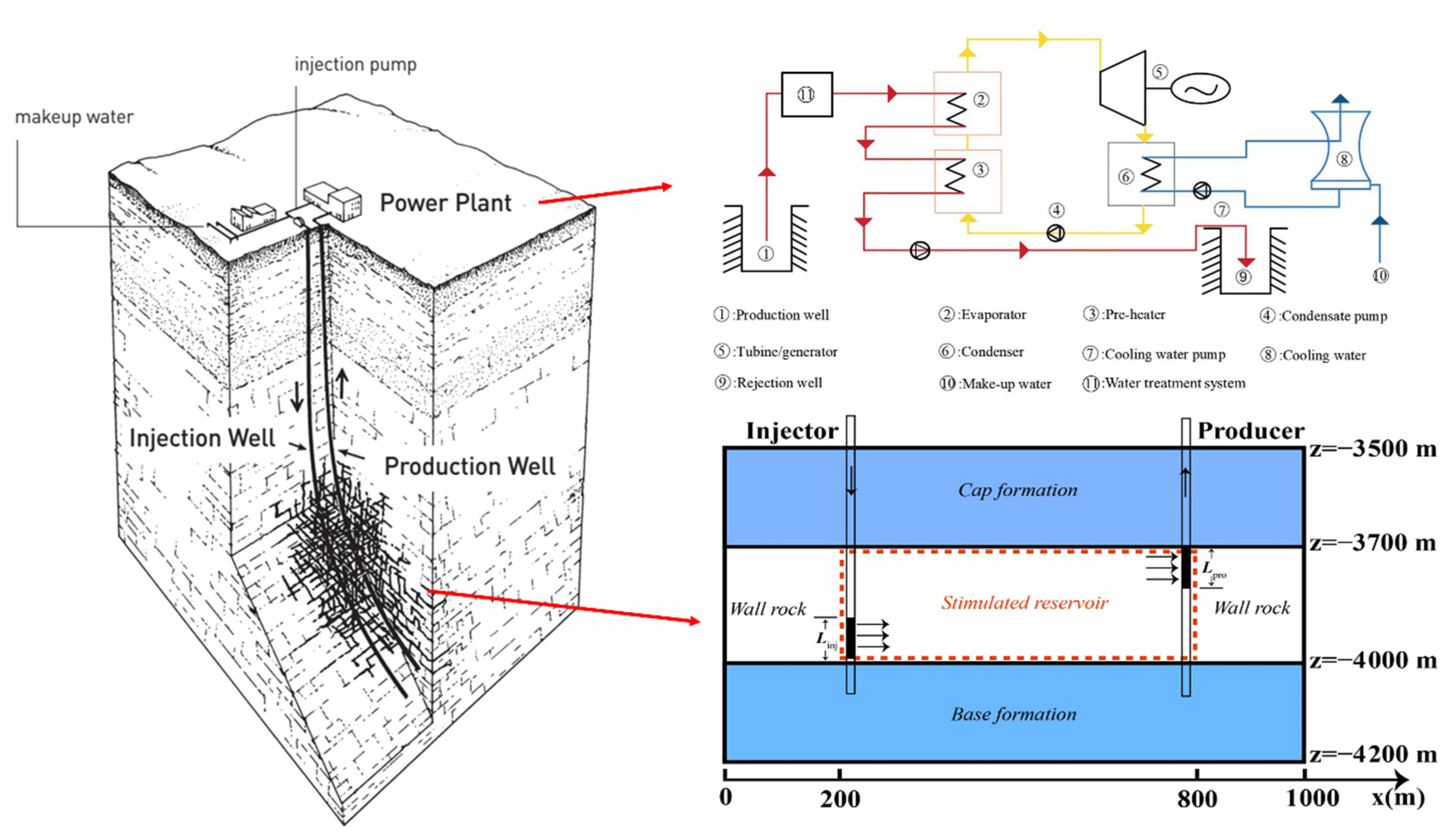
4. EGS Reservoir Production Simulation Analysis
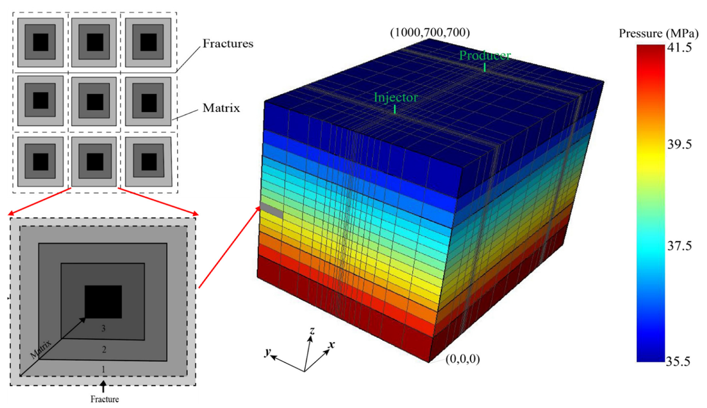
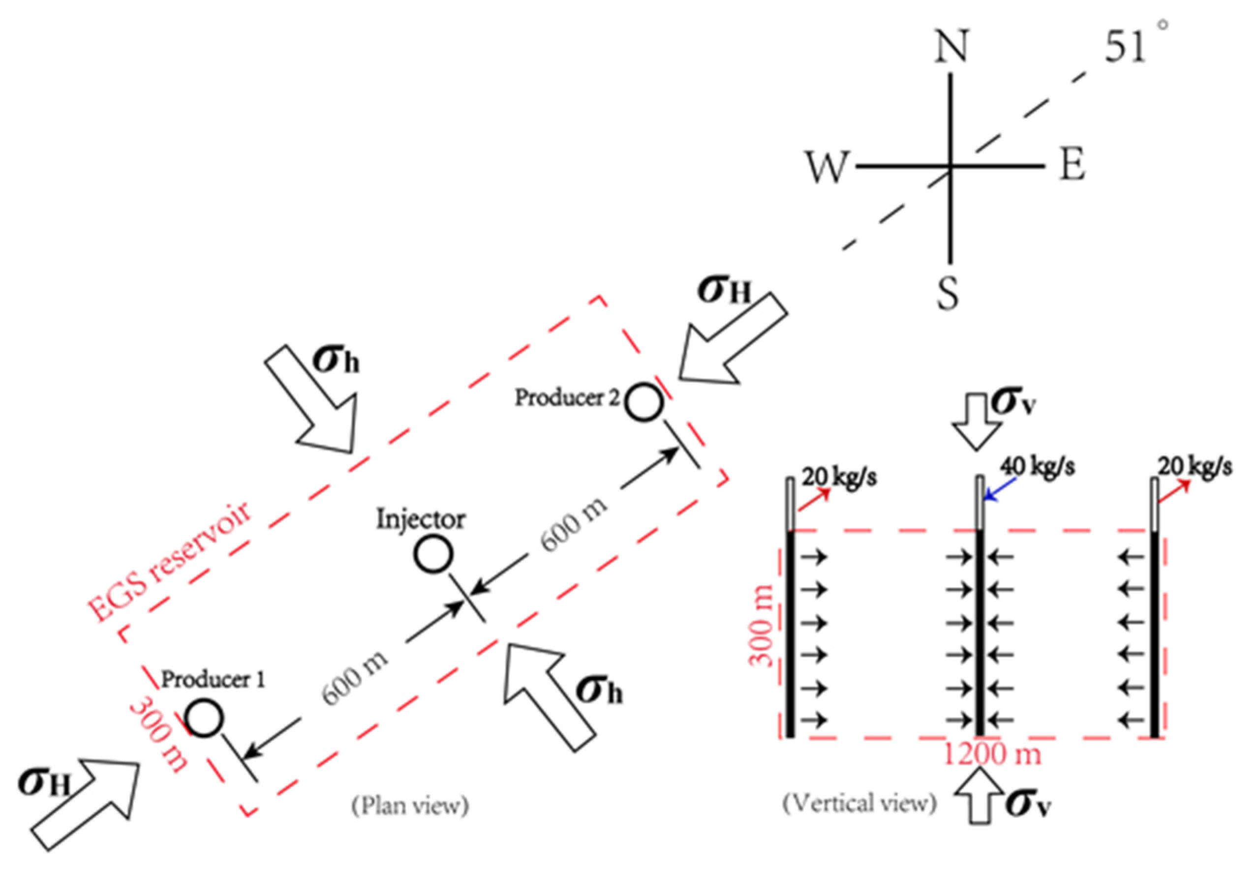
4.1. Target Reservoir and Project Design
4.2. Power System
4.3. Numerical Procedure
4.4. Model Parameters and Single-Factor Sensitivity Scheme
4.5. Initial and Boundary Conditions
4.6. Simulation Results of Single-Factor Sensitivity Analysis
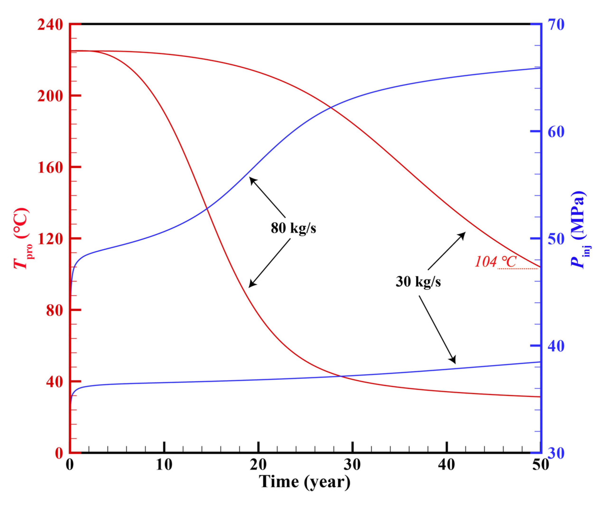
4.6.1. Maximum Injection Rate under Base Case Condition
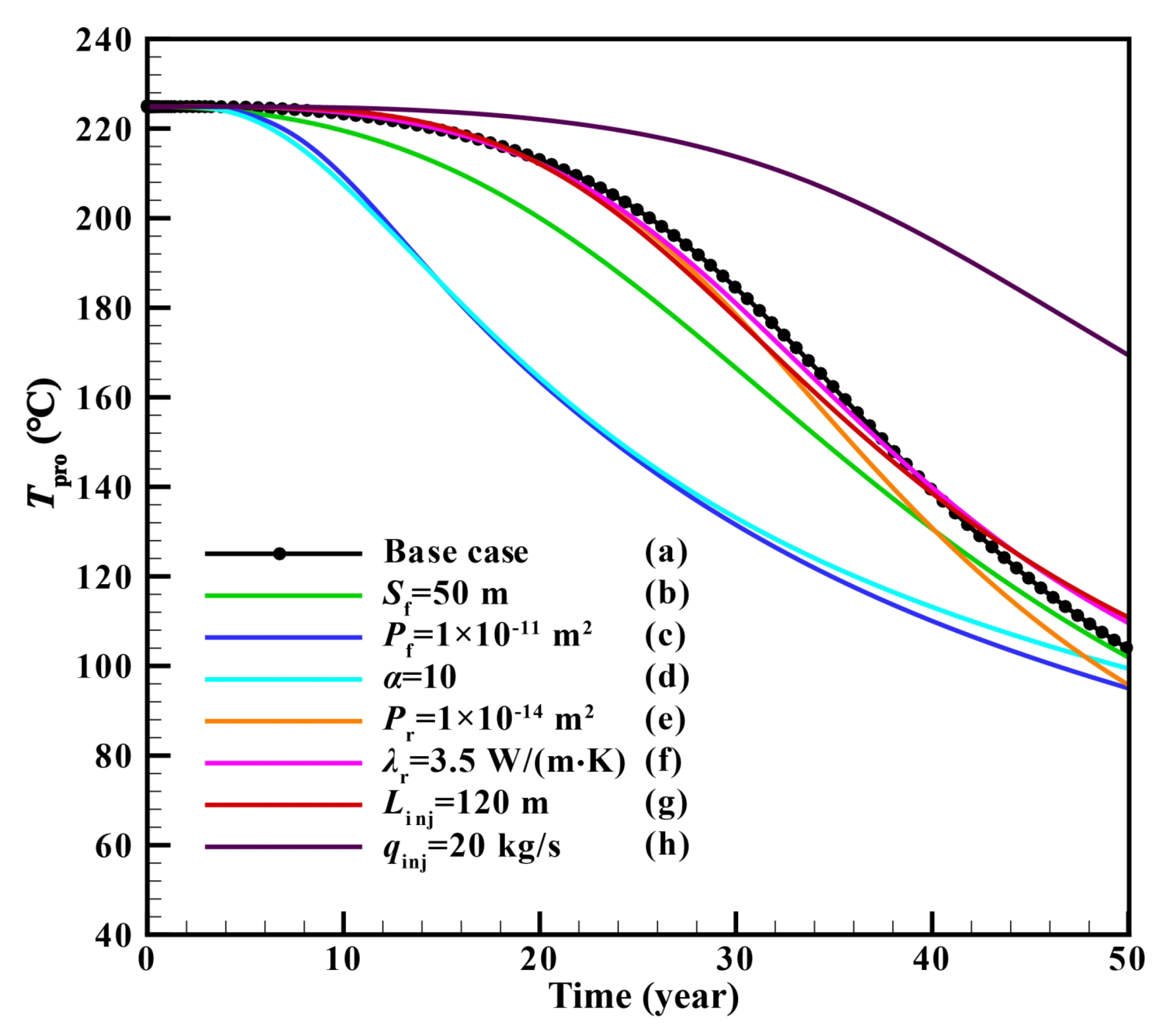
4.6.2. Production Temperature
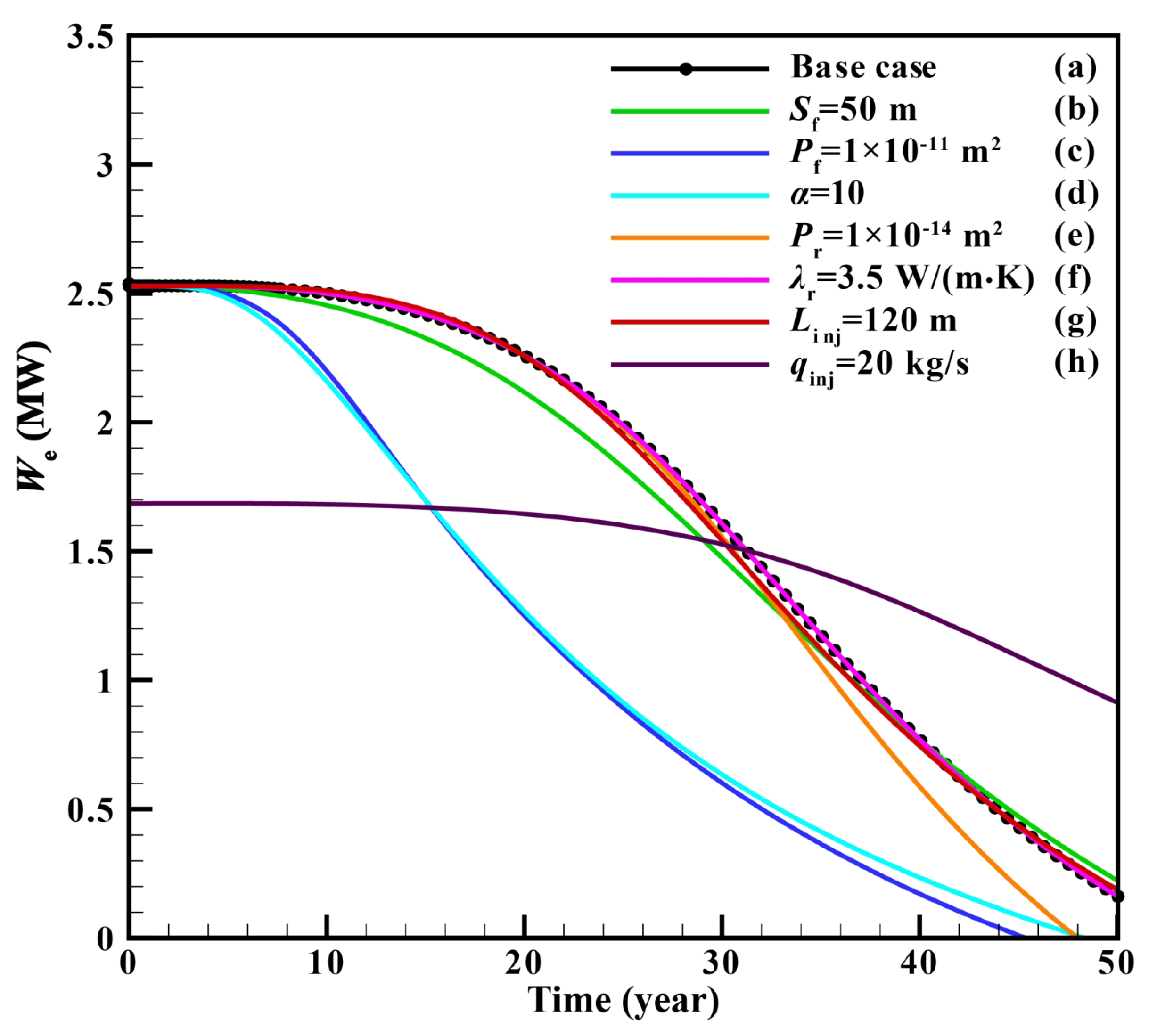
4.6.3. Power Generation
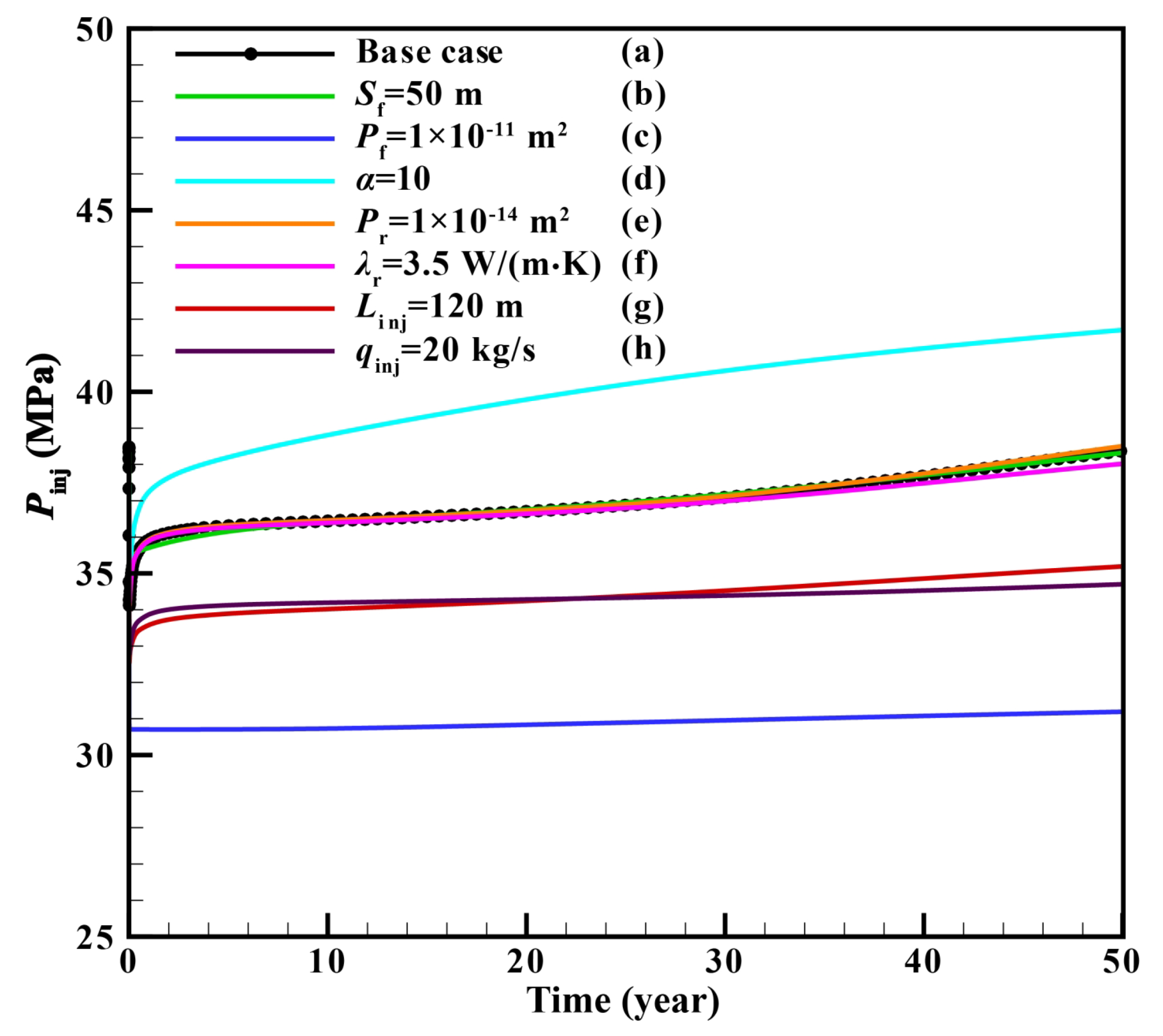
4.6.4. Bottom-Hole Pressure of Injection Well
4.6.5. Reservoir Injectivity
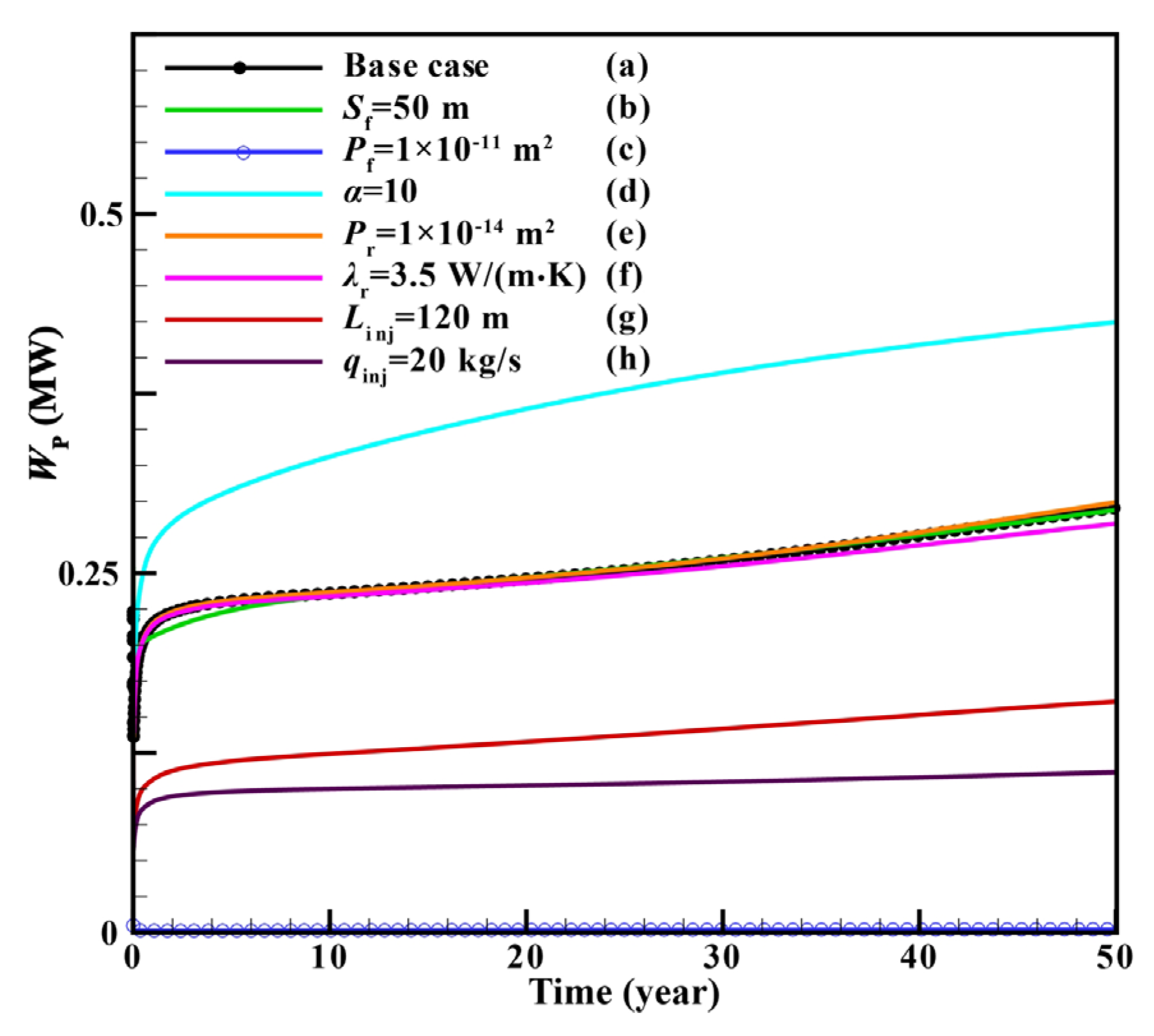
4.6.6. Pump Power
4.6.7. Coefficient of Performance
4.7. Discussions of Single-Factor Sensitivity Analysis
4.7.1. Effect of Reservoir Factors on Production Performance
4.7.2. Effect of Operation Factors on Production Performance
4.7.3. Main Factors Affecting Production Performance
5. Multi-Factor Combination Analysis
5.1. Orthogonal Test Scheme
5.2. Orthogonal Test Results
5.3. Discussions of Multi-Factor Combination Analysis
5.3.1. Effect of Main Factors on Production Performance
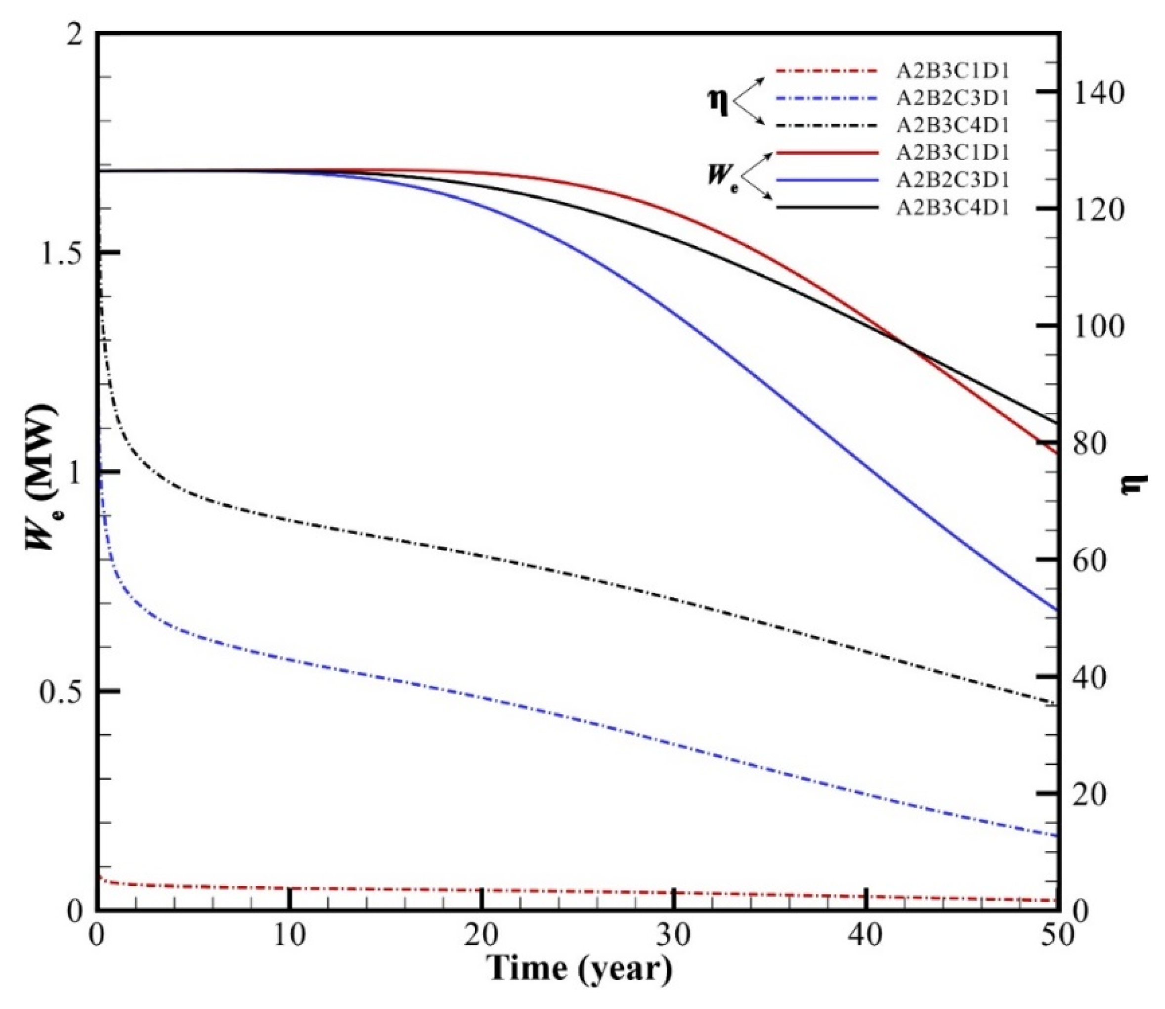
5.3.2. Order of Main Factors and Optimal Combination
5.3.3. Optimal Scheme Considering Fracture Permeability Anisotropy
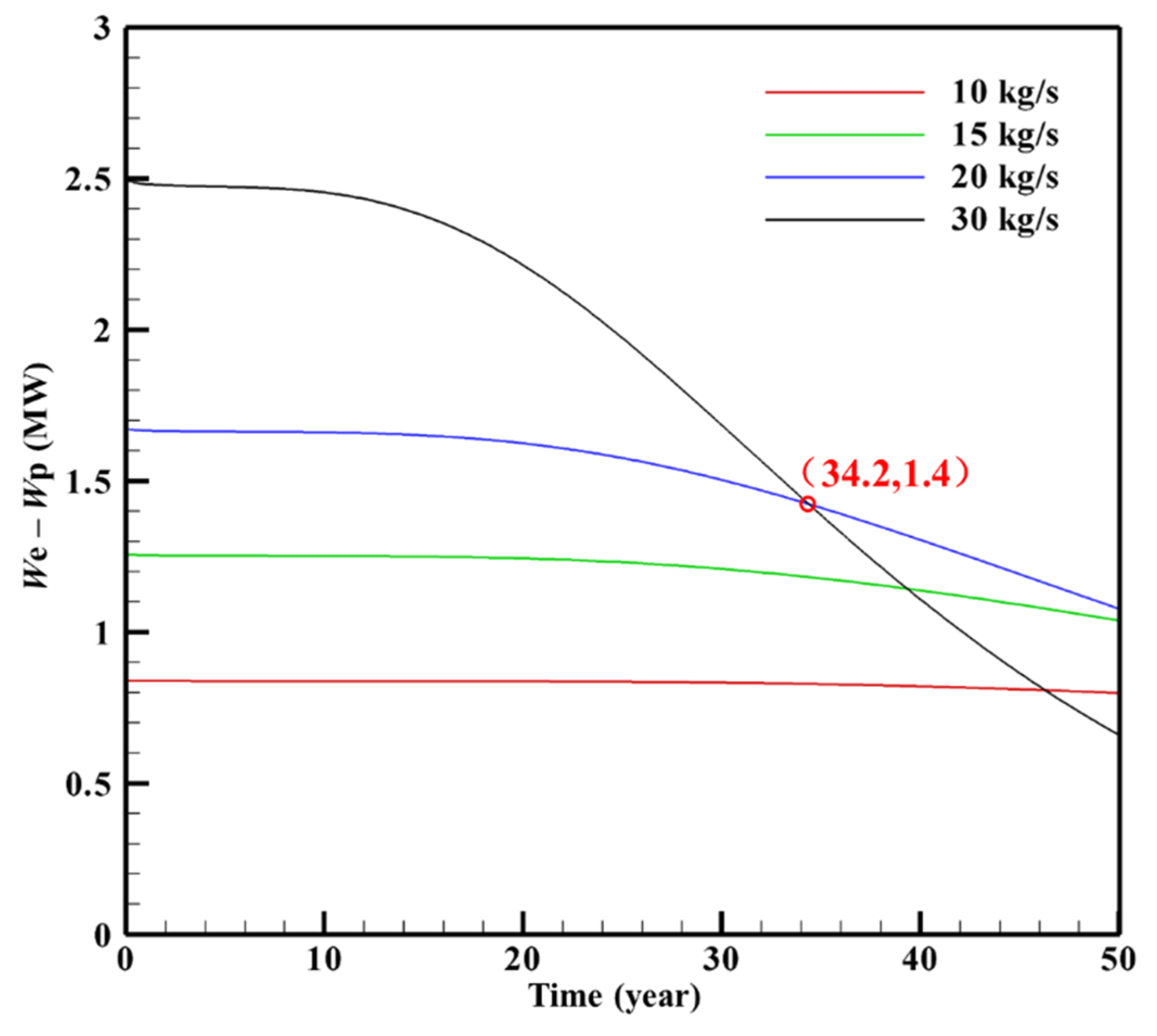
5.3.4. Optimal Scheme Considering Injection Rate
5.3.5. Well Layout Mode
5.3.6. Optimal Scheme Considering Injection Water Temperature
5.3.7. Space Variation of Reservoir Temperature Field
6. Conclusions
- (1)
- The Gonghe Basin possess a good geothermal structure. The molten layer in the depth interval of 15~35 km may be the heat source. The widely distributed huge-thick high-temperature granite formation is an ideal target reservoir for HDR. The cap rocks are mainly mudstone and sandstone, which have the characteristics of low heat conductivity. The complex geological structure has produced many deep large faults, which can serve as heat conduction channels. Therefore, there has formed a relatively shallow high-temperature HDR reservoir in the Gonghe Basin.
- (2)
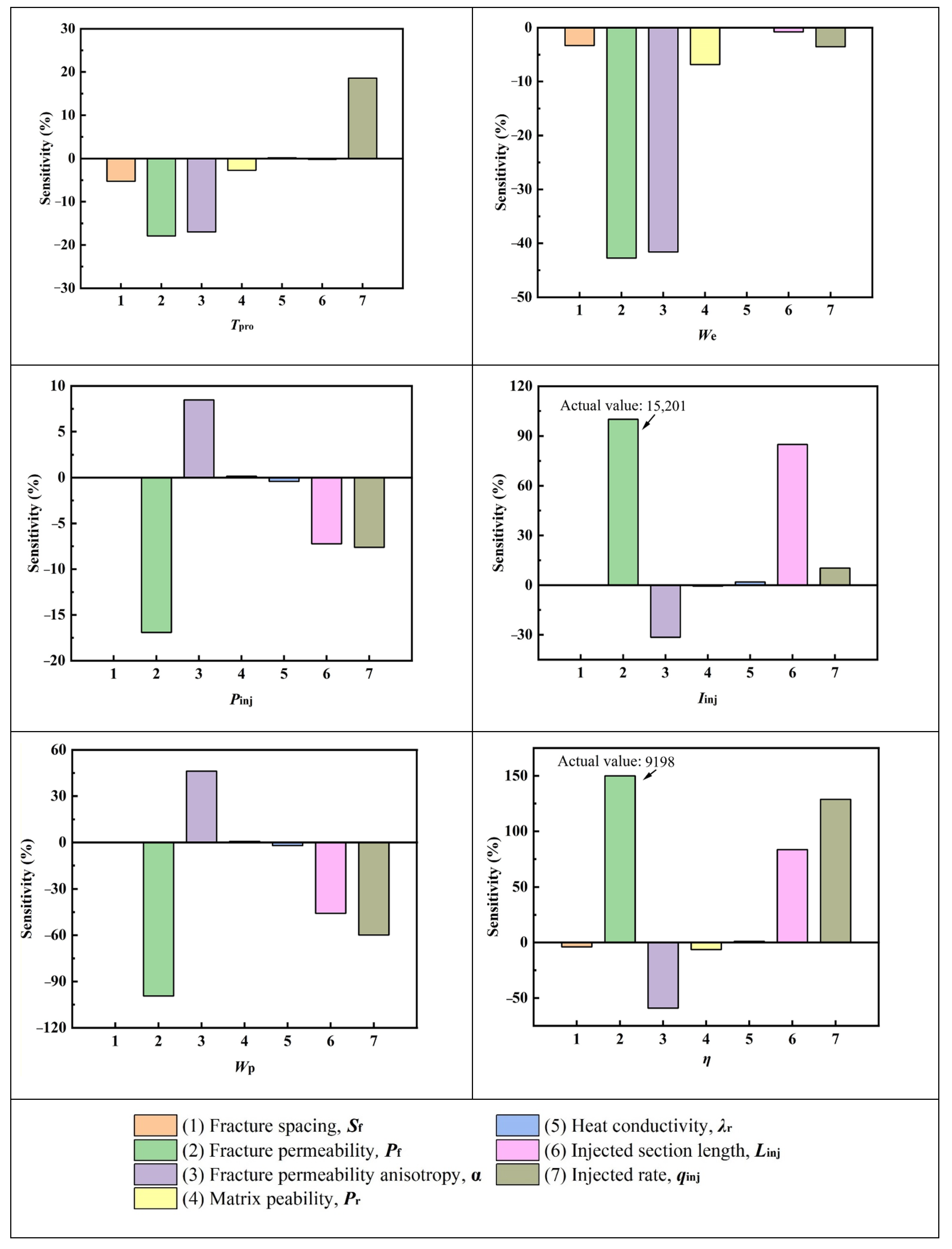
- For single-factor sensitivity analysis, when qinj was constant, the increase of Sf had a slight influence on Tpro and We. Pf had the greatest influence on the production performance among all the factors. For the condition with α = 10, We declined the fastest, while Wp rose the fastest, resulting in the lowest η. The increase of Pr had a slight influence on Tpro and We in the later stage of the project. λr was the least influential of all the parameters. Increasing Linj had little influence on Tpro and We but had great influence on Pinj and Wp. When qinj decreased, the early We decreased due to the flow rate limitation although Tpro declined much more slowly. Meanwhile, Wp decreased and η increased significantly. Therefore, the biggest influence factor on the We value was the overall permeability of the fractured reservoir. For η, Pf was the most important factor, followed by qinj, Linj, and α.
- (3)
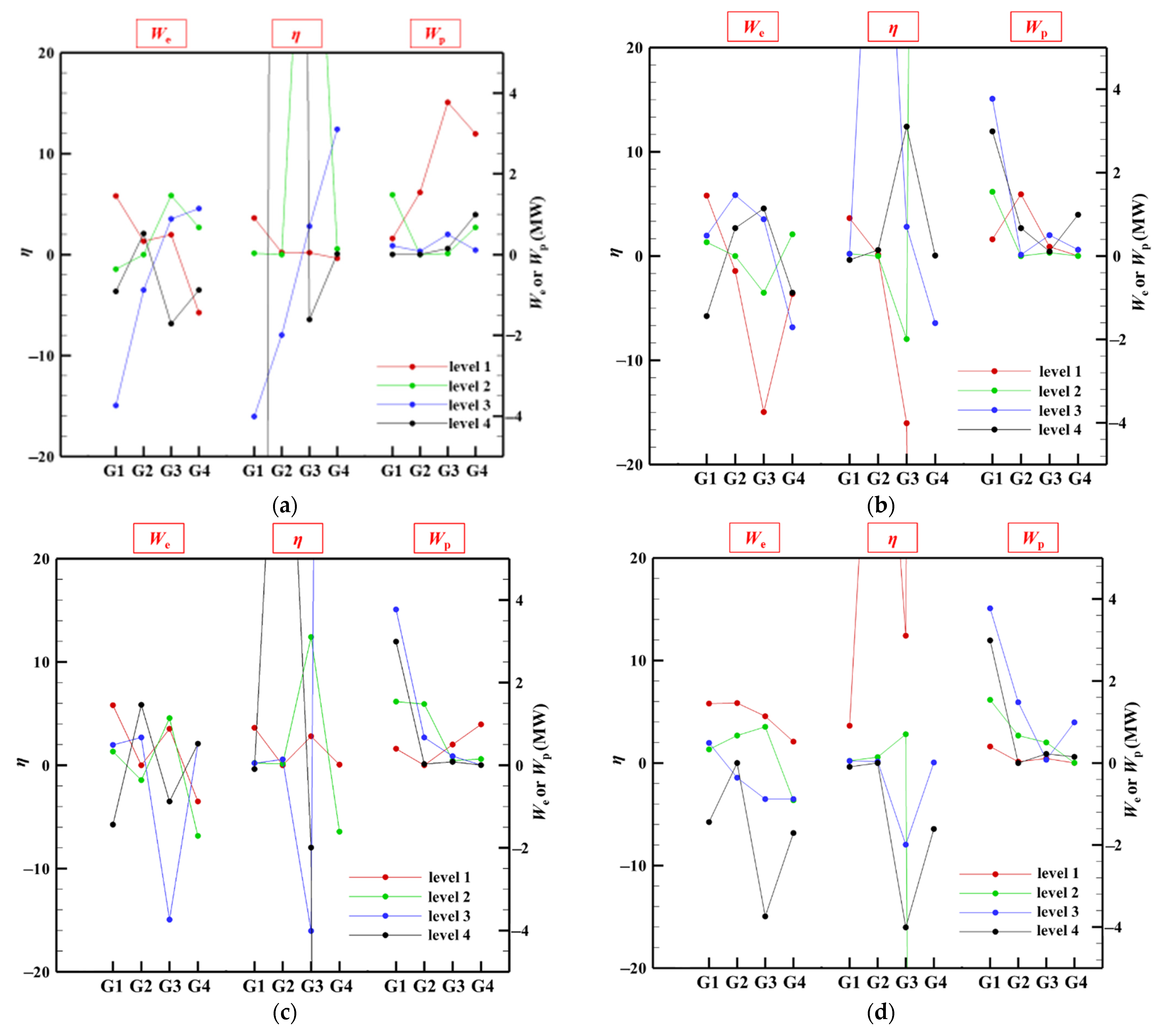
- The four factors of fracture permeability, fracture permeability anisotropy, injected section length, and injection rate had the greatest influence on the EGS production. For the multi-factor sensitivity analysis, the order of influence degree on We was qinj > Pf > α > Linj. The order of influence degree on η was Pf > qinj > Linj > α. On the whole, the rank results of the orthogonal test are almost the same as those of single-factor sensitivity.
- (4)
- Different factor combinations have great influence on the heat transfer performance. The multi-factor and multi-level combination optimization is needed and the optimization scheme of the EGS can be achieved through the orthogonal test and range analysis.
- (5)
- For reservoir stimulation, the stratum with dense natural fractures should be selected as the target EGS reservoir. It is not advisable to acidify the EGS reservoir too much to widen the apertures of natural fractures. This is likely to lead to a rapid decline in net power generation. Fracture permeability anisotropy will increase pump energy consumption, but this adverse effect can be greatly reduced if the other parameters are well matched. Matrix permeability and heat conductivity may not be used as an indicator in selecting a target reservoir.
- (6)
- For project operation, the injected section length should be as long as possible. The injection rate plays a major role in all factors. Special attention should be paid to the value of the injection rate, which should not be too large. The appropriate injection temperature should be determined in accordance with the water source condition and the engineering requirement. If a commercial rate (100 kg/s) is to be obtained, the permeability of the reservoir fracture network needs to be stimulated to be higher. Meanwhile, in order to ensure that the production temperature is both high and stable, it is necessary to further increase the volume of the EGS reservoir.
Author Contributions
Funding
Institutional Review Board Statement
Informed Consent Statement
Data Availability Statement
Conflicts of Interest
Nomenclature
| CR | Rock specific heat, J/(kg·K) | hβ | Specific enthalpy in phase β, J/kg |
| F | Mass or heat flux, kg/m2 or W/m2 | t | Time, s |
| Iinj | Injectivity, kg/s/MPa | uβ | Specific internal energy in phase β, J/kg |
| Linj | Injected section length, m | α | Fracture permeability anisotropy |
| M | Mass or energy per volume, kg/m3 or J/m3 | Φ | Porosity |
| Pf | Fracture permeability, m2 | φ | Sensitivity |
| Pinj | Bottom-hole pressure of injection well, MPa | κ | Mass components |
| Pr | Matrix permeability, m2 | η | Coefficient of performance |
| qinj | Injection rate, kg/s | ηe | Conversion efficiency |
| R | Range | ηp | Pump efficiency |
| Sf | Fracture spacing, m | λr | Heat conductivity, W/(m·K) |
| Sβ | Saturation of phase β | ρR | Rock density, kg/m3 |
| T | Temperature, °C | ρβ | Density of phase β, kg/m3 |
| Tpro | Production water temperature, °C | vβ | Darcy velocity in phase β, m/s |
| Vn | Subdomain of the flow system | μβ | Dynamic coefficient of viscosity, Pa·s |
| We | Power generation, MW | σH | Maximum horizontal stress, MPa |
| Wp | Pump power, MW | σV | Vertical principal stress, MPa |
| z | Depth, m | σh | Minimum horizontal stress, MPa |
References
- Tester, J.; Livesay, B.; Anderson, B.; Moore, M.; Bathchelor, A.; Nichols, K.; Blackwell, D.; Petty, S.; DiPippo, D.; Toksoz, M.; et al. The Future of Geothermal Energy: Impact of Enhanced Geothermal Systems (EGS) on the United States in the 21st Century; An Assessment by an MIT-Led Interdisciplinary Panel; Massachusetts Institute of Technology: Cambridge, MA, USA, 2006. [Google Scholar]
- Li, S.; Wang, S.; Tang, H. Stimulation mechanism and design of enhanced geothermal systems: A comprehensive review. Renew. Sustain. Energy Rev. 2022, 155, 111914. [Google Scholar] [CrossRef]
- Wang, J.; Hu, S.; Pang, Z.; He, L.; Zhao, P.; Zhu, C.; Rao, S.; Tang, X.; Kong, Y.; Luo, L.; et al. Estimate of geothermal resources potential for hot dry rock in the continental area of China. Sci. Technol. Rev. 2012, 30, 25–31. (In Chinese) [Google Scholar]
- Zhang, Y.; Zhang, Y.J.; Zhou, L.; Lei, Z.H.; Guo, L.L.; Zhou, J. Reservoir stimulation design and evaluation of heat exploitation of a two-horizontal-well enhanced geothermal system (EGS) in the Zhacang geothermal field, Northwest China. Renew. Energy 2022, 183, 330–350. [Google Scholar] [CrossRef]
- Hofmann, H.; Babadagli, T.; Zimmermann, G. Hot water generation for oil sands processing from enhanced geothermal systems: Process simulation for different hydraulic fracturing scenarios. Appl. Energy 2016, 113, 524–547. [Google Scholar] [CrossRef]
- Barenblatt, G.; Zheltov, I.; Kochina, I. Basic concepts in the theory of seepage of homogeneous liquids in fissured rocks. J. Appl. Math. Mech. 1960, 24, 1286–1303. [Google Scholar] [CrossRef]
- Warren, J.E.; Root, J.P. The Behavior of Naturally Fractured Reservoirs. Soc. Pet. Eng. J. 1963, 228, 245–255. [Google Scholar] [CrossRef] [Green Version]
- Zeng, Y.; Su, C.Z.; Wu, N.Y. Numerical simulation of heat production potential from hot dry rock by water circulating through two horizontal wells at Desert Peak geothermal field. Energy 2013, 10, 92–107. [Google Scholar] [CrossRef]
- Suzuki, A.; Fomin, S.A.; Chugunov, V.A.; Niibori, Y.; Hashida, T. Fractional diffusion modeling of heat transfer in porous and fractured media. Int. J. Heat Mass Transf. 2016, 103, 611–618. [Google Scholar] [CrossRef]
- Gong, F.; Guo, T.; Sun, W.; Li, Z.; Yang, B.; Chen, Y.; Qu, Z. Evaluation of geothermal energy extraction in Enhanced Geothermal System (EGS) with multiple fracturing horizontal wells (MFHW). Renew. Energy 2020, 151, 1339–1351. [Google Scholar] [CrossRef]
- Zhou, D.J.; Tatomir, A.; Niemi, A.; Tang, C.F.; Sauter, M. Study on the influence of randomly distributed fracture aperture in a fracture network on heat production from an enhanced geothermal system (EGS). Energy 2022, 250, 123–781. [Google Scholar] [CrossRef]
- Pandey, S.N.; Chaudhuri, A.; Kelkar, S. A coupled thermo-hydro-mechanical modeling of fracture aperture alteration and reservoir deformation during heat extraction from a geothermal reservoir. Geothermics 2017, 65, 17–31. [Google Scholar] [CrossRef]
- Soltani, M.; Kashkooli, F.M.; Souri, M.; Rafiei, B.; Jabarifar, M.; Gharali, K.; Nathwani, J.S. Environmental, economic, and social impacts of geothermal energy systems. Renew. Sustain. Energy Rev. 2021, 140, 110–750. [Google Scholar] [CrossRef]
- Guo, T.; Gong, F.; Wang, X.; Lin, Q.; Qu, Z.; Zhang, W. Performance of enhanced geothermal system (EGS) in fractured geothermal reservoirs with CO2 as working fluid. Appl. Eng. 2019, 152, 215–230. [Google Scholar] [CrossRef]
- Huang, W. Heat extraction performance of EGS with heterogeneous reservoir: A numerical evaluation. Int. J. Heat Mass Transf. 2017, 13, 645–657. [Google Scholar] [CrossRef] [Green Version]
- Guo, B.; Fu, P.; Hao, Y.; Peters, C.A.; Carrigan, C.R. Thermal drawdown-induced flow channeling in a single fracture in EGS. Geothermics 2016, 61, 46–62. [Google Scholar] [CrossRef] [Green Version]
- Asai, P.; Panja, P.; McLennan, J.; Deo, M. Effect of different flow schemes on heat recovery from Enhanced Geotherm al Systems (EGS). Energy 2019, 175, 667–676. [Google Scholar] [CrossRef]
- Patterson, J.R.; Cardiff, M.; Feig, K.L. Optimizing geothermal production in fractured rock reservoirs under uncertainty. Geothermics 2020, 88, 101–906. [Google Scholar] [CrossRef]
- Wu, X.T.; Li, Y.C.; Tang, C.A. Fracture spacing in horizontal well multi-perforation fracturing optimized by heat extraction. Geothermics 2022, 101, 102–376. [Google Scholar] [CrossRef]
- Fisher, A. A mathematic examination of the methods of determining the accuracy of an observation by the mean error and by the mean square error. Mon. Not. R Astron. Soc. 1920, 80, 758–770. [Google Scholar] [CrossRef] [Green Version]
- Han, Y.S.; He, J.T.; Lu, Y.T. Sensitivity of the properties of the graduated compression stocking and soft tissues on the lower limb-stocking interfacial pressure using the orthogonal simulation test. Med. Eng. Phys. 2021, 95, 84–89. [Google Scholar] [CrossRef]
- Lin, R.; Diao, X.Y.; Ma, T.C.; Tang, S.H.; Chen, L.; Liu, D.C. Optimized microporous layer for improving polymer exchange membrane fuel cell performance using orthogonal test design. Appl. Energy 2019, 254, 113–714. [Google Scholar] [CrossRef]
- Xie, J.X.; Wang, J.S. Performance optimization of pinnate horizontal well in geothermal energy utilization with orthogonal test. Appl. Therm. Eng. 2022, 209, 118–321. [Google Scholar] [CrossRef]
- Yu, L.K.; Wu, X.T.; Hassan, N.S.; Wang, Y.D.; Ma, W.W.; Liu, G. Modified zipper fracturing in enhance d geothermal system reservoir and analyzed heat extraction optimization via orthogonal design. Renew. Energy 2020, 161, 373–385. [Google Scholar] [CrossRef]
- Pruess, K.; Oldenburg, C.; Moridis, G. TOUGH2 User’s Guide, Version 2.0; Lawrence Berkeley National Laboratory: Berkeley, CA, USA, 1999. [Google Scholar]
- Pruess, K.; Faybishenho, B.; Bodvarsson, G.S. Alternative concepts and approaches for modeling flow and transport in thick unsaturated zones of fractured rocks. J. Contam. Hydrol. 1999, 38, 281–322. [Google Scholar] [CrossRef]
- Wu, L.; Liu, J.; Zhou, J.; Zhang, Q.; Song, Y.; Du, S.; Tian, W. Evaluation of tar from the microwave co-pyrolysis of low-rank coal and corncob using orthogonal-test-based grey relational analysis (GRA). J. Clean. Prod. 2022, 337, 130–362. [Google Scholar] [CrossRef]
- Gao, J.; Zhang, H.J.; Zhang, S.Q.; Chen, X.B.; Cheng, Z.P.; Jia, X.F. Three-dimensional magnetotelluric imaging of the geothermal system beneath the Gonghe Basin, Northeast Tibetan Plateau. Geothermics 2018, 76, 15–25. [Google Scholar] [CrossRef]
- Zhang, C.; Jiang, G.; Shi, Y.; Wang, Z.; Wang, Y.; Li, S.; Jia, X.; Hu, S. Terrestrial heat flow and crustal thermal structure of the Gonghe-Guide area, northeastern Qinghai-Tibetan plateau. Geothermics 2018, 72, 182–192. [Google Scholar] [CrossRef]
- Zhang, S.Q.; Li, X.F.; Song, J.; Wen, D.G.; Li, Z.W.; Li, D.M.; Cheng, Z.; Fu, L.; Zhang, L.; Feng, Q.; et al. Analysis on Geophysical Evidence for Existence of Partial Melting Layer in Crust and Regional Heat Source Mechanism for Hot Dry Rock Resources of Gonghe Basin. Earth Sci. 2021, 46, 1416–1436. [Google Scholar]
- Genter, A.; Fritsch, D.; Cuenot, N.; Baumgärtner, J.; Graff, J.J. Overview of the current activities of the European EGS Soultz project: From exploration to electricity production. In Proceedings of the Thirty-Fourth Workshop on Geothermal Reservoir Engineering Stanford University, Stanford, CA, USA, 9–11 February 2009. SGP-TR-187. [Google Scholar]
- U.S. Department of Energy. Geothermal Technologies Program 2013 Peer Review; U.S. Department of Energy: Washington, DC, USA, 2013.
- Lei, Z.H.; Zhang, Y.J. Investigation on the effect of symmetrical multi-well layout on geothermal energy extraction from a fractured granitic reservoir: A case study in the Gonghe Basin, Northwestern China. Energy Rep. 2021, 7, 7741–7758. [Google Scholar] [CrossRef]
- Huang, X.X.; Zhu, J.L.; Niu, C.K.; Li, J.; Hu, X.; Jin, X.P. Heat extraction and power production forecast of a prospective enhanced geothermal system site in Songliao Basin. China Energy 2014, 75, 360–370. [Google Scholar] [CrossRef]
- Zhang, Y.J.; Li, Z.W.; Yu, Z.W.; Guo, L.L.; Jin, X.P.; Xu, T.F. Evaluation of developing an enhanced geothermal heating system in northeast China: Field hydraulic stimulation and heat production forecast. Energy Build. 2015, 88, 1–14. [Google Scholar] [CrossRef]
- Zoback, M.D. Reservoir Geomechanics, 1st ed.; Cambridge University Press: Cambridge, UK; New York, NY, USA, 2007; p. 464. [Google Scholar]
- Hofmann, H.; Weides, S.; Babadagli, T.; Zimmermann, G.; Moeck, I.; Majorowicz, J.; Unsworth, M. Potential for enhanced geothermal systems in Alberta, Canada. Energy 2014, 69, 578–591. [Google Scholar] [CrossRef]
- Garg, S.K.; Combs, J. A reformulation of USGS volumetric “heat in place” resource heat in place” resource estimation method. Geothermics 2015, 55, 150–158. [Google Scholar] [CrossRef]
- NIST. Thermophysical Properties of Fluid Systems. 2010. Available online: http://webbook.nist.gov/chemistry/fluid/ (accessed on 1 January 2022).
- Guo, L.L.; Zhang, Y.B.; Zhang, Y.J.; Yu, Z.W.; Zhang, J.N. Experimental investigation of granite properties under different temperatures and pressures and numerical analysis of damage effect in enhanced geothermal system. Renew. Energy 2018, 126, 107–125. [Google Scholar] [CrossRef]
- Li, Z.W.; Feng, X.T.; Zhang, Y.J.; Xu, T.F. Feasibility study of developing a geothermal heating system in naturally fractured formations: Reservoir hydraulic properties determination and heat production forecast. Geothermics 2018, 73, 1–15. [Google Scholar] [CrossRef]
- Cheng, W.L.; Wang, C.L.; Nian, Y.L.; Han, B.B.; Liu, J. Analysis of influencing factors of heat extraction from enhanced geothermal systems considering water losses. Energy 2016, 115, 274–288. [Google Scholar] [CrossRef]
- Sanyal, S.K.; Butler, S.J. An analysis of power generation prospects from enhanced geothermal systems. In Proceedings of theWorld Geothermal Congress, Antalya, Turkey, 24–29 April 2005; pp. 1–6. [Google Scholar]


| Level | Factor | ||
|---|---|---|---|
| A | B | C | |
| Level l | a1 | b1 | c1 |
| Level 2 | a2 | b2 | c2 |
| Level 3 | a3 | b3 | c3 |
| Test Number | Factor | ||
|---|---|---|---|
| A | B | C | |
| 1 | a1 | b1 | c1 |
| 2 | a1 | b2 | c2 |
| 3 | a1 | b3 | c3 |
| 4 | a2 | b1 | c3 |
| 5 | a2 | b2 | c1 |
| 6 | a2 | b3 | c2 |
| 7 | a3 | b1 | c2 |
| 8 | a3 | b2 | c3 |
| 9 | a3 | b3 | c1 |
| Wells | Depth, z (km) | Measured Temperature, T (°C) |
|---|---|---|
| GR1 | 0.1~1.0 | T = 66.061z + 18.467 (R2 = 0.9958) |
| 1.1~2.8 | T = 40.289z + 48.992 (R2 = 0.9967) | |
| 2.9~3.6 | T = 57.738z − 5.0238 (R2 = 0.9861) | |
| GR2 | 0.1~3.0 | T = 50.154z + 33.795 (R2 = 0.9996) |
| DR3 | 0.1~1.4 | T = 72.879z + 14.198 (R2 = 0.9988) |
| 1.5~2.9 | T = 44.357z + 55.081 (R2 = 0.996) | |
| DR4 | 0.1~0.5 | T = 7z + 77.3 (R2 = 0.9423) |
| 0.6~1.5 | T = 8.303z + 99.782 (R2 = 0.91) | |
| 1.6~3.1 | T = 44.456z + 46.466 (R2 = 0.9983) |
| Lithology | Depth (km) | Heat Conductivity (W/(m·K)) |
|---|---|---|
| Mudstone | 0.20~1.40 | 1.25~1.99 (average is 1.58) |
| Igneous Rock | 1.50–3.63 | 2.10–3.17 (average is 2.53) |
| Items | Parameters | Base Case Value | Selected Case Value |
|---|---|---|---|
| Reservoir | Fracture spacing, Sf | 3 m | 50 m |
| Fracture permeability (kx = ky = kz), Pf | 1 × 10⁻¹³ m2 | 1 × 10⁻¹¹ m2 | |
| Fracture permeability anisotropy, α (α = kx/kz, kx = ky), | 1 | 10 | |
| Matrix permeability, Pr | 1 × 10⁻¹⁷ m2 | 1 × 10⁻¹⁴ m2 | |
| Matrix porosity | 0.025 | No changed | |
| Matrix density | 2360 kg/m3 | No changed | |
| Heat conductivity, λr | 2.0 W/(m·K) | 3.5 W/(m·K) | |
| Specific heat | 754.4 J/(kg·K) | No changed | |
| Initial pressure | P = 4 × 10⁻⁷–10,000z (Pa) | No changed | |
| Initial temperature | 225 °C | No changed | |
| Operation | Injected section length, Linj | 60 m | 120 m |
| Injection rate, qinj | 30 kg/s | 20 kg/s | |
| Injection water temperature | 10 °C | No changed | |
| Injection water specific enthalpy | 78.77 kJ/kg | No changed | |
| Productivity index | 5.4 × 10⁻¹² m3 | No changed | |
| Production bottom-hole pressure | 30 MPa | No changed |
| Level | Factors | |||
|---|---|---|---|---|
| A | B | C | D | |
| Fracture Permeability, Pf (m2) | Fracture Permeability Anisotropy, α | Injected Section Length, Linj (m) | Injection Rate, qinj (kg/s) | |
| 1 | 5 × 10⁻¹⁴ | 1 | 30 | 20 |
| 2 | 1 × 10⁻¹³ | 10 | 120 | 50 |
| 3 | 1 × 10⁻¹² | 100 | 210 | 80 |
| 4 | 1 × 10⁻¹¹ | 1000 | 300 | 110 |
| Test Number | Factors | |||
|---|---|---|---|---|
| A | B | C | D | |
| Fracture Permeability, Pf (m2) | Fracture Permeability Anisotropy, α | Injected Section Length, Linj (m) | Injection Rate, qinj (kg/s) | |
| 1 | A1 (5 × 10⁻¹⁴) | B1 (1) | C1 (30) | D1 (20) |
| 2 | A1 (5 × 10⁻¹⁴) | B2 (10) | C2 (120) | D2 (50) |
| 3 | A1 (5 × 10⁻¹⁴) | B3 (100) | C3 (210) | D3 (80) |
| 4 | A1 (5 × 10⁻¹⁴) | B4 (1000) | C4 (300) | D4 (110) |
| 5 | A2 (1 × 10⁻¹³) | B1 (1) | C2 (120) | D3 (80) |
| 6 | A2 (1 × 10⁻¹³) | B2 (10) | C1 (30) | D4 (110) |
| 7 | A2 (1 × 10⁻¹³) | B3 (100) | C4 (300) | D1 (20) |
| 8 | A2 (1 × 10⁻¹³) | B4 (1000) | C3 (210) | D2 (50) |
| 9 | A3 (1 × 10⁻¹²) | B1 (1) | C3 (210) | D4 (110) |
| 10 | A3 (1 × 10⁻¹²) | B2 (10) | C4 (300) | D3 (80) |
| 11 | A3 (1 × 10⁻¹²) | B3 (100) | C1 (30) | D2 (50) |
| 12 | A3 (1 × 10⁻¹²) | B4 (1000) | C2 (120) | D1 (20) |
| 13 | A4 (1 × 10⁻¹¹) | B1 (1) | C4 (300) | D2 (50) |
| 14 | A4 (1 × 10⁻¹¹) | B2 (10) | C3 (210) | D1 (20) |
| 15 | A4 (1 × 10⁻¹¹) | B3 (100) | C2 (120) | D4 (110) |
| 16 | A4 (1 × 10⁻¹¹) | B4 (1000) | C1 (30) | D3 (80) |
| Test Number | Index | ||||||
|---|---|---|---|---|---|---|---|
| Power Generation, We | Coefficient of Performance, η | Production Temperature, Tpro | Injectivity, Iinj | Bottom-Hole Pressure, Pinj | Pump Power, Wp | ||
| 1 | VEnd VAve. | 1.00 1.45 | 2.38 3.63 | 176.46 208.11 | 1.13 1.17 | 30.69 30.61 | 0.42 0.40 |
| 2 | VEnd VAve. | −1.60 0.33 | −0.88 0.21 | 52.87 110.62 | 1.79 2.12 | 60.27 55.82 | 1.81 1.54 |
| 3 | VEnd VAve. | −1.24 0.49 | −0.28 0.20 | 77.53 110.07 | 1.96 2.32 | 74.69 68.63 | 4.38 3.77 |
| 4 | VEnd VAve. | −3.35 −1.44 | −1.01 −0.37 | 54.78 81.09 | 5.01 5.62 | 55.83 53.46 | 3.30 2.99 |
| 5 | VEnd VAve. | −2.62 −0.36 | −1.55 0.13 | 51.67 93.97 | 4.68 5.42 | 49.62 46.90 | 1.69 1.48 |
| 6 | VEnd VAve. | - | - | - | - | - | - |
| 7 | VEnd VAve. | 1.11 1.46 | 35.26 51.99 | 183.40 208.79 | 17.43 19.28 | 33.65 33.44 | 0.03 0.03 |
| 8 | VEnd VAve. | −0.86 0.67 | −0.31 0.57 | 222.41 223.83 | 1.22 1.69 | 74.70 64.89 | −0.86 0.67 |
| 9 | VEnd VAve. | −4.96 −3.74 | −20.56 −16.04 | 32.41 49.37 | 45.66 48.45 | 36.71 36.00 | 0.24 0.22 |
| 10 | VEnd VAve. | −2.29 -0.88 | −24.98 −7.97 | 57.69 84.32 | 95.71 110.12 | 34.60 34.12 | 0.09 0.08 |
| 11 | VEnd VAve. | −1.27 0.88 | −2.08 2.80 | 62.2 126.6 | 4.39 5.15 | 45.92 42.59 | 0.61 0.50 |
| 12 | VEnd VAve. | 0.43 1.14 | 5.55 12.41 | 132.38 185.98 | 2.65 3.63 | 38.82 36.93 | 0.16 0.11 |
| 13 | VEnd VAve. | −1.68 −0.91 | −377.26 −439.38 | 50.34 73.60 | 897.44 892.88 | 33.10 32.92 | 0.0038 0.0038 |
| 14 | VEnd VAve. | 0.05 0.52 | 18.77 420.36 | 104.76 140.23 | 22.34 22.90 | 32.68 32.58 | 0.0024 0.0019 |
| 15 | VEnd VAve. | −4.28 −1.71 | −25.12 −6.44 | 41.83 77.13 | 40.07 41.85 | 36.94 35.94 | 0.17 0.15 |
| 16 | VEnd VAve. | −3.17 −0.88 | −2.67 0.05 | 39.48 83.07 | 6.04 7.23 | 53.71 48.87 | 1.19 0.99 |
| Index | Value | Factors | |||
|---|---|---|---|---|---|
| A | B | C | D | ||
| We | k1 | 0.21 | −0.89 | 0.48 | 1.26 |
| k2 | 0.59 | −0.01 | −0.03 | 0.24 | |
| k3 | −0.53 | 0.28 | −0.52 | −0.41 | |
| k4 | −0.75 | −0.01 | −0.44 | −2.30 | |
| R | 1.34 | 1.17 | 0.10 | 3.56 | |
| Rank | 2 | 3 | 4 | 1 | |
| Better level | A2B3C1D1 | ||||
| η | k1 | −112.92 | 0.92 | 2.16 | 124.52 |
| k2 | 137.53 | 17.56 | 4.00 | −108.95 | |
| k3 | 12.14 | 0.22 | 101.27 | −1.8975 | |
| k4 | 5.59 | −6.35 | −98.93 | −7.62 | |
| R | 250.45 | 23.92 | 200.21 | 233.47 | |
| Rank | 1 | 4 | 3 | 2 | |
| Better level | A2B2C3D1 | ||||
| Tpro | R | 82.02 | 45.69 | 27.31 | 125.04 |
| Rank | 2 | 3 | 4 | 1 | |
| Iinj | R | 238.41 | 232.21 | 252.46 | 213.49 |
| Rank | 2 | 3 | 1 | 4 | |
| Pinj | R | 15.30 | 13.85 | 12.04 | 16.82 |
| Rank | 2 | 3 | 4 | 1 | |
| Wp | R | 1.96 | 0.66 | 0.54 | 1.45 |
| Rank | 1 | 3 | 4 | 2 | |
| Test | We | η | Tpro | Iinj | Pinj | Wp | |
|---|---|---|---|---|---|---|---|
| A2B1C4D1 (α = 1) | VEnd | 0.97 | 69.29 | 173.07 | 19.63 | 33.03 | 0.014 |
| VAve. | 1.23 | 64.74 | 192.28 | 20.92 | 33.03 | 0.019 | |
| A2B2C4D1 (α = 10) | VEnd | 1.02 | 63.75 | 177.18 | 19.29 | 33.1 | 0.016 |
| VAve. | 1.35 | 67.50 | 201.02 | 20.69 | 33.07 | 0.02 | |
| A2B3C4D1 (α = 100) | VEnd | 1.11 | 35.26 | 183.4 | 17.43 | 33.65 | 0.03 |
| VAve. | 1.46 | 51.99 | 208.79 | 19.28 | 33.44 | 0.03 | |
| A2B4C4D1 (α = 1000) | VEnd | 1.01 | 6.20 | 174.88 | 12.35 | 38.83 | 0.163 |
| VAve. | 1.37 | 11.42 | 202.77 | 14.28 | 37.06 | 0.12 | |
Publisher’s Note: MDPI stays neutral with regard to jurisdictional claims in published maps and institutional affiliations. |
© 2022 by the authors. Licensee MDPI, Basel, Switzerland. This article is an open access article distributed under the terms and conditions of the Creative Commons Attribution (CC BY) license (https://creativecommons.org/licenses/by/4.0/).
Share and Cite
Zhao, Y.; Shu, L.; Chen, S.; Zhao, J.; Guo, L. Optimization Design of Multi-Factor Combination for Power Generation from an Enhanced Geothermal System by Sensitivity Analysis and Orthogonal Test at Qiabuqia Geothermal Area. Sustainability 2022, 14, 7001. https://doi.org/10.3390/su14127001
Zhao Y, Shu L, Chen S, Zhao J, Guo L. Optimization Design of Multi-Factor Combination for Power Generation from an Enhanced Geothermal System by Sensitivity Analysis and Orthogonal Test at Qiabuqia Geothermal Area. Sustainability. 2022; 14(12):7001. https://doi.org/10.3390/su14127001
Chicago/Turabian StyleZhao, Yuan, Lingfeng Shu, Shunyi Chen, Jun Zhao, and Liangliang Guo. 2022. "Optimization Design of Multi-Factor Combination for Power Generation from an Enhanced Geothermal System by Sensitivity Analysis and Orthogonal Test at Qiabuqia Geothermal Area" Sustainability 14, no. 12: 7001. https://doi.org/10.3390/su14127001
APA StyleZhao, Y., Shu, L., Chen, S., Zhao, J., & Guo, L. (2022). Optimization Design of Multi-Factor Combination for Power Generation from an Enhanced Geothermal System by Sensitivity Analysis and Orthogonal Test at Qiabuqia Geothermal Area. Sustainability, 14(12), 7001. https://doi.org/10.3390/su14127001