Response of Runoff to Meteorological Factors Based on Time-Varying Parameter Vector Autoregressive Model with Stochastic Volatility in Arid and Semi-Arid Area of Weihe River Basin

Abstract

This study explores the response characteristics of runoff to the variability of meteorological factors. A modified vector autoregressive (VAR) model is proposed by combining time-varying parameters (TVP) and stochastic volatility (SV). Markov chain Monte Carlo (MCMC) is used to estimate parameters. The TVP-SV-VAR model of daily runoff response to the variability of meteorological factors is established and applied to the daily runoff series from the Linjiacun hydrological station, Shaanxi Province, China. It is found that the posterior estimates of the stochastic volatility of the four variables fluctuate significantly with time, and the variance fluctuations of runoff and precipitation have strong synchronicity. The simultaneous impact of precipitation and evaporation on the pulse of runoff is close to 0. Runoff has a positive impulse response to precipitation, which decreases as the lag time increases, and a negative impulse response to temperature and evaporation with fluctuation. The response speed is precipitation > evaporation > temperature. The TVP-SV-VAR model avoids the hypothesis of homoscedasticity of variance and allows the variance to be randomly variable, which significantly improves the analysis performance. It provides theoretical support for the study of runoff response and water resource management under the conditions of climate change.

1. Introduction

Global climate change, which is mainly characterized by rising temperatures and changes in precipitation, has impacted the relatively stable hydrological cycle system, resulting in the strengthening of hydrological cycles and the increase in precipitation variability [1,2,3,4,5]. Regional floods and droughts occur frequently and threaten the security of human economy and society [6,7,8,9,10]. Meteorological factors affect atmospheric land surface water and energy transformation in the hydrological cycle. Changes in meteorological factors directly affect the land surface runoff process [11,12,13,14]. Coping with climate change is an important medium and long-term strategy for national development. Studying the response of watershed runoff to climate factors, such as precipitation and temperature, helps to strengthen the understanding of watershed hydrological cycle mechanisms and to predict the hydrological risk caused by climate change [15,16,17,18,19].

Scholars mainly use genetic analysis, statistical analysis, and hydrological simulations to qualitatively or quantitatively investigate the impact of climate change on the runoff process of a watershed [20,21,22,23]. Wang investigated the impact of climate change on the annual runoff of the Nujiang River from 1958 to 2004, and found that the runoff had been mainly affected by precipitation, while the impact of temperature on the runoff increased with climate warming [24]. Based on hydrological simulations, the extreme variation of river runoff was attributed to the impact of man-made and natural climate change, land cover change, and human water intake [25]. By adjusting the systematic deviation of climate and surface hydrological models, Ji et al. found that hydrological and climate factors could be changed by human activities, including man-made climate change, water intake, and man-made land cover change. This can explain the runoff change and its dry and wet extreme value change [26]. The Hydrologiska Byråns Vattenavdelning (HBV-light) model was used to simulate the runoff process of the Sildaria River, and the results showed that under the climate change scenario, runoff will decrease by 12~42% in summer and increase by 44~107% in winter and spring [27]. The sensitivity of runoff and sediment to climate change was studied using a prototype watershed simulation method to simulate different underlying surface conditions [28]. A SIMHYD model, an AWBM model and an empirical hydrological model were used to study the sensitivity of annual runoff to precipitation and potential evaporation in 22 watersheds in Australia [29]. The sensitivity of runoff from the MEKI River in Ethiopia to temperature and precipitation was analyzed using the precipitation runoff simulation system from the U.S. Geological Survey. The results showed that an increase or decrease in precipitation by 20% will lead to an increase in runoff by 80% or a decrease of 60%. The increase in temperature by 1.5 centigrade will increase evapotranspiration by 6% and reduce runoff by 13% [30]. Geospatial technology was used to assess the temporal and spatial variation of runoff potential under changing climate scenarios in northern Karnataka, India [31]. These studies mainly focus on the response of runoff to climate change on monthly and annual scales, but lack real-time response research on a daily scale.

Li used a vector autoregressive (VAR) model to analyze the mutual response relationship and response degree between precipitation, snow cover, temperature change, and runoff change [32]. It was found that the response of precipitation, snow cover, and temperature to runoff impact had hysteresis, and no specific research has been carried out on the hysteresis. Many VAR derivative models are emerging [33,34]. Nakajima used time-varying parameters and stochastic volatility to improve the VAR model and set the variance stochastic volatility, which is consistent with reality and enhances the reliability of model analysis results [35]. The equal interval impulse response function and time point impulse response function can be used to analyze the spillover effect of policy on economic growth, the time-varying impact of monetary policy on international capital flow, and the measurement of dynamic impact effects on stock price fluctuation [36,37,38,39]. The existing research in the field of economics reflects on the advantages of TPV and SV. The VAR model sets the parameters as constants, which is inconsistent with the time-varying characteristics of many variables in the actual hydrological cycle and restricts the study of real-time response.

In order to overcome the limitation of constant variance in the VAR model, this paper proposes a modified vector autoregressive model with time-varying parameters and stochastic volatility (TVP-SV-VAR) to analyze the relationship between runoff and meteorological elements. MCMC is then used to estimate the parameters, and daily runoff response to the variability of meteorological factors is simulated. In this article, the variance is assumed to fluctuate randomly. The TVP-SV-VAR model is used to capture the time-varying characteristics of the impact of precipitation, temperature, and evaporation on runoff. This provides a new method for the quantitative analysis of runoff change.

2. Materials and Methods

2.1. Study Area

The runoff (m³/s R) data of the Linjiacun hydrological station, located in China, from 1 May to 30 September 2013 was selected. Precipitation (mm P), temperature (°C T), and evaporation (mm E) data from meteorological stations in the same period, from the daily value dataset of China’s surface climate data, was used in this paper. The daily observation indexes of the station are drawn in Figure 1.

The daily average runoff from the Linjiacun hydrological station shown in Figure 1 is 145.5 m³/s. It increased significantly in summer and reached a peak of 1810 m³/s on 22 July. The average daily precipitation is 2.7 mm, of which more than 2 mm occurs five times. Five days before the runoff reaches the peak, the daily precipitation is greater than 30 mm twice and peaks on 22 July. The average temperature is 22.4 °C, which fluctuates periodically with the seasons. The average evaporation is 3.7 mm with more peaks.

The statistical value of the Augmented Dickey–Fuller test (ADF) [40] was calculated to test the stationarity of variables, as shown in

Table 1. Stability test of runoff, precipitation, temperature, and evaporation data at Linjiacun.

Variable	ADF	5% Critical Value	Logical Value	Conclusion
Runoff	−6.801	−1.942	1	stable
Precipitation	−9.947	−1.942	1	stable
Temperature	−3.588	−1.942	1	stable
Evaporation	−6.623	−1.942	1	stable

. The ADF statistical values of index series are less than the critical value at the 5% significance level. The original hypothesis of unit root is rejected, indicating that the statistical series are stable at the 5% significance level.

2.2. Principle of TVP-SV-VAR Model

The construction of the TVP-SV-VAR model is based on a basic structural VAR model, which can be expressed as [34]

$$\mathit{A}{\mathit{y}}_t={\mathit{F}}_1{\mathit{y}}_{t-1}+\dots +{\mathit{F}}_s{\mathit{y}}_{t-s}+{\mathit{u}}_t, t=s+1,\dots ,n$$

(1)

where y_t is k × 1 dimension measured variable vector, A, F₁ … F_s are k × k-order coefficient matrix, respectively, u_t is k × 1 dimension structural impact. Suppose u_t obeys N (0, ΣΣ) distribution, where

$$\Sigma =\left[\begin{array}{cc}\begin{array}{cc}{\sigma }_1& 0\\ 0& {\sigma }_2\end{array}& \begin{array}{cc}\cdots & 0\\ \ddots & 0\end{array}\\ \begin{array}{cc}⋮& \ddots \\ 0& \cdots \end{array}& \begin{array}{cc}\ddots & 0\\ 0& {\sigma }_k\end{array}\end{array}\right]$$

(2)

Determine the simultaneous relationship of structural impact by recursive identification, and the lower triangular matrix A can be expressed as

$$\mathit{A}=\left[\begin{array}{cc}\begin{array}{cc}1& 0\\ a_{21}& 1\end{array}& \begin{array}{cc}\cdots & 0\\ \ddots & 0\end{array}\\ \begin{array}{cc}⋮& \ddots \\ a_{k1}& \cdots \end{array}& \begin{array}{cc}\ddots & 0\\ a_{nn-1}& 1\end{array}\end{array}\right]$$

(3)

Combining Equations (1) and (3), y_t can be written as

$${\mathit{y}}_t={\mathit{B}}_1{\mathit{y}}_{t-1}+\dots +{\mathit{B}}_s{\mathit{y}}_{t-s}+{\mathit{A}}^{-1}\Sigma {\mathit{\epsilon }}_t, {\mathit{\epsilon }}_t~N\left(0,{\mathit{I}}_k\right)$$

(4)

where ${\mathit{B}}_i={\mathit{A}}^{-1}{\mathit{F}}_i,i=1,\dots ,s$, B_i can be further written as k² s × 1 dimension vector β. In addition, defining

$${\mathit{X}}_t={\mathit{I}}_s\otimes \left({\mathit{y}}_{t-1}^{\prime },\dots ,{\mathit{y}}_{t-1}^{\prime }\right)$$

(5)

where $\otimes$ represents Kronecker product. Equation (4) can be further abbreviated as

$${\mathit{y}}_t={\mathit{X}}_t\mathit{\beta }+{\mathit{A}}^{-1}{\displaystyle \sum }{\mathit{\epsilon }}_t$$

(6)

When the parameters of Equation (6) change with time, complete the construction of TVP-SV-VAR model

$${\mathit{y}}_t={\mathit{X}}_t{\mathit{\beta }}_t+{\mathit{A}}_t^{-1}{\displaystyle \sum }_t{\mathit{\epsilon }}_t,t=s+1,\dots ,n$$

(7)

where, ${\mathit{\beta }}_t$, ${\mathit{A}}_t^{-1}$, and ${\mathsf{\Sigma }}_t$ are time-varying. Primiceri [31] defined the non-0 element in the triangular matrix A_t as ${\mathit{a}}_t=(a_{21},a_{31},a_{32},\dots ,a_{k,k-1})$ and ${\mathit{h}}_t=(h_{1t},\dots ,h_{kt})$, satisfying $h_{jt}=\log {\sigma }_{jt}^2$. Assuming that the parameters in Equation (7) satisfy the random walk process, ${\mathit{\beta }}_{t+1}={\mathit{\beta }}_t+u_{\beta t}$, ${\mathit{a}}_{t+1}={\mathit{a}}_t+u_{at}$, ${\mathit{h}}_{t+1}={\mathit{h}}_t+u_{ht}$ satisfy the distribution conditions

$$\left[\begin{array}{c}{\epsilon }_t\\ u_{\beta t}\\ \begin{array}{c}{u}_{at}\\ u_{ht}\end{array}\end{array}\right]~N\left[\begin{array}{cc}0,& \left(\begin{array}{ccc}I& 0& \begin{array}{cc}0& 0\end{array}\\ 0& {\mathsf{\Sigma }}_{\beta }& \begin{array}{cc}0& 0\end{array}\\ \begin{array}{c}0\\ 0\end{array}& \begin{array}{c}0\\ 0\end{array}& \begin{array}{c}\begin{array}{cc}{\mathsf{\Sigma }}_a& 0\end{array}\\ \begin{array}{cc}0& {\mathsf{\Sigma }}_h\end{array}\end{array}\end{array}\right)\end{array}\right]$$

(8)

2.3. TVP-SV-VAR Model of Runoff Response to Meteorological Factors

As many time-changing parameters need to be estimated in the model, it is difficult to deduce a specific expression and to estimate the parameters using the likelihood function method. Here, the Markov Monte Carlo (MCMC) algorithm is used to estimate the parameters in the model [41,42]. According to the principles of the MCMC algorithm, if the prior distribution is set reasonably, the number of sample simulations can be reduced, and the convergent parameter estimation results can be obtained faster. However, even if the prior distribution is set unreasonably, if the sampling times are enough, reasonable posterior distribution results can be obtained in principle. Therefore, this paper selects the same prior distribution setting as Nakajima [35] and sets the prior distribution of time-varying parameters as $u_{\beta 0}=u_{a0}=u_{h0}, { \mathsf{\Sigma }}_{\beta 0}={\mathsf{\Sigma }}_{a0}={\mathsf{\Sigma }}_{h0}=10\times I$. Assuming ${\mathsf{\Sigma }}_{\beta }$ as a diagonal matrix, the prior distributions of the three covariance matrices can be expressed as

$${\left({\mathsf{\Sigma }}_{\beta }\right)}_i^{-2}~Gamma\left(40,0.02\right); {\left({\mathsf{\Sigma }}_a\right)}_i^{-2}~Gamma\left(4,0.02\right); {\left({\mathsf{\Sigma }}_h\right)}_i^{-2}~Gamma\left(4,0.02\right)$$

(9)

The estimation procedure for the TVP-SV-VAR model is illustrated by extending several parts of the TVP regression model. Let $\mathit{y}={\left\{{\mathit{y}}_t\right\}}_{t=1}^n$ and $\omega =\left({\mathsf{\Sigma }}_{\beta },{\mathsf{\Sigma }}_a,{\mathsf{\Sigma }}_h\right)$. Set the prior probability density as $\mathsf{\Pi }\left(\omega \right)$ for $\omega$. Sampling from the posterior distribution, $\mathsf{\Pi }\left(\mathit{\beta },\mathit{a},\mathit{h},\omega |\mathit{y}\right)$, by MCMC algorithm. Initialize $\mathit{\beta },\mathit{a},\mathit{h}$, and $\omega$. Sequential sampling $\mathit{\beta }|\mathit{a},\mathit{h},{\Sigma }_{\beta }$,y; ${\mathsf{\Sigma }}_{\beta }|\mathit{\beta }$; a$|\mathit{\beta },\mathit{h},{\mathsf{\Sigma }}_a$,y; ${\mathsf{\Sigma }}_a|\mathit{a}$; $\mathit{h}|\mathit{\beta },\mathit{a},{\mathsf{\Sigma }}_h$,y; ${\mathsf{\Sigma }}_h|\mathit{h}$. Then, repeat the sampling process.

(1)

Sample β

To sample β from the conditional posterior distribution, the state space model with respect to β_t as the state variable is written as

$${\mathit{y}}_t={\mathit{X}}_t{\mathit{\beta }}_t+{\mathit{A}}_t^{-1}{{\displaystyle \sum }}_t{\epsilon }_t, t=s+1,\dots ,n$$

(10)

$${\mathit{\beta }}_{t+1}={\mathit{\beta }}_t+u_{\beta t}, t=s,\dots ,n-1$$

(11)

where ${\mathit{\beta }}_s=u_{\beta 0}$; $u_{\beta s}~N\left(0,{\mathsf{\Sigma }}_{\beta 0}\right)$.

(2)

Sample a

State variable a_t can be expressed as

$${\widehat{\mathit{y}}}_t={\widehat{\mathit{X}}}_t{\mathit{a}}_t+{\mathsf{\Sigma }}_t{\epsilon }_t, t=s+1,\dots ,n$$

(12)

$${\mathit{a}}_{t+1}={\mathit{a}}_t+{\mathit{u}}_{at}, t=s,\dots ,n-1$$

(13)

where ${\mathit{a}}_s={\mu }_{a0}$; $u_{as}~N\left(0,{\mathsf{\Sigma }}_{a0}\right)$; ${\widehat{\mathit{y}}}_t={\mathit{y}}_t-{\mathit{X}}_t{\mathit{\beta }}_t$.

(3)

Sample h

As for stochastic volatility h, there is

$$y_{it}^{*}=e^{\left(h_{it}/2\right){\epsilon }_{it}}, t=s+1,\dots ,n$$

(14)

$$h_{i,t+1}=h_{it}+{\eta }_{it}, t=s,\dots ,n-1$$

(15)

$$\left(\begin{array}{c}{\epsilon }_{it}\\ {\eta }_{it}\end{array}\right)~N\left(0,\left(\begin{array}{cc}1& 0\\ 0& v_i^2\end{array}\right)\right)$$

(16)

The TVP-SV-VAR model was used to investigate the response of runoff to the variability of meteorological factors. The main steps are: (1) ADF test to determine that the sequence is a stationary sequence; (2) TVP-SV-VAR model establishment and fitting the parameters by MCMC algorithm; (3) model test by the mean, standard deviation, Geweke convergence diagnosis statistics, and the number of invalid factors of a posteriori distribution; and (4) analyze the response of runoff to the variability of meteorological factors and the response between meteorological factors through real-time impulse response, impulse response at different time delays, and different time points.

3. Results

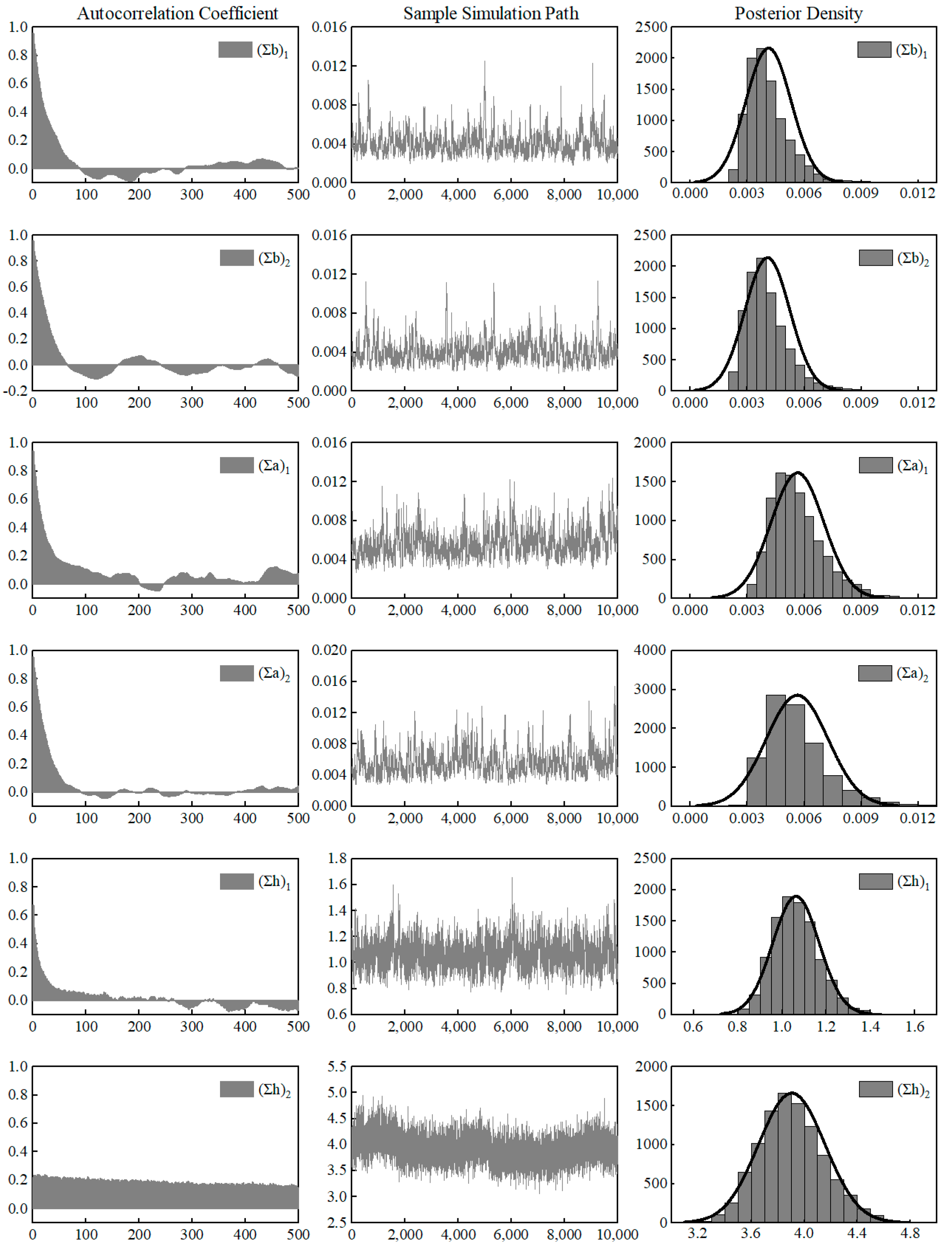
3.1. Parameter Estimation and Model Verification

Sampling results before convergence does not lead to stable distribution; therefore, when using the MCMC method to estimate the model parameters, burn on 10,000 times before sampling. The mean, standard deviation, 95% confidence interval, Geweke convergence diagnosis statistics, and the number of invalid factors of the posterior distribution of parameters were calculated. The results are shown in

Table 2. Parameter estimation results of TVP-SV-VAR model.

Parameter	Mean	Std	95% Interval	Geweke	Inefficiency
${\left({{\displaystyle \sum }}_{\beta }\right)}_1$	0.0041	0.0012	(0.0025, 0.0070)	0.384	41.65
${\left({{\displaystyle \sum }}_{\beta }\right)}_2$	0.0041	0.0012	(0.0024, 0.0071)	0.609	36.97
${\left({{\displaystyle \sum }}_a\right)}_1$	0.0056	0.0014	(0.0036, 0.0090)	0.000	61.45
${\left({{\displaystyle \sum }}_a\right)}_2$	0.0056	0.0016	(0.0034, 0.0098)	0.235	44.10
${\left({{\displaystyle \sum }}_h\right)}_1$	1.0629	0.1051	(0.8813, 1.2879)	0.600	29.34
${\left({{\displaystyle \sum }}_h\right)}_2$	3.9061	0.2497	(3.4574, 4.4399)	0.000	75.99

. It is shown that the Geweke statistics of the six estimation results are significantly lower than 1.96, and the original assumption that sampling results leads to a posteriori distribution cannot be rejected. The invalidity factor is less than 100, indicating that at least one irrelevant sample can be obtained in every 100 samples. The sampling effect is good enough to fit the posterior distribution.

In the process of solving the model using the MCMC method, the parameter autocorrelation diagram, sample simulation path diagram, and the fitted posterior distribution density function are shown in Figure 2. The autocorrelation diagram shows that the autocorrelation converges of $\left({{\displaystyle \sum }}_{\beta }\right)$, $\left({{\displaystyle \sum }}_a\right)$, and ${\left({{\displaystyle \sum }}_h\right)}_1$ rapidly reduce to 0. The convergence speed of ${\left({{\displaystyle \sum }}_a\right)}_1$ is slower than other parameters, which corresponds to the large invalid factor reflected in Table 2. The autocorrelation coefficient of ${\left({{\displaystyle \sum }}_h\right)}_2$ decreases slowly near 0.2. In the sample path map, its concentration is high, the extreme values appear less, and the sample path is stable. It can be found from the posterior distribution density function diagram of parameters that the sample results of six parameters $\left({{\displaystyle \sum }}_{\beta }\right)$, $\left({{\displaystyle \sum }}_a\right)$, and $\left({{\displaystyle \sum }}_h\right)$ are normally distributed, and the sample effect is good.

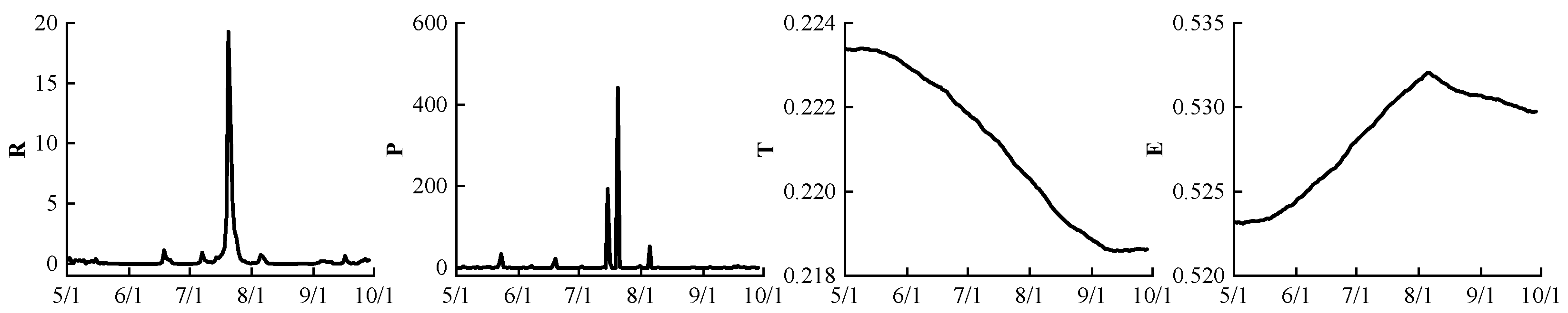
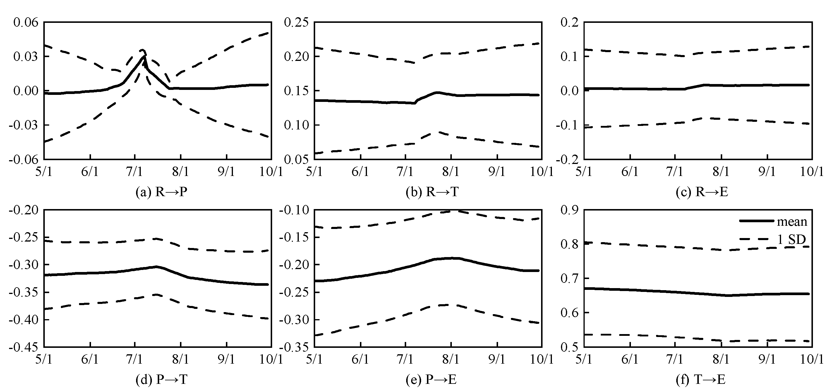
3.2. A Posteriori Estimation of Stochastic Volatility and Simultaneous Impulse Response Analysis

The posterior estimates of the stochastic volatility of runoff, precipitation, temperature, and evaporation were calculated, as shown in Figure 3. It can be seen that the variance of each variable fluctuated significantly over time, which further verified the rationality of the stochastic volatility of variance of the TVP-SV-VAR mode. The stochastic volatility of runoff and precipitation is the largest. There are two peaks of precipitation from 15 July to 21 July, while it remains low and relatively stable in other months. The stochastic volatility of runoff peaks on 21 July, which is in strong synchronization with precipitation. The stochastic volatility of temperature shows a downward trend near 0.2. The stochastic volatility of evaporation increases first and then decreases near 0.5, and there is an inflection point on 6 August after heavy rainfall. The traditional VAR model assumes the same variance, and the variance of the measured four variables fluctuates obviously with time. This is contrary to the assumption that the traditional VAR model has the same variance. Therefore, the TVP-SV-VAR model, which allows variable variance, is more suitable when analyzing the response of runoff to the variability of meteorological factors.

The impulse response results of different variables at all points were calculated by using the time-varying parameters of the model. Simultaneous impulse response analysis diagrams are drawn in Figure 4. The solid black line represents the posterior mean, and the dotted line represents the upper and lower bounds of the 95% confidence interval, respectively. In Figure 4a,c, the confidence interval of the simultaneous impulse response of runoff and precipitation, runoff and evaporation are included the x-axis. The response result is not significantly different from 0, indicating that the change of runoff will not have a simultaneous impact on precipitation and evaporation. In early July, the simultaneous response of runoff and precipitation fluctuate due to continuous heavy precipitation. It can be seen from Figure 4b,f that the runoff change has a positive impact on temperature of about 0.15, which decreases slightly with seasonal change. The temperature variability has a positive impact on evaporation at the spot of 0.7. Figure 4d,e shows that the variability of precipitation has a negative immediate impact on temperature and evaporation, that is, the increase in precipitation will lead to a decrease in temperature and evaporation in the same period. On the contrary, a decrease in evaporation and temperature will cause an increase in precipitation. In general, the immediate impulse response between temperature and evaporation is the largest. The simultaneous impact of precipitation and evaporation on runoff is close to 0 and other simultaneous impulse responses are between 0.1 and 0.3.

4. Discussion

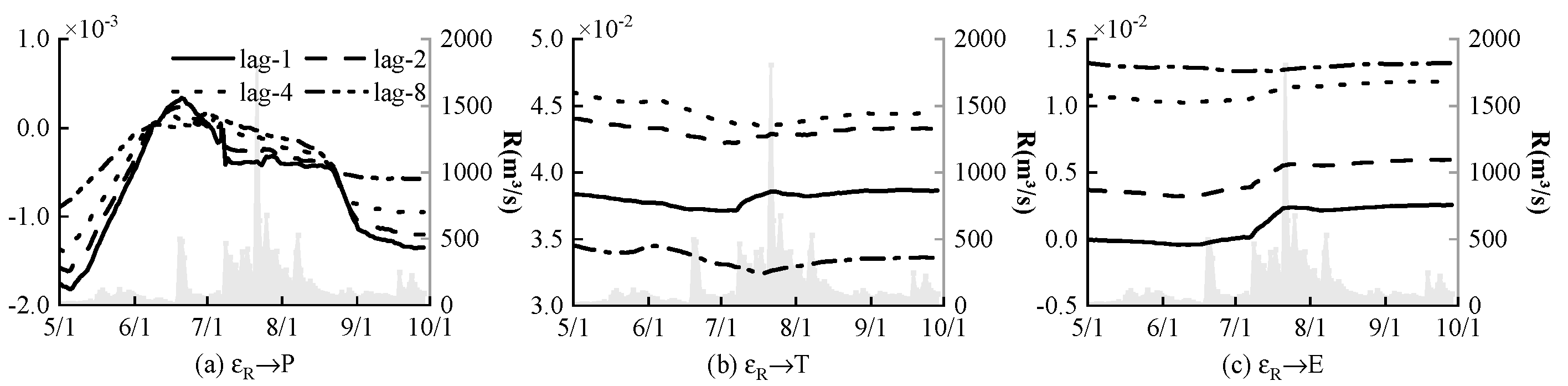
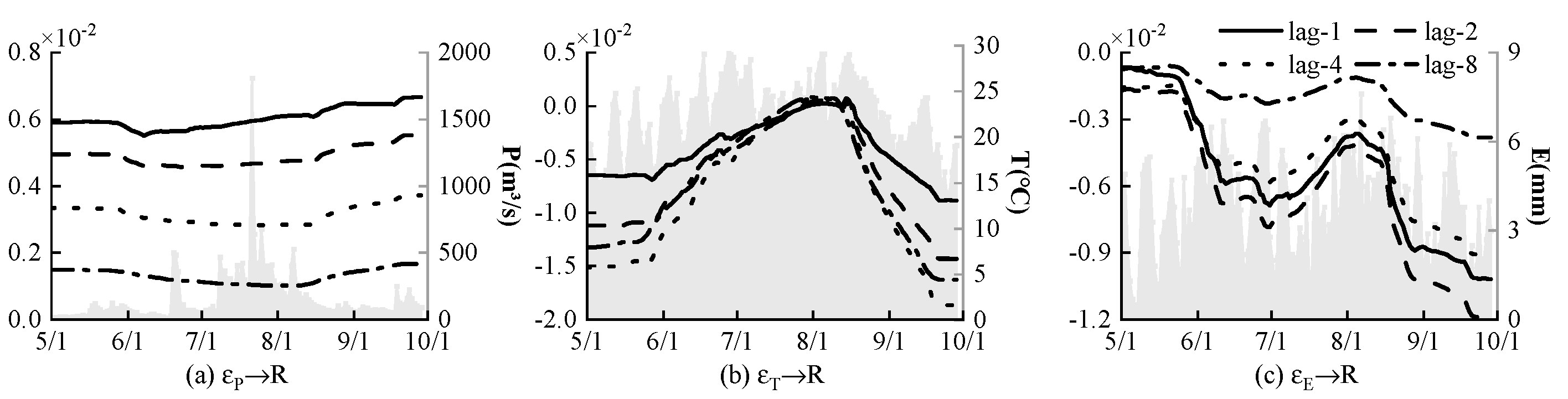
4.1. Pulse Response Analysis with Different Delays

The lag periods were selected as 1 day, 2 days, 4 days and 8 days. The impulse response diagrams of time-varying parameters were drawn, as shown in Figure 5, Figure 6, Figure 7 and Figure 8. The time-varying impulse response curves of different lag periods are very different. Figure 5 shows the impact of runoff change on precipitation, temperature, and evaporation in different lag periods. The negative pulse generated by runoff on precipitation gradually increases towards the middle of May and turns into a positive pulse, which decreases to 0 in early June and then continues to decrease. Runoff changes have negative pulse effects on most precipitation, and the response degree of precipitation decreases gradually with the increase in lag period. Runoff has a positive impact on temperature as a whole. By increasing the lag period, the impact first increases and then decreases, and reaches a greater value when the lag time is 4 days. Runoff change also has a positive impact on evaporation, but the impact gradually increases as lag time increases.

Figure 6 shows the impulse response of runoff to the variability of precipitation, temperature, and evaporation under different lag periods. Among them, runoff has a positive impulse response to precipitation variability, and the impulse response in different months fluctuates near a stable value. The lag of precipitation on runoff is not strong, and the response is most obvious when the lag time is 1 day. With an increase in lag time, the response becomes weaker. The runoff has a negative impulse response to temperature variability affected by the season, except in summer. There is almost no impulse response in early July and the influence of temperature on runoff is the most obvious when the lag time is 4 days. Runoff has a negative impulse response to evaporation variability, which fluctuates in July. Generally speaking, the negative impulse becomes larger with the passing of time. The response of runoff to evaporation variability is strongest when the lag time is 2 days, the second when the lag time is 1 day, and the weakest when the lag time is 8 days.

Figure 7 shows the mutual impulse response between precipitation, temperature, and evaporation under different lag periods. It can be seen that the impulse response of precipitation to temperature and evaporation variability varies greatly in different months, while the impact of precipitation variability on temperature and evaporation remains at the same level under the same lag period.

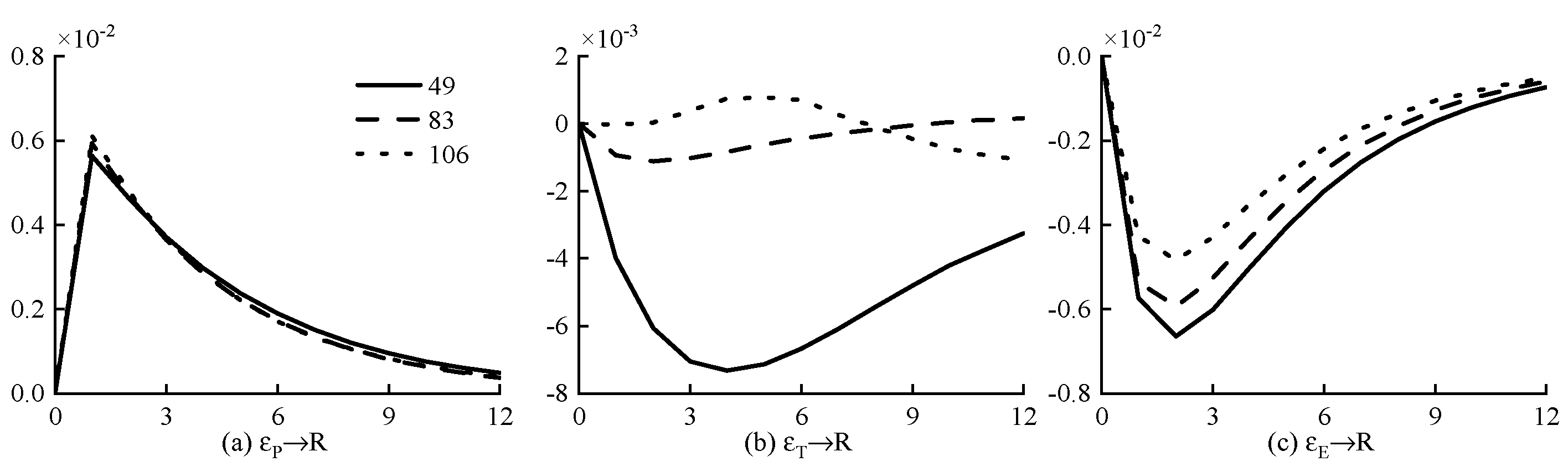
4.2. Pulse Response Analysis with Different Time Points

Three nodes of runoff were selected to analyze the response of runoff to the variability of precipitation, temperature, and evaporation, which are the minimum value (12 m³/s Node 49), mean value (150 m³/s Node 106), and maximum value (1810 m³/s Node 83), respectively. As shown in Figure 8, several conclusions can be reached. Firstly, runoff has a positive impulse response to precipitation, while it has a negative impulse response to temperature and evaporation. The increase in precipitation leads to an increase in runoff, while the increase in temperature and evaporation leads to a decrease in runoff. These are consistent with the actual hydrological characteristics, and the feasibility of the model is well demonstrated. Secondly, the response of different runoffs to precipitation and evaporation is similar, but the amount of runoff plays a decisive role in its response to temperature variability. When the runoff is small, the negative impact of temperature variability on runoff is large. When the runoff is large, the influence of temperature on runoff is not obvious. Finally, the influence of degree of precipitation, evaporation, and temperature on runoff increases first and then decreases with time. The impact of precipitation on runoff reaches the inflection point when t = 2, while the impact of evaporation on runoff reaches the inflection point when t = 3. Hence, the response of runoff to precipitation is more sensitive than that of evaporation. The sensitivity of runoff to temperature depends on runoff. To a certain extent, the impact of temperature on the runoff reaches the peak earlier when the runoff is large. The above model results are consistent with the actual hydrological characteristics of the Weihe River Basin.

4.3. Implications of TVP-SV-VAR Model

Simultaneous impulse response analysis is one element of the TVP-SV-VAR model which is different from the VAR model. The MCMC method is suitable to estimate the time-varying parameters of the model and to calculate the impulse response results of runoff to precipitation, temperature, and evaporation at all time points. In case of a severe rainstorm or sudden variability of temperature in a short time, the immediate response of runoff can be calculated through the model. It is of great significance for scientific response to extreme meteorological events, and for water resource management and regulation.

4.4. Limitations of TVP-SV-VAR Model

During research, we found that if the model sequence is too long, such as the simulation analysis of 30-year daily runoff data, the fitting effect will decline. In subsequent research, we can consider how to improve the fitting effect of the model in the simulation of long-time series. Moreover, we have only considered simple stochastic volatility processes. It would be useful to develop similar sampling methods for other richer stochastic volatility models, such as Eisenstat and Strachan [43]. All parameters were set to be time-varying, and then the parameters were estimated through MCMC sampling, but the benefits of the model may only come from the time-varying of a certain parameter. To investigate the individual contributions of time-varying coefficients, we can set some parameters to time variable and others to time invariant.

5. Conclusions

In this paper, time-varying parameters and stochastic volatility were applied with the vector autoregressive model. Then, a TVP-SV-VAR model of daily runoff response to the variability of meteorological factors was established by estimating the parameters using an MCMC. This model avoids the hypothesis of homoscedasticity of variance and allows the variance to be randomly variable, which is more practical and reasonable. Taking the Linjiacun hydrological station as a case study, the main conclusions are as follows:

(1)

The posterior estimates of the stochastic volatility of runoff, precipitation, temperature, and evaporation vary significantly with time, and the variance fluctuations of runoff and precipitation have strong synchronicity.

(2)

The impact of precipitation and evaporation on the simultaneous pulse of runoff is close to 0. The simultaneous impulse response between temperature and evaporation is the largest.

(3)

Runoff has a positive impulse response to precipitation, which decreases with the increase in lag time. It has a negative impulse response to temperature and evaporation, which fluctuates greatly. The response speed is precipitation > evaporation > temperature.

(4)

When the runoff has different statistical values, the response curves to precipitation and evaporation are similar, and the response to temperature variability is more complex.

The TVP-SV-VAR model can analyze the dynamic impulse response of runoff to meteorological factors, including different lag times and different time nodes, to provide a reliable basis for the attribution analysis of runoff change.

References

1. Huntington, T.G. Evidence for intensification of the global water cycle: Review and synthesis. J. Hydrol. 2006, 319, 83–95. [Google Scholar] [CrossRef]
2. Pendergrass, A.G.; Knutti, R.; Lehner, F.; Deser, C.; Sanderson, B.M. Precipitation variability increases in a warmer climate. Sci. Rep. 2017, 7, 17966. [Google Scholar] [CrossRef] [Green Version]
3. Jia, Q.; Li, M.; Dou, X. Climate Change Affects Crop Production Potential in Semi-Arid Regions: A Case Study in Dingxi, Northwest China, in Recent 30 Years. Sustainability 2022, 14, 3578. [Google Scholar] [CrossRef]
4. Rahimi, J.; Malekian, A.; Khalili, A. Climate change impacts in Iran: Assessing our current knowledge. Theor. Appl. Climatol. 2019, 135, 545–564. [Google Scholar] [CrossRef]
5. Azad, A.S.; Sokkalingam, R.; Daud, H.; Adhikary, S.K.; Khurshid, H.; Mazlan, S.N.; Rabbani, M.B. Water Level Prediction through Hybrid SARIMA and ANN Models Based on Time Series Analysis: Red Hills Reservoir Case Study. Sustainability 2022, 14, 1843. [Google Scholar] [CrossRef]
6. Zhu, T.; Lund, J.R.; Jenkins, M.W.; Marques, G.F.; Ritzema, R.S. Climate change, urbanization, and optimal long-term floodplain protection. Water Resour. Res. 2007, 43, W06421. [Google Scholar] [CrossRef] [Green Version]
7. Bermúdez, M.; Farfán, J.F.; Willems, P.; Cea, L. Assessing the Effects of Climate Change on Compound Flooding in Coastal River Areas. Water Resour. Res. 2021, 57, e2020WR029321. [Google Scholar] [CrossRef]
8. Jamali, B.; Bach, P.M.; Deletic, A. Rainwater harvesting for urban flood management—An integrated modelling framework. Water Res. 2020, 171, 115372. [Google Scholar] [CrossRef] [PubMed]
9. Marques, A.C.; Veras, C.E.; Rodriguez, D.A. Assessment of water policies contributions for sustainable water resources management under climate change scenarios. J. Hydrol. 2022, 608, 127690. [Google Scholar] [CrossRef]
10. Peña-Angulo, D.; Vicente-Serrano, S.M.; Domínguez-Castro, F.; Lorenzo-Lacruz, J.; Murphy, C.; Hannaford, J.; Allan, R.P.; Tramblay, Y.; Reig-Gracia, F.; El Kenawy, A. The Complex and Spatially Diverse Patterns of Hydrological Droughts across Europe. Water Resour. Res. 2022, 58, e2022WR031976. [Google Scholar] [CrossRef]
11. Zhou, Z.; Shi, H.; Fu, Q.; Ding, Y.; Li, T.; Liu, S. Investigating the Propagation From Meteorological to Hydrological Drought by Introducing the Nonlinear Dependence With Directed Information Transfer Index. Water Resour. Res. 2021, 57, e2021WR030028. [Google Scholar] [CrossRef]
12. Deb, P.; Kiem, A.S.; Willgoose, G. Mechanisms influencing non-stationarity in rainfall-runoff relationships in southeast Australia. J. Hydrol. 2019, 571, 749–764. [Google Scholar] [CrossRef]
13. Zhou, Z.; Ding, Y.; Shi, H.; Cai, H.; Fu, Q.; Liu, S.; Li, T. Analysis and prediction of vegetation dynamic changes in China: Past, present and future. Ecol. Indic. 2020, 117, 106642. [Google Scholar] [CrossRef]
14. Narsimlu, B.; Gosain, A.K.; Chahar, B.R. Assessment of Future Climate Change Impacts on Water Resources of Upper Sind River Basin, India Using SWAT Model. Water Resour. Manag. 2013, 27, 3647–3662. [Google Scholar] [CrossRef]
15. Tan, X.; Liu, B.; Tan, X. Global Changes in Baseflow Under the Impacts of Changing Climate and Vegetation. Water Resour. Res. 2020, 56, e2020WR027349. [Google Scholar] [CrossRef]
16. Balaganesh, G.; Malhotra, R.; Sendhil, R.; Sirohi, S.; Maiti, S.; Ponnusamy, K.; Sharma, A.K. Development of composite vulnerability index and district level mapping of climate change induced drought in Tamil Nadu, India. Ecol. Indic. 2020, 113, 106197. [Google Scholar] [CrossRef]
17. Kilinc, H.C.; Yurtsever, A. Short-Term Streamflow Forecasting Using Hybrid Deep Learning Model Based on Grey Wolf Algorithm for Hydrological Time Series. Sustainability 2022, 14, 3352. [Google Scholar] [CrossRef]
18. Jin, H.; Rui, X.; Li, X. Analysing the Performance of Four Hydrological Models in a Chinese Arid and Semi-Arid Catchment. Sustainability 2022, 14, 3677. [Google Scholar] [CrossRef]
19. Wang, H.; Wang, W.; Du, Y.; Xu, D. Examining the Applicability of Wavelet Packet Decomposition on Different Forecasting Models in Annual Rainfall Prediction. Water 2021, 13, 1997. [Google Scholar] [CrossRef]
20. Thapa, S.; Li, H.; Li, B.; Fu, D.; Shi, X.; Yabo, S.; Lu, L.; Qi, H.; Zhang, W. Impact of climate change on snowmelt runoff in a Himalayan basin, Nepal. Environ. Monit. Assess. 2021, 193, 393. [Google Scholar] [CrossRef]
21. Song, Y.; Zhang, J.; Zhang, M. Impacts of Climate Change on Runoff in Qujiang River Basin Based on SWAT Model. In Proceedings of the 2018 7th International Conference on Agro-Geoinformatics (Agro-Geoinformatics), Hangzhou, China, 6–9 August 2018; pp. 1–5. [Google Scholar]
22. Ya-qin, Q. Impact of climate change on runoff process in headwater area of the Yellow River. J. Hydraul. Eng. 2008, 39, 52–58. [Google Scholar]
23. Zakizadeh, H.R.; Ahmadi, H.; Zehtabiyan, G.R.; Moeini, A.; Moghaddamnia, A. Impact of climate change on surface runoff: A case study of the Darabad River, northeast of Iran. J. Water Clim. Chang. 2020, 12, 82–100. [Google Scholar] [CrossRef]
24. Wang, H.; Chen, F. Increased stream flow in the Nu River (Salween) Basin of China, due to climatic warming and increased precipitation. Geogr. Ann. Ser. A Phys. Geogr. 2017, 99, 327–337. [Google Scholar] [CrossRef]
25. Yuan, X.; Jiao, Y.; Yang, D.; Lei, H. Reconciling the Attribution of Changes in Streamflow Extremes From a Hydroclimate Perspective. Water Resour. Res. 2018, 54, 3886–3895. [Google Scholar] [CrossRef]
26. Ji, P.; Yuan, X.; Ma, F.; Pan, M. Accelerated hydrological cycle over the Sanjiangyuan region induces more streamflow extremes at different global warming levels. Hydrol. Earth Syst. Sci. 2020, 24, 5439–5451. [Google Scholar] [CrossRef]
27. Radchenko, I.; Dernedde, Y.; Mannig, B.; Frede, H.-G.; Breuer, L. Climate change impacts on runoff in the Ferghana Valley (Central Asia). Water Resour. 2017, 44, 707–730. [Google Scholar] [CrossRef]
28. Lopez, S.R.; Hogue, T.S.; Stein, E.D. A framework for evaluating regional hydrologic sensitivity to climate change using archetypal watershed modeling. Hydrol. Earth Syst. Sci. 2012, 17, 3077–3094. [Google Scholar] [CrossRef]
29. Jones, R.N.; Chiew, F.H.S.; Boughton, W.C.; Zhang, L. Estimating the sensitivity of mean annual runoff to climate change using selected hydrological models. Adv. Water Resour. 2006, 29, 1419–1429. [Google Scholar] [CrossRef] [Green Version]
30. Legesse, D.; Abiye, T.A.; Vallet-Coulomb, C.; Abate, H. Streamflow sensitivity to climate and land cover changes: Meki River, Ethiopia. Hydrol. Earth Syst. Sci. 2010, 14, 2277–2287. [Google Scholar] [CrossRef] [Green Version]
31. Raghavan, R.; Rao, K.V.; Shirahatti, M.S.; Srinivas, D.K.; Reddy, K.S.; Chary, G.R.; Gopinath, K.A.; Osman, M.; Prabhakar, M.; Singh, V.K. Assessment of Spatial and Temporal Variations in Runoff Potential under Changing Climatic Scenarios in Northern Part of Karnataka in India Using Geospatial Techniques. Sustainability 2022, 14, 3969. [Google Scholar] [CrossRef]
32. Li, Y.; Mao, J.; Zhang, M.; Yue, C. Relationship between meteorological elements and runoff in Jingou River Basin of Xinjiang based on the VAR model. J. Water Resour. Water Eng. 2020, 31, 80–86. [Google Scholar]
33. Primiceri, G.E. Time Varying Structural Vector Autoregressions and Monetary Policy. Rev. Econ. Stud. 2005, 72, 821–852. [Google Scholar] [CrossRef]
34. Chan, J.C.C.; Eisenstat, E. Bayesian model comparison for time-varying parameter VARs with stochastic volatility. J. Appl. Econom. 2018, 33, 509–532. [Google Scholar] [CrossRef]
35. Nakajima, J. Time-Varying Parameter VAR Model with Stochastic Volatility: An Overview of Methodology and Empirical Applications. Monet. Econ. Stud. 2011, 29, 107–142. [Google Scholar]
36. Kastner, G. Sparse Bayesian time-varying covariance estimation in many dimensions. J. Econom. 2019, 210, 98–115. [Google Scholar] [CrossRef]
37. Jebabli, I.; Arouri, M.; Teulon, F. On the effects of world stock market and oil price shocks on food prices: An empirical investigation based on TVP-VAR models with stochastic volatility. Energy Econ. 2014, 45, 66–98. [Google Scholar] [CrossRef]
38. McCauley, R.N.; McGuire, P.; Sushko, V. Global dollar credit: Links to US monetary policy and leverage. Econ. Policy 2015, 30, 187–229. [Google Scholar] [CrossRef]
39. Heshmatol Vaezin, S.M.; Moftakhar Juybari, M.; Sadeghi, S.M.; Banaś, J.; Marcu, M.V. The Seasonal Fluctuation of Timber Prices in Hyrcanian Temperate Forests, Northern Iran. Forests 2022, 13, 761. [Google Scholar] [CrossRef]
40. Krämer, W. Fractional integration and the augmented Dickey–Fuller Test. Econ. Lett. 1998, 61, 269–272. [Google Scholar] [CrossRef] [Green Version]
41. Wang, P.; Tang, Y.; Joo Bae, S.; He, Y. Bayesian analysis of two-phase degradation data based on change-point Wiener process. Reliab. Eng. Syst. Saf. 2018, 170, 244–256. [Google Scholar] [CrossRef]
42. Luo, C.; Shen, L.; Xu, A. Modelling and estimation of system reliability under dynamic operating environments and lifetime ordering constraints. Reliab. Eng. Syst. Saf. 2022, 218, 108136. [Google Scholar] [CrossRef]
43. Eisenstat, E.; Strachan, R.W. Modelling Inflation Volatility. J. Appl. Econom. 2016, 31, 805–820. [Google Scholar] [CrossRef] [Green Version]
Figure 1. Runoff, precipitation, temperature, and evaporation data of a control basin above Linjiacun from 1 May to 30 September 2013.
Sustainability 14 06989 g001
Figure 2. Results of simulation of TVP-SV-VAR model parameters by MCMC method.
Sustainability 14 06989 g002
Figure 3. Posterior estimates of stochastic fluctuations in runoff, precipitation, temperature, and evaporation.
Sustainability 14 06989 g003
Figure 4. Analysis curve of simultaneous pulse response.
Sustainability 14 06989 g004
Figure 5. Effects of runoff variation on precipitation, temperature, and evaporation under different lag periods.
Sustainability 14 06989 g005
Figure 6. Impulse response of runoff to precipitation, temperature, and evaporation under different lag periods.
Sustainability 14 06989 g006
Figure 7. Impulse response among precipitation, temperature, and evaporation under different lag periods.
Sustainability 14 06989 g007
Figure 8. Pulse response of runoff to precipitation, temperature, and evaporation at different time nodes.
Sustainability 14 06989 g008