Abstract
Pavement performance prediction is necessary for road maintenance and repair (M&R) management and plans. The accuracy of performance prediction affects the allocation of maintenance funds. The international roughness index (IRI) is essential for evaluating pavement performance. In this study, using the road pavement data of LTPP (Long-Term Pavement Performance), we screened the feature parameters used for IRI prediction using the mean decrease impurity (MDI) based on random forest (RF). The effectiveness of this feature selection method was proven suitable. The prediction accuracies of four promising prediction models were compared, including Gradient Boosting Decision Tree (GBDT), eXtreme Gradient Boosting (XGBoost), support vector machine (SVM), and multiple linear regression (MLR). The two integrated learning algorithms, GBDT and XGBoost, performed well in prediction. GBDT performs best with the lowest root mean square error (RMSE) of 0.096 and the lowest mean absolute error (MAE) of 6.2% and the coefficient of determination (R2) reaching 0.974. However, the prediction accuracy varies in numerical intervals, with some deviations. The stacking fusion model with a powerful generalization capability is proposed to build a new prediction model using GBDT and XGBoost as the base learners and bagging as the meta-learners. The R2, RMSE, and MAE of the stacking fusion model are 0.996, 0.040, and 1.3%, which further improves the prediction accuracy and verifies the superiority of this fusion model in pavement performance prediction. Besides, the prediction accuracy is generally consistent across different numerical intervals.
1. Introduction
Pavement performance prediction is a prerequisite for maintenance and repair (M&R) planning. Its prediction accuracy has a non-negligible impact on allocating funds [1,2,3,4]. In the whole life cycle of M&R planning, accurate predictions of pavement performance indicators are required to optimize funds and define the M&R projects. M&R timing is usually determined based on predictions, and a delayed or early M&R action may result in wasted money, energy consumption, and traffic disruptions. However, the survey task may not cover all road sections. For the road sections that are not covered, prediction can help manage agents to keep track of the pavement condition in time to prevent losses due to untimely awareness of indicators exceeding the specified thresholds.
The international roughness index (IRI) is an essential indicator calculated based on the longitudinal profile of the wheel track. The pavement condition index (PCI) is a statistical indicator based on the pavement distresses. Due to the heavy survey work, scholars and road management agencies have tried to establish correlations of different evaluation indicators. A sigmoid function is found to best express the relationship between PCI and IRI with a coefficient of determination (R2) of 0.995; the model validation using a different dataset also yielded highly accurate predictions (R2 = 0.99) [5]. Although the prognosis of PCI by IRI reduces the detection and analysis work, it ignores the more critical pavement distress information, which has been mentioned by Kırbas [6]. This neglect may lead to a significant bias when applying this prognosis to the forecasting domain.
Time-series-based model prediction methods often group data based on external factors such as time, environment, and traffic and carry out performance prediction with road age as the independent variable. Abaza found that the transfer probability estimated by the Markov-based pavement performance prediction model became very unstable as the section length became more prominent and the sample size became smaller [7]. The global prediction precision values for the five performance indicators (PIs), namely cracking, skid resistance, bearing capacity, longitudinal roughness, and transverse roughness, by a practical application of a Markov model are 77, 71, 94, 83, and 80%, respectively [8]. Mohammadi et al. [9] pointed out that environmental conditions have overshadowed traffic loading by faster PCI and IRI degradation for local segments with less traffic load than arterial ones based on a review of deterministic models.
Analyzing critical features affecting performance indices can aid design and M&R management. No.-200-passing, hydraulic conductivity, and equivalent single-axle loads in thousands (KESAL) are essential factors predicting IRI [3]. A sensitivity analysis showed that the machine learning models are susceptible to previous IRI values, and variations in the remaining variables showed little effect on the machine learning models [10]. Ali et al. [11] found that almost all the distresses, including rutting, block cracking, fatigue, transverse cracking, and potholes, negatively affected the IRI value except delamination, patching, and longitudinal cracking by an IRI pavement distress model with the p-value of 0.05. Onayer and Swei [12] emphasized to the reader the fact that parameter estimates are sensitive to the selected time range of consecutive IRI measurements. There is some conflict in the findings of these studies. Correlation analysis may not accurately reflect the contribution of the distress to IRI.
Accurate predictions of performance indicators can be used for M&R planning and compensate for inadequate survey data coverage. Attempts have been made to use machine learning and deep learning algorithms to improve the accuracy of predicting the IRI. The Random Forest Regression (RFR) addressed the overfitting issue significantly better than the linear regression model [13]. Marcelino et al. [14] also found that the RFR achieved excellent predictive performance in training and testing sets. Based on conducting a meta-analysis based on inverse variance heterogeneity for 20 studies conducted between 2001 and 2020, RF was found to be the most accurate technique, with an overall performance value of 0.995; however, the machine learning algorithm captured an average of 15.6% more variability than traditional techniques [15]. Gene expression programming (GEP) achieved the highest accuracy in predicting the remaining service life compared with support vector regression (SVR) and support vector regression optimized by the fruit fly optimization algorithm (SVR-FOA) [16]. Li et al. [1] found that the optimized support vector machine (SVM) has better rutting prediction performance and perfect generalization, which was higher than those of the unoptimized support vector machine model, and the model using particle swarm optimization has a fast convergence speed. Abdelaziz et al. [17] predicted IRI based on 506 road sections with 2439 observations, and the R2 value of the ANN (Artificial Neural Network) model was 0.75. Riding index, cracking index, and rutting index for the three pavement types ACC, PCC, and COM were predicted, and compared to the multiple linear regression (MLR) model, the ANN model based on weather factors (i.e., temperature, precipitation, and freeze-thaw cycles), traffic load, pavement age, SN, layer thickness, and subgrade stiffness for the Iowa highway, future pavement conditions are more accurately predicted [18]. Hossain et al. [19] demonstrated that the ANN-based IRI prediction model is reasonable for short-term and long-term pavement observation IRI data, and the root mean square error (RMSE) value of the test results was as low as 0.027. A more accurate prediction was fine-tuned by a coupled use of RFR and ANN [20]. Choi and Myungsik Do [2] predicted the deterioration of pavement performance with a recurrent neural network algorithm with a high coefficient of determination of 0.71–0.87 by using monitoring data from the Korean National Highway Pavement Management System. Marcelino et al. [14] used a transfer learning approach based on a boosting algorithm to develop pavement performance regression models with limited data contexts achieving a prediction accuracy improvement of approximately 6%. Basher et al. [15] pointed out that ANN was considered an effective technique based on its accurate predictions of small and large samples. The gradient boosting machine (GBM) models were better than other machine learning methods [21,22].
Some typical IRI prediction models and their accuracies are summarized, as shown in Table 1.

Table 1.
Summary of Predictive Models.
As shown in Table 1, the inclusion of other pavement performance feature parameters can improve R2 and reduce the error. However, the role of rich and detailed parameters of structural and environmental features still cannot be ignored. The overall performances of ANN and RF are similar. When the dataset is the same one, RF usually performs better than ANN, XGBoost [3], GBM [22], and LightGBM [21], and all perform better than RF. In addition, the performance of SVM and MLR models based on the same dataset has achieved about 50% lower R2 values than ANN.
RF, SVM, MLR, and ANN are widely used for pavement performance prediction. Boosting algorithms can significantly improve the prediction accuracy of machine learning models with lower RMSE and MAE. Hence, we chose two boosting algorithms, MLR and SVM, to make the prediction.
Project-level M&R planning is often done in segments. Since the segments have the same environmental conditions, similar traffic conditions, and almost the same structure and material types, feature-based prediction methods are not supported by sufficient data, and time-series-based predictions suffer from low accuracy. Given that a 10% deviation from the forecast results in a 16% increase in costs and a 2% decrease in benefits over the whole life cycle (20 years) [19], project-level application requirements for MAE should not exceed 10%. Therefore, we need a machine learning prediction model that does not depend on net-level features and time-series data, so its main features should be survey data of the base year. The detailed distress, pavement age, and traffic data were chosen for contribution rates analysis to select feature parameters. To enhance MAE, we constructed a stacking fusion model based on two relatively good prediction models to see if they still can be improved.
2. Data Preparation
The raw data are from the LTPP data across 62 cities, including: traffic volume size (76,989 data), crack length (12,964 data), traffic opening date (1817 data), rut depth (18,128 data), IRI size (97,535 data), and texture information (18,735 data) in six tables, totaling 226,128 data. After removing the abnormal data, such as null values, we obtained 74,773 data with 41 feature parameters (Table 2). Although these features are correlated, excluding the directly calculated correlation indicators, this study does not perform any prior knowledge-based processing.
Table 2.
Description of the feature variables.
3. Methodology
3.1. Feature Selection Based on RF Algorithm
Feature selection serves the machine learning model, and good feature metric parameters help to improve the model fitting accuracy. Therefore, to ensure the accuracy of the pavement prediction model, the features with high relevance need to be selected as the training set for training the model. The two popular feature selection methods are the Pearson coefficient and Spearman coefficient methods. Pearson’s correlation, also known as product-difference correlation, is a method the British statistician Pearson proposed in the 20th century to calculate the linear correlation. It is one of the most commonly used correlation coefficients. It is denoted as and reflects the degree of linear correlation between two variables, X and Y. Suppose there are two variables, X and Y. The Pearson correlation coefficient between the two variables can be calculated by Equation (1).
where is the covariance between and , is the standard deviation of , and is the standard deviation of .
The Spearman coefficient () is a non-parametric measure of the relationship between two variables, which can be calculated by Equation (2).
where denotes the number of data, and denotes the difference between the two variables.
A shortcoming is that they are highly dependent on linear relationships, but complex linearity and nonlinearity exist between actual pavement survey data and predictive indicator data.
Usually, the importance of features can be reflected by the segmentation of node data based on RF. However, the double-random method in selecting training samples and node classification features may cause features with high discrimination to be chosen as segmentation attributes infrequently and features with low bias to be chosen as segmentation attributes more frequently. Therefore, simply using the frequency of features used as segmentation attributes to measure the importance does not accurately reflect the contribution of different features.
Breiman [25] proposed the mean decrease impurity (MDI) to identify the variable importance for predicting based on Random Forest by adding weighted impurity decreases for all nodes where the feature is used, averaged over all the trees in the forest. The RF-based variable selection determines a smaller number of relevant predictors and allows the construction of a more parsimonious model but with predictive performance [26].
The MDIs are calculated by Equation (3).
where , , and are the impurity value, the impurity value in the right child, and the impurity value in the left child, respectively. is the number of samples at the current node, is the number of samples in the right child, is the number of samples in the left child, and N is the sample size.
3.2. Accuracy Evaluation of MLR, GBDT, XGBoost, and SVM Models
We chose MLR, GBDT, XGBoost, and SVM models for a comparative study, which are all commonly used for pavement performance prediction.
GBDT is a machine learning algorithm proposed by Friedman [27] and is widely used in classification, regression, and recommendation systems for ranking tasks. The core idea of GBDT is to reduce the residuals, and each iteration of GBDT is to minimize the residuals generated by the previous iteration.
XGBoost [28] is an iterative, tree-like algorithm that combines multiple weak classifiers into one robust classifier, implementing a gradient-boosted decision tree (GBDT). XGBoost is a powerful sequential integration technique with a modular structure for parallel learning to achieve fast computation, preventing overfitting by regularization and generating weighted quantile sketches for processing weighted data. In the case of nonlinear regression tasks, kernel functions are used in SVM operations. By using nonlinear vector kernel functions, the original data can be mapped to a high-dimensional feature space, converting the nonlinear regression problem into a linear problem to be solved.
The IRI prediction models constructed based on the above four algorithms, namely GBDT, XGBoost, SVM, and MLR, were implemented on the Python 3.9.2 platform in the environment of Jupyter. The dataset is 74,773 data after data preprocessing in the previous paper, containing 41 features and 1 prediction value. The training and testing sets were divided in a 7:3 manner, and RMSE, MAE, and R2 were used to evaluate the machine learning models’ performance
RMSE and MAE are used to measure the closeness of the predicted value to the actual value, and a smaller value indicates a higher prediction accuracy; R2 is the expressiveness of the expected value to the actual value, and the larger R2 means the higher prediction accuracy (not more than 1). The three evaluation indicators were calculated according to Equations (4)–(6).
where is the number of the sample set ; is the measured value of IRI; is the predicted value of IRI, and is the mean of the measured value of IRI.
3.3. The Stacking Fusion Method
The stacking model fusion method first divides the original feature dataset into several sub-datasets, fed into each base learner of the layer one prediction model. Each base learner outputs its prediction results. The stacking model fusion method can improve the overall prediction accuracy by generalizing the output results of multiple models.
The original dataset is sliced and divided into the training and test sets according to a specific ratio in the first stage. Suitable base learners are selected to train the training set by cross-validation. After completing the training, each base learner is predicted on the validation and test sets. We should first figure out the machine learning models with relatively good prediction performance, ensuring the diversity between models. In the second stage, the prediction results of the base learners are used as the feature data for training and prediction of the meta-learner, respectively. The meta-learner combines the features obtained in the previous stage and the labels of the original training set for the sample data to build the model and output the final stacking model prediction results.
Two sets of predictions are obtained using two different integrated model algorithms with high prediction accuracy as base learners, and then, the three sets of predictions are applied to the second layer using a meta-learner, which is chosen to train the bagging model to obtain the final prediction results.
4. Results and Discussion
4.1. Feature Selection Results
The input port is used to receive the dataset passed down from the predecessor node, and the output port is used to output the dataset with the added discrete fields, where the top 20 results are shown in Figure 1.
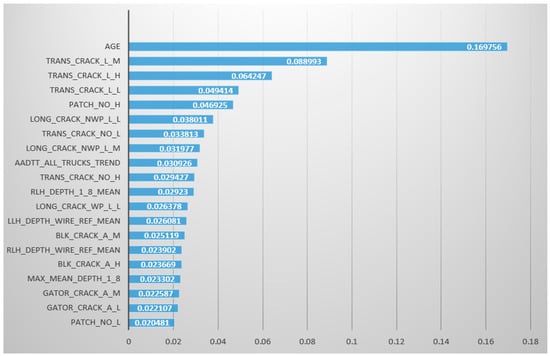
Figure 1.
Correlation analysis of feature parameters and IRI based on RF algorithm.
We can see from Figure 1 that road age (AGE) is the most crucial factor affecting pavement levelness, which is consistent with the concept of prediction based on deterministic models and time series and is also compatible with the findings of correlation analysis. Except for traffic volume, the rest of the characteristic critical indicators belong to pavement distresses. AADTT and AGE are all related to cumulative loads, and the road age also includes the cumulative effect from the environment.
Among the various types of distresses, the effect of transverse cracks is at the top. At the same time, the impact of rut depth, which also represents the roughness characteristics of the pavement, was not significant. The results imply that the correlation model that only considers the macroscopic damage state of the pavement without considering the specific damage types is not scientific. The roughness is not only related to the pavement’s surface state but is also related to the overall structural condition of the road, which is the result of the combined effect of the environment and traffic load. This is why the age of the road has a more significant impact.
The feature data selected in this study, excluding road age, are easily achieved survey data that do not require establishing an extensive road asset database and provide greater convenience for road management work.
4.2. Accuracy Evaluation Results of MLR, GBDT, XGBoost, and SVM Models
Scatter plots of the comparison between predicted and actual values of the four prediction models are in Figure 2, Figure 3, Figure 4 and Figure 5. The lines represent the exact agreement between the predicted and actual values, and the data points above the lines represent predicted values that are large relative to the actual values. In contrast, the data points below the lines represent lower predicted values than the actual ones. It is not difficult to find that GBDT and XGBoost have significantly fewer outliers away from the regression line than SVM and multiple linear regression, which indicates that the prediction effects of GBDT and XGBoost are much better than the latter two. At the same time, SVM and XGBoost are not far from reaching the fit, so the prediction effects of these two algorithms are more general under this data set.
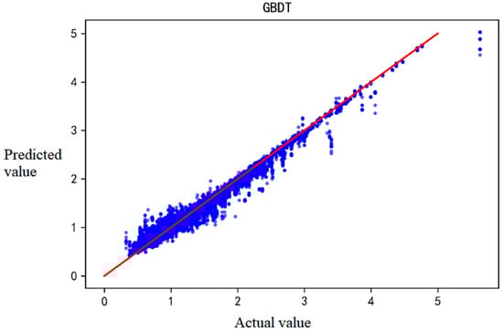
Figure 2.
The predicted IRI values and actual IRI values of GBDT-based prediction results.
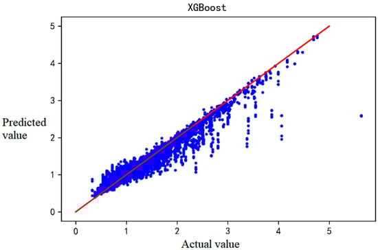
Figure 3.
The predicted and actual IRI values of XGBoost-based prediction results.
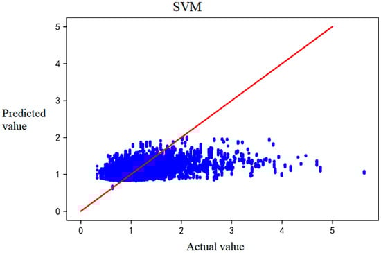
Figure 4.
The predicted and actual IRI values of SVM-based prediction results.
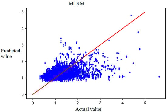
Figure 5.
The predicted and actual IRI values of MLRM-based prediction results.
Figure 2 shows that the GBDT model performs well and has achieved a good fit. However, when IRI is above 2, the predicted value seems lower. Figure 3 implies that XGBoost shows a similar trend with more deviations. As seen in Figure 4, the SVM model may have an insufficient fitting ability when the sample distribution is not uniform, especially in the interval with a small sample size. The deviation of MLR tends to increase with increasing IRI, but the positive and negative deviations are more uniform (Figure 5).
The values of RMSE, MAE, and R2 for the different prediction models are in Table 3. SVM and MLR perform even worse than the known datasets in the literature (Table 1), probably because the initial IRI data did not incorporate parameters. However, the prediction accuracy of GBDT and XGBOOST is significantly higher.
Table 3.
Evaluation results of MLR, GBDT, XGBoost, and SVM models.
From the prediction results of the four prediction models, the models can be divided into two groups: one group is GBDT and XGBoost, representing integrated learning, and the other group is SVM and MLR, representing weak learners. SVM and MLR can better characterize the mapping relationship under small samples than GBDT and XGBoost. Still, they are weak learners, while GBDT and XGBoost belong to integrated algorithms assembled by a series of weak learners (decision trees). While GBDT and XGBoost are the weight-boosting algorithms, the prediction accuracy is inevitably stronger than that of a single weak learner in the case of complex pavement data structure because of the correction feature of the boosting algorithm.
The values of R2 for GBDT and XGBoost are 0.974 and 0.925, and the R2 values of SVM and MLR are almost 70% lower. We can indicate that the predicted values of GBDT and XGBoost are closer to the actual values in the prediction process of the IRI of pavement. Both the accuracies of GBDT and XGBoost can meet the requirements of net-level forecasting. However, MAE values (6.2% and 8.4%) for GBDT and XGBoost are close to 10%, and data on specific value intervals have relatively high absolute errors.
4.3. Evaluation of the Stacking Fusion Model
We then fused the two algorithms in a stacking way to improve their prediction accuracies in different threshold ranges. To verify the superiority of the stacking fusion model in IRI prediction, the training and test sets with the previous four prediction models were maintained and compared. The values of the three evaluation indicators (MSE, MAE, and R2) for the stacking fusion model are in Table 3. It is found that the stacking fusion model yields an improvement in each evaluation indicator.
The RMSE value of the stacking fusion model is 58% lower than GBDT and 75% lower than XGBoost; its MAE is 79% lower than GBDT and 85% lower than XGBoost, while R2 is 2% higher than GBDT and 8% higher than XGBoost. The accuracy of the stacking fusion model is further improved compared with the GBDT and XGBoost models.
Figure 6 shows the scatter plot of the actual and predicted IRI values of the stacking fusion model, the meanings of points and lines are the same as Figure 2, Figure 3, Figure 4 and Figure 5. The stacking fusion model, based on the original GBDT and XGBoost, further approximates the regression line in the scatter plot, indicating that the overall predicted values of the fusion model are closer to the actual values in the prediction process. The fusion model obtained more minor errors and performed better, especially for larger values of IRI, and may be usable for project-level forecasting.
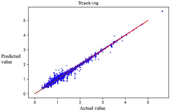
Figure 6.
Stacking fusion-based prediction results.
5. Conclusions
Based on LTPP data across 62 cities, this study seeks prediction methods with better generalization ability and higher accuracy with the research objective of predicting the IRI of pavements. Traditional feature parameters such as structural and environment indicators that can only be obtained based on file collection or database building and used for network-level pavement performance prediction are discarded. We mainly focus on those survey data that can be observed easily.
(1) By selecting feature parameters based on the random forest prediction model, 20 indicators with certain influences that can be used to build the prediction model were identified. The accuracies of the prediction results imply the feather selection method is suitable.
(2) Excluding road age, the feature parameters selected in this study are all easily achieved detection data. It can be concluded that accuracy prediction does not require establishing an extensive road asset database and provides greater convenience for the management work.
(3) GBDT and XGBoost have achieved high R2 (0.974 and 0.925), which can meet the requirements of net-level forecasting. However, MAE values (6.2% and 8.4%) are close to 10%, and data on some specific value intervals have relatively high absolute errors.
(4) The accuracy of the stacking fusion model is further improved based on the original GBDT and XGBoost; the R2 is as high as 0.996, and the RMSE and MAE are only 0.04 and 13%.
(5) This study confirms the effectiveness of MDI for selecting feature parameters and performing predictions. The method can be used to research various types of performance prediction and has certain generality. The improvement of the stacking fusion algorithm for prediction accuracy proves its effectiveness and provides more paths for subsequent prediction studies.
This study did not validate the accuracy of the engineering data for specific forecast years, and this needs to be further developed. As the LTPP data are unique, project-level forecasts for a particular highway project should be further investigated and validated.
Author Contributions
Conceptualization, H.W.; data curation, Z.L.; funding acquisition, H.W.; methodology, Z.L.; project administration, H.W.; software, Z.L.; supervision, S.L.; writing—original draft, Z.L. and H.W.; writing—review & editing, H.W. All authors have read and agreed to the published version of the manuscript.
Funding
This research was funded by [National Natural Science Foundation of China] grant number [51708065].
Institutional Review Board Statement
Not applicable.
Informed Consent Statement
Not applicable.
Data Availability Statement
Conflicts of Interest
No potential competing interest was reported by the authors.
References
- Li, Z.; Zhang, J.; Liu, T.; Wang, Y.; Pei, J.; Wang, P. Using PSO-SVR Algorithm to Predict Asphalt Pavement Performance. J. Perform. Constr. Facil. 2021, 35, 04021094. [Google Scholar] [CrossRef]
- Choi, S.; Do, M. Development of the Road Pavement Deterioration Model Based on the Deep Learning Method. Electronics 2020, 9, 3. [Google Scholar] [CrossRef] [Green Version]
- Damirchilo, F.; Hosseini, A.; Parast, M.M.; Fini, E.H. Machine Learning Approach to Predict International Roughness Index Using Long-Term Pavement Performance Data. J. Transp. Eng. Part B Pavements 2021, 147, 04021058. [Google Scholar] [CrossRef]
- Hosseini, S.A.; Smadi, O. How Prediction Accuracy Can Affect the Decision-Making Process in Pavement Management System. Infrastructures 2021, 6, 28. [Google Scholar] [CrossRef]
- Elhadidy, A.A.; El-Badawy, S.M.; Elbeltagi, E.E. A simplified pavement condition index regression model for pavement evaluation. Int. J. Pavement Eng. 2021, 22, 643–652. [Google Scholar] [CrossRef]
- Kırbas, U. IRI Sensitivity to the Influence of Surface Distress on Flexible Pavements. Coatings 2018, 8, 271. [Google Scholar] [CrossRef] [Green Version]
- Abaza, K.A. Back-calculation of transition probabilities for Markovian-based pavement performance prediction models. Int. J. Pavement Eng. 2016, 17, 253–264. [Google Scholar] [CrossRef]
- Moreira, A.V.; Tinoco, J.; Oliveira, J.R.M.; Santos, A. An application of Markov chains to predict the evolution of performance indicators based on pavement historical data. Int. J. Pavement Eng. 2018, 19, 937–948. [Google Scholar] [CrossRef]
- Mohammadi, A.; Amador-Jimenez, L.; Elsaid, F. Simplified Pavement Performance Modeling with Only Two-Time Series Observations: A Case Study of Montreal Island. J. Transp. Eng. Part B Pavements 2019, 145, 05019004. [Google Scholar] [CrossRef]
- Marcelino, P.; de Lurdes Antunes, M.; Fortunato, E.; Gomes, M.C. Machine learning approach for pavement performance prediction. Int. J. Pavement Eng. 2021, 22, 341–354. [Google Scholar] [CrossRef]
- Ali, A.; Dhasmana, H.; Hossain, K.; Hussein, A. Modelling pavement performance indices in harsh climate regions. J. Transp. Eng. Part B Pavements 2021, 147, 04021049. [Google Scholar] [CrossRef]
- Onayev, A.; Swei, O. IRI deterioration model for asphalt concrete pavements: Capturing performance improvements over time. Constr. Build. Mater. 2021, 271, 121768. [Google Scholar] [CrossRef]
- Gong, H.; Sun, Y.; Shu, X.; Huang, B. Use of random forests regression for predicting IRI of asphalt pavements. Constr. Build. Mater. 2018, 189, 890–897. [Google Scholar] [CrossRef]
- Marcelino, P.; de Lurdes Antunes, M.; Fortunato, E.; Gomes, M.C. Transfer learning for pavement performance prediction. Int. J. Pavement Res. Technol. 2020, 13, 154–167. [Google Scholar] [CrossRef]
- Bashar, M.Z.; Torres-Machi, C. Performance of machine learning algorithms in predicting the pavement international roughness index. Transp. Res. Rec. 2021, 2675, 226–237. [Google Scholar] [CrossRef]
- Nabipour, N.; Karballaeezadeh, N.; Dineva, A.; Mosavi, A.; Mohammadzadeh, S.D.; Shamshirband, S. Comparative Analysis of Machine Learning Models for Prediction of Remaining Service Life of Flexible Pavement. Mathematics 2019, 7, 1198. [Google Scholar] [CrossRef] [Green Version]
- Abdelaziz, N.; El-Hakim, R.T.A.; El-Badawy, S.M.; Afify, H.A. International Roughness Index prediction model for flexible pavements. Int. J. Pavement Eng. 2020, 21, 88–99. [Google Scholar] [CrossRef]
- Alharbi, F. Predicting Pavement Performance Utilizing Artificial Neural Network (ANN) Models. Ph.D. Thesis, Iowa State University, Ames, IA, USA, 2018. [Google Scholar]
- Hossain, M.I.; Gopisetti, L.S.P.; Miah, M.S. International Roughness Index Prediction of Flexible Pavements Using Neural Networks. J. Transp. Eng. Part B Pavements 2019, 145, 04018058. [Google Scholar] [CrossRef]
- Fathi, A.; Mazari, M.; Saghafi, M.; Hosseini, A.; Kumar, S. Parametric Study of Pavement Deterioration Using Machine Learning Algorithms. In International Airfield and Highway Pavements Conference; American Society of Civil Engineers: Reston, VA, USA, 2019. [Google Scholar]
- Guo, R.; Fu, D.; Sollazzo, G. An ensemble learning model for asphalt pavement performance prediction based on gradient boosting decision tree. Int. J. Pavement Eng. 2021, 1–14. [Google Scholar] [CrossRef]
- Sharma, A.; Sachdeva, S.N.; Aggarwal, P. Predicting IRI Using Machine Learning Techniques. Int. J. Pavement Res. Technol. 2021, 1–10. [Google Scholar] [CrossRef]
- Alatoom, Y.I.; Al-Suleiman, T.I. Development of pavement roughness models using Artificial Neural Network (ANN). Int. J. Pavement Eng. 2021, 1–16. [Google Scholar] [CrossRef]
- Wang, C.; Xu, S.; Yang, J. Adaboost Algorithm in Artificial Intelligence for Optimizing the IRI Prediction Accuracy of Asphalt Concrete Pavement. Sensors 2021, 21, 5682. [Google Scholar] [CrossRef] [PubMed]
- Breiman, L. Manual on Setting Up, Using, and Understanding Random Forests v3.1. Technical Report. 2012. Available online: https://oz.berkeley.edu/users/breiman (accessed on 15 January 2022).
- Sandri, M.; Zuccolotto, P. Variable Selection Using Random Forests. In Data Analysis, Classification and the Forward Search. Studies in Classification, Data Analysis, and Knowledge Organization; Zani, S., Cerioli, A., Riani, M., Vichi, M., Eds.; Springer: Berlin/Heidelberg, Germany, 2006. [Google Scholar] [CrossRef] [Green Version]
- Friedman, J.H. Greedy Function Approximation: A Gradient Boosting Machine. Ann. Stat. 2001, 29, 1189–1232. [Google Scholar] [CrossRef]
- Chen, T.; Guestrin, C. Xgboost: A scalable tree boosting system. In Proceedings of the 22nd ACM Sigkdd International Conference on Knowledge Discovery and Data Mining, San Francisco, CA, USA, 13–17 August 2016; pp. 785–794. [Google Scholar]
Publisher’s Note: MDPI stays neutral with regard to jurisdictional claims in published maps and institutional affiliations. |
© 2022 by the authors. Licensee MDPI, Basel, Switzerland. This article is an open access article distributed under the terms and conditions of the Creative Commons Attribution (CC BY) license (https://creativecommons.org/licenses/by/4.0/).