Article

Finite Element Modeling Approaches, Experimentally Assessed, for the Simulation of Guided Wave Propagation in Composites

Department of Engineering, University of Campania “Luigi Vanvitelli”, Via Roma 29, 81031 Aversa, Italy
*
Author to whom correspondence should be addressed.
Sustainability 2022, 14(11), 6924; https://doi.org/10.3390/su14116924
Submission received: 4 April 2022 / Revised: 20 May 2022 / Accepted: 1 June 2022 / Published: 6 June 2022
(This article belongs to the Special Issue Structural Health Monitoring for a Sustainable Built Environment)

Abstract

:
Today, structural health monitoring (SHM) systems based on guided wave (GW) propagation represent an effective methodology for understating the structural integrity of primary and secondary structures, also made of composite materials. However, the sensitivity to damage detection promoted by these systems can be altered by such factors as the geometry of the monitored parts, as well as the environmental and operational conditions (EOCs). Experimental investigations are fundamental but require a long time period and are costly, especially for tests in real-life scenarios. Experimentally validated simulations can help designers to improve SHM effectiveness due to the possibility of further broadening study on the different geometries, load cases, and material types with less effort. From this point of view, this paper presents two finite element (FE) modeling approaches for the simulation of GW propagation in composite panels. The case study consists of a flat and a curved composite panel. The two approaches herein investigated are based on implicit and explicit finite element analysis (FEA) formulations. The comparison of the predicted measures against the experimental dataset allowed the assessment of the levels of accuracy provided by both modeling approaches with respect to the dispersion curves. Furthermore, to assess the different curvature sensitivities of the proposed numerical and experimental approaches, the extracted dispersion curves for both flat and curved panels were compared.

1. Introduction

The growing need to employ composite materials in several sectors has driven increasingly important advancements toward the improvement of structural maintenance techniques [1,2] that will allow the rapid and cost-saving integrity assessment of crucial components. For these reasons, structural health monitoring (SHM) systems have been intensively studied during the past few decades. The SHM paradigm is to monitor the integrity of a structure and detect both the location and severity of possible damage. Among the diverse ways to perform SHM, the guided wave (GW) propagation technique using permanently installed piezoelectric transmitter/receiver transducers (PTRTs) is one of the most popular. The greatest advantage of this solution is that these elastic waves can travel along thin-walled structures with low attenuation and high sensitivity to reveal several types of damage. Moreover, monitoring is also guaranteed for areas that are difficult to inspect, and with very low economic and energy costs [3,4]. By comparing the signal datasets from two different states of the structure, i.e., the baseline (known and supposed to be damage-free) and actual (unknown) ones, the damage-related features can be extracted and used to properly characterize the faulty areas of the components. However, the complexity of GW analysis can hinder such key features.
One of the main problems with GW is related to the existence of different propagating modes (symmetric, S, and antisymmetric, A) of different orders ( S i ,   A i with i   =   0 , 1 , 2 ) traveling at different speeds according to frequency (dispersion behavior), laminate thickness, and fiber direction (slowness phenomenon) [5]. Unlike slowness, the dispersion is also present in isotropic and homogeneous materials. Other factors that make the prediction of the propagation of GWs more complex concern the geometric characteristics of the structure, such as surface curvatures, and the environmental and operational conditions. In relation to geometrical discontinuities (for example, stiffeners), different approaches based on the baseline subtraction scheme have been used by several authors to determine the GW characteristics and to identify the reflected/scattered/converted modes [6,7,8]. The curvature effect on GW propagation has been analyzed by several authors. Paul David Wilcox [9] studied a series of aluminum plates with different radius to thickness ratios. After tracing the dispersion curves for each panel, he concluded that the effect of plate curvature on the phase and group velocities is negligible only if the radius/thickness ratio is greater than around 10:1. Nevertheless, the effect of curvature was found to become significant, even at this radius/thickness ratio. A more in-depth study was done by Ka Lok Jimmy Fong [10], who examined the curvature effect of aluminum strips by comparing the phase velocity and the displacement mode shapes of fundamental symmetric and antisymmetric modes at different curvature radii. It was noticed that the effect of the curvature ceased to be negligible only for small radii of curvature. In addition, “optimal frequencies” were identified for each mode, at which, even for high curvatures, the differences in phase velocity were minimal. The authors Santana et al. [11] presented the effect of high curvature to thickness ratios on the characteristics of Lamb waves that were propagating over the skins of composite structures. For the curved portion, the S 0 wave mode velocity increased asymptotically with an increase in radius, whereas the A 0 wave mode exhibited an opposite behavior. It was also observed that for the S 0 mode, the group velocity changed even before and after the curved region of the panel, while the A 0 group velocity was found to be practically unchanged. The authors, however, did not elucidate the reasons for this phenomenon.
Finite element analysis (FEA), from this point of view, can represent a valid alternative that broadens the understanding of GW mechanisms in curved panels, as well as in more complex components [12,13], with the aim of reducing the time and costs related to an experimental test campaign. There are two main approaches to performing GW propagation analysis: the explicit and the implicit formulation schemes. However, since the propagation of GWs is a dynamic phenomenon, the explicit method is mostly used. On the other side, using the Abaqus® CAE environment (Dassault Systems, Simulia Corp., Providence, RI, USA), the implicit method foresees a procedure available for piezoelectric analysis allowing using C3D8E finite elements for the modeling of the piezoelectric sensors, which are not available for dynamic explicit FEA. One limitation of this approach is that the Abaqus® code does not account for piezoelectric effects in the total energy balance equation, which can lead to an apparent imbalance of the total energy of the model in some situations.
The author Tianwei Wang [14] checked the effectiveness of three different analysis methods: explicit dynamic analysis (EDA), implicit dynamic analysis (IDA), and combined implicit-explicit dynamic analysis (CIEDA). The most significant difference found was that the results from the Abaqus/Implicit code have a short time delay. Secondly, the magnitude of the signals predicted by the explicit scheme was smaller. This is because, in this case, the actuator input voltage to the predicted sensors’ displacement ratios were found to be smaller than to the real ones. However, the general trend of implicit results was similar to the co-simulation one, which can be used to illustrate the characteristics of wave propagation in a plate. Leckey et al. [15] compared group velocity and wavenumber domain using three different simulation tools for implicit modeling (Comsol, Abaqus/Implicit, and Ansys) and two explicit approaches (a custom code executing the elastodynamic finite integration technique and Abaqus/Explicit) for simple composite specimens. The comparisons showed that the results predicted by all simulation tools matched well with the theory, and agreed well with the experimental observations (laser Doppler vibrometry data). Marković et al. [16] recommended the explicit FEA implemented in the Abaqus software for wave propagation modeling and considered it to be one of the most effective methods currently available. Despite the potential of the co-simulation procedure, for more complex structures the explicit method is more useful and powerful since it is much faster. One drawback is that the explicit FEA formulation requires particular attention when an operational load condition has to be defined before the simulation of GW propagation. In fact, considering a quasi-static load, the simulation requires the standard/implicit formulation. Therefore, to overcome the issues related to the combination of two different solution schemes, the efficiency of the implicit FEA must be proved against experimental data.
Recent works in the published literature propose the advanced FE approach for the prediction of GW in composites, focusing also on crack propagation and impact detection methodologies [17,18,19]. Other authors have already investigated the GW propagation mechanisms of flat plates using the explicit FEA [20], extracting the dispersion curves for an aluminum panel, and using the numerical data for the training of an artificial neural network for damage detection intent.
In this work, the propagation mechanisms of GWs in flat and curved panels that are both made of CFRP material were investigated numerically, under both the explicit and implicit formulation schemes. In other authors’ works, the emphasis was on the modeling of a piezoelectric GW-based SHM system on a composite glass-fiber-reinforced polymeric (FRP) structure. The shell and solid finite element modeling approaches were investigated, and the results of the explicit FE analyses were validated against the experimental results [13]. Attention was also paid to the prediction of GW behavior when the same GFRP structure was subjected to a bending load [21]. However, all analyses were developed under the explicit scheme.
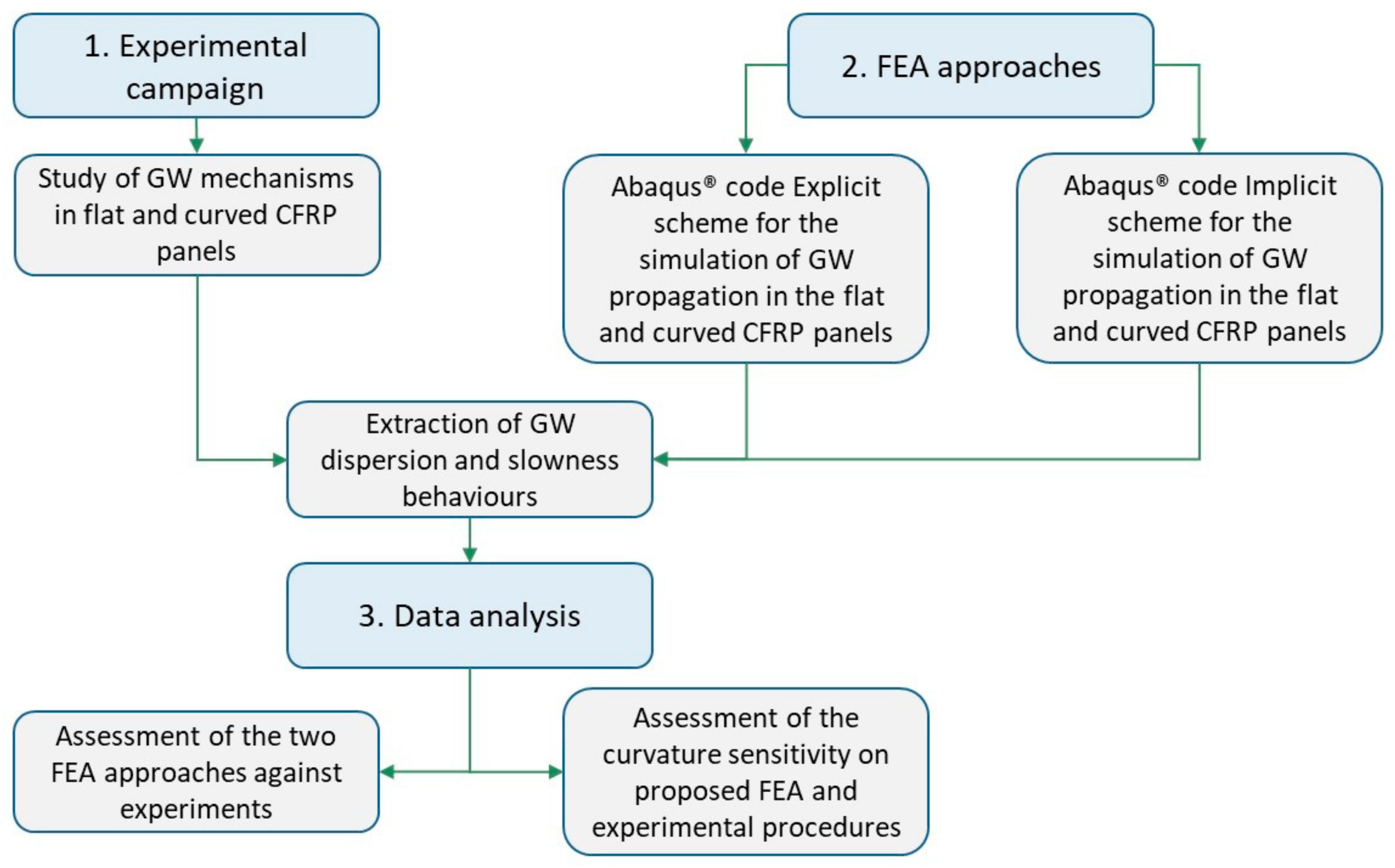
Hence, this paper aims to understand the different levels of accuracy provided by both schemes, in terms of GW propagation mechanisms and dispersion curve calculation, for cases that study a different aspect from the flat panels usually investigated in the literature. To accomplish this goal, the Abaqus/Explicit and Abaqus/Implicit software packages were used. Afterward, the predicted signals and dispersion curves extracted from the two approaches were compared with the results of an experimental campaign. Such a comparison allowed to investigate the reliability and efficiency of the numerical procedures in simulating GWs propagation. In all cases, a frequency range of from 100 kHz to 300 kHz and four different propagation directions (0°, 45°, −45°, and 90°) were investigated to highlight dispersive behavior and the slowness phenomenon, respectively. A flowchart of the research activities proposed herein is presented in Figure 1.
The remainder of the paper is organized as follows. The descriptions of the case studies and of the experimental campaign are presented in Section 2, while the modeling aspects of both numerical approaches are detailed in Section 3. Section 4 reports and discusses the results; finally, Section 5 concludes the paper.

2. Materials and Methods

This section describes the experimental campaign performed on a flat and a curved plate made from CFRP composite. The case studies, as well as the experimental equipment for the SHM application, are detailed below. The diagnostic signal’s main features are also presented.

2.1. Test Cases Overview

Both plates, made of CFRP laminates, were made up of eight laminae to a total thickness of t c   =   1.5   mm . The laminate stacking sequence is [0, 90, +45, −45]s, while the material properties of the laminae are listed in Table 1. The flat plate is square-shaped with a dimension of L   =   310   mm . The curved plate, characterized by a thickness to curvature ratio of 1:111.67, is a half-cylinder with a radius of R   =   167.5   mm . and a length of L   =   310   mm . For both panels, the 0° fiber direction is aligned along the x-axis, as shown in the schematics of Figure 2 and Figure 3.
The panels were equipped with a five-PTRT network for the SHM. For both panels, a PTRT is positioned at the center of the demonstrators. The other PTRTs are placed at a distance of h   =   84.29   mm from the edges ( 100   mm from the central one, considering this distance along the diagonals of the plates) for the flat panel, Figure 2. As regards the curved panel, this distance is verified only with respect to the two curved edges, as visible in Figure 3, whereas the intersection between the orthogonal axis of the central sensor and the orthogonal axis of any other PTRT, projected on the x-z plane, generates an angle equal to α   =   24.19 ° . The radius and thickness of the PTRT wafers are d P Z T   =   10   mm and t P Z T   =   0.25   mm , respectively. The transducer properties are listed in Table 1.

2.2. SHM Experimental Equipment and Tests

In general, the positioning of the sensors on the plate can be conducted using two strategies: either bonding to the surface or embedding into the structure [22]. In this work, the PTRTs were surface-bonded using the adhesive EA 9466 from Loctite (Henkel AG & Co. KGaA, Düsseldorf, Germany) because of the advantages in terms of manufacturing, maintenance, and replacement [2,23,24] operations. Figure 4 shows the sensors used in the experimental tests (Circular PIC255 PZT, PI Ceramic GmbH, Lindenstrasse, Germany) and the relative necessary welding, with the wires connected to the electrodes. The experimental setup for GW acquisition and sensing is reported in Figure 5 for the flat (a) and curved (b) panels. The yellow circles indicate the test case and the instruments adopted for the measurements or the test case: a Handyscope HS5 oscilloscope (TiePie Engineering) with a built-in arbitrary waveform generator, computer, probes, and connectors. The red circles represent the sensor array.
The diagnostic input signals were generated and acquired using the oscilloscope and the TiePie Multichannel program. The excitation signal was generated using the TiePie AWG waveform generator, while its parameters were defined through an in-house MATLAB routine. In particular, a Hanning windowed tone-burst signal, characterized by five cycles and a peak-to-peak amplitude equal to 12 V, was used as the excitation source. The investigated frequencies were 100, 150, 200, 250, and 300 kHz. The update frequency (a specific term for signal generation) is 4 MHz, and the number of points is 100.
The tone-burst signal, which is preferred due to the dispersive nature of Lamb waves [25], can be expressed as:
V t   =   0.5   V in   H t     H t     n f c 1     cos 2 π f c t n   sin 2 π f c t ,
where H is the Heaviside function, n is the number of cycles in the tone-burst signal, f c is the central frequency, and V in is the input amplitude.
The excitation signal is then transferred to the chosen actuator. To investigate the guided wave dispersion and slowness phenomena, PTRT 1 and PTRT 2 were chosen as actuators in the separate tests. In fact, by activating the GW signal at PTRT 1, the propagation characteristics at +45° (PTRT 2 and PTRT 5) and −45° (PTRT 3 and PTRT 4) can be extracted, while by activating the diagnostic signal at PTRT 2, a response along the 0° (PTRT 3) and 90° (PTRT 4) propagation paths can be achieved.
The TiePie digital oscilloscope was also used to record the signals acquired at the receiving sensors, according to the pitch–catch approach, with a sampling frequency of 200   MHz , resulting in a 40,000-element one-dimensional array. The total recording duration of the experimental signals was tot   =   2   ×   10 4   s , and the acquired signals from all four channels had a 12-bit resolution. The recorded data, as shown in Figure 6, were then exported and post-processed by means of a MATLAB code written by the authors for the extraction of the main signal features. Subsequently, the signals were analyzed individually.

3. Numerical Approach

Concerning numerical modeling, two different approaches have been used to model the plate and the PTRTs: the explicit (Abaqus/Explicit) and the implicit (Abaqus/Implicit) formulation schemes.
The aim of this work is to compare the explicit and implicit FEA results for the simulation of GWs. As mentioned in Section 1, although the explicit procedure is well established in the literature for simulating GWs for the unloaded configurations of the component, several problems arise when dealing with actual operating scenarios. A quasi-static load, for example, can be modeled in both schemes, although the explicit scheme hides several numerical issues that are linked to the rising internal energy of the model and to possible load-induced numerical vibrations [26]. Thus, the implicit formulation can be adopted to simulate and study the load effect on GWs with reduced effort, compared to the explicit FEA. However, before proceeding with load effects modeling on GWs, the implicit scheme must be verified and assessed for simple components under laboratory conditions (i.e., flat panels, and undamaged and unloaded configurations). To accomplish this goal, different FEAs have been developed and studied herein, as listed in Table 2.
For both modeling procedures, to reduce the number of simulations, a chirp excitation signal [7] has been used to study the dispersive behavior of GWs in the frequency band investigated in the experiments (100–300 kHz). This signal, shown in Figure 7, has an initial frequency of 80 kHz, a final frequency of 320 kHz, and a time window of 2   ×   10 4 s. A wider range is mandatory to properly reconstruct data at the boundary frequencies. All simulations have been performed with an Intel® Xeon ® Gold 6248R CPU with a total of 24 cores and 48 threads.

Explicit vs. Implicit FEA

The main differences between the explicit and implicit FEA formulations for the test cases that are analyzed herein can be detailed as follows.
In the case of the explicit FEA formulation, S4R conventional two-dimensional shell elements (having 6 degrees of freedom (DOFs) for each node) with an average element size of 2 mm were chosen for the plate, while C3D8R solid elements (characterized by 3 DOFs for each node) with an average element size of 0.5 mm were chosen for the sensors. These values allowed discretizing 8 NPW (nodes per wavelength) under 300 kHz carrier frequency. This method is conditionally stable; the time step, equal to 2.1   ×   10 7 , was chosen by considering the wave speed and the minimum element length.
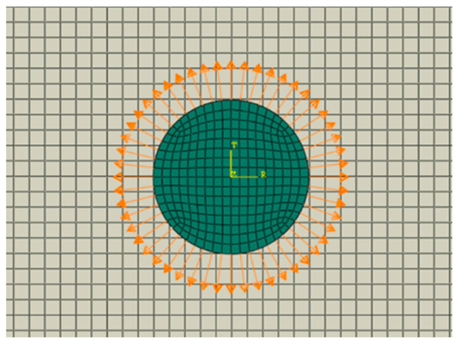
Regarding the GW propagation, radial displacements that were equivalent to the input voltage, represented by the orange-colored line in Figure 7, were calculated according to the piezoelectric relationships (the mathematical details can be found in [7]), depending on PTRT, and the plate material and geometrical properties. As shown in Figure 8, this effective radial displacement was applied to the circumference of the upper surface of the actuator, after having defined a proper polar coordinate system at its center. In terms of the computational costs, each analysis took about 10 min.
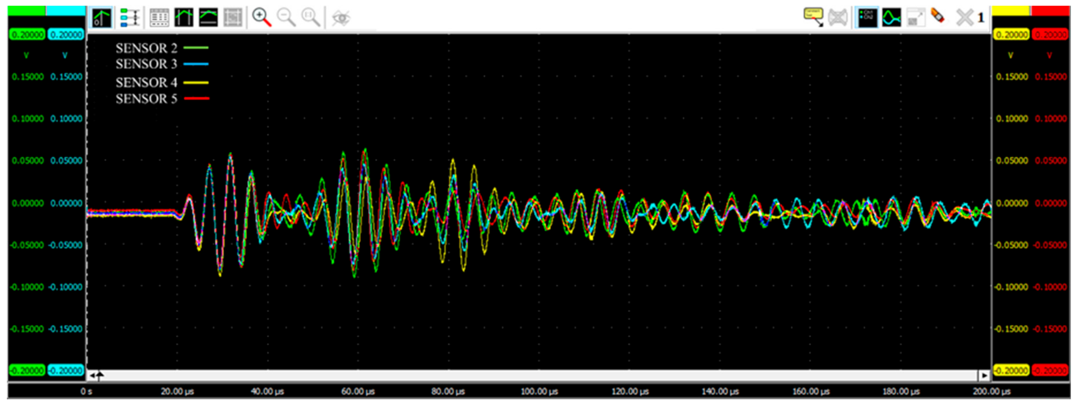
The predicted signals, recorded at the various sensor locations, were calculated as the average of the in-plane strains reads by all the nodes defining each sensor. According to the piezoelectric relationships, the voltage in PTRTs can be calculated via strain measurements, using a conversion constant for the sensing (further mathematical details can be found in [2,20]).
For the implicit formulation, C3D8I solid elements (characterized by 3 DOFs for each node) with an average element size of 2 mm were chosen for the plate, while the C3D8E solid elements (having an additional DOF related to the electrical potential with respect to the C3D8I element type, one that was not available for the explicit procedure) with an average element size of 0.5 mm were chosen for the sensors. Again, these values allowed discretizing 8 NPW, which is the minimum number required, according to the literature [13,27], at a 300 kHz carrier frequency. The C3D8E elements included the piezoelectric coupling by defining the piezoelectric coefficient and the dielectric matrices, according to the properties listed in Table 3.
The main advantage of this approach is that, differently from the explicit procedure, the diagnostic signal expressed in voltage can be directly applied to the terminals of the transducers, and the corresponding voltage response in the sensors can be directly acquired without any conversion. In detail, for the GW excitation and sensing, the signal, shown in voltage (the blue line in Figure 6), was applied at the upper surface of the actuator, while the electrical potential was imposed at 0 on the lower surface as the initial conditions (with the voltage applied along the polarization direction) [28]. For the receivers, the electrical potential had to be considered as 0 at the lower surfaces in terms of initial conditions as well, while the predicted signals in terms of voltage could be measured directly at the upper surfaces.
Although the implicit method is not as conditionally stable as the explicit one, the same maximum increment of the explicit formulation was chosen. Regarding the computational costs, each analysis took about 7 h for the implicit formulation, while only roughly 10 min of computational time was necessary for the explicit approach.
In both cases, details about the discretization of the model (Figure 9) are listed in Table 4 in terms of the number of nodes, number of elements, and characteristic element dimensions.
The adhesive bonding of the sensor array on the plates was modeled herein through the use of a node-to-surface contact formulation, employing “tie” interfaces at the contact surfaces. Finally, the four corners of the plates were constrained.
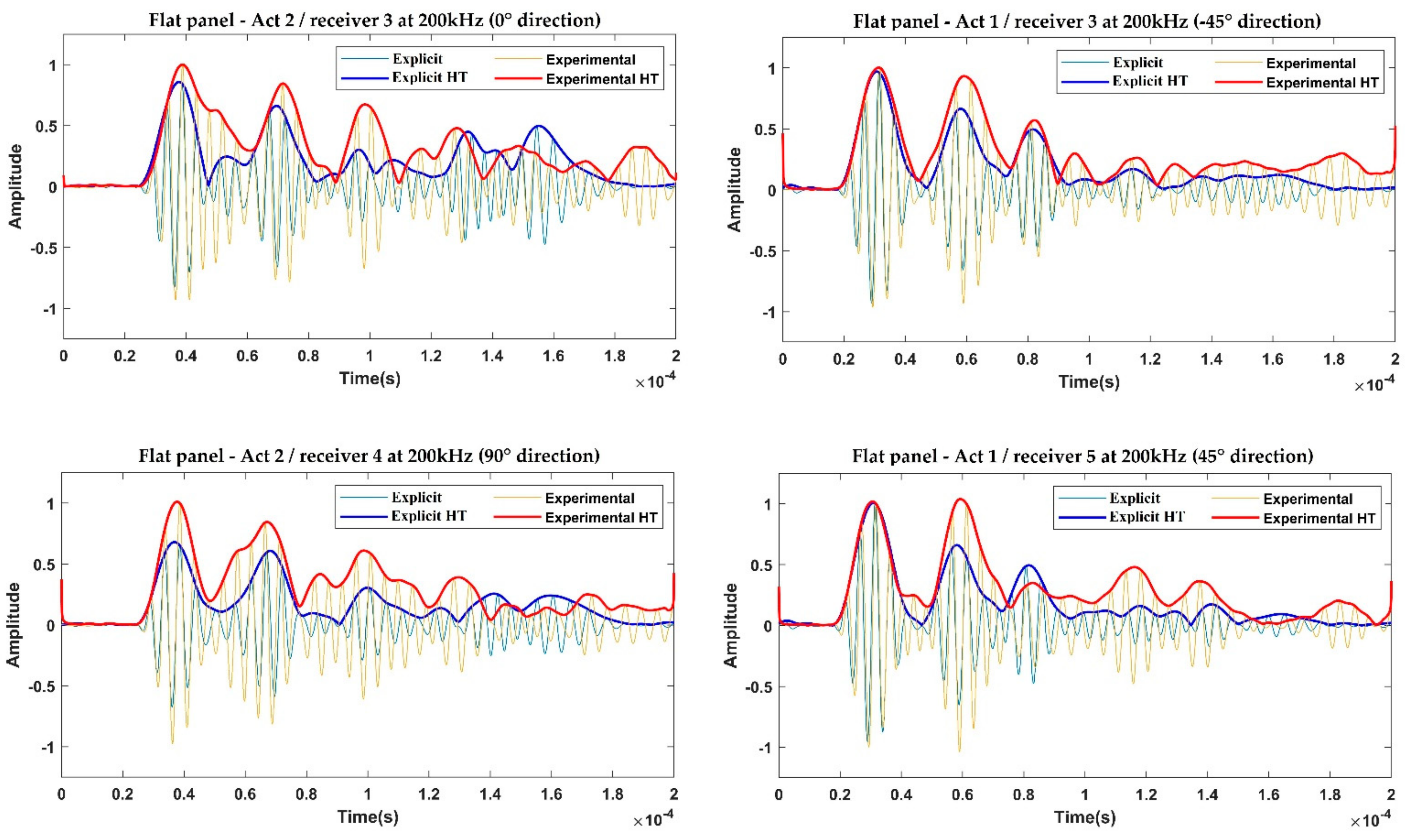
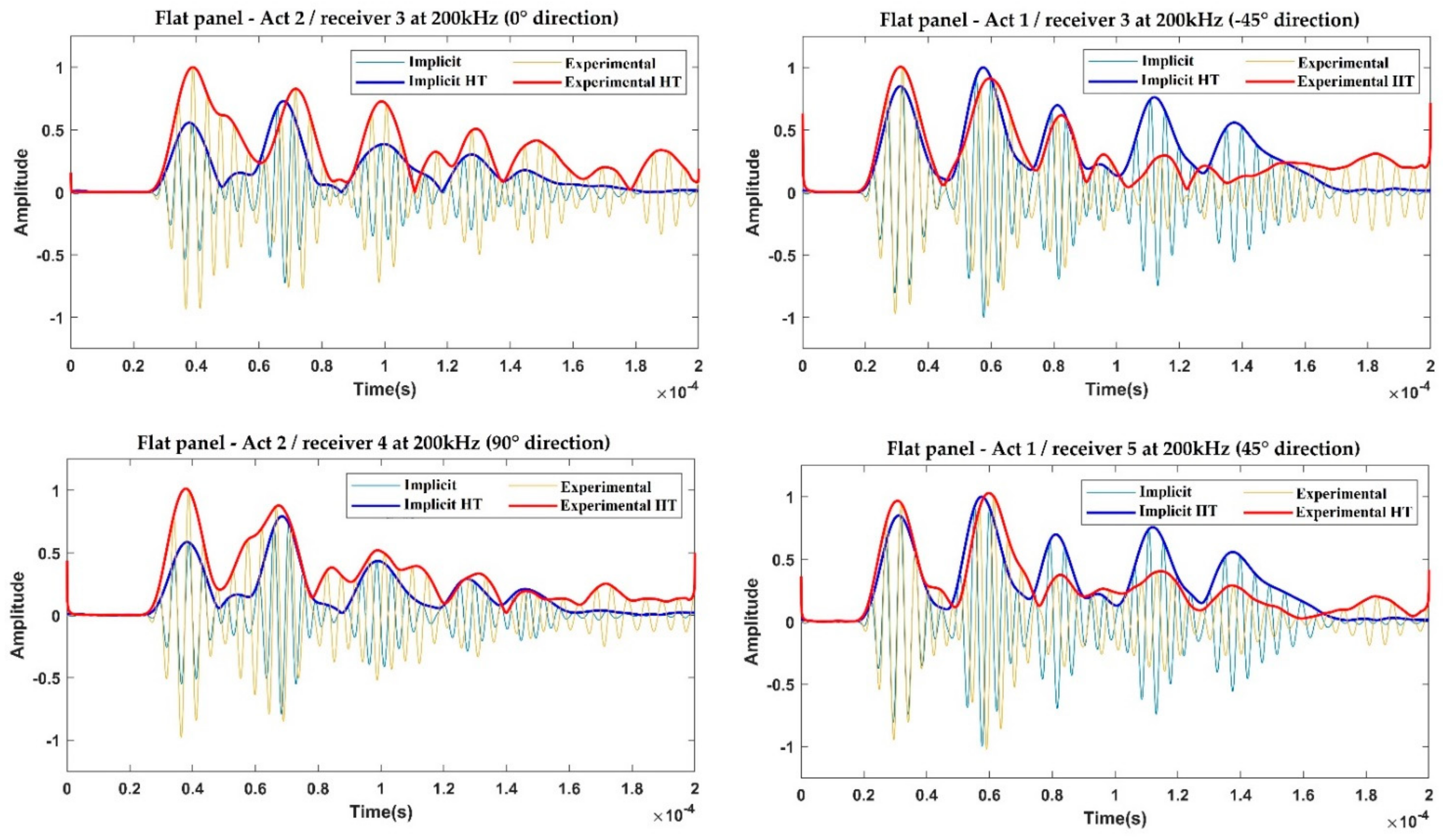
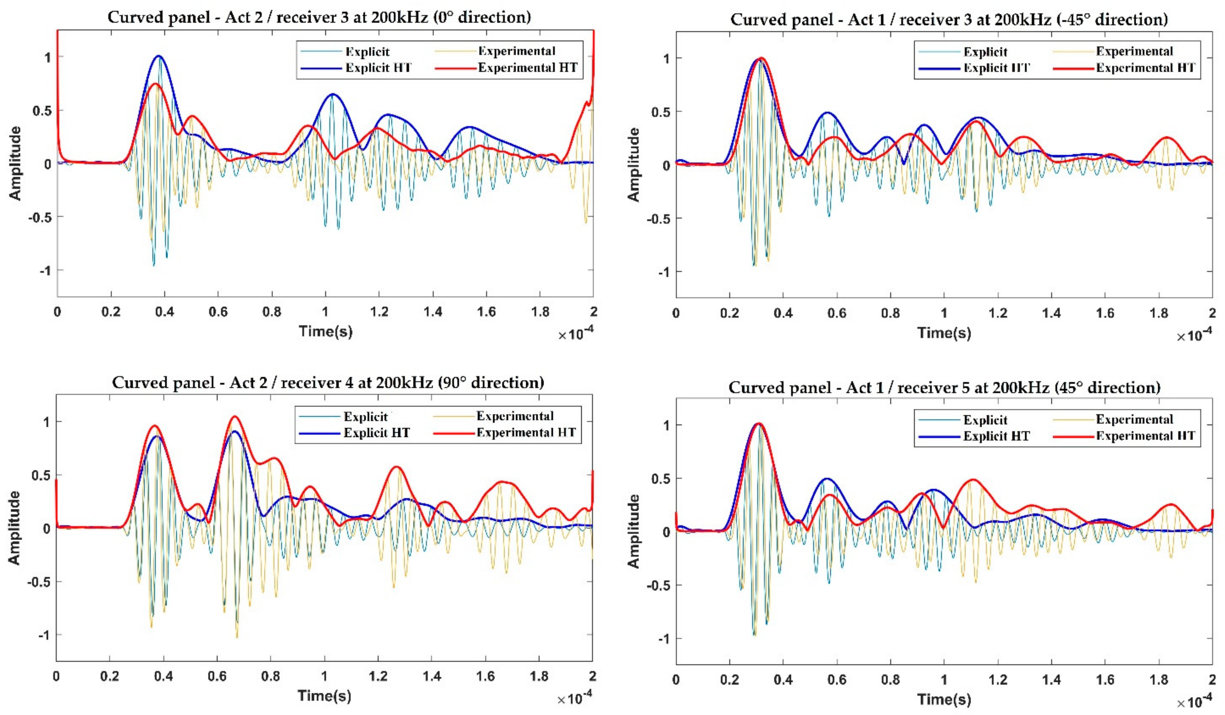
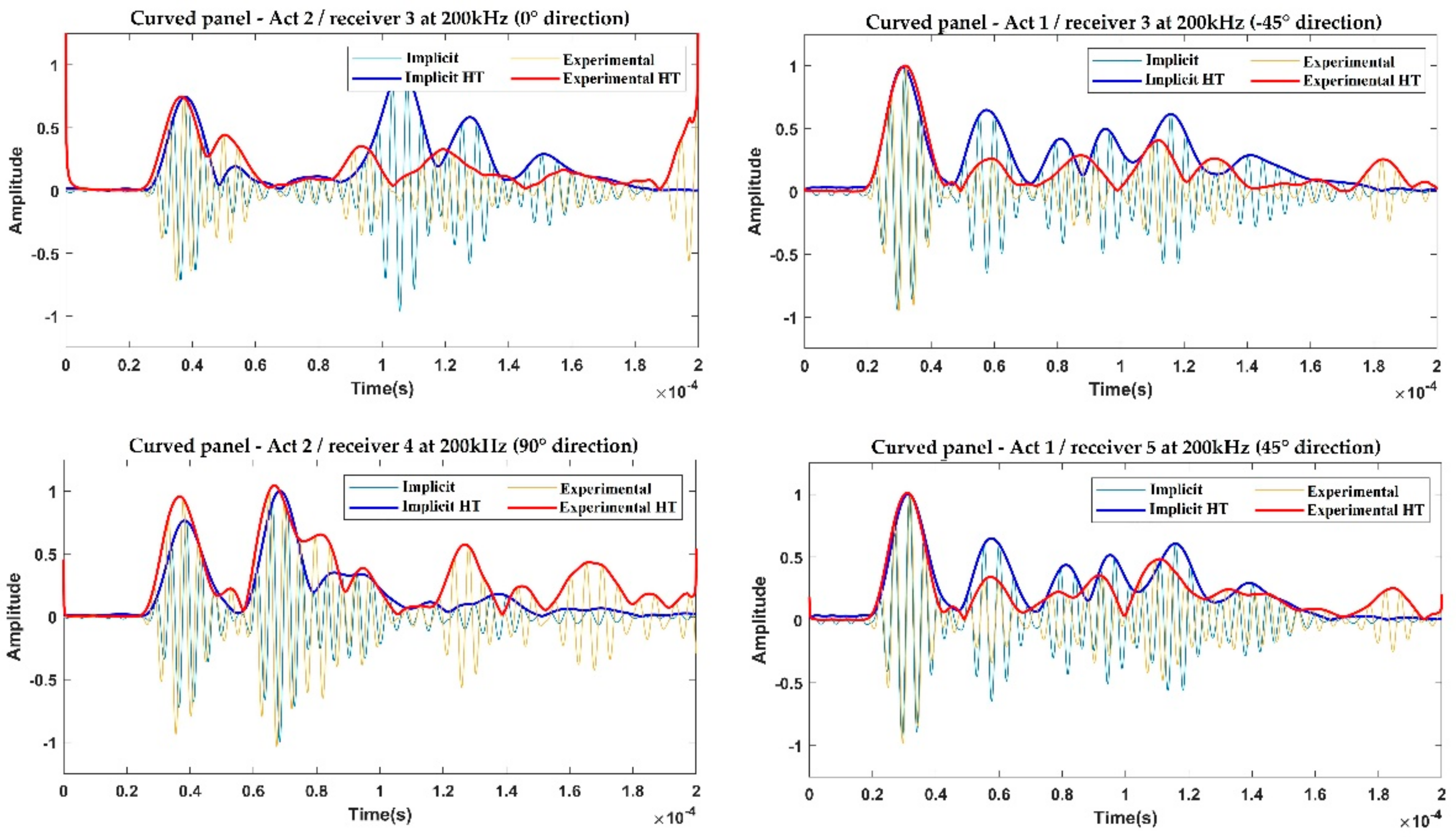
Then, signals were processed by means of the developed code. In particular, recorded data were reconstructed in n-cycles, using sinusoidal tone-burst Hanning-windowed signals from 100 kHz to 300 kHz, with a step of 50 kHz, using the reconstruction procedure described in [29]. The reconstruction phase in the tone-burst response is fundamental to enabling the representation of the signals in the time domain (because of the dispersive nature of GWs [25]), and the GW group velocities extraction for each carrier frequency.
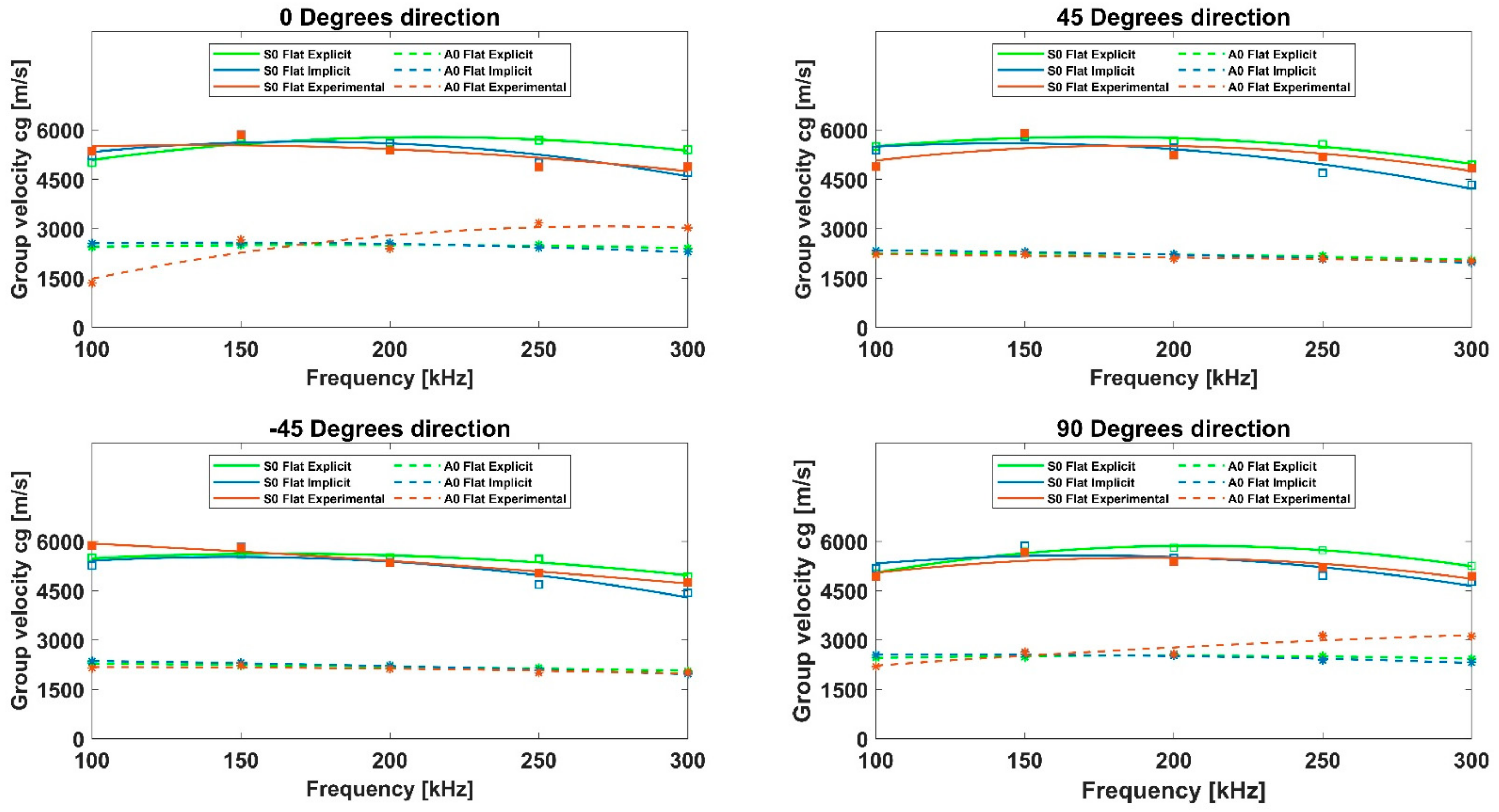
Thus, the numerical results and experimental data are compared, in terms of amplitudes and dispersion curves.

4. Results and Analysis

In this section, the results obtained from both approaches and both panels are compared. Overall, the total number of analyzed signals is 120. This value is equal to a   ×   f   ×   d   ×   n , where a is the number of approaches used for this acquisition (3), f is the number of considered frequencies (5), d is the number of investigated propagation paths (4), and n is the number of panels investigated (2). First, the numerical data extracted from the two formulation schemes were compared to experimental ones. For the sake of clarity and conciseness, the analysis of the results is reported here only for those signals reconstructed under a 200 kHz carrier. Then, the dispersion curves for both FEA approaches were compared to experiments for the d directions. The characteristic directions under consideration are reported in Table 5.

4.1. Numerical Analyses vs. Experiments

The results are shown for each propagation direction, according to the sensor disposition and the composite layout. Figure 10 and Figure 11 show the comparison between the experimental data and the explicit and implicit approaches, respectively, for the flat panel (200 kHz carrier).
Figure 12 and Figure 13 report the same examples but refer to the curved panel (200 kHz carrier).
As is visible from these figures, both the explicit and implicit predicted signals match the experimental trends very well, especially for the 0-order wave modes, in terms of propagation velocities and time of arrival (which comprise the information needed to correctly capture the dispersion and slowness phenomena). Such a result is better appreciated by analyzing the envelopes of the signals, obtained using the Hilbert transform (HT) method. The satisfactory level of accuracy allows us to consider that both approaches have been validated, first with respect to the signal phases, then with respect to the propagation velocities of the S0 and A0 modes.
Then, the dispersion curves were extracted for both panels. The developed MATLAB® code automatically extracted the time of flight (ToF) of the 0-order wave packets ( S 0 and A 0 ) from the HT envelopes. By knowing the transducers’ position, the wave group velocities ( c g ) of the S 0 and A 0 GW packets were easily calculated. Figure 14 and Figure 15 report the comparison of the two numerical approaches, in terms of both dispersion and slowness phenomena, against the experimental data for the flat and curved panels, respectively. The S 0 wave mode is represented by the solid lines, while the A 0 mode is represented by the dotted lines. The separate colors are part of the specific approach. For both plates, the two numerical approaches provided coherent results when compared with the experiments. Consequently, the explicit method turned out to be preferable, due to the generally lower computational costs. However, if the objective was to study the GW propagation in the loaded configuration of the panel, which was representative of an operating scenario, the implicit formulation can be adopted as well. As mentioned in Section 1, once validated, this approach can simplify the modeling of the load. In fact, for the modeling of a quasi-static load under the explicit scheme, several efforts are needed: an explicit quasi-static approach must be properly defined, to reduce the inertia forces and the raising load-induced kinetic energy of the model [28]. For all these reasons, an implicit scheme should be preferred for easier modeling, despite the higher computational costs.

4.2. Curvature Effect of GW

Subsequently, in order to verify the effects of the curvature of the structure on GW propagation, the dispersion curves extracted from the two numerical approaches and the experiments for both flat and curved panels were compared. Figure 16 reports the dispersion curves for the flat and curved panels extracted from the experiments, while Figure 17 and Figure 18 show the same comparisons for the data extracted from the numerical explicit and numerical implicit formulations, respectively.
According to the results provided in the literature [9,10] and by analyzing Figure 16, Figure 17 and Figure 18, for such a low thickness-to-radius ratio (1: 111.67), the group velocities of the A 0 and S 0 modes extracted from the curved panel almost coincided with the flat ones for all cases. In particular, the results from the two panel configurations highlight a better match between the dispersion curve trends in the numerical approaches, while the experimental data showed a slight mismatch in the two geometrical configurations (see the change in the curve trends in Figure 16). This result could, however, be justified due to the slight mismatch in the positioning of the transducers on the curved panel, in terms of both location and adhesion.

5. Conclusions

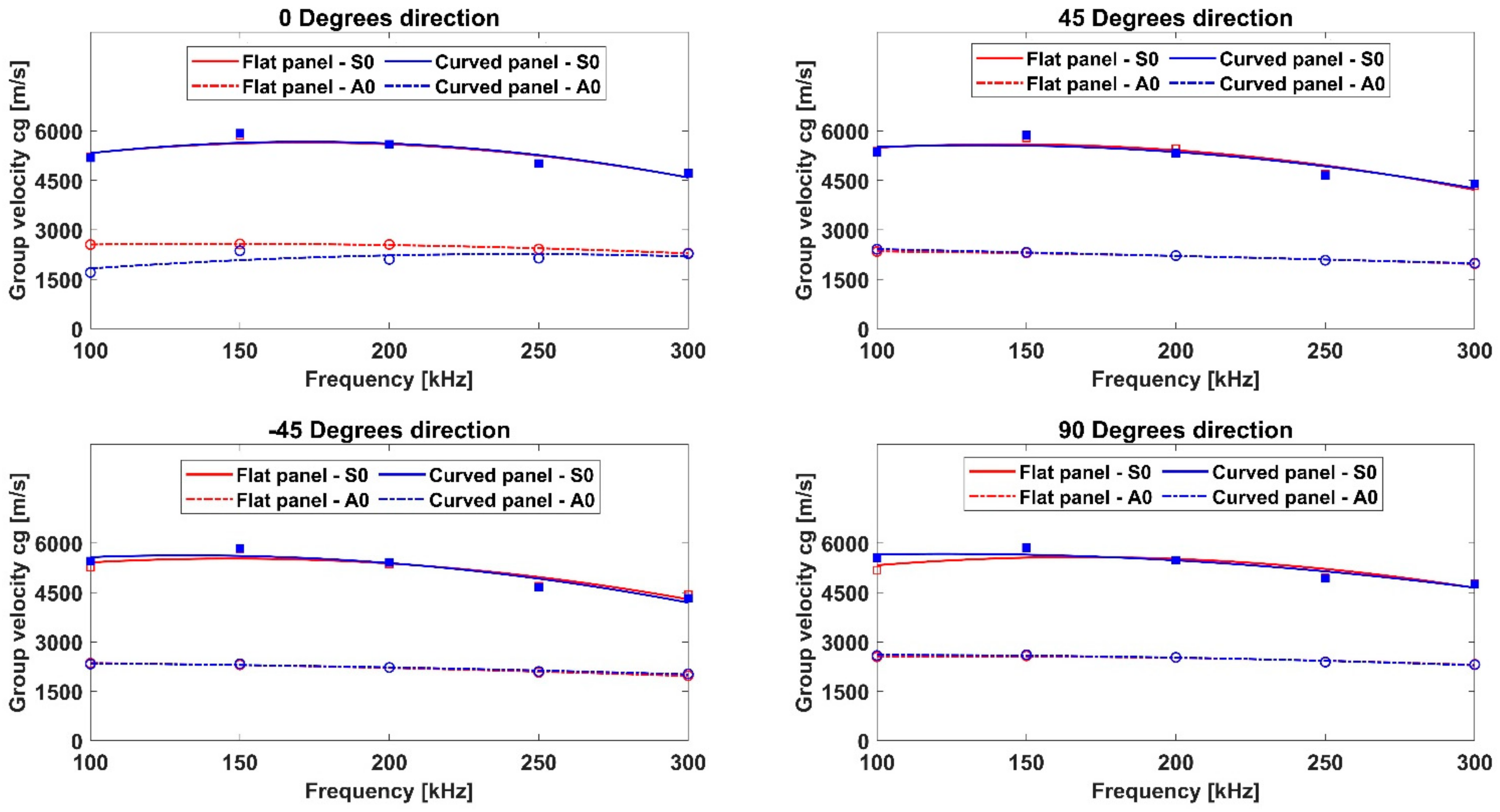
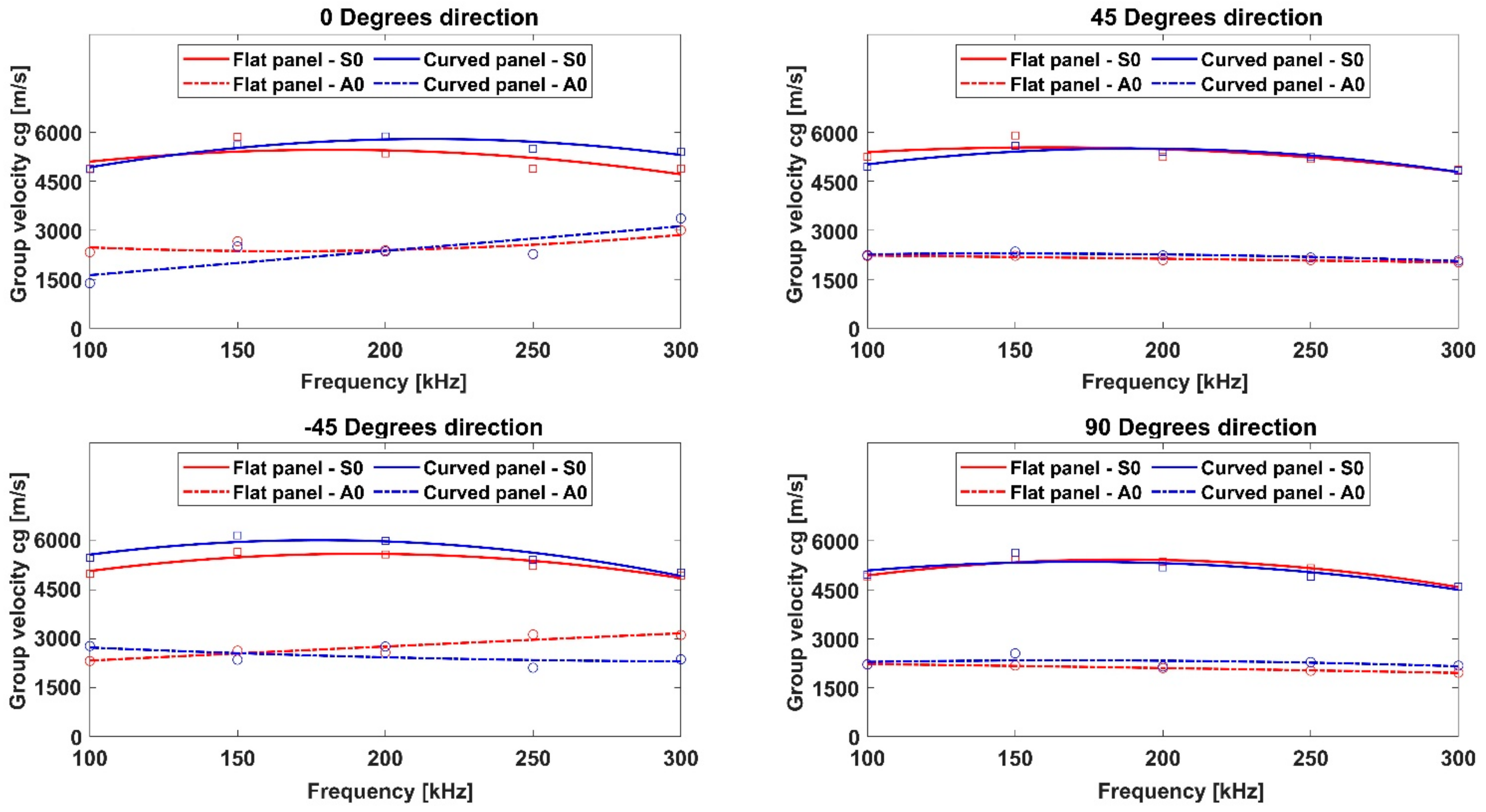
In this paper, numerical and experimental investigations into two CFRP composite components, a flat and a curved panel, were carried out to study the GW propagation mechanisms.
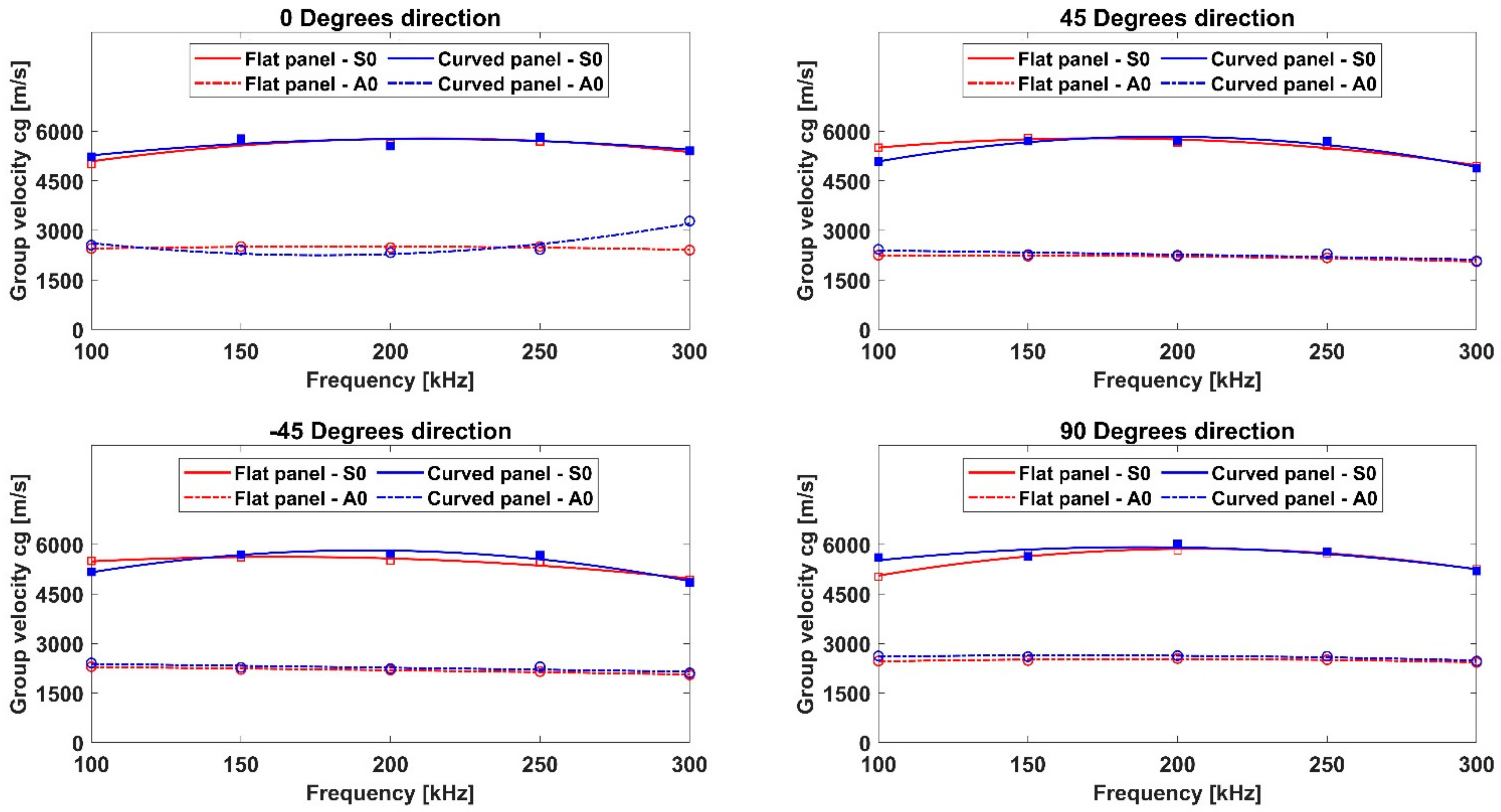
Two finite element modeling approaches, based on implicit and explicit formulations, respectively, were investigated. An experimental campaign was also carried out. The predicted measures, in terms of the recorded signals and GW dispersion curves, were compared against the experimental dataset in order to assess and validate the numerical procedures, also comparing those for curved panels. The results were extracted for both geometrical configurations in a specific frequency range, 100–300 kHz, which is characteristic of non-destructive testing techniques. The numerical and experimental dispersion curves were extracted to highlight and compare the performance of the two numerical approaches. Moreover, the dispersion curves for both flat and curved panels, extracted by the experiments as well as by both implicit and explicit schemes, were respectively compared to highlight the different curvature sensitivity of the three approaches. The results comparison allowed to assess the reliability of the different modeling approaches when modeling GW propagation phenomena (dispersion and slowness). Specifically, it was proved that even if both numerical formulation schemes can provide accurate results with respect to the experimental data for both panel configurations, the explicit FEA model is in fact preferable, due to the considerably reduced computational costs. This aspect is fundamental for properly modeling GW propagation in real in-service scenarios, for example, under quasi-static loading conditions, for which an implicit FEA should be instead preferred despite the higher computational costs.
Furthermore, for the curved panel, which was characterized by a thickness-to-curvature radius of 1:111.67, the propagation speeds (for varying propagation paths) of the S 0 and A 0 modes are quite similar to those registered in the flat configuration of the panel. This result agrees with the literature. A better match between the dispersion curve trends for the numerical approaches was found for the investigated configurations, while the experimental data showed a slight mismatch. This result could, however, be justified due to the slight mismatch in the positioning of the transducers on the curved panel, in terms of both location and adhesion.
This work represents the basis for the next research activity steps, which will involve a study of the load effect on GW propagation mechanisms in curved FRP composite engineering structures, for the assessment of SHM system damage sensitivity.

Author Contributions

Conceptualization, A.D.L. and D.P.; formal analysis, D.P., A.P. and A.A.; funding acquisition, A.D.L.; investigation, A.D.L. and D.P.; methodology, A.D.L., D.P., A.P. and A.A.; project administration, A.D.L.; supervision, F.C.; validation, D.P. and F.C.; writing—review and editing, A.D.L., D.P., A.P., A.A. and F.C. All authors have read and agreed to the published version of the manuscript.

Funding

This research was funded by the University of Campania’s “Luigi Vanvitelli” in the framework of the “SAFES—Smart Patch for Active Shm” funded research project, as part of the VALERE 2020 program.

Institutional Review Board Statement

Not applicable.

Informed Consent Statement

Not applicable.

Data Availability Statement

The data presented in this study are available on request from the corresponding author.

Conflicts of Interest

The authors declare no conflict of interest.

Abbreviations

CFRPCarbon fiber-reinforced plastic
CIEDACombined implicit-explicit dynamic analysis
CgGroup velocity
DOFDegrees of freedom
EDAExplicit dynamic analysis
EOCsOperating loading and environmental conditions
FEAFinite element analysis
GWGuided wave
IDAImplicit dynamic analysis method
PTRTPiezoelectric transmitter/receiver transducer
SHMStructural health monitoring
ToFTime of flight

References

  1. Rose, J.L. A Baseline and Vision of Ultrasonic Guided Wave Inspection Potential. J. Press. Vessel Technol. 2002, 124, 273–282. [Google Scholar] [CrossRef]
  2. Su, Z.; Ye, L. Identification of Damage Using Lamb Waves; Pfeiffer, F., Wriggers, P., Eds.; Lecture Notes in Applied and Computational Mechanics; Springer: London, UK, 2009; Volume 48, ISBN 978-1-84882-783-7. [Google Scholar]
  3. Rocha, H.; Semprimoschnig, C.; Nunes, J.P. Sensors for Process and Structural Health Monitoring of Aerospace Composites: A Review. Eng. Struct. 2021, 237, 112231. [Google Scholar] [CrossRef]
  4. Gorgin, R.; Luo, Y.; Wu, Z. Environmental and Operational Conditions Effects on Lamb Wave Based Structural Health Monitoring Systems: A Review. Ultrasonics 2020, 105, 106114. [Google Scholar] [CrossRef]
  5. Wilcox, P.D. A Rapid Signal Processing Technique to Remove the Effect of Dispersion from Guided Wave Signals. IEEE Trans. Ultrason. Ferroelectr. Freq. Control. 2003, 50, 419–427. [Google Scholar] [CrossRef] [PubMed]
  6. Memmolo, V.; Monaco, E.; Boffa, N.D.; Maio, L.; Ricci, F. Guided Wave Propagation and Scattering for Structural Health Monitoring of Stiffened Composites. Compos. Struct. 2018, 184, 568–580. [Google Scholar] [CrossRef]
  7. De Luca, A.; Perfetto, D.; Lamanna, G.; Aversano, A.; Caputo, F. Numerical Investigation on Guided Waves Dispersion and Scattering Phenomena in Stiffened Panels. Materials 2021, 15, 74. [Google Scholar] [CrossRef] [PubMed]
  8. YU, Z.; XU, C.; SUN, J.; DU, F. Guided Wave Propagation Analysis in Stiffened Panel Using Time-Domain Spectral Finite Element Method. Chin. J. Aeronaut. 2021. [Google Scholar] [CrossRef]
  9. Wilcox, P.D. Lamb Wave Inspection of Large Structures Using Permanently Attached Transducers. Ph.D. Dissertation, Imperial College London (University of London), London, UK, 1998. [Google Scholar]
  10. Fong, K.L.J. A Study of Curvature Effects on Guided Elastic Waves. Ph.D. Dissertation, Imperial College London (University of London), London, UK, 2005. [Google Scholar]
  11. Santana, G.A.; Malekan, M.; Araújo, A.M.; Donadon, L.V.; Cimini, C.A., Jr. Finite Element Evaluation of the Effects of Curvature in Lamb Waves for Composites Structural Health Monitoring. Lat. Am. J. Solids Struct. 2018, 15, 1–21. [Google Scholar] [CrossRef]
  12. De Luca, A.; Perfetto, D.; De Fenza, A.; Petrone, G.; Caputo, F. Guided Wave SHM System for Damage Detection in Complex Composite Structure. Theor. Appl. Fract. Mech. 2020, 105, 102408. [Google Scholar] [CrossRef]
  13. De Luca, A.; Perfetto, D.; De Fenza, A.; Petrone, G.; Caputo, F. Guided Waves in a Composite Winglet Structure: Numerical and Experimental Investigations. Compos. Struct. 2019, 210, 96–108. [Google Scholar] [CrossRef]
  14. Wang, T. Finite Element Modelling and Simulation of Guided Wave Propagation in Steel Structural Members. Ph.D. Dissertation, University of Western Sydney, Penrith, Australia, 2014. [Google Scholar]
  15. Leckey, C.A.C.; Wheeler, K.R.; Hafiychuk, V.N.; Hafiychuk, H.; Timuçin, D.A. Simulation of Guided-Wave Ultrasound Propagation in Composite Laminates: Benchmark Comparisons of Numerical Codes and Experiment. Ultrasonics 2018, 84, 187–200. [Google Scholar] [CrossRef]
  16. Markovic, N.; Stojic, D.; Cvetkovic, R.; Radojicic, V.; Conic, S. Numerical Modeling of Ultrasonic Wave Propagation-by Using of Explicit FEM in ABAQUS. Facta Univ. Ser. Archit. Civ. Eng. 2018, 16, 135–147. [Google Scholar] [CrossRef]
  17. Lee, Y.F.; Lu, Y. Advanced Numerical Simulations Considering Crack Orientation for Fatigue Damage Quantification Using Nonlinear Guided Waves. Ultrasonics 2022, 124, 106738. [Google Scholar] [CrossRef]
  18. Zhang, B.; Sun, X.C.; Eaton, M.J.; Marks, R.; Clarke, A.; Featherston, C.A.; Kawashita, L.F.; Hallett, S.R. An Integrated Numerical Model for Investigating Guided Waves in Impact-Damaged Composite Laminates. Compos. Struct. 2017, 176, 945–960. [Google Scholar] [CrossRef] [Green Version]
  19. Maio, L.; Fromme, P. On Ultrasound Propagation in Composite Laminates: Advances in Numerical Simulation. Prog. Aerosp. Sci. 2022, 129, 100791. [Google Scholar] [CrossRef]
  20. Perfetto, D.; De Luca, A.; Perfetto, M.; Lamanna, G.; Caputo, F. Damage Detection in Flat Panels by Guided Waves Based Artificial Neural Network Trained through Finite Element Method. Materials 2021, 14, 7602. [Google Scholar] [CrossRef]
  21. De Luca, A.; Perfetto, D.; Caputo, F.; Petrone, G.; De Fenza, A. Numerical Simulation of Guided Waves Propagation in Loaded Composite Structures. AIP Conf. Proc. 2020, 2309, 020029. [Google Scholar]
  22. Paget, C.A. Active Health Monitoring of Aerospace Composite Structures by Embedded Piezoceramic Transducers. Ph.D. Dissertation, Institutionen för Flygteknik, Ljungbyhed, Sweden, 2001. [Google Scholar]
  23. Kessler, S.S.; Spearing, S.M.; Soutis, C. Damage Detection in Composite Materials Using Lamb Wave Methods. Smart Mater. Struct. 2002, 11, 269–278. [Google Scholar] [CrossRef] [Green Version]
  24. Bhalla, S.; Soh, C.K.; Liu, Z. Wave Propagation Approach for NDE Using Surface Bonded Piezoceramics. NDT E Int. 2005, 38, 143–150. [Google Scholar] [CrossRef]
  25. Giurgiutiu, V. Structural Health Monitoring with Piezoelectric Wafer Active Sensors, 2nd ed.; Elsevier: Amsterdam, The Netherlands, 2006; ISBN 1932078576. [Google Scholar]
  26. De Luca, A.; Caputo, F.; Sharif Khodaei, Z.; Aliabadi, M.H. Damage Characterization of Composite Plates under Low Velocity Impact Using Ultrasonic Guided Waves. Compos. Part B Eng. 2018, 138, 168–180. [Google Scholar] [CrossRef]
  27. Sharif-Khodaei, Z.; Aliabadi, M.H. Assessment of Delay-and-Sum Algorithms for Damage Detection in Aluminium and Composite Plates. Smart Mater. Struct. 2014, 23, 075007. [Google Scholar] [CrossRef]
  28. Dassault Systems Simulia Corp Abaqus 6.14 Analysis User’s Guide 2014. Available online: http://130.149.89.49:2080/v6.14/pdf_books/CAE.pdf (accessed on 1 April 2022).
  29. Dafydd, I.; Sharif Khodaei, Z. Analysis of Barely Visible Impact Damage Severity with Ultrasonic Guided Lamb Waves. Struct. Health Monit. 2020, 19, 1104–1122. [Google Scholar] [CrossRef]
Figure 1. Flowchart of the research activities.
Sustainability 14 06924 g001
Figure 2. Schematic of the geometry and PTRTs network for the flat panel.
Sustainability 14 06924 g002
Figure 3. Schematic of the geometry and PTRTs network for the curved panel. (a) Front view. (b) Top view.
Sustainability 14 06924 g003
Figure 4. (a) PIC255 sensors, as used in the experimental tests. (b) Relative welding, with the wires connected to the electrodes.
Sustainability 14 06924 g004
Figure 5. Experimental setup for the (a) flat and (b) curved panels, with five surface-mounted sensors (numbered from 1 to 5 in the red circles). The yellow circles refer to (1) the flat and curved plates, (2) the oscilloscope, (3) the computer, (4) the probes, and (5) the connectors.
Sustainability 14 06924 g005
Figure 6. An example of an experimental acquired data set, considering the actuator in position PTRT 1.
Sustainability 14 06924 g006
Figure 7. Actuator input for numerical investigations for the implicit (blue line) and explicit (orange line) formulations.
Sustainability 14 06924 g007
Figure 8. An explicit FEA–GW excitation signal, modeled by applying an equivalent radial displacement field on the upper actuator edge.
Sustainability 14 06924 g008
Figure 9. FE models of the (a) flat and (b) curved panels.
Sustainability 14 06924 g009
Figure 10. Comparison between the explicit FEA and the experimental acquisitions on the flat panel for the investigated propagation paths—200 kHz.
Sustainability 14 06924 g010
Figure 11. Comparison between the implicit FEA and the experimental acquisitions on the flat panel for the investigated propagation paths—200 kHz.
Sustainability 14 06924 g011
Figure 12. Comparison between the explicit FEA and the experimental acquisitions on the curved panel for the investigated propagation paths—200 kHz.
Sustainability 14 06924 g012
Figure 13. Comparison between the implicit FEA and the experimental acquisitions on the curved panel for the investigated propagation paths—200 kHz.
Sustainability 14 06924 g013
Figure 14. Dispersion curves of the S 0   and A 0 mode group velocities propagating in the flat panel, evaluated with the explicit approach (in green), the implicit approach (in blue), and the experiments (in red).
Sustainability 14 06924 g014
Figure 15. Dispersion curves of the S 0 and A 0 mode group velocities on the curved panel, evaluated with the explicit approach (in green), the implicit approach (in blue), and the experiments (in red).
Sustainability 14 06924 g015
Figure 16. Comparison of the S 0 and A 0 mode dispersion curves for the flat panel (in red) and the curved panel (in blue)—experiments.
Sustainability 14 06924 g016
Figure 17. Comparison of the S 0 and A 0 modes dispersion curves on the flat panel (in red) and the curved panel (in blue)—explicit FEA.
Sustainability 14 06924 g017
Figure 18. Comparison of the S 0 and A 0 dispersion curves on the flat panel (in red) and the curved panel (in blue)—implicit FEA.
Sustainability 14 06924 g018
Table 1. Material mechanical properties of the CFRP composite lamina and PIC255 PTRTs.
Material PropertySymbolUnitsCFRP LaminaPTRT
Mass density ρ kg   m 3 1534 7800
Longitudinal Young’s modulus E 11 GPa 123.182 62.1
Transversal Young’s modulus E 22 GPa 7.700 62.1
E 33 7.700 48.3
Shear modulus G 12 GPa 3.60 23.5
G 13 3.60 21
G 23 2.70 21
Poisson’s ratio ν 12 0.360 0.32
ν 13 0.360 0.44
ν 23 0.4 0.44
Table 2. Case studies overview.
Case StudiesFEA TypeActuator
Flat panelExplicit, ImplicitPTRT 1, PTRT 2
Curved panelExplicit, ImplicitPTRT 1, PTRT 2
Table 3. The PIC255 dielectric and electromechanical properties adopted in the implicit FEA.
Material PropertySymbolUnitsValue
Dielectric constant K 3 1280
Dielectric permittivity at constant strain ε 11   =   ε 22 nF   m 1 8.245
ε 33 7.122
Piezoelectric strain
coefficients
d 31 pC   N 1 180
d 33 400
d 15 550
Table 4. FE model details for the implicit and explicit FEA formulations, with reference to the case studies—8 NPW under a 300 kHz carrier.
ApproachPanel ShapeComponentElement TypeNumber
of Nodes
Number
of Elements
Average
Element Size (mm)
ExplicitFlatPlateS4R25,29125,6002
PTRTC3D8R12517680.5
CurvedPlateS4R41,18440,7652
PTRTC3D8R12787960.5
ImplicitFlatPlateC3D8I48,67224,0252
PTRTC3D8E12517680.5
CurvedPlateC3D8I82,36840,7652
PTRTC3D8E12787960.5
Table 5. Investigated paths for the definition of the dispersion curves.
Measurement DirectionActuatorReceiver
45°PTRT 1PTRT 2
−45°PTRT 1PTRT 3
PTRT 2PTRT 3
90°PTRT 2PTRT 4
Publisher’s Note: MDPI stays neutral with regard to jurisdictional claims in published maps and institutional affiliations.

