Scenario-Based Predictions of Urban Dynamics in Île-de-France Region: A New Combinatory Methodologic Approach of Variance Analysis and Frequency Ratio

Abstract

Modelling land use dynamics is a critical scientific issue. Despite a diversity of models coming from the fields of remote sensing, geography, and economics, including multicriteria decision analysis and machine-learning models, taking into account the external driving factors of urbanization is still a main challenge. This study aims at simulating various land use development scenarios with global and local parameters. Thus, the developed approach is able to estimate and simulate the dynamic evolution of land use classes, the evolution of urban attractivity, both of which depend on several driving factors. The proposed scenarios incorporate anticipated global changes, such as an increase in oil prices and a decrease in wealth, and local spatial changes such as the provision of new rail lines and the development of new activity zones. The results of simulations, for the study area covering a great part of the Île-de-France region, show for the year 2050 an 18% increase in urban areas and a 25% decrease in bare soils, compared to the year 2018. Moreover, the increase of global prices and the reduction of income levels would increase the attractivity of public transport modes and drive urbanization around stations, reduce the accessible distances to public transport systems by 8.5%, reduce the dependency on private vehicles, and increase the concentrated saturation of urban development. These scenarios will serve as a basis for the deployment of nature-based solutions and renewable energy production.

1. Introduction

Within the last 30 years, the models for the prediction of land use dynamics have become a critical scientific issue with questions about their accuracy, structure, ability for improvement by combining them with other models [1,2], and their ability to cover a wide array of land use scenarios depending on several factors [1]. The complex interactions of urban growth with its surrounding with respect to socio-economic and environmental contexts represent an emerging issue to be evaluated and examined continuously. For instance, deforestation and the loss of green lands in addition to the pollution problems and non-controllable population growth is a dynamic problem whose study requires simulating urban growth and anticipating the evolution of the corresponding human activities [3,4]. The importance of predicting land use changes could be perceived as the need to have a vision for future land changes, mainly as a result of social and economic activities, in order to plan accurately the provisions of urban and infrastructural services, to control the extensive urbanization in a sustainable form, and to mitigate the negative risks resulting from these changes [5].

1.1. Review of Existing Models

Moreover, simulating the impacts of policies on spatial evolution can be helpful for local decision-makers. For this purpose, different models were developed to represent the future changes by employing the simulations of equation models [6]. Indeed, land use evolution is mainly a spatial problem, requiring techniques able to cope with this dimension, but depends also on non-spatial factors such as the evolution of technologies. Some of the models focus mainly on the spatial dimension of the simulation (generally with the formalism of Cellular Automata (CA)); others draw more attention to estimate the transitions between land use classes, whatever their locations (generally with Markov Chain Models (MCM). Most models couple these two approaches. For instance, operational models such as “Slope, Land cover, Excluded regions, Urban land cover, Transportation, and Hill shade model (SLEUTH)”, “Conversion of Land Use and its Effects (CLUE)”, and the Cellular Automata Markov Chain Models (CA-MCM) prediction model, mostly conducted in TerrSet software, couple and extend the CA and MCM paradigms. These models were employed in different studies for China [7,8,9], Lebanon [10,11], Libya [12], India [13], and Portugal [14]. It is worth noting that these models are only spatial and are unable to include the socio-economic factors within the simulations process.

However, investigating and taking into account the projection of population growth as well as the possible socio-economic, environmental, infrastructural, planning and strategic scenarios, is considered a key factor for predicting the future land use and urban dynamics [1,2,15]. These authors also indicated that the physical and soil aspects of the study area in addition to the previous land use/land cover (LULC) distribution could also affect the future dynamics. These limitations of the dynamics models were overpassed in some studies by combining Multi-Criteria Analysis (MCA) techniques for additional socio-economic, physical and infrastructural factors (generating suitability maps), with the simulation processes. Examples of these studies, that combine the CA-based models as SLEUTH with the multi-criteria decision techniques as the Analytical Hierarchy Process (AHP), can be found in [16,17,18,19,20].

Moreover, some studies [21,22] employed the bottom-up technique of the Agent-Based Models (ABM) in combination with the MCA methods and the CAMCM models to predict future urban development. The ABM designed for the indicated studies take into consideration the maximization of utility for three classes of agents: real estate developers, residents, and the government. For each of these agents, the maximization of the profitability/utility is specific. For instance, real estate developers seek to increase their investments’ profits by looking for locations increasing the housing prices and decreasing costs in addition to land price. The profitability is calculated with the help of rasterized data of land price, construction costs, and housing prices at the pixel/cell level. Similarly, residents follow a preference-driven agenda and look for balancing the housing prices with the sought-after accessibilities to socio-economic activities, infrastructure, and other services in order to maximize their utility of residence’s location. In contrast, the government and local authority try to achieve sustainable development and preserve natural areas by restraining constructions in different zones through policies. However, this type of model is mainly based on the involvement of land use knowledge and experience [23] which could, to some extent, be considered biased by personal subjectivity.

Similarly, other statistical models such as frequency ratio, logistic regression, and weights of evidence models were also combined with the dynamics model to integrate the aforementioned driving factors as in recent studies [20,24,25,26,27]. However, the Machine Learning (ML) models combined with dynamic ones are generally preferred and found to be more accurate than statistical methods [2].

In a further elaborated way, ML models can be used to guide, by calibration, the transition rules and generate probability maps in the course of the simulations based on socio-economic and environmental factors, strategic data, infrastructures, accessibility, and topography [15]. The commonly used ML models are Artificial Neural Networks (often Multi-Layer Perceptron), the K-nearest-neighbor, and the Decision Trees. Spatial growth models incorporating ML techniques were used in studies during the last 10 years [15,28,29,30,31,32,33,34,35,36,37,38,39,40]. Nonetheless, the ability to understand and interpret how and how much these aforementioned factors could affect and induce the urban dynamics is weak with these ML approaches. The literature pointed out the difficulty in understanding how ML models work in systems in addition to understanding and changing their transition rules [2] because of the limited human involvement. Similarly, the authors indicated that some ML models may become unstable, over-fitted, and could generate biased results because of variations in input data or because of correlated data.

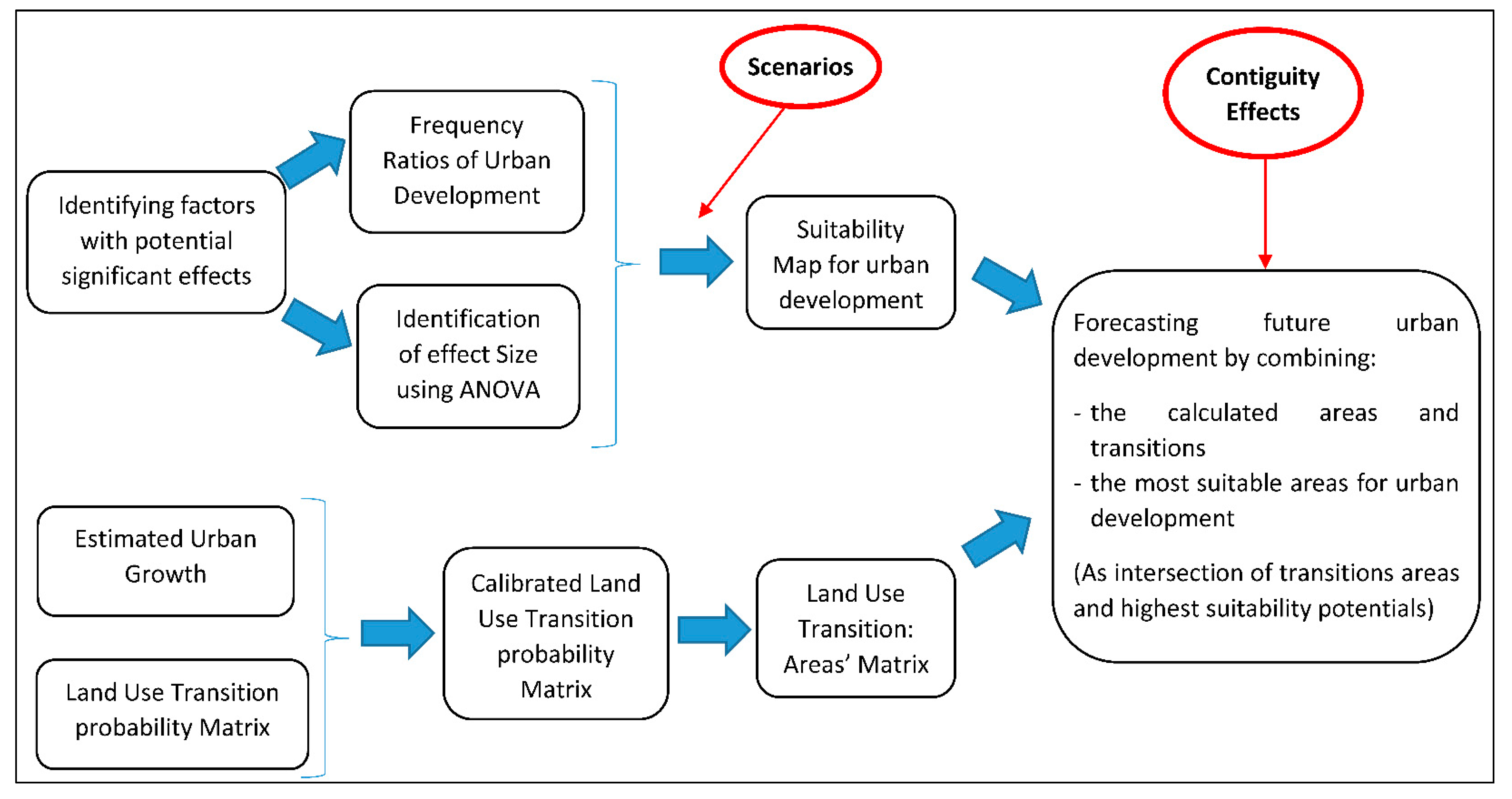
1.2. Framework of the Study

Understanding the effects, as types and sizes, of the driving factors of land use change represents an essential part in the case of examining scenarios. These scenarios could be defined with respect to anticipated events or policies, and also with respect to the evolution of socio-economic and environmental conditions. This research was conducted in the framework of a research project [41] studying the possible benefits of implementing solutions from the water–soil–energy nexus, i.e., the relationships between the usage and management of water, energy production and consumption, and the soils, both from the technical side and from the managerial one. Thus, the considered scenarios must be sensitive to the significant changes in factors steering the land use dynamics. Hence, the scenario-based simulations for urban dynamics necessitate understanding these interactions because the changes in these factors would define the anticipated scenarios.

Apropos of the proposed scenarios, three hypotheses were incorporated in this study: (1) the anticipation of global changes as an increase in oil prices and a wealth reduction; (2) local spatial changes as the provision of new rail lines and the development of new urban zone; and (3) assuming that new urban development will take place in proximity to existing urban development (contiguity effect). The objective of this study is to develop a methodology for the prediction of future urban dynamics, which could integrate driving factors, as well as several anticipated scenarios, in a flexible and understandable manner. The key requirements are the ability to define flexible scenarios and to examine the variations resulting from the changes of specifications of these scenarios. This need is clearly depicted during the phase of assessing the efficiency of socio-economic/infrastructural/environmental strategies and their impacts on land use. The developed approach in this study aims mainly to support the decision makers in the form of a guiding tool that deals, and in a separate form, with: (i) the dynamic evolution/interaction between land use classes, (ii) the spatial urban attractivity, and (iii) the mechanisms originating from spatial economics, along with additional data on urban dynamics.

The study area covers the denser area of the Île-de-France region. It was selected as the study area since it has witnessed significant internal and international migration movements’ destination as it represents a major center for high-ranking educational institutions and economic and employment opportunities, and because it provides better accessibility to opportunities, urban infrastructure, and services [42]. The results of the simulations under different scenarios are employed to assess the impacts of global prices and incomes changes in addition to local infrastructural changes on the spatial accessibility and the quality of the environment. The paper is organized as follows: the second section presents the developed methodology and the materials used as data collection and techniques. The third section highlights the obtained results which are discussed in more details in section four. Section five summarizes the paper as novelty and methodology and proposes some future research subjects related, as extension, to this research.

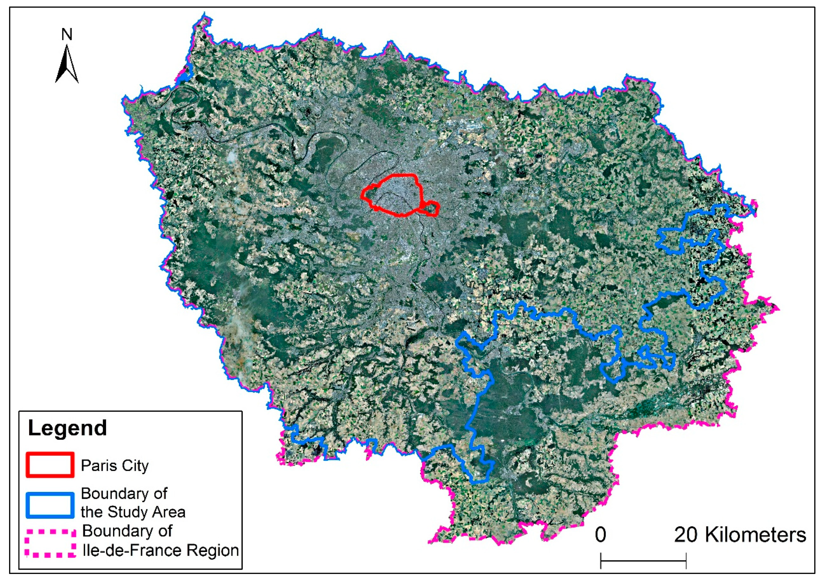
2. Materials and Methods

The study area covers a large surface of 9261 km² of the Île-de-France region. As the prospective work presented in this paper is the preliminary step of assessing several water–soil–energy solutions, such as the development of green roofs and facades, fatal heat recovery, or local management of rainwaters, the study area covers a large part of the Île-de-France region, for which open data are mostly available. The southeast part of the region for which data is not available is outside the main agglomeration of Paris. The study area is large enough to be considered a partly autonomous system for which variables can be isolated. In more detail, the study area is used to evaluate and perceive the effects of possible scenario changes at the global and local levels on the future land use dynamics. The predictions will be made for the year 2050. Figure 1 presents the study area. The city of Paris as well as the first ring appears to be quite dense, while there are many agricultural and green areas in the remaining of the territory.

The developed methodology (illustrated in Figure 2) has to generate projected land use maps under different scenarios as the final objective. These steps to reach this objective could be divided into two parts: (i) the formalized approach to introduce scenarios, and (ii) combining the spatial and quantitative projections. The key concepts of the methodology are represented by (a) the suitability maps that rank, spatially, the attractivity for urban development, (b) the amount of future urban development as well as the transition matrices between land classes, and lastly (c) the external factors that impact the spatial distribution of urban development. In this framework, the spatial part was presented by generating suitability maps for the potential future urban development. In the same context, the quantitative form is depicted by the interactive changes of areas between land use classes which are commonly known as the land use transition matrices.

Starting with the first process of producing suitability maps, several driving factors were identified for significant effects of urban development by using correlation analysis. The frequency ratios of urban development within the classes (natural break classes) of the identified significant factors were calculated to show the interactive distribution of urban areas relative to the changes in the values of these driving factors (as shown in Appendix A). These distributions are assumed to be the same for future projections. Additionally, and in order to integrate different socio-economic and spatial scenarios, the effect sizes on the urban development were calculated according to the statistical variance analysis of a multilinear regression model. On the other hand, the potential transitional interaction between land use classes was calculated based on estimating the growth of areas for these classes and then calibrating, by iterations, the mean matrix of the previous transition matrices. More details of these processes are indicated in the following subsections.

2.1. Spatial Form of Potential Urban Change (2018–2050): Generating Suitability Maps

This section presents the two processes used to generate the suitability map for future urban development until the horizon of the year 2050. The first process consists of identifying the significant factors that could affect the dynamics of urban evolution and presents how the corresponding data were collected. The second process presents a new methodological approach for introducing different scenarios of urban dynamics.

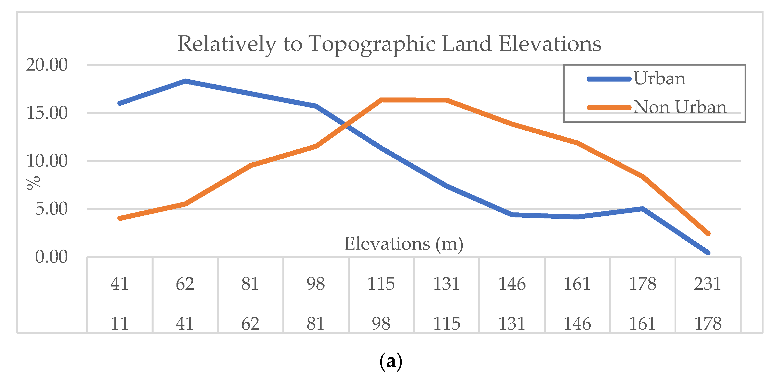
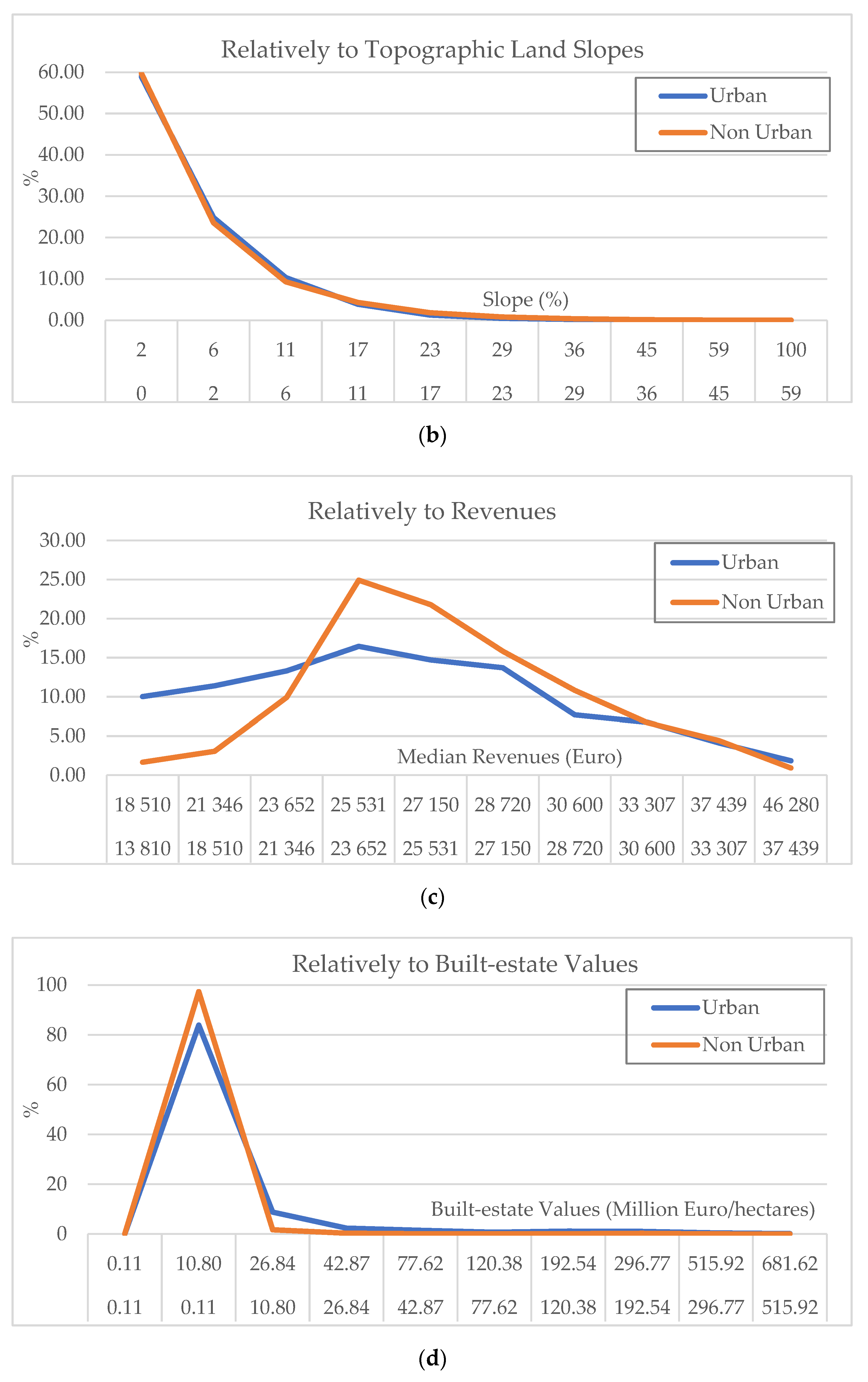
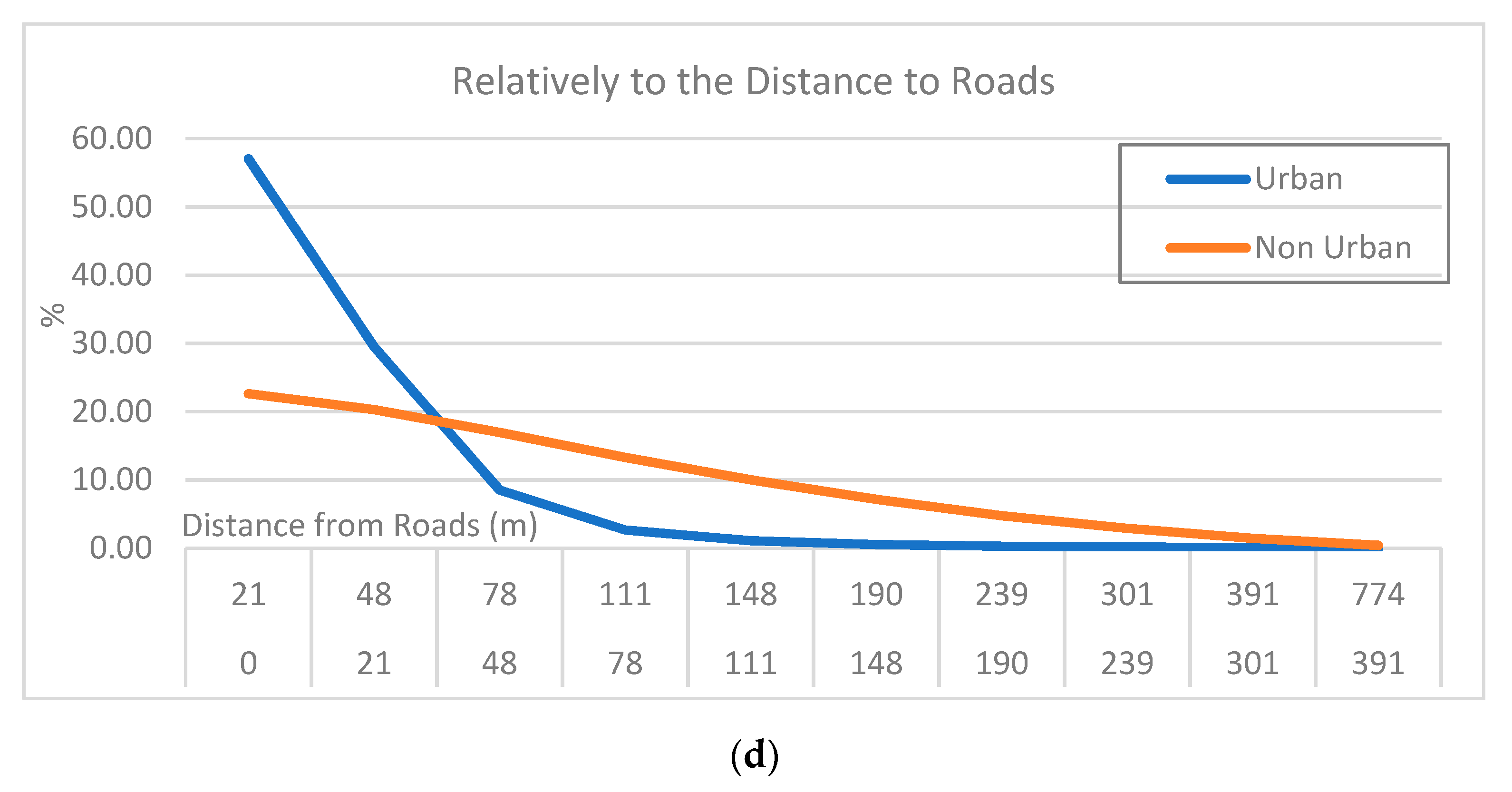
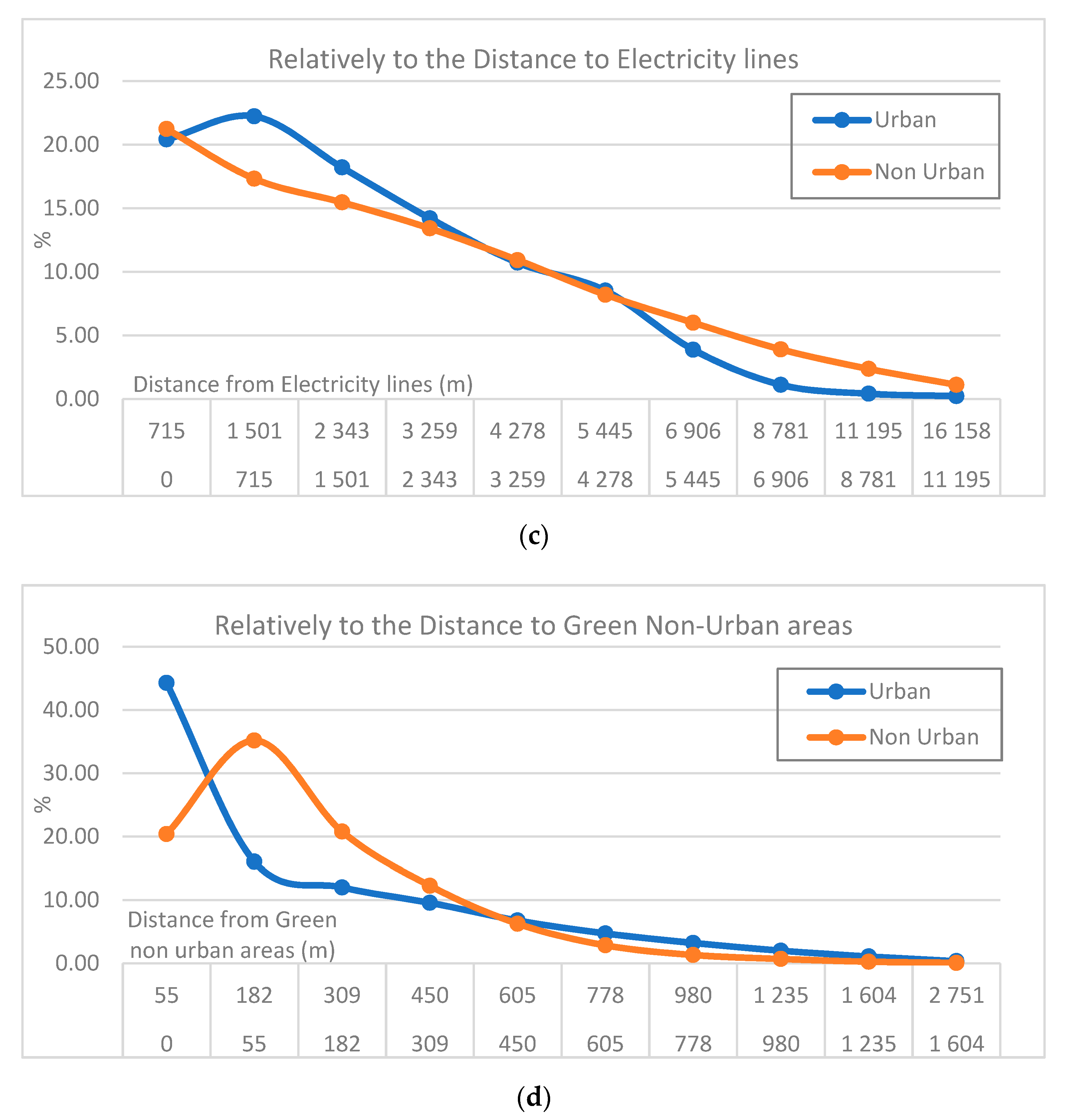
2.1.1. Identification of Factors with Significant Effects on Urban Development

Different variables that could affect the evolution of urban dynamics, were identified in previous literature studies [1,20] as geo-topographic, socioeconomic, infrastructural, and environmental factors. With the availability of data, some of these factors were selected for the study; however, additional factors were added. The selected factors were grouped similarly to previous studies.

The geo-topographic factors encompass land elevations and the slopes:

• The terrain characteristics were computed with the help of the digital elevation model (DEM) from the BDAlti database by IGN (2021) [43] by using the ArcMap 10.8 software.

The socioeconomic class includes population density, employment density, built-estate values, and revenues/income levels:

• The population and employment densities for the year 2017 were collected from the database of the population of the INSEE (2021) website [44].
• The average built estate values over the period 2016–2020 were calculated based on the data obtained from the website cadredeville (2021) [45]. It should be noted here that the non-available data of built estate values for the “Charmont” locality were interpolated, based on the available data, by applying the inverse distance weighting method in ArcMap 10.8.
• The income levels for the year 2018 were obtained from the website INSEE-FILOSOFI (2021) [46].

The infrastructural class includes the Euclidean distances from roads, highways, rails network, and high-voltage electricity lines:

• The vector data of road, highways, and rail networks, as well as the water streams and rivers, and high-voltage lines were collected from OpenStreetMap [47].

The environmental class includes the distance from water streams and from green non-urban areas including agriculture areas, forests, and wetlands:

• These indicators were computed from the land use data provided by UrbanAtlas (2021) [48].

The primary data collected and used for the land use dynamics were the land use classification maps generated and provided by UrbanAtlas (2021) [48].

The available three land use maps for the years 2006, 2012, and 2018 were rasterized to raster datasets of 25-m pixel resolution, after unifying the land use class into six general classes: (1) urban built-up areas, (2) green urban areas including public gardens, parks, etc., (3) green non-urban areas which encompass cultivation zones, forests and wetlands, (4) areas dedicated for land transport systems like roads, highways and rails network, (5) bare soil lands, and (6) water streams, rivers, and lakes. The pixel resolution of 25-m was selected in order to unify the pixel size for all the rasterized datasets since it represents the minimum resolution among the available data and corresponds to that of the DEM. The rasterized datasets are published and publicly available in the Mendeley Data repository: https://data.mendeley.com/datasets/2mvpr7vdb3/2.

Figure 3 shows the maps’ presentation of these data. Some data are network-based, and thus the structure of the maps is clearly polarized by either the roads, the train lines, the electricity network, or the streams. Others show gradients from center to periphery.

The incomes exhibit a different configuration, with higher prices in the west of the region. In order to identify the significant driving factors for the urban development in the study area, a correlation analysis of the evolution of urban areas with respect to each factor was conducted. Therefore, different maps for these factors were produced and then clustered by dividing these data into 10 classes by using the Jenks’ Break classification in ArcMap 10.8 software. The share ratios of the urban (built-up) area in each of these classes, relative to the total urban areas, were compared to those of non-urban areas. Appendix B, Figure A1, Figure A2 and Figure A3 show approximately some perfect correlations for land slopes and distance from water streams; consequently, these factors were not taken into account. The aforementioned comparative analysis shows the possible significant factors; nonetheless, additional analysis is required to assess the effect sizes of these variables. Accordingly, the variance statistical analysis (ANOVA) for a multilinear regression model of the primary significant factors, was conducted in R software using 1,477,075 observations after aggregating the pixels in patches of 10 by10. The results obtained from this test show (

Table 1. Effects sizes of driving factors.

Factor	Sum Square	% Initial Effects Sizes (%) (Based on ANOVA Test)
Distance to Green non-urban areas	140,094	0
Population Density	40,334,070	53
Employment Density	4,790,721	6
Median Revenues	214,723	0
Distance to high voltage Electricity Lines	1,805,170	3
Distance to Highways	4,054,164	6
Distance to Rail lines	4,063,927	6
Distance to Roads	14,966,116	20
Built-estate Values	1,919,125	3
Elevations	2,269,003	3

): (i) major effect sizes of population density and distance to roads with 53% and 20%, respectively; (ii) a size-effect of 6% for the employment density and distance to highways as well as for the distance to rail lines; (iii) an effect size of 3% for land elevations, built-estate values and likewise for the distance to high-voltage electricity lines; and (iv) very negligible effects for the income levels and for the distance to green non-urban areas. In consequence, the latter factors were not taken into account in generating the suitability maps for urban development.

The suitability maps were generated in ArcMap 10.8 software by summing the weighted normalized frequency ratio rasters. In more details, the Jenks’ classes for each of the final selected driving factors were converted by reclassification module to the corresponding frequency ratios of urban development.

This process leads to the production of frequency ratio rasters for the driving factors. After normalization, the final rasters were weighted according to the ANOVA size effects prior to the sum of all pixel values. The summation map was also normalized and converted to percentages. Suitability maps are presented and analyzed in the Results section (Figure 4). They show the urban suitability map as percentages of potential urban attractivity.

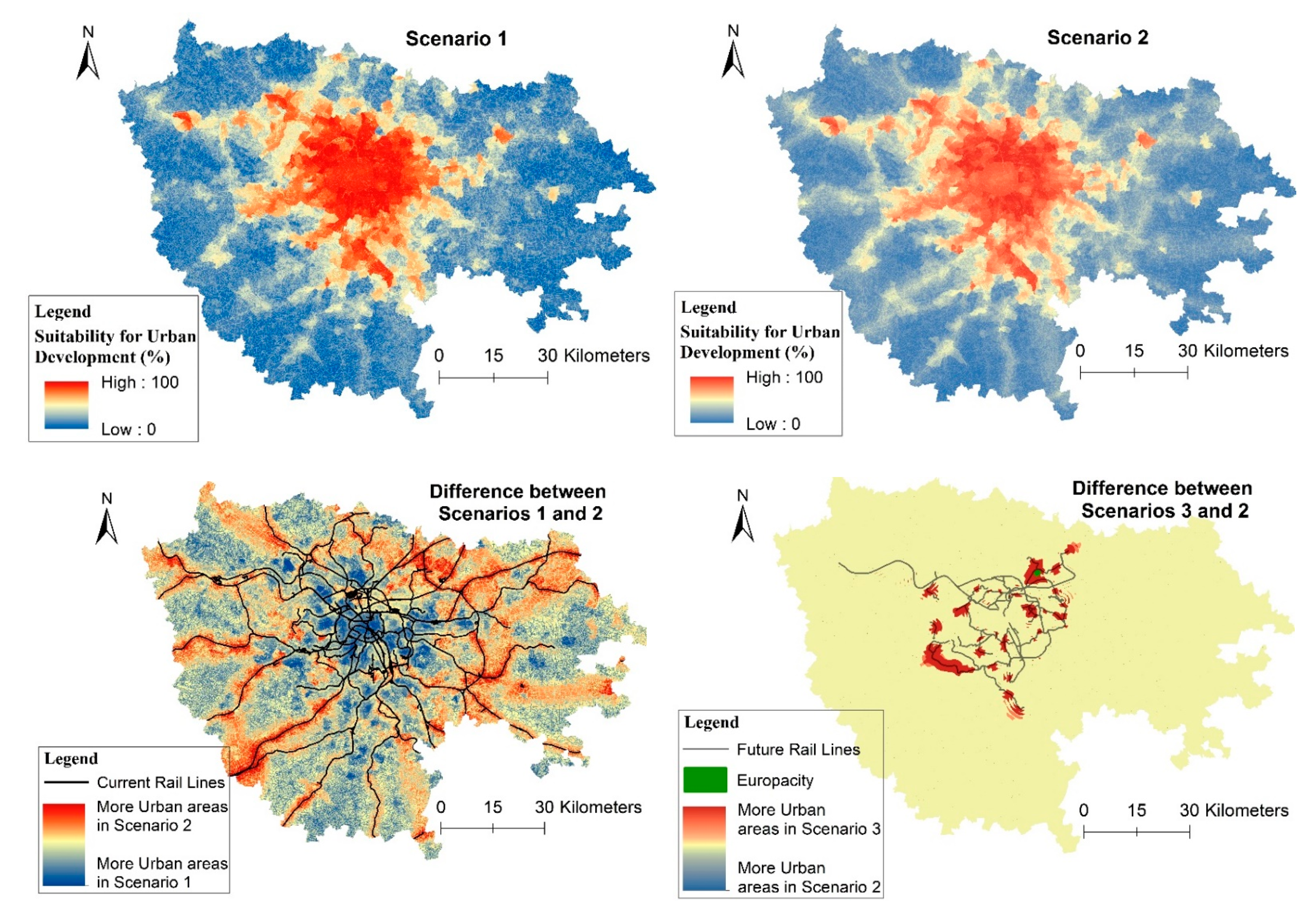
2.1.2. Scenarios for Urban Suitability

Three scenarios for future land use development, mainly the urban development, are considered for the process of projecting the evolution.

The first scenario, which was presented previously in sub-Section 2.1.1, is the “business as usual” one.

It is parameterized by (i) the frequency ratios of urban development in different classes of the significant driving factors and (ii) the size effects of these factors obtained from the aforementioned variance analysis.

The second scenario simulates the effect of global changes. It takes into account an elevation in the oil price, which is assumed to be concomitant to a decrease in global wealth. In this context, the effect sizes for employment density, income levels, distance to highways, and distance to rail lines are likely to increase and will be updated accordingly in the parametrization.

Thus, the future urban development will likely be more concentrated around economic activity zones that have higher accessibility, and also more concentrated around public transport services, such as buses in highways and rail transport modes.

The objective of this procedure is not at the moment to quantify the exact rate of changes in an ultimate manner, but rather to develop a method to introduce the scenarios.

Within the framework of this, 25% of the total effects will be assumed to be distributed additionally for the increasing factors; consequently, in total the increasing factors, having 18% effect value in scenario 1, will have a size effect of 43% for the scenario 2.

It is assumed specifically that revenues will have a 6% for scenario 2 instead of 0 (for scenario 1). The remaining additional percentage will be distributed proportionally to other factors.

Table 2. Effects sizes for scenarios 1 and 2.

Factor	% Initial Effects Sizes (%) (Based on ANOVA Test)	Modified Effects Sizes (%) for Scenario 2
Population Density	53	37
Employment Density	6	13
Median Revenues	0	6
Distance to high voltage Electricity Lines	3	2
Distance to Highways	6	12
Distance to Rail lines	6	12
Distance to Roads	20	14
Built-estate Values	3	2
Elevations	3	2

shows a comparison of initial (scenario 1) and modified effects size (scenario 2).

The process of producing the suitability maps for scenario 2 is similar to that of scenario 1 but by using the modified effect values.

Additionally, the third scenario differs from the second one by considering some changes at the local level, specifically the changes in the infrastructure and the planned future urban areas.

In this scenario, the expansion of the Rails network after the year 2018 [49] and the development of the EuropaCity project [50] were taken into consideration. The development of the Grand Paris Express network is planned, but not fully financed yet.

This scenario supposes that the entire network is implemented. EuropaCity is a large activity district that might bring new economic opportunities, but whose ecological impacts are questioned. It is supposed to be implemented as initially planned. Thus, scenario 3 differs from scenario 2 by two kinds of local interventions: a new network, and a new activity zone.

These scenarios are introduced in the prediction processes for generating new suitability maps.

2.2. Quantitative Urban Change (2018–2050)

2.2.1. Urban Growth

The rates of urban growth for the periods 2006–2012 and 2012–2018 were used and compared to estimate, by projections, the possible urban growth rate between the years 2018 and 2050.

By examining the urban growth rates for the periods 2006–2012 and 2012–2018, an increase/acceleration in urban growth rate by 0.06% was observed between these two periods.

Based on this, an assumption of a possible increase by 0.06% every 6 years was considered. Similarly, a possible decrease of 0.013% and 0.012% every 6 years was considered by assumption for bare soil and green non-urban areas, respectively. In a different way, the actual annual growth rates of 0.025% and 0.14% for the period 2006–2018 were considered for green urban areas and lands of road and rail transport infrastructure.

These latter two values were selected because the annual rate of growth for (i) the green urban areas show positive and negative values for the periods 2006–2012 and 2012–2018, and (ii) lands dedicated for roads and rail would lead to a projected growth rate value of 0% for the period 2024–2030 in case of using the same deceleration rate for 6 years period.

Based on these growth values, the projections for the year 2050 show (i) an increase in the urban areas and the green urban areas as well as the areas of roads and rail lands by 18%, 1%, and 5% respectively; and (ii) a decrease in the areas of green non-urban and bare soil lands by 4% and 25%, respectively, compared to the year 2018.

The water zones, as streams and rivers, were considered not altered (neither increase nor decrease). These estimations are not the main subject of this study’s problem, which is defined as the possibility of developing a new methodology for introducing factors-based scenarios of land use projections.

These estimated values will be used for a matching distribution over the potential transition matrix for the period extending between the years 2018 and 2050 as indicated in the following section.

2.2.2. Land Use Transitions

The land use transition matrices for the periods 2006–2012, 2012–2018, and 2006–2018 were obtained from the land use maps [48] by using the Molusce extension of QGIS 2.18 software. An average matrix consisting of average values for the aforementioned matrices was calculated to represent the actual land use transition matrix over these periods.

This matrix was used, in addition to the growth rates of all land use classes as aforementioned in the previous section, to estimate the future 2018–2050 transition matrix.

The estimation of the new matrix was based on calibrating, by many iterations, the values for the actual matrix to reach matching compatibility with the future increase/decrease rasters for all land use classes.

Table 3. Actual LU transition matrix.

	Urban Areas	Urban Green Areas	Agriculture, Forests and Wetlands	Roads and Rails Dedicated Areas	Bare Soil	Water
Urban Areas	0.9923	0.001	0.0053	0.0006	0.0007	0.0001
Urban Green Areas	0.0121	0.9874	0	0.0002	0.0003	0
Agriculture, Forests and Wetlands	0.0078	0.0001	0.9915	0.0003	0.0002	0.0001
Roads and Rails dedicated areas	0.0037	0.0001	0.0002	0.9959	0.0001	0
Bare Soil	0.2854	0.016	0.0026	0.0048	0.6912	0
Water	0.0028	0	0	0	0	0.9972

and

Table 4. Calibrated LU transition matrix.

	Urban Areas	Urban Green Areas	Agriculture, Forests and Wetlands	Roads and Rails Dedicated Areas	Bare Soil	Water
Urban Areas	0.9921	0.0016	0.0041	0.0021	0.0001	0
Urban Green Areas	0.0121	0.9874	0	0.0002	0.0003	0
Agriculture, Forests and Wetlands	0.0597	0.0001	0.9397	0.0004	0.0001	0
Roads and Rails dedicated areas	0.0037	0.0001	0.0002	0.9959	0.0001	0
Bare Soil	0.2854	0.0160	0.0026	0.0048	0.6912	0
Water	0	0	0	0	0	1

depict the actual and estimated matrices.

2.3. Spatial Distribution of Urban Changes

The projected land use maps are generated by allocating the new urban areas, according to the rate of urban changes, with respect to the spatial distribution of suitability maps. In other words, the number of pixels corresponding to the new urban areas will be allocated by converting land use classes, different than urban areas, into urban areas by allocating the pixels with the highest suitability scores. Note that some of these pixels have the same suitability score, and within these limits, an additional contiguity criterion was added.

The suitability maps, depending on identified driving factors, reflect the global/international, and local trends in some of the driving factors as the changes in oil prices, the wealth, and the infrastructural services. The approach could also be extended to design more sophisticated scenarios, for instance with new technological advances or emerging employment patterns. The contiguity effect is assured by the effects’ sizes of the driving factors where the urban expansion could, for instance, take place in a gradient shape as distances from the locations of attracting activities/infrastructure.

Further elaborated, the contiguity effect was taken into consideration in the form of the shortest distance to urban areas. This concept of the shortest distance was divided into two parts: (i) the actual Euclidean distance to the nearest urban areas, and (ii) the location in a zone with more urban areas. The latter part could be depicted by the aggregation of pixels in order to make a comparison of pixels with similar suitability scores and the same distance to the nearest urban area. In this context, the aggregation starts with small to larger pixel sizes to allow further comparison.

3. Results and Discussion

3.1. Suitability Maps

Figure 4 shows the urban suitability maps as well as the difference among the proposed scenarios.

Visually, scenario 3 is very similar to scenario 2 and hence its suitability map was omitted. However, the difference between the suitability map of scenario 2 and scenario 3 is included. The main difference between scenarios 2 and 1 is linked to the hypothesis of an increase in oil prices and a decrease in wealth. As expected, the potential urban development is more concentrated around the rail lines in scenario 2.

Moreover, the center of the agglomeration is becoming too expensive. The differences observed between the suitability maps of scenarios 3 and 2 are local. The EuropaCity area is indeed very attractive for new settlements.

However, the attractiveness of the new transit lines differs spatially, according to the nature of the existing neighborhoods. The existing transit lines have a much more attractive effect on urban developments than the new ones in this simulation.

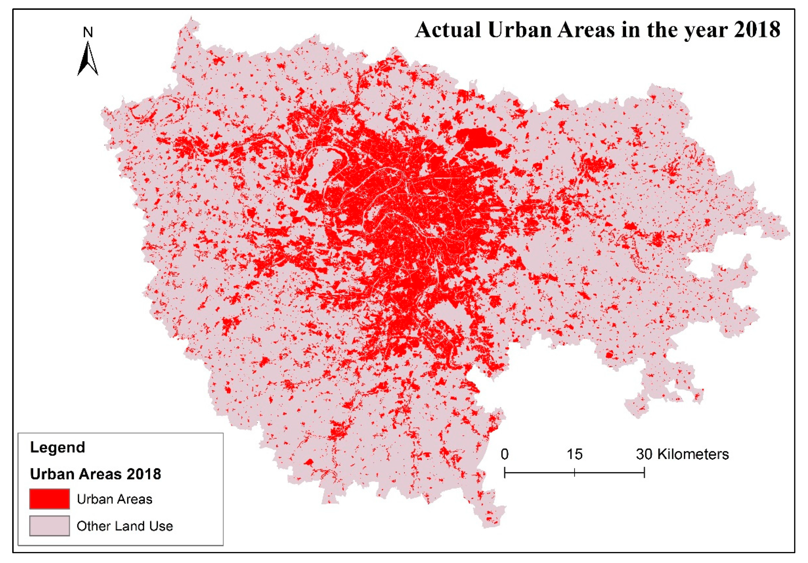
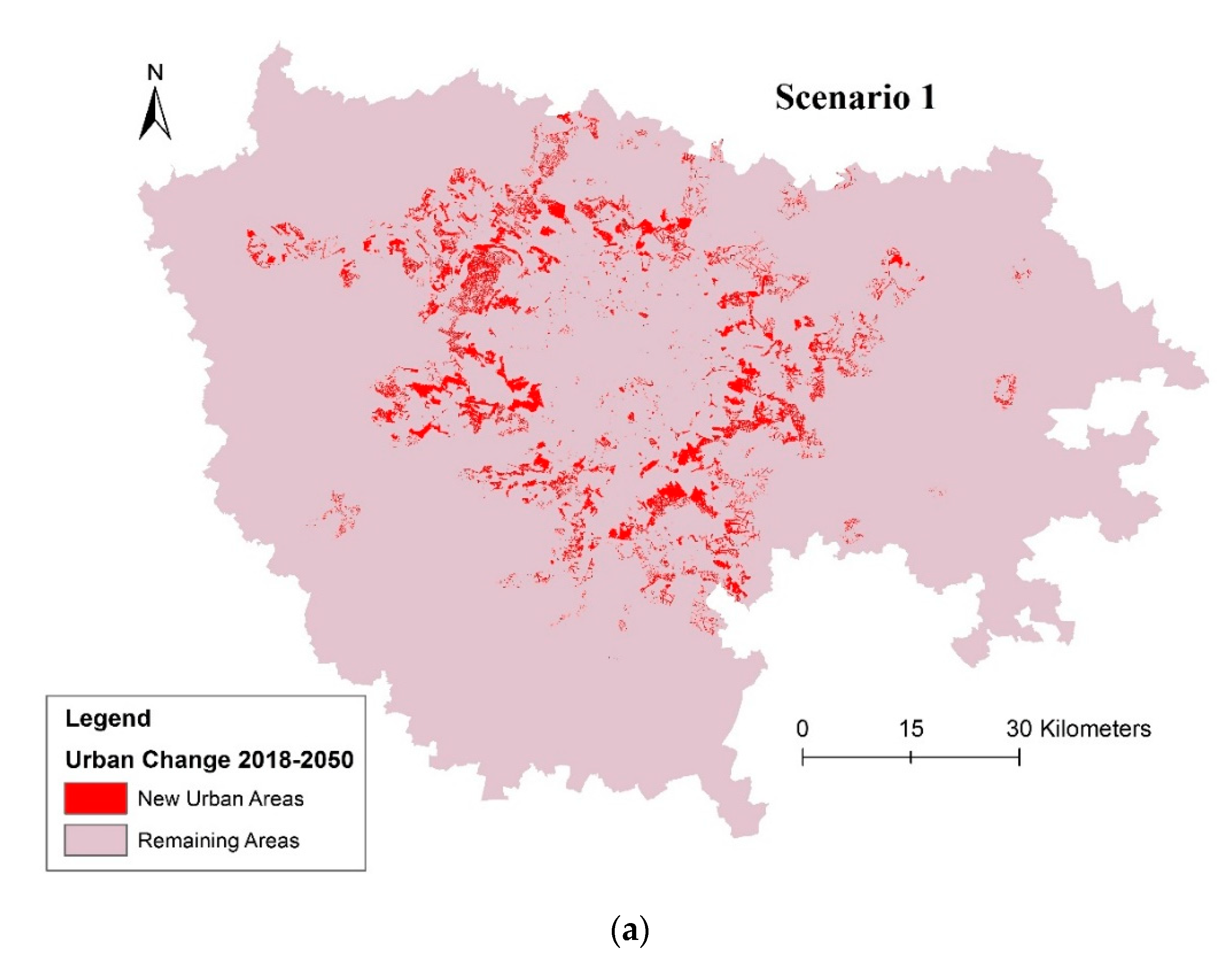
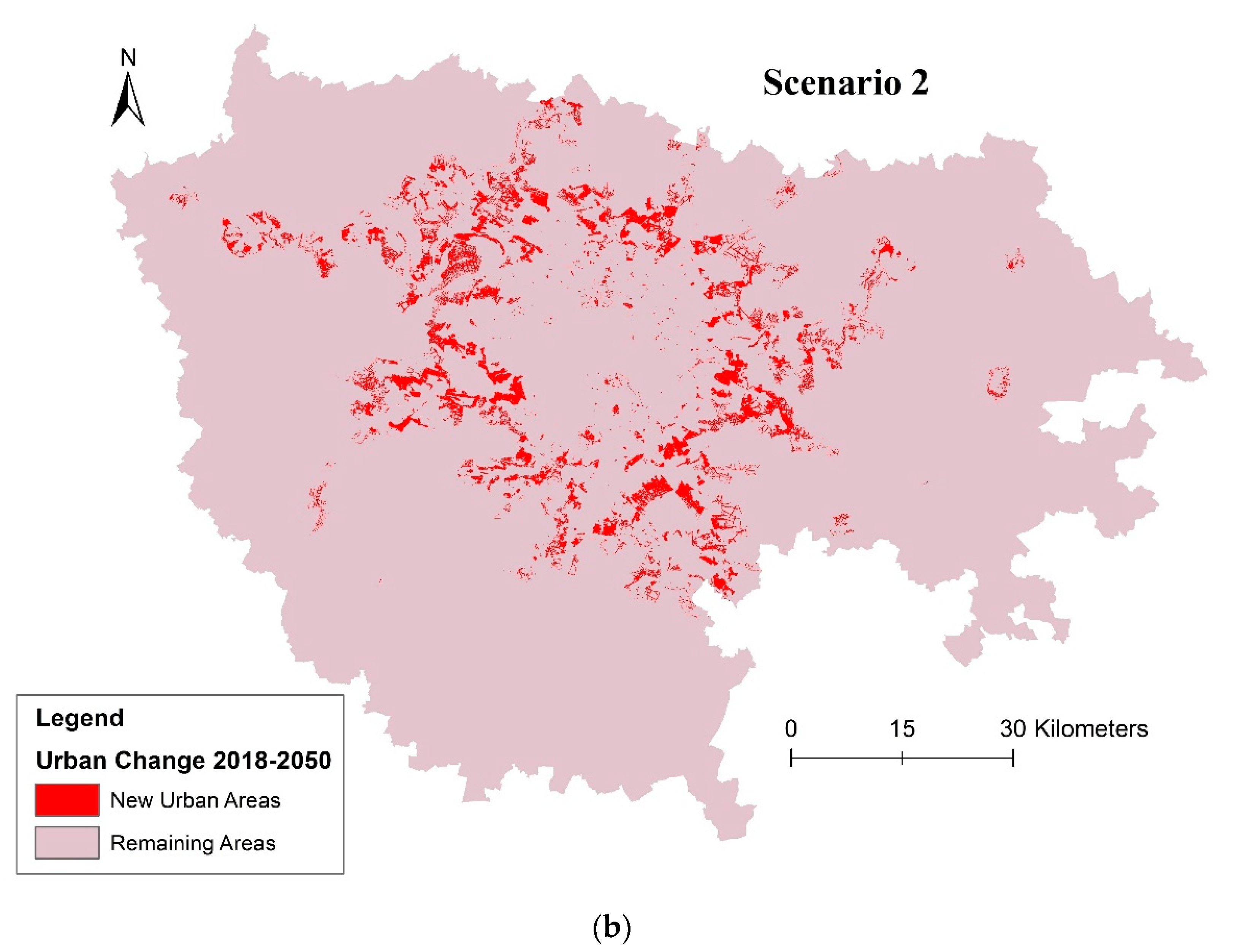
3.2. Projection of Urban Development

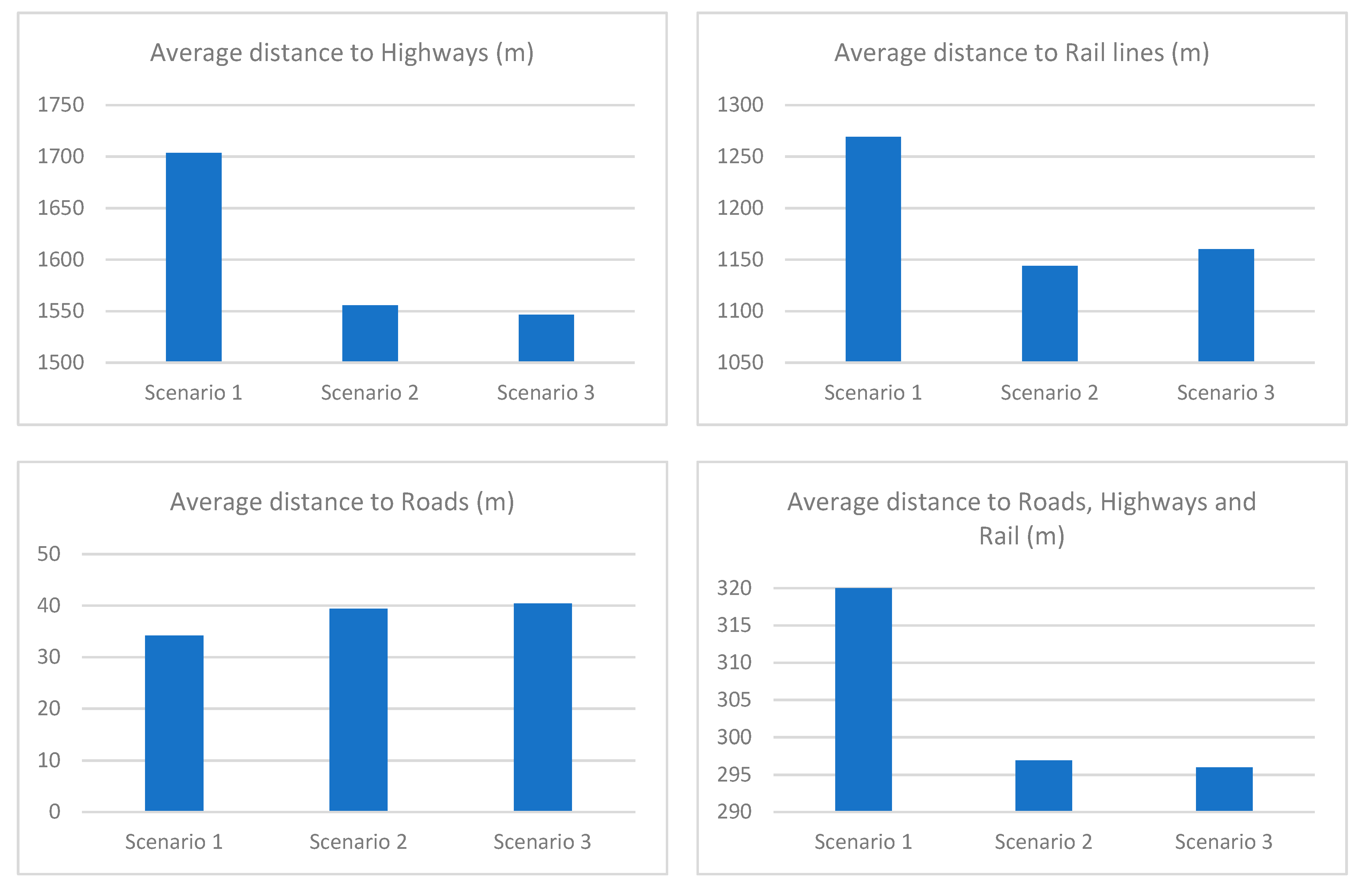
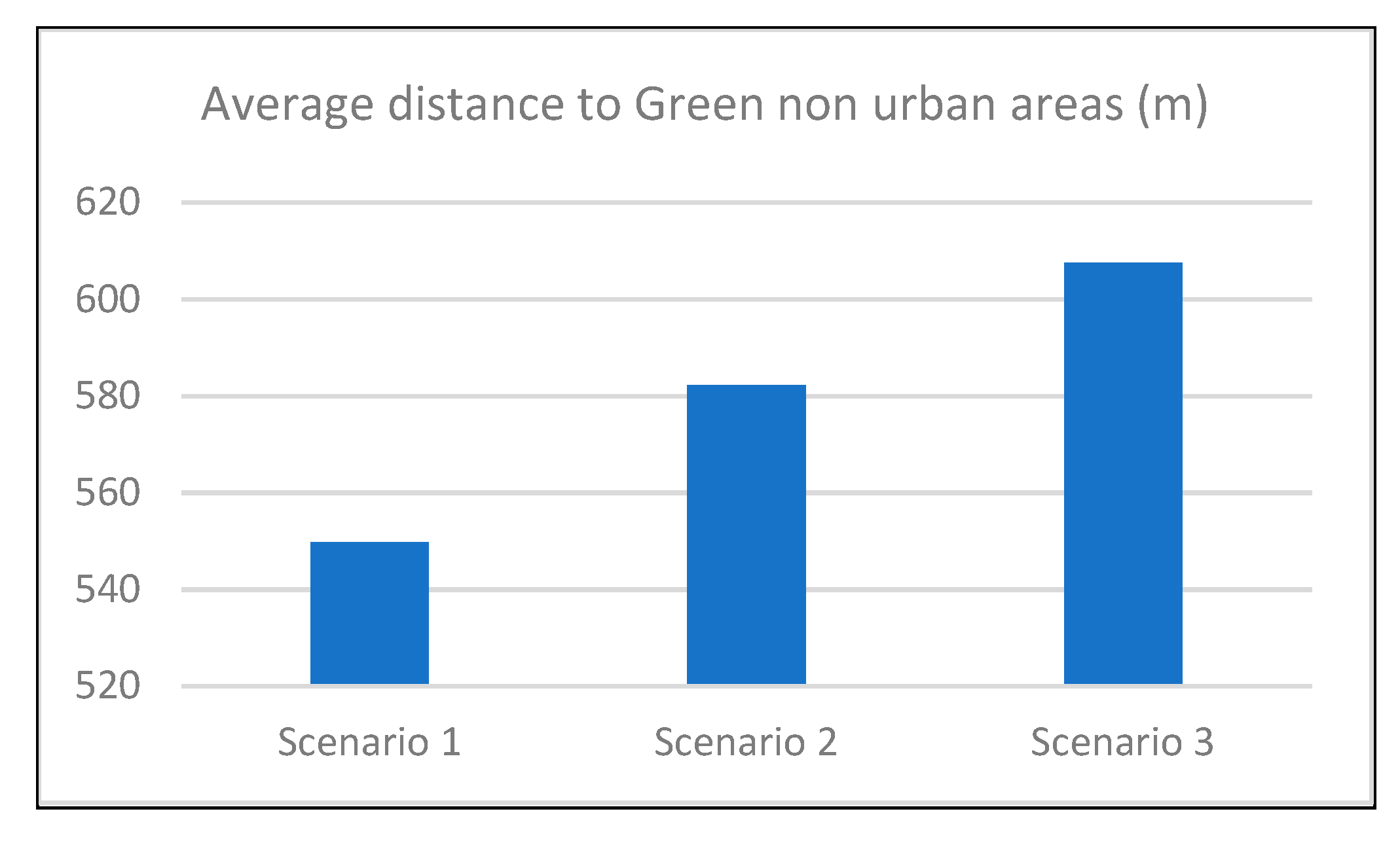
Figure 5 and Figure 6 show the actual and the projected land use maps, under scenarios 1 and 2, for the years 2018 and 2050, respectively.

Figure 6b is quite similar to Figure 6a; however, the development zones are a bit more concentrated around the transit lines.

3.3. Analysis

The simulated urban change maps, for the three scenarios, between the years 2018 and 2050 show different characteristics of geographic and spatial distribution. These different characteristics will induce dissimilar interactions with other land use classes, infrastructures and services.

More closely, the accessibility to transport services and to green non-urban areas such as forests, cultivation lands, and wetlands will only be discussed in this study.

In terms of distance, the accessibility of new urban areas, to be developed between the years 2018 and 2050, were compared among the three proposed scenarios. Figure 7 shows greater accessibility for scenarios 2 and 3, depicted as short distances, to highways and rail lines characterized by more public transportation than other roads. In contrast, the average accessibility to roads for urban areas in scenario 1 is more than the ones of other scenarios.

Generally, the accessibility to all transport modes (private vehicles, rail and road public transport modes) for scenarios 2 and 3 is greater than that of scenario 1.

In addition, the proximity to green non-urban areas, such as forests/agricultural land/wetlands, is lower for scenarios 2 and 3 relative to that of scenario 1, as indicated in Figure 8, because the urban areas are potentially supposed to take place in the surroundings of and in areas well served by public transport systems with low accessibility to green non-urban areas.

The obtained results are, reasonably, in conformity with the selected and modified criteria when setting up the scenarios.

These calculated characteristics could give indications for planners and decision makers on the possible tendencies of future urban development under different conditions.

These tendencies are explained in terms of spatial distributions and their corresponding demands for service infrastructures and updates/new urban master plans. Based on these methodic approaches of predictions and by inserting the scenarios, the decision makers, planners, and urban developers would anticipate changes of their subjects of interest, plan and steer future urban development accordingly, and mitigate the perceived risks.

The decentralization as the development of new urban centers and the redevelopment shapes as steering the previous urban development toward vertical expansion was not investigated in this study; however, this information, when available, could give more indicative information and allows to update, more precisely, the used methodology. More precisely, the contiguity to old urban areas was taken into consideration in this study; however, this could represent a limitation since this concept did not take into consideration the development of new urban areas as new centers and not as an expansion of old zones.

Also, the integration of urban masterplans and their regulations, such as restricted/reserved areas, the maximum allowable heights of buildings and buildings capacity, in addition to the anticipated urban and economic projects could be studied further in the context of future research directions.

Moreover, a comparative analysis of the methodological approaches of the used methodology in this research and the Cellular Automata models need to be assessed. The authors consider the CA, coupled with Markov Chain transitions, a good model to replicate the previous urban development based on contiguity effects. However, the limitations could be perceived as the limits of the predefined urban contiguity matrix which could not necessarily, for the majority of cases, predict the future urban development. In that context, the authors propose the development of a more sophisticated model consisting of a 3D adaptive matrix that could be used to predict future development and the interactions with other land covers/land use classes. The adaptiveness of this matrix should be represented by the continuous calibration according to the spatial context, socio-economic environment, the infrastructural services, policies, and strategies and the new shapes of urban development.

Indeed, the proposed contiguity criterion differs from that of the CA models, which is based on spatial changes according to a predefined contiguity matrix. Relying on a predefined contiguity matrix could not always represent the reality of urban expansion which in most cases does not follow a spatial shape/matrix. In other words, the CA-MCM models were not used here to simulate the future land use distribution since these models rely only on replicating the previous trend/s of land use evolution within a spatial contiguity framework.

One of the already mentioned limitations of CA-MCM models is the difficulty to incorporate external factors. Different socio-economic factors, geo-topographic aspects in addition to the existence of infrastructure could determine the evolution of population growth in addition to locations of future urban development and also the conversions/interactions between different land use classes.

ML models do have the possibility to take into account external factors. However, the lack of interpretability of the models impairs the possibility to discuss any step of the models with local decision makers, as well as with researchers from other disciplines, notably hydrology and environmental sciences.

4. Conclusions

Predicting the evolution of land cover is generally a difficult task, because of the sparsity of historical data and the lack of clear causal effects between factors and land use dynamics.

Many statistical approaches focus on minimizing, in terms of error, the difference between the predicted evolutions and the actual ones. This possible drawback of these approaches is that they cannot easily incorporate external factors, and tend to predict, more or less, always the same dynamics.

On the other hand, the economic approaches are purely based on mechanisms. However, they only represent stylized facts and cannot easily be used to investigate the evolution of actual territories. Spatial econometrics approaches are, indeed, data-based models but tend to be rather complex and require much data.

Lastly, the classical geographical spatial models such as CA or CAMCM cannot always integrate the urban development driving factors.

Thus, developing a methodology that could integrate the driving factors for urban development, as well as the corresponding scenarios, in a flexible and understandable manner is exacted. The comprehension and the flexibility of introducing scenarios is an essential part of the process of predicting land use distributions since the need to examine the variations accompanied as a result of changing specific and defined parameters is important, especially when linking the strategies for land use with other socio-economic/infrastructural/environmental plans.

As the approach developed in this paper is mainly targeted at supporting decision-making, it is presented as simply as possible and tries to separate clearly between the spatial urban attractivity and the dynamic evolution/interaction between land use classes. In addition, it is enriched with mechanisms originating from spatial economics, along with more detailed data on urban dynamics.

Certainly, simulating further the global strategies of residents, property developers and local policy-makers would enable to add a feedback loop in the dynamics of land use evolution. Moreover, special attention must be paid to the heterogeneity of the spatial dynamics: privileged directions for growth, expansion rates, etc. This will be the objective of future research.

References

1. Kim, Y.; Newman, G.; Güneralp, B. A review of driving factors, scenarios, and topics in urban land change models. Land 2020, 9, 246. [Google Scholar] [CrossRef]
2. Aburas, M.M.; Ahamad, M.S.S.; Omar, N.Q. Spatio-temporal simulation and prediction of land-use change using conventional and machine learning models: A review. Environ. Monit. Assess. 2019, 191, 205. [Google Scholar] [CrossRef] [PubMed]
3. Rosenzweig, C.; Solecki, W.; Romero-Lankao, P.; Mehrotra, S.; Dhakal, S.; Bowman, T.; Ali Ibrahim, S. ARC3.2 Summary for City Leaders—Climate Change and Cities: Second Assessment Report of the Urban Climate Change Research Network; Columbia University: New York, NY, USA, 2015. [Google Scholar]
4. Oke, T.R. Boundary Layer Climates, 2nd ed.; Taylor and Francis: Abingdon, UK, 1987. [Google Scholar]
5. Han, Y.; Jia, H. Simulating the spatial dynamics of urban growth with an integrated modeling approach: A case study of Foshan, China. Ecol. Model. 2016, 353, 107–116. [Google Scholar] [CrossRef]
6. Clark, D. Urban Geography: An Introductory Guide; Taylor & Francis: Didcot, UK, 1982. [Google Scholar]
7. Liu, M.; Hu, Y.; Chang, Y.; He, X.; Zhang, W. Land use and land cover change analysis and prediction in the upper reaches of the Minjiang River, China. Environ. Manag. 2009, 43, 899–907. [Google Scholar] [CrossRef] [PubMed]
8. Han, H.; Yang, C.; Song, J. Scenario simulation and the prediction of land use and land cover change in Beijing, China. Sustainability 2015, 7, 4260–4279. [Google Scholar] [CrossRef] [Green Version]
9. Chang, X.; Zhang, F.; Cong, K.; Liu, X. Scenario simulation of land use and land cover change in mining area. Sci. Rep. 2021, 11, 12910. [Google Scholar] [CrossRef]
10. Al-Shaar, W.; Nehme, N.; Gérard, J.A. The applicability of the extended markov chain model to the land use dynamics in Lebanon. Arab. J. Sci. Eng. 2020, 46, 495–508. [Google Scholar] [CrossRef]
11. Al-Shaar, W.; Gérard, J.A.; Nehme, N.; Lakiss, H.; Barakat, L.B. Application of modified cellular automata Markov chain model: Forecasting land use pattern in Lebanon. Model. Earth Syst. Environ. 2021, 7, 1321–1335. [Google Scholar] [CrossRef]
12. Al-Sharif, A.A.A.; Pradhan, B. Monitoring and predicting land use change in Tripoli Metropolitan City using an integrated Markov chain and cellular automata models in GIS. Arab. J. Geosci. 2014, 7, 4291–4301. [Google Scholar] [CrossRef]
13. KantaKumar, N.L.; Sawant, N.G.; Kumar, S. Forecasting urban growth based on GIS, RS and SLEUTH model in Pune metropolitan area. Int. J. Geomat. Geosci. 2011, 2, 568–579. [Google Scholar]
14. Araya, Y.H.; Cabral, P. Analysis and modeling of urban land cover change in Setúbal and Sesimbra, Portugal. Remote Sens. 2010, 2, 1549–1563. [Google Scholar] [CrossRef] [Green Version]
15. Mustafa, A.; Rienow, A.; Saadi, I.; Cools, M.; Teller, J. Comparing support vector machines with logistic regression for calibrating cellular automata land use change models. Eur. J. Remote Sens. 2018, 51, 391–401. [Google Scholar] [CrossRef]
16. Stamellou, E.; Kalogeropoulos, K.; Stathopoulos, N.; Tsesmelis, D.E.; Louka, P.; Apostolidis, V.; Tsatsaris, A. A GIS-cellular automata-based model for coupling urban sprawl and flood susceptibility assessment. Hydrology 2021, 8, 159. [Google Scholar] [CrossRef]
17. Saxena, A.; Jat, M.K. Land suitability and urban growth modeling: Development of SLEUTH-Suitability. Comput. Environ. Urban. Syst. 2020, 81, 101475. [Google Scholar] [CrossRef]
18. Martellozzo, F.; Amato, F.; Murgante, B.; Clarke, K.C. Modelling the impact of urban growth on agriculture and natural land in Italy to 2030. Appl. Geogr. 2018, 91, 156–167. [Google Scholar] [CrossRef] [Green Version]
19. Mahiny, A.S.; Clarke, K. Guiding SLEUTH land-use/land-cover change modeling using multicriteria evaluation: Towards dynamic sustainable land-use planning. Environ. Plan. B Plan. Des. 2012, 39, 925–944. [Google Scholar] [CrossRef]
20. Aburas, M.M.; Ho, Y.M.; Ramli, M.F.; Ash’Aari, Z.H. Improving the capability of an integrated CA-Markov model to simulate spatio-temporal urban growth trends using an Analytical Hierarchy Process and Frequency Ratio. Int. J. Appl. Earth Obs. Geoinf. 2017, 59, 65–78. [Google Scholar] [CrossRef]
21. Li, X.; Liu, X. Defining agents’ behaviors to simulate complex residential development using multicriteria evaluation. J. Environ. Manag. 2007, 85, 1063–1075. [Google Scholar] [CrossRef]
22. Arsanjani, J.J.; Helbich, M.; Vaz, E.D.N. Spatiotemporal simulation of urban growth patterns using agent-based modeling: The case of Tehran. Cities 2013, 32, 33–42. [Google Scholar] [CrossRef]
23. Samardžić-Petrović, M.; Kovačević, M.; Bajat, B.; Dragićević, S. Machine learning techniques for modelling short term land-use change. ISPRS Int. J. Geo-Inf. 2017, 6, 387. [Google Scholar] [CrossRef] [Green Version]
24. Abdullahi, S.; Pradhan, B.; Mojaddadi, H. City compactness: Assessing the influence of the growth of residential land use. J. Urban. Technol. 2018, 25, 21–46. [Google Scholar] [CrossRef]
25. Salman Aal-shamkhi, A.D.; Mojaddadi, H.; Pradhan, B.; Abdullahi, S. Extraction and modeling of urban sprawl development in Karbala City using VHR satellite imagery. In Spatial Modeling and Assessment of Urban Form: Analysis of Urban Growth: From Sprawl to Compact Using Geospatial Data; Pradhan, B., Ed.; Springer International Publishing: Cham, Switzerland, 2017; pp. 281–296. [Google Scholar]
26. Abdullahi, S.; Pradhan, B. Sustainable brownfields land use change modeling using GIS-based weights-of-evidence approach. Appl. Spat. Anal. Policy 2015, 9, 21–38. [Google Scholar] [CrossRef]
27. Park, S.; Jeon, S.; Choi, C. Mapping urban growth probability in South Korea: Comparison of frequency ratio, analytic hierarchy process, and logistic regression models and use of the environmental conservation value assessment. Landsc. Ecol. Eng. 2012, 8, 17–31. [Google Scholar] [CrossRef]
28. Kamaraj, M.; Rangarajan, S. Predicting the future land use and land cover changes for Bhavani basin, Tamil Nadu, India, using QGIS MOLUSCE plugin. Environ. Sci. Pollut. Res. 2022. [Google Scholar] [CrossRef]
29. Armenteras, D.; Murcia, U.; González, T.M.; Barón, O.J.; Arias, J.E. Scenarios of land use and land cover change for NW Amazonia: Impact on forest intactness. Glob. Ecol. Conserv. 2019, 17, e00567. [Google Scholar] [CrossRef]
30. Pal, S.; Ghosh, S.K. Rule based end-to-end learning framework for urban growth prediction. arXiv 2017, arXiv:1711.10801. [Google Scholar]
31. Shafizadeh-Moghadam, H.; Tayyebi, A.; Ahmadlou, M.; Delavar, M.R.; Hasanlou, M. Integration of genetic algorithm and multiple kernel support vector regression for modeling urban growth. Comput. Environ. Urban. Syst. 2017, 65, 28–40. [Google Scholar] [CrossRef]
32. Mirici, M.E.; Berberoglu, S.; Akın, A.; Satir, O. Land use/cover change modelling in a Mediterranean rural landscape using multi-layer perceptron and Markov chain (MLP-MC). Appl. Ecol. Environ. Res. 2017, 16, 467–486. [Google Scholar] [CrossRef]
33. Mishra, V.N.; Rai, P.K. A remote sensing aided multi-layer perceptron-Markov chain analysis for land use and land cover change prediction in Patna district (Bihar), India. Arab. J. Geosci. 2016, 9, 249. [Google Scholar] [CrossRef]
34. Pham, B.T.; Bui, D.T.; Dholakia, M.; Prakash, I.; Pham, H.V. A comparative study of least square support vector machines and multiclass alternating decision trees for spatial prediction of rainfall-induced landslides in a tropical cyclones area. Geotech. Geol. Eng. 2016, 34, 1807–1824. [Google Scholar] [CrossRef]
35. Omrani, H.; Abdallah, F.; Charif, O.; Longford, N.T. Multi-label class assignment in land-use modelling. Int. J. Geogr. Inf. Sci. 2015, 29, 1023–1041. [Google Scholar] [CrossRef]
36. Ozturk, D. Urban growth simulation of Atakum (Samsun, Turkey) using cellular automata-Markov chain and multi-layer perceptron-Markov chain models. Remote Sens. 2015, 7, 5918–5950. [Google Scholar] [CrossRef] [Green Version]
37. Qiang, Y.; Lam, N.S. Modeling land use and land cover changes in a vulnerable coastal region using artificial neural networks and cellular automata. Environ. Monit. Assess. 2015, 187, 57. [Google Scholar] [CrossRef]
38. Mohammady, S.; Delavar, M.R.; Pahlavani, P. Urban growth modeling using an artificial neural network a case study of Sanandaj City, Iran. Int. Arch. Photogramm. Remote Sens. Spat. Inf. Sci. 2014, 40, 203. [Google Scholar] [CrossRef] [Green Version]
39. Ballestores, F., Jr.; Qiu, Z. An integrated parcel-based land use change model using cellular automata and decision tree. Proc. Int. Acad. Ecol. Environ. Sci. 2012, 2, 53. [Google Scholar]
40. Sangermano, F.; Eastman, J.R.; Zhu, H. Similarity weighted instance-based learning for the generation of transition potentials in land use change modeling. Trans. GIS 2010, 14, 569–580. [Google Scholar] [CrossRef]
41. Chatellier, P.; de Gouvello, B.; Hendel, M. Studying the potential for innovative interactions between water, energy and soil for sustainable cities in France: Overview of the WISE cities project. In Proceedings of the 13th SDEWES Conference, Palermo, Italy, 30 September–4 October 2018. [Google Scholar]
42. Regioniledefrance. Available online: https://www.iledefrance.fr/la-region (accessed on 18 March 2022).
43. Bdalti. Available online: https://geoservices.ign.fr/bdalti (accessed on 15 November 2021).
44. INSEE (Institut National de la Statistique et des Études Économiques). Available online: https://www.insee.fr/fr/information/2008354 (accessed on 4 January 2022).
45. Cadredeville. Available online: https://cadredeville.carto.com/u/cadredeville-admin/maps (accessed on 17 January 2022).
46. INSEE-FILOSOFI (Institut National de la Statistique et des Études Économiques—Fichier Localisé Social et Fiscal). Available online: https://www.insee.fr/fr/metadonnees/source/serie/s1172 (accessed on 4 January 2022).
47. Open Street Map (OSM). Available online: http://download.geofabrik.de/europe/france/ile-de-france.html (accessed on 16 December 2021).
48. UrbanAtlas. Available online: https://land.copernicus.eu/local/urban-atlas (accessed on 25 November 2021).
49. Atelier Parisien d’Urbanisme (APUR). Available online: https://www.apur.org/fr (accessed on 8 February 2022).
50. Débat Public Europacity. Available online: https://cpdp.debatpublic.fr/cpdp-europacity/questions-reponses8c93.html?page=13 (accessed on 8 February 2022).
Figure 1. The selected study area (satellite image from ESRI).
Sustainability 14 06806 g001
Figure 2. The developed methodology.
Sustainability 14 06806 g002
Figure 3. The used rasterized datasets: (a) Topographic slope; (b) elevations; (c) population density (2017); (d) employment density (2017); (e) built-estate values; (f) revenues/income levels; (g) distance to roads; (h) distance to highways; (i) distance to rail lines; (j) distance to water streams; (k) distance to high-voltage electricity lines; and (l) distance to green non-urban areas.
Sustainability 14 06806 g003aSustainability 14 06806 g003b
Figure 4. Urban suitability maps as percentages of potential urban attractivity.
Sustainability 14 06806 g004
Figure 5. The actual urban distribution for the year 2018.
Sustainability 14 06806 g005
Figure 6. (a) Simulated urban distribution for the year 2050 under scenario 1; (b) simulated urban distribution for the year 2050 under scenario 2.
Sustainability 14 06806 g006aSustainability 14 06806 g006b
Figure 7. Accessibility to transport infrastructures among the studied scenarios.
Sustainability 14 06806 g007
Figure 8. Average distances to green non-urban areas among the studied scenarios.
Sustainability 14 06806 g008