Deep Learning to Improve the Sustainability of Agricultural Crops Affected by Phytosanitary Events: A Financial-Risk Approach

Abstract

Given the challenges in reducing greenhouse gases (GHG), one of the sectors that have attracted the most attention in the Sustainable Development Agenda 2030 (SDA-2030) is the agricultural sector. In this context, one of the crops that has had the most remarkable development worldwide has been oil-palm cultivation, thanks to its high productive potential and being one of the most efficient sources of palmitic acid production. However, despite the significant presence of oil palm in the food sector, oil-palm crops have not been exempt from criticism, as its cultivation has developed mainly in areas of ecological conservation around the world. This criticism has been extended to other crops in the context of the Sustainable Development Goals (SDG) due to insecticides and fertilisers required to treat phytosanitary events in the field. To reduce this problem, researchers have used unmanned aerial vehicles (UAVs) to capture multi-spectral aerial images (MAIs) to assess fields’ plant vigour and detect phytosanitary events early using vegetation indices (VIs). However, detecting phytosanitary events in the early stages still suggests a technological challenge. Thus, to improve the environmental and financial sustainability of oil-palm crops, this paper proposes a hybrid deep-learning model (stacked–convolutional) for risk characterisation derived from a phytosanitary event, as suggested by lethal wilt (LW). For this purpose, the proposed model integrates a Lagrangian dispersion model of the backward-Gaussian-puff-tracking type into its convolutional structure, which allows describing the evolution of LW in the field for stages before a temporal reference scenario. The results show that the proposed model allowed the characterisation of the risk derived from a phytosanitary event, (PE) such as lethal wilt (LW), in the field, promoting improvement in agricultural environmental and financial sustainability activities through the integration of financial-risk concepts. This improved risk management will lead to lower projected losses due to a natural reduction in insecticides and fertilisers, allowing a balance between development and sustainability for this type of crop from the RSPO standards.

1. Introduction

The adoption of Sustainable Development Agenda 2030 (SDA) by the United Nations in September 2015 led this organisation to raise several concerns about the effects of climate change on the planet. One sector that has generated significant attention for its greenhouse gas emissions (GHG) to the atmosphere has been the agricultural sector. For this reason, several governmental and non-governmental entities such as FAO (UN Food and Agricultural Organization) have begun to promote a series of initiatives to achieve a balance between agricultural development and sustainability in the context of the planet’s food security [1]. In recent years, oil palm has had a more significant development worldwide [2], thanks to its nutritional qualities that make it a strong presence in food production (as an enriched source of palmitic acid) [3]. Estimations show that one hectare of planted oil-palm crops produces six to eight times more oil than other types of oilseed, which is only outperformed by soybean oil [4]. However, its cultivation has raised several concerns, as its development has taken place in areas of high ecological conservation in different locations worldwide. This concern has also extended to other types of crops [1,5]. In oil-palm cultivation, lethal wilt (LW) is a phytosanitary event that significantly affects the crop, generating the necrosis of the palm leaves left and drying the palm. LW is caused in oil-palm crops by an unbalance of three elements: weather, oil palms, and a pathogen (Haplaxius crudus). The latter is a vector that spreads the disease to healthy palms. When a palm is diagnosed with LW, insecticides are necessary to eradicate the affected unit and fencing it (1 Ha. approx.–144 oil palm units) to prevent the progression of the disease, generating the emission of large quantities of GHGs into the atmosphere. Re-seeding in the non-productive stages of oil palm has led to significant economic losses due to the use of fertilisers for soil treatment [4,6,7]. One way to balance development and sustainability in oil-palm cultivation focuses on identifying and characterising phytosanitary events early, suggesting a technological challenge.

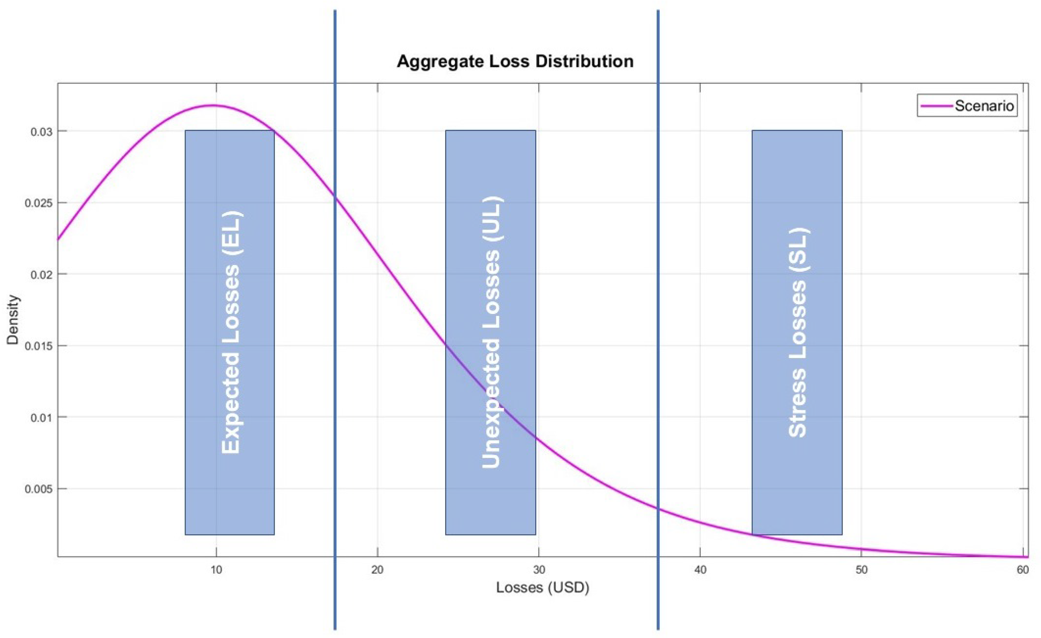
Operational risk (OR) is one of the critical concepts to achieve organizations’ environmental and financial sustainability. According to the Basel II agreement, operational risk (OR) is defined as “…the possibility of incurring in losses due to deficiencies, failures or inadequacies in human resources, processes, technologies, infrastructure or by the occurrence of external events…” [8]. OR has emerged as a key concept for characterising risks arising from phytosanitary and climatic events in agricultural crops and is described by aggregate loss distribution (ALD). ALD groups phytosanitary risk events, such as the suggested LW, into three-loss categories (parametric risks): expected losses (EL-C1 Risk Category), derived from the identification of healthy palms; unexpected losses (UL-C2 Risk Category), derived from the identification of apparently healthy palms; and stress losses (SL-C3 Risk Category), derived from the misidentification of oil palms units with LW in advanced stages. These risk categories make it possible to establish a differentiated treatment of crop units according to LW-affectation (risk parameters), leading to a natural reduction in insecticides and fertilizers. In general, ALD is characterised by slender distributions (log-normal, log-logistic, Weibull, Pareto) [9], where the difference between the EL and SL values represents the sustainability GAP ($S-GAP$). Expanded $S-{GAP}_{\mathrm{s}}$ indicate improved sustainability due to better crop management. The concepts mentioned above were included by the RSPO Standards (Round-table for Sustainable Palm Oil), which aim to improve the environmental sustainability of oil-palm cultivation worldwide [4,10].

This paper proposes a Lagrangian deep-learning model (LG-HDLM) for the spatio-temporal characterisation of early-stage phytosanitary events suggested by LW in oil-palm crops. The LG-HDLM model integrates two sub-structures, a first substructure (Substructure 1) defined by a stacked deep-learning model (SDLM) for identifying and labelling of morphologically complete oil-palm units (MCOPs). The MCOPs were obtained from a segmentation process (cropped images-CIs) carried out on each reflectance band that defines a multi-spectral aerial image (MAI) (green, red, red edge, near infrared) and on three vegetation indices commonly used to assess plant vigour in crops: NDVI (normalized difference vegetation index), GNDVI (green NDVI), and NRVI (normalized red vegetation index) [11]. The MAIs were captured over a study zone using a UAV (unmanned aerial vehicle). A second substructure (Substructure 2) integrates a Convolutional deep-learning model (CDLM) for the spatial characterisation of phytosanitary events (PEs) based on the risk categories that define the ALD. For the report of PEs at an early stage, this layer integrates an inverse Lagrangian Gaussian dispersion model (I-LGPTM) [12] to describe the evolution of LW in the field, creating the structure of a forecast map (dynamic vegetation index).

For the classification of oil-palm crops by risk categories, the LG-HDLM (Substructure 2) integrates a novel Softmax function defined by a generalised Log-logistic activation function. For its analysis and evaluation, two risk scenarios were defined. A first risk scenario (Reference Scenario—Scenario 1) shows the structure of losses for a natural evolution of LW in the field for a period of 6-months. For Scenario 1, the MCOPs were randomly selected and classified by LW-affectation (Scenario 1: EL:744, UL:106, SL:150, month 6). According to the Basel II agreements, this scenario was set up at a reliability of $99.9\%$ (1000 crop units). A second risk scenario shows a projected starting point of disease onset, composed of ten (10) random points of disease dispersion (Scenario 2: EL:840, UL:150, SL:10, month 0—focus of disease). The latter shows the LW evolution in the field for stages before Scenario 1, using an inverse Lagrangian Gaussian puff-tracking model (I-LGPTM) integrated into the convolutional layer that defines Substructure 2. A third risk scenario shows the evaluation metrics based on a spatial LW-affectation (Scenario 3: ELM:855,ULM:144, SLM:1, Metric Scenario), where 855 (ELM) represents the number of oil palms correctly identified by a model in the three risk categories aforementioned (EL–UL–SL), 144 (ULM) crop units in which a model fails to decide, and 1 (SLM) crop unit in which the model fails to detect LW in advanced stages. For this scenario, the sustainability $S-GAP$ of reference is set at a value of $S-GAP$:854 (e.g., $ELM-SLM$).

For the analysis and validation of LG-HLDM in a first stage, LG-HDLM was evaluated against the identification and labelling of MCOPs (Substructure 1) using the CIs per MAI and per VI obtained from the segmentation process aforementioned. This evaluation identifies the reflectance band (Spectral image) or vegetation index (VI) that allows better identification of MCOPs by LW-affectation. In the first phase within a second stage, the LG-HDLM was evaluated against the reconstruction of the loss structure defined by Scenario 1 and was validated against two generalised deep-learning models commonly used for pattern classification and labelling: a deep-learning model with Stochastic stacked structure (SSDL) [13], and a deep-learning model with convolutional structure (CDLM) [14]. In a second phase within the same stage, the LG-HDLM (Substructure 2) was evaluated against three temporal risk scenarios showing the evolution of LW in a study zone for a period of 6 months before reference Scenario (Scenario 2—month 0, Scenario 2.1—month 1, Scenario 2.2—month 2).

In general, LG-HDLM reached performance rates close to $85\%$ on average against the characterisation of MCOPs by LW-affectation for Scenario 1 (ELM:858. ULM:113,SLM:29). This performance was above the performance rates achieved by the SSDL model with $74.4\%$ (ELM:744,UL:106,EL:150) on average and above the performance rates achieved by the CDLM model with $79.4\%$ model (ELM:794,ULM:74,SLM:133) on average for the same scenario. A previous labelling of MCOPs promoted this good performance carried out by Substructure 1 (Stage 1). In this first stage, Substructure 1 achieved values above $90\%$ for an $ACC$-w index (Accuracy weighted index) against the classification of MCOPs by risk category using the CIs obtained from NDVI and GNDVI Indices, which corroborated the importance of these indices for assessing the plant vigour in the field. In a second stage (Substructure 2), the proposed model achieved performance rates close to $80\%$ against the risk characterisation for each temporal scenario defined for this study. This suitable performance resulted in the evolution of ALDs toward lighter losses, widening the sustainability GAP ($S-GAP$) based on Scenario 3 [15]. By its conception, the LG-HDLM model set up a reference model for modelling parametric risks. Due to its capacity for adaption and learning, the LG-HDLM can be extended to characterise different phytosanitary events in oil-palm crops and in other crops, a critical element in achieving the balance between development and sustainability in the framework of the SDA-2030.

This paper is structured as follows. Section 1 presents the main development trends identified in the scientific literature. Section 2 presents the methodology for the analysis and validation of the proposed model will be detailed, while Section 3 presents the results’ analysis and discussion according to the parameters and metrics that define the OR. Section 4 concludes and indicates further studies to balance sustainability and development in the SDA-2030 context, integrating financial-risk and computational-intelligence techniques.

2. Literature Review

Researchers have used different technologies to achieve crops’ financial and environmental sustainability. These include spectral and satellite images [16], and unmanned aerial vehicles (UAVs) for automatic fumigation and fertilization systems [17,18]. Additionally, IoT-IoB (Internet of Things and Beings) platforms for real-time monitoring have performed an essential role [19]. Some authors have applied machine-learning models (ML) combined with the techniques mentioned above to assess risk parameters in agricultural operations. To achieve a balance between sustainability and development in oil-palm crops based on the SDA-2030, four development trends can be identified in the scientific literature [20]:

• A first development trend focuses on the use of multi (MIs) and hyper-spectral (HIs) images for the non-destructive phytosanitary diagnosis of crops in situ [21]. A first group of papers shows how MAIs have helped detect phytosanitary events. As proof of this, ref. [22] identified the impact of Mildiu on leaves in tomato cultivation, and ref. [23] characterised the yellow striation on maize crops. Finally, ref. [24] determined the biochemical characteristics and physiological features of PEs in wheat crops. In this same group, ref. [25] showed how MAIs have been used to assess the productivity of macadamia trees. A second group of papers focuses on MAIs to improve risk management in oil-palm crops. In this way, ref. [26] described the relevance of MAIs and VIs for precision farming in oil-palm crops, ref. [27] described the use of advanced classifiers for the diagnosis of healthy oil-palm units from MAIs. Finally, ref. [28] showed a methodology for the use of MAIs to characterise PEs in different crops. This development trend shows how recent advances in optical remote sensing, including camera systems and spectral data analysis, allow the non-destructive diagnosis of phytosanitary events (PEs), improving the process of detecting diseases in crops. Although satellite images (Sis) are an excellent alternative for the monitoring and characterisation of PEs in oil-palm crops located over large areas of land, the frequency for capturing, the required resolution, and the associated costs for processing these images is a barrier to decision makers [29].
• A second development trend focuses on designing vegetation indices (VIs) using multi-spectral images (MIs). The NDVI (Normalised difference vegetation index) is one of the most cited, e.g., in the area of evaluating the plant vigour in areas of considerable agricultural coverage [30]. This index is also used in combination with others, such as GNDVI (green normalised difference) and SAVI (soil adjusted), to determine plant vigour in vineyards and tomato crops [26]. While some authors have discussed the applicability of MIs for the diagnosis of vegetation states in different agriculture crops [22], others have developed VIs by using just MIs, obtaining satisfactory results. Some researchers have developed VIs based on multi-spectral aerial images (MAIs) taken with unmanned aerial vehicles (UAVs), e.g., for the spatial characterisation of oil-palm crops [27], and for the detection and diagnosis of phytosanitary states in different crops [28]. In addition, these MAIs have been used for the identification of fruits in coffee crops [23], for the treatment of weeds [31] and for the control of deforestation processes [32]. It is essential to highlight the preponderance achieved by the MAIs for diagnosing crop health, overcoming the limitations of SIs in monitoring units for different crops. It is also necessary to highlight the technological development of hyperspectral images (HIs); however, the creation of VIs for the diagnosis of PEs using this technology is still at a very early stage of development [18].
• A third development trend focuses on creating augmented-intelligence platforms (AIPs) to improve the real-time characterisation of crops. These platforms aim to integrate different technologies for the diagnosis of PEs, among which RGB (red-green-blue) and MI images, and ML and DL models, stand out [33,34,35]. Other researchers have pushed these platforms by integrating IoT (Internet of Things) devices, such as optical and multi-spectral sensors and technologies for communication (LORA, Zigbee). In this way, ref. [36] mapped arctic vegetation, ref. [19] showed the ecological monitoring of open-space species, and ref. [37] improved the autonomy of unmanned aerial vehicles (UAVs), identifying disease hot spots located over large areas of crops, supported by ML and DL models. Within ML and DL modelling to support AIPs in monitoring crops, ref. [38] presented a convolutional neural model (CNN) to detect pine trees affected by wilt using MAIs, and ref. [39] presented a set of ML algorithms to improve irrigation process in vineyards also using MAIs. Finally, ref. [40] presented a preliminary analysis of pathology detection in oil-palm crops using convolutional neural networks (CNN) integrating MAIs and VIs. Finally, ref. [40] presents a preliminary analysis of pathology detection in oil-palm crops using convolutional neural networks (CNN) integrating MAIs and VIs. This development trend shows how AIPs have enabled efficient real-time crop management by integrating IOT technologies. However, it can be observed that there is an absence of AIPs that integrate models for adaptation and learning to identify the dispersion dynamics or for the characterisation of risks derived from a PE in crops.
• A fourth development trend focuses on the design of parametric insurances based on the characterisation of operational risk (OR) for different management scenarios [41]. Within this trend, the first group of studies shows how the ML concepts have been used to model OR [42]. Some researchers have defined fuzzy-inference models for the qualitative description of scenarios for OR management [8] or to determine the inherent risk as a result of implementing different management scenarios when mitigating OR [43]. In addition, the estimation of this risk through the integration of multi-dimensional databases is available in [9]. Within this trend, a second group of studies focuses on the configuration of parametric insurances in developing countries [44]. The first study presents a series of recommendations to achieve the sustainability of oil-palm crops through the characterisation and identification of operational and reputational risks [45]. In contrast, a second study shows the configuration of parametric insurances concerning risk related to changing weather conditions [46]. Furthermore, it has been demonstrated how insurance contracts can be designed based on a farmer satisfaction index by integrating statistical analysis of agro-climatic data and by applying optimisation techniques for improving the coverage for catastrophic risks [47]. Ref. [48] shows how neural networks have been used for credit-risk modelling by analysing the relationship between access to credit and productivity in the agricultural sector for a large set of countries. Due to the importance of OR in the design of insurance products for the protection of farming activities, in this development trend, as in the case of the previous trend, it is observed that there is an absence of models integrating ML and financial-risk concepts for the improvement of the environmental and financial sustainability of crops [20].

The development trends described above generally aim to improve the environmental and financial sustainability of global agricultural activities through the integration of technologies. It is essential to note that financial risk has emerged as a critical element in improving organisations’ environmental and economic sustainability in recent years, becoming one of the most promising concepts for improving the sustainability of crops. The literature review also shows the absence of models to characterise the dynamic of a PE in the field and risk models to reduce the impact of a PE integrating financial indicators. In this context, the integration of technologies for the efficient management of risks derived from a phytosanitary or agro-climatic event (PAE) could have a direct effect on a natural reduction in insecticides and fertilisers, helping, in a decisive way, to achieve the balance between development and sustainability pursued by the SDA-2030 [1].

2.1. Theory And Definitions

2.1.1. Operational Risk

According to the Basel II agreement, operational risk (OR) is defined as: “…the possibility of incurring in losses due to deficiencies, failures or inadequacies, in human resources, processes, technologies, infrastructure by the occurrence of external events…”. OR groups all risks associated with an organisation’s business activities and is described by the aggregate distribution of losses (ALD) [8,9,43].

OR is a concept that has been widely used to characterise the risks associated with an organisation’s business operations. In recent years, this concept has been extended to the improvement of financial and environmental sustainability of farming activities, giving rise to the concept of parametric risks, which are the basis for the coverage of crops through the use of index insurance policies [47].

2.1.2. Aggregate Loss Distribution (ALD):

Aggregate loss distribution (ALD) groups the risks associated with an organisation’s business activities into three loss categories (Figure 1) [49]:

• Expected losses (EL): EL losses are known as predictable losses and represent the group of losses that an organisation can assume. The mean of the ALD establishes the upper limit for this type of losses.
• Stress losses (SL): SL refers to the group of losses that generate a significant deterioration of the assets of an organisation (catastrophic or restorative losses). The operational value at Risk (OpVar) represents these losses, which is located at the $99.9\%$ percentile of the ALD. The OpVar represents the insurable value to protect the assets of an organisation.
• Unexpected losses (UL): UL refers to the group of losses that are located between the EL limit and the OpVar value. These losses are known as manageable losses.

The ALD distribution has the following characteristics:

• In general, the ALD is represented by long-tailed probability distributions, among which the most prominent are: log-logistic, log-normal, Weibull or generalised Pareto [9,43].
• In the context of oil-palm crops, an event risk is quantified as the convolution between the frequency (number of crops affected by LW) and the severity (cost of eradication and treatment of oil palm units, e.g., insecticides) in a period (usually one day).
• The difference between EL and SL losses leads to evaluating the environmental and financial sustainability of crops affected by a phytosanitary or an agro-climate event (sustainability GAP ($S-GAP$)).
• Under the Basel III agreement, the ALD distribution is known as the loss component (LC) [50].

2.1.3. Log-Logistic Distribution

The log-logistic distribution (known as the Fisher distribution) is a continuous probability distribution for modelling a non-negative random variables. The flexibility of this distribution, makes it ideal for the classification of loss events using adaptive and learning models according to the ALD structure. The log-logistic distribution can be handled as an activation function of the Softmax class [51,52], and can be expressed as shown in (Equation (1)).

$$z_{jc}=\frac{1}{1+{\left(\frac{y{s}_{j_c}-a}{\alpha }\right)}^{-\beta }}$$

(1)

where:

• $z_{jc}$ represents the cumulative probability distribution (CDF) for a risk category $j_c$.
• $\alpha$: dimensional factor (dcale parameter).
• $\beta$: structural factor (shape parameter).
• a: stability factor (lower limit for the mean).

The log-logistic function is widely used for characterising risks derived from an organisation’s business operations. For the particular case of this study, the log-logistic function will be used as an activation function, which will allow the classification of PEs (phytosanitary events), taking as a reference the structure of the ALD. It is essential to mention that this activation function will evaluate the LG-HDLM stability (structural, dimensional) against the configuration by adaptation and learning of the risk structure generated by the evolution of a PE in the field, maintaining at all times the loss structure that defines the OR.

3. Materials and Methods

Operational risk (OR) has become one of the most promising concepts for configuring risk parameters in crops affected by a PAE. The different loss categories that define the ALD make it possible to establish differentiated insurance coverages to protect farming activities. Despite the development of precision agriculture, widening the environmental and financial sustainability ($S-GAP$) of crops affected by a PAE is still a challenge from a technological perspective. Thus, we propose the following methodology.

3.1. Experimental Study Design

For the characterisation of OR in oil-palm crops affected by lethal wilt (LW-affectation), an oil palm crop that comprises a total of 3500 ha was used (study zone). Two types of oil palms stand out: the African palm $(\mathit{Elaeis} \mathit{guinensis})$ and the American palm $(\mathit{Elaeis} \mathit{oleifera}$-OxG) [53]. To describe the behaviour of LW in the field, a series of multi-spectral images using an unmanned aerial vehicle (UAV) of DJI Phantom 4 series [54] equipped with a Sequoia Parrot multi-spectral camera were captured [55]. The latter device captures multi-spectral aerial images (MAIs) at low heights using four reflectance bands: green (550 nm ± 40 nm), red (660 nm ± 40 nm), red edge (735 nm ± 40 nm), and near infrared (790 nm ± 40 nm), for a resolution of 13 cm/px at maximum height of 120 m. According to the structure of an oil-palm crop (1 ha-144 cultivation units-tres-bolillo arrangement) [56], the MAIs were obtained at a height of 50 m (height of reference) to keep the balance between UAV autonomy and MAIs resolution. Each MAI achieved a coverage of $4200{\mathrm{m}}^2$, for a resolution of 1.2 Mpx (1280 px × 960 px) per band, grouping approximately 60 crop units (Figure 2).

For this study, eight (8) flights were carried out in the study zone with the presence of oil-palm units in an adulthood stage of the species Elaeis guinensis. For each flight, a total of 80 MAIs were captured, reaching a total of 640 MAIs ($8flights\times 80MAIS$). To assess the prevalence of a PE in the field, as suggested by the LW, we proceeded to construct three vegetation indexes commonly used to evaluate the plant vigour of crops in general, based on the reflectance bands that define a MAI: NDVI (normalised difference vegetation index—Figure 3), GNDVI (green NDVI), and NRVI (normalised red vegetation index) [11]. Each MAI and VI was subjected to a segmentation process, taking as a reference a mesh size of 300 px × 300 px (standard size for an MCOP at the height of 50 m), with an overlap of 50 px per dimension. For each MAI or VI, a total of approximately 400 cropped images (CIs) were obtained, where approximately 100 CIs were classified as MCOPs, and the remaining ones (300) correspond to partial oil-palm crops (non-MCOPs) (Figure 3). The total number of MCOPs amounts to 16,000 per month ($80MAIs\times 100CIs\times 2flights$). Finally, and based on phytosanitary censuses carried out in the field for the period covered by this study, the set of MCOPs were grouped into healthy palms (EL), apparently healthy palms (UL), and oil palm units affected by LW (SL) [26,28,30].

For the analysis and validation of LG-HDLM, a risk scenario by random sampling of the total of MCOPs available for month six was created (Reference Scenario—Scenario 1). This sampling process was performed at reliability of $99.9\%$ according to Basell II agreements, and where each of the MCOPs was classified by LW-affectation in each loss category that defines the ALD distribution (

Table 1. Structure of losses for the reference scenarios.

	Scenario 3	Scenario 1
Scenarios	Metric	Reference
Hectares (Ha-Oil Palm Units)	6.9 (1000)	6.9 (1000)
Structure of losses EL-UL-(SL)	856-143-(1)	744-106-(150)
Category 1 (SL-USD)	5580	4136
Category 2 (UL-USD)	3053	5849
Category 3 (EL-USD)	301	45,135
Sustainability GAP	855	594

). Table 1 also shows a reference scenario that groups a series of metrics for the evaluation of a LG-HDLM against the characterisation of risks derived from a PE, such as suggested by LW in the field (Metric Scenario—Scenario 3). This scenario indicates that the misclassification of a MCOP affected by LW (SLM-1) can eradicate approximately one hectare of the crop (ULM-144). In contrast, the ELM metric indicates that a model used for risk characterisation must achieve, at minimum, effectiveness in the classification of MCOPs by loss category close to $85\%$ on average (ELM-855).

3.2. Adaptive Inverse Lagrangian Gaussian Model

To describe the spatio-temporal behaviour of early-stage LW, a dispersal model inspired by an Inverse Lagrangian Gaussing puff-tracking dispersion model (I-LGPTM), widely used for the dispersal of pollutants in the atmosphere, is proposed. The I-LGPTM integrates two dynamics: a first dynamic establishes the dispersion patterns of LW in the field from a focus on disease dispersal, while a second dynamic shows the degree of LW-affectation of each of the palm cultivation units affected by this pattern [12,27,57,58].

3.3. Dispersion Pattern (Dynamic 1)

According to the first dynamic, the dispersion pattern is denoted and defined:

$$Q{m}_{x,y}=\frac{1}{{\left(2.\pi \right)}^{\frac{3}{2}}{\sigma }_{xy}^2}Exp\left(-\frac{1}{2}{\left(\frac{x_f-x}{{\sigma }_{xy}}\right)}^2-\frac{1}{2}{\left(\frac{y_f-y}{{\sigma }_{xy}}\right)}^2\right)$$

(2)

where:

• $Q{m}_{x,y}$ indicates the intensity of LW at the point $\left(x,y\right)$ (m).
• $x_f,y_f$ indicates the location of the focus within the pattern of dispersion (m).
• ${\sigma }_{xy}$: dispersion coefficient that indicates the area of influence of LW in the field from a focus of the disease $\left(x_f,y_f\right)$ (m).

To describe the normalised disease evolution in the field, this coefficient is denoted and defined in the context of a Lagrangian dispersion model as follows:

$${\sigma }_{xy}=e^{-\left(\frac{1}{a.x^{-b}}\right)}$$

(3)

where:

• x: diameter measured from the point of location of the dispersion pattern $(x_p,y_p)$ taking as reference one hectare (ha) of crop (m).
• $a,b$: dispersion parameters that describe the evolution of LW in the study zone (LW-affectation). Figure 4 shows the upward curves of LW dispersion for different dynamics.

According to the scientific literature, this dispersion coefficient was standardised by taking into account the following parameters [4,59]:

• To achieve reliability of $99.9\%$ in the characterisation of LW-affectation in the field, a total of $6.9$ ha ($144\mathrm{un}/\mathrm{ha}\times 6.9\mathrm{ha}=1000\mathrm{un}$) were taken as reference. Based on a circular dispersion pattern, the linear radius of coverage will be close to 150 m (70,685.82 ${\mathrm{m}}^2=\pi .{\left(150\mathrm{m}\right)}^2$).
• For the configuration of the disease focus, a canopy ring consisting of 12 crop units was taken as a reference. This canopy ring has an approximate linear radius coverage of 10 m ($x\left(\mathrm{m}\right)$).
• For stability of the model against the identification and characterisation of LW in the field, this dispersion coefficient performs an automatic normalisation process against disease progress (upward curves).
• To model the dispersion of LW in the field, a disease development rate of $0.0833\mathrm{un}/\mathrm{year}$ (r) was taken as reference for an approximate lot size of $25\mathrm{ha}$ ($144\mathrm{un}/\mathrm{ha}\times 25\mathrm{un}=3600\mathrm{un}$).
• To achieve a theoretical lot coverage for LW, a period of (6) months was taken. For this period, the rate of disease (r) development resulted in approximately $150\mathrm{un}$ affected crop units, as described in the reference (Scenario 1).

3.4. LW-Affectation (Dynamic 2)

A second dynamic integrates an inverse dispersion mechanism to model the LW-affectation of MCOPs given a dispersion pattern (Dynamic 1). The LW-affectation for each MCOP is modelled through the use of Gaussian functions, where the downward curves (Figure 4) show the compression of MCOPs due to an unusual concentration of energy by leaflet necrosis. According to the morphological structure of each crop unit (MCOP unit), this dispersion factor is denoted and defined:

$$MCO{P}_{x,y}=\frac{Q{m}_{x,y}}{{\left(2.\pi \right)}^{\frac{3}{2}}.{\sigma }_{xy,p}^2}Exp\left(-\frac{1}{2}{\left(\frac{x_p-x}{{\sigma }_{xy,p}}\right)}^2-\frac{1}{2}{\left(\frac{y_p-y}{{\sigma }_{xy,p}}\right)}^2\right)$$

(4)

where:

• $MCO{P}_{x,y}$: LW-affectation of the point $\left(x,y\right)$ given a dispersion pattern $Q{m}_{x,y}$.
• ${\sigma }_{xy,p}$: Compression coefficient (inverse dispersion) for an MCOP located at the point $\left(x_p,y_p\right)$. This compression coefficient is denoted and defined as follows:

  $${\sigma }_{xy,p}=-ks.\left(\frac{1}{a.x^{-b}}\right)$$

  (5)

where:

• $ks$ indicates the size of an MCOP in the standardised space (Study Zone). According to the initial size of the dispersion pattern ($Q{m}_{x,y}$), an MCOP will have a length approximately of $10\%$ ($ks=0.4\times 10\%$) of the spatial coverage by this pattern.

Figure 5 shows the behaviour of the Gaussian-MCOP functions for different LW-affectation levels (compression curves). Here, the MCOPs that have slender Gaussian structures (Figure 5c) and present a higher LW-affectation than those MCOPs that have Gaussian functions with more extended structures (Figure 5a). This higher compression generates higher LW-affectation, as specified by the negativity reached by the dispersion coefficient b.

According to risk scenarios defined by this study, Figure 6 shows the normalised spatial behaviour of LW for a risk scenario before the reference scenario. The dispersion pattern affecting the MCOPs present in the study area can be observed in the lower-left part. It is essential to mention that the Gaussian-MCOP functions close to the focus of dispersion present more slender structures (upper-right figure) due to compression, which causes necrosis of the palm leaflets. The lower-right figure shows the structure of the forecasting map describing the evolution of LW in the field, based on the dispositioning (tres-bolillo arrangement) of cultivation units shown in Figure 2.

3.5. Lagrangian Hybrid Deep-Learning Model (Lg-Hdlm)

For the characterisation of the risk arising from the phytosanitary and agro-climatic event (PAE) in agreeing to the structure of losses defined by ALD, a Lagrangian hybrid deep-learning model $(LG$-$HDLM)$ is proposed. Two substructures describe the structure of the model: The first one integrates a stacked deep-learning model for the identification and labelling of MCOPs (Substructure 1) from MAIs and VIs. In contrast, the second one integrates a convolutional Lagrangian Gaussian deep-learning model to characterise the risks derived from the spatio-temporal evolution of LW in the field (Substructure 2).

3.5.1. Stacked Deep-Learning Structure (Substructure 1)

For the identification and labelling of MCOPs (Figure 3), the first substructure is inspired by a neural network with a stacked deep-learning structure [60], which is denoted and defined (Equation (2)):

$$h_{j_n,k}=\left(\sum _{\begin{array}{c}{j}_n=1\end{array}}^{n{o}_n}{w}_{j_n,j_{n-1},k}\dots \left(\sum _{\begin{array}{c}{j}_2=1\end{array}}^{n{o}_2}{w}_{j_1,j_2,k}\left(\sum _{\begin{array}{c}{j}_1=1\end{array}}^{n{o}_1}\sum _{\begin{array}{c}{j}_0=1\end{array}}^{n{o}_0}\left(w_{j_1,j_0,k}.x_{j_0,k}\right)\right)\right)\right)$$

(6)

where:

• $x_{j_0}$ represents the input vector or k cropped image (CI) ($k=1,2,\dots ,ND$). Each of the CIs has a size of $\left(300\mathrm{px}\times 300\mathrm{px}\right)$ per MAI or VI.
• $ND$ represents the number of CIs available for the configuration of the model.
• $w_{j_n,j_n-1}$ represents the neural connections between the $j_n$ and the $j_{n-1}$ layer.
• $n{o}_n$ indicates the number of hidden elements or neurons that make up the n layer.
• $h_{j_n}$ represents each of the $j_n$ outputs of the $n{o}_n$ neurons that make up a hidden n layer.

The number of neurons that make up each stacked layer can be estimated [61]:

$$n{o}_n=n{o}_{max}-ni\left(\frac{n{o}_{max}}{nl}\right)$$

(7)

where:

• $n{o}_n$: number of hidden neurons for the n$layer$.
• $nl$: number of stacked layers (cardinality) ($n=1,2,\dots ,nl$).
• $n{o}_{max}$: maximum number of neurons for the $1st$$layer$ (compression ratio).

For the configuration of stacked-layers structure, the following set-up metrics are proposed:

• Cardinality: Indicates the number of stacked layers that make up a deep-learning neural model of the stacked type. Higher cardinality leads to greater flexibility in modelling complex systems, bringing higher computational costs.
• Compression Ratio: Indicates the compression capacity of each layer that makes up a neural deep-learning model by stacked layers when configured using auto-encoder strategies. The compression ratios performed by the first stacked layer for these models determine its behaviour in modelling complex systems.

According to an autoencoder learning strategy, each of the layers that make up this substructure can be expressed as follows [60]:

$$x_{j_{n_l-2},k}=\sum _{\begin{array}{c}{j}_{n_l}=1\end{array}}^{n{o}_{n_l}}{w}_{j_{n_l}{j}_{n_l-1}.k}.\left(\sum _{\begin{array}{c}{j}_{n_l-1}=1\end{array}}^{n{o}_{n_l-1}}\sum _{\begin{array}{c}{j}_{n_l-2}=1\end{array}}^{n{o}_{n_l-2}}\left(w_{j_{n_l-1}{j}_{n_l-2},k}.x_{j_{n_l-2},k}\right)\right)$$

(8)

The autoencoder learning strategy can be expressed in terms of the generalised delta rule as follows (3) [62]:

$$w_{j_{n_l}{j}_{n_l-1},k}=w_{j_{n_l}{j}_{n_l-1},k-1}-\alpha .\frac{\partial e_{j_{nl-1},k}^2}{\partial w_{j_{n_l}{j}_{n_l-1}}}$$

(9)

where:

• $e_k^2$ represents the mean square error (e.g., mse), which is expressed as:

$$e_{j_{nl-1},k}^2=\frac{1}{ND}\sum _{\begin{array}{c}j=1\end{array}}^{ND}{\left(x_{j_{n_l-1},k}-x_{j_{n_l-1},k}\right)}^2$$

(10)

where:

• $x_{j_{n_l-2},k}$: Represents the input and output values used as a reference for the configuration of the $n_l$ hidden layers that build the stacked structure of the proposed model.

The fully connected layer (FCL) can be expressed as follows:

$$z_{j_c}=\sum _{\begin{array}{c}{j}_{n_l}=1\end{array}}^{n_{n_l}}{c}_{j_c,j_{n_l}}.h_{j_{n_l}}$$

(11)

where:

• $c_{j_c,j_{n_l}}$ represents the FCL connections.

For the identification and labelling of MCOPs, the Softmax function can be expressed [63]:

$$S_m=\sum _{\begin{array}{c}{j}_c=1\end{array}}^{n_c}{e}^{z_{j_c}}$$

(12)

$$\sigma \left(z_{j_c}\right)=\frac{e^{z_{j_c}}}{S_m}$$

(13)

where:

• $j_c$: labelling categories (MCOP, non-MCOP) $j_c:1,2,\dots ,k_c$.
• $z_{j_c}$: probability associated with a $j_c$$category$.

3.5.2. Convolutional Lagrangian Gaussian Deep-Learning Model (Substructure 2)

For the spatio-temporal characterisation of phytosanitary events in crops in general, we propose Substructure 2 inspired by a convolutional deep-learning model. This substructure integrates an I-LGPTM to describe the evolution of a phytosanitary event (LW-affectation) in stages before a temporal reference scenario (forecasting maps—Equations (2) and (4)). The convolutional layer can be described as follows:

$$FCM\left(x_j,y_j,k\right)=\frac{1}{{\left(2.\pi \right)}^{\frac{3}{2}}{\sigma }_{x,k}.{\sigma }_{y,k}}.e^{\left(-\frac{1}{2}.{\left(\frac{X{C}_{j,x}-x_{j,k}}{{\sigma }_{x,k}}\right)}^2-\frac{1}{2}{\left(\frac{X{C}_{j,y}-y_j}{{\sigma }_{y,k}}\right)}^2\right)}$$

(14)

where:

• $X{C}_{j,x},X{C}_{j,y}$: relative position for a j$crop$ unit in the field.
• $x_{j,k},y_{j,k}$ indicates the spatio-temporal spread of LW from a j crop unit and a k $instant$ time.
• ${\sigma }_{j,x,k},{\sigma }_{j,y,k}$: Dispersion coefficients that determine the dynamic of LW-affectation from a $X{C}_{j,x,k},X{C}_{j,y,k}$ spatial point. These coefficients can be modelled based on phytosanitary censuses for LW-affectation carried out in the field for the period defined for this study.

Substructure 2 integrates a convolutional mechanism, where MCOP-Gaussian functions define the convolutional patterns. In this way, this convolutional mechanism can be defined as a functional macro-convolutional mechanism as follows:

$$\mathsf{\Phi }\left(x_{j,k},y_{j,k},l\right)=\left[\varphi {\left(FC{M}_{x_j,y_j,l,k}.MCO{P}_{x_{j_r},y_{j_r},l,j_c,k}\right)}_{j_{ic}}\right]$$

(15)

where:

• $\mathsf{\Phi }\left(x_{j,k},y_{j,k},l\right)$: Vector of agreement indices between a Gaussian-MCOP pattern ($j_c$ risk category) for each of the points ($x_{j,k},y_{j,k}$) that make up a l convolutional layer (IC-fingerprint).
• $MCO{P}_{x_{j_r},y_{j_r},l,j_c,k}$: Convolutional Gaussian-MCOP pattern for a l MAI or l VI, a $j_c$ risk category for a k instant time. The convolutional Gaussian-MCOP patterns will be selected from Scenario 1 by LW-affectation.
• $j_{ic}$ represents the $j_{ic}$ agreement index. For the characterisation of oil-palm units by LW-affectation based on Gaussian-MCOP patterns, we propose the following agreement indices [64]:
  • $IO{A}_{l,k}$: Index of agreement between a spatial oil palm and a $MCO{P}_{x_{j_r},y_{j_r},l,j_c,k}$ convolutional pattern.
  • $M{G}_{l,k}$: Geometric mean bias between a spatial oil palm and a $MCO{P}_{x_{j_r},y_{j_r},l,j_c,k}$ convolutional pattern.
  • $V{G}_{l,k}$: Geometric variance bias between a spatial oil palm and a $MCO{P}_{x_{j_r},y_{j_r},l,j_c,k}$ convolutional pattern.

According to Equation (15), Figure 6 exhibits the spatial analytical structure of a set of oil-palm units that are located in the study zone. Here, we can observe that the Gaussian-MCOPs, with smaller diameters, show a higher energy concentration in the centre (low spatial variance) due to the necrosis of the plant’s leaflets. This fact generates an unusual concentration of the greatest plant vigour points. However, the Gaussian bells with a larger diameter (high spatial variance) present a greater energy dispersion due to the homogeneous spatial dispersion of plant vigour in healthy oil-palm units.

For the classification of palm cultivation units in each of the loss categories defined by ALD (EL,UL,SL), the fully connected layer (FCL) can be defined as follows:

$$z_{j_c}=\sum _{\begin{array}{c}{j}_{ic}=1\end{array}}^{n_i}{c}_{j_c,j_{ic}}.\mathsf{\Phi }{\left(x_{j,k},y_{j,k},l\right)}_{j_{ic}}$$

(16)

$${\sigma }_{LLG}\left(z_{j_c}\right)==\frac{1}{1+e^{-\frac{\alpha .\left(x-a\right)}{\beta }}}$$

(17)

$${\sigma }_{LLG}\left(z_{j_c}\right)=Softmax\left(z_{j_c}\right)$$

(18)

where:

• ${\sigma }_{LLG}\left(z_{j_c}\right)$: log-logistic Softmax function for the classification of crop units in the $j_c$ risk category (Equation (13)).
• $c_{j_c,j_{ic}}$: Represents the FCL connections for a $j_c$ risk category and $j_{ic}$ index of agreement.

3.6. Metrics

For the analysis and validation of LG-HDLM against the identification and characterization of the risk derived from a phytosanitary event (PE) such as that suggested by LW, we propose the following metrics in agreement with ALD loss structure:

3.6.1. Accuracy Weighted Index (Acc-w)

Accuracy weighted index shows the general behaviour of a model against the classification of patterns:

$$Ac{c}_w=\frac{{\displaystyle \sum _{i=1}^{j_c}}{w}_{j_c,p}T{P}_{j_c}+{\displaystyle \sum _{i=1}^{j_c}}{w}_{j_{c}n}T{N}_{j_c}}{{\displaystyle \sum _{i=1}^{j_c}}\left(T{P}_{j_c}+T{N}_{j_c}\right)}$$

(19)

where:

• $w_{j_c}$ represents the weighted effect of the number of data that belongs to a category $j_c$.
• $T{P}_{j_c}$: true positive number of data that are correctly identified by a model for a $j_c$ category.
• $T{N}_{j_c}$: true negative number of data that are erroneously identified by a model for category $j_c$.

According to the set of CIs available for the configuration of Substructure 1, this index will allow evaluating the performance of LG-HDLM against the classification and labelling of CIs based on the ratio defined for the categories of MCOPs and non-MCOPs by reflectance band and VI.

3.6.2. Categorical Cross Entropy (CCE)

Categorical cross-entropy is a loss function that compares the probability distribution of the predictions (${\widehat{y}}_k$) with the probability distribution that represents the data of reference ($y{d}_k$), as we have two classes (EL (healthy palms), SL (LW-affected palms)). CCE can be defined as follows:

$$L=-\frac{1}{ND}\sum _{\begin{array}{c}k=1\end{array}}^{ND}\left[y{d}_{k}log\left({\widehat{y}}_k\right)+\left(1-y{d}_k\right)log\left(1-{\widehat{y}}_k\right)\right]$$

(20)

where:

• ${\widehat{y}}_k$: Represents the value predicted by the model for observation k.
• $y{d}_k$: Value of reference or desired value for observation k.
• $ND$: Total of samples of data or MCOPs available ($k=1,2,3,\dots ,ND$).

According to the substructures that make up the LG-HDLM, this metric will evaluate the model’s performance against the following criteria:

• For classification and labelling, this metric will allow evaluating the performance of the LG-HDLM (Substructure 1) against the classification and labelling of CIs in the categories of MCOPs and non-MCOPs reflectance band and VI.
• For the discrete-risk classification, this metric will allow evaluating the performance of LG-HDLM (Substructure 2) against the classification of MCOPs by loss category, according to the loss structure defined by ALD.
• For the continuous-risk characterisation, this metric will assess the stability of LG-HDLM against the characterisation of ALD structure by risk scenario, according to the probabilities assigned by the Softmax function for each of the MCOPs classified by risk category.

3.7. Dimensional and Structural Stability

To analyse the stability in models by adaption and learning about the characterisation of loss structure that defines the ALD for a PE, such as the one suggested by LW, four statistical indices were taken as reference [64]: index of agreement (IOA), which quantifies the intensity of the linear relationship between the reference losses and the estimated losses for EL category; the variance (VC), which allows assessing the impact of UL about the mean of ALD; the skewness coefficient (SK), which shows the evolution of the ALD distribution towards lighter losses; and the kurtosis coefficient (KC), which assess the evolution of losses towards the EL category.

Concerning learning stability, structural Stability (SS) indicates the ability of a model by adaption and learning to reconstruct the loss structure that defines the ALD for Scenario 1 [20]. To achieve this stability, LG-HLDM is expected to reach IOA values close to $95\%$ on average and similar values in terms of VC, SK, and KC. Regarding dimensional stability, it shows the stability of a model to the magnitude of losses for a baseline scenario (Scenario 1). To achieve this stability, the SK and KC indices are expected to increase. At the same time, for the variance, losses will increasingly cluster in the EL category, as the ALD groups losses with a smaller magnitude due to better risk management. This will result in lean probability distributions with increasingly lighter loss structures and extended GAPs.

3.8. Mean Square Error (mse)

The mean square error (mse) measures the average of the squared errors of the estimated values ${\widehat{y}}_{j_c,k}$ and the desired values $\widehat{y{d}_{j_c,k}}$ of a model.

$$mse=\frac{1}{ND}\sum _{k=1}^{ND}{\left(y{d}_{j_c,k}-{\widehat{y}}_{j_c,k}\right)}^2$$

(21)

where:

• $y{d}_{j_c,k}$: indicates the reference values to set-up and adaptive models for k$record$ and $j_c$ $category$.
• ${\widehat{y}}_{j_c,k}$: indicates the value estimated by an adaptive model for k$record$ and $j_c$ $category$.

For the classification of MCOPs, the $mse$ emerges as a measure showing the risk of loss of sensitivity of the LG-HDLM.

3.9. Experimental Validation

For the experimental validation of LG-HDLM, two stages were considered. In the first stage, the model was evaluated against the identification and labelling of MCOPs (Substructure 1): a total of 640 MAIs (four reflectance bands) ($8flights\times 80MAIS$) and 1920 VIs grouped in three categories: GNDVI ($640\mathrm{un}$), NDVI ($640\mathrm{un}$), and NRVI ($640\mathrm{un}$) were available (7) databases. Each of these databases represents the natural evolution of LW in the field for a period of time of 6 months. Each MAI and each VI were subjected to a segmentation process, taking as a reference a mesh size of $300\mathrm{px}\times 300\mathrm{px}$ (cropped image size (CI)—MCOP at a height of 50 m), with an overlap of 50 px per dimension. This process yielded a total of 400 CIs per reflectance band and per VI ($100MCOPs300non-MCOPs$), which were classified into MCOPs (64,000 un) and non-MCOPs (192,000 un). Substructure 1 was configured at a reliability of $99,9\%$ under the Basel II Agreements [61], so it was necessary to define a total of 1000 learning cycles, and a random sampling per cycle of 1000 CIs on the classification categories (MCOP, non-MCOP) per database. For each learning cycle, the data were grouped into training ($70\%$) and validation data ($30\%$). In contrast, for the learning generalisation (in the absence of a learning process), a total of 1000 additional random CIs were used. Substructure 1 was set-up sequentially using aautoencoder strategy to a maximum cardinality of ten (10) stacked layers. In this stage, it is expected that LG-HDLM will achieve a balance between the compression ratios and the cardinality in the identification and labelling of MCOPs. Likewise, this configuration is expected to achieve $ACC$-w performance values close to $90\%$ on average, as well as values close to zero (0) for mse and CCE metrics.

Two phases were considered for the experimental validation of LG-HDLM against the risk characterisation (Stage 2). In the first phase, the proposed LG-HDLM was evaluated against the risk characterisation for the reference scenario (Scenario 1), whereby the LG-HDLM was expected to yield probability distributions with slender structures, similar to the reference probability distributions used for ALD modelling such as log-normal, log-logistic, Weibull or Generalised Pareto (structural stability in learning) [9]. The stability of the model against the characterisation of the loss structure was performed using the IOA index and the negative log-likelihood (CCE Continuous-NLogL). Here, Substructure 2 is expected to yield IOAs close to $100\%$ regarding the loss structure defined for each Scenario. At the same time, the selection of the distribution will be carried out against the goodness of fit, taking as reference the lowest NlogL. In this same stage, two generalised neural models with deep-learning structures, which had been widely used for pattern identification and classification, were used to validate the model: a stochastic neural model with a stacked deep learning structure (SSDL) [14] and a convolutional deep-learning neural network (CDLM) with stochastic computing [13]. In the validation stage, LG-HDLM was expected to yield probability distributions with extended S-${GAP}_{\mathrm{s}}$, and performance indices higher than $75\%$ on average ($ELM$-$750\mathrm{un}.$) against the classification of MCOPs by risk category and for each of the scenarios. The ALDs were also expected to have slender structures with lighter losses, to ensure the structural and dimensional stability of LG-HDLM against the risk characterisation. The loss structure was financially assessed based on the costs related to the management, treatment and eradication of MCOPs affected by LW in nonproductive stages of oil palms (year 1–year 2) [4,7].

In a second phase (within Stage 2), three temporal risk scenarios describing the evolution of LW in the field for a previous period of 6 months before Scenario 1 were created (

Table 2. Structure of losses for the reference scenarios.

	Scenario 3	Scenario 1	Scenario 2.2	Scenario 2.1	Scenario 2
Scenarios	Metric	Reference	Month 4	Month 2	Month 0
Hectares (Ha-Oil Palm Units)	6.9 (1000)	6.9 (1000)	6.9 (1000)	6.9 (1000)	6.9 (1000)
Structure of Losses EL-UL-(SL)	856-143-(1)	744-106-(150)	792-130-(78)	801-165-(34)	840-150-(10)
Probability Distribution	log-logistic	log-logistic	log-logistic	log-logistic	log-logistic

). These risk scenarios were obtained by inverse spatio-temporal modelling, using the I-LGPTM that integrates the convolutional mechanism defined by Substructure 2. The patterns (MCOP-patterns) that trigger the convolutional mechanism against the classification of MCOPs by LW-affectation were randomly selected from the MCOPs grouped in Scenario 1. This random selection was set at $5\%$ of the total of MCOPs available per risk category. For the evaluation of LG-HDLM (Substructure 2) against the risk characterisation by LW-affectation, an IC fingerprint composed of three agreement indices related to each risk category is proposed: IOA (index of agreement), MG (geometric mean bias), and VG (geometric variance bias) [64]. Regarding the IC fingerprint, LG-HDLM is expected to achieve agreement values above $90\%$ on average to ensure that the classified MCOPs possess the same structural characteristics as the convolutional MCOP patterns used. Regarding the risk characterisation, LG-HDLM is also expected to achieve performance indices above $85\% \left(ELM\right)$ on average against the classification of MCOPs in the risk categories defined by each temporal scenario (structural stability). Sustainability S-${GAP}_{\mathrm{s}}$ are expected to be above $80\%$ on average to ensure the environmental and financial sustainability of oil-palm crops from the configuration of risk parameters (dimensional stability) in the early stages of the onset of LW based on SDA-2030 criteria.

4. Results

Table 3. Behaviour of Substructure 1 in the identification and labelling of MCOPs based on reflectance bands.

	NIR			REG			RED
	Train	Val.	Gen.	Train	Val.	Gen.	Train	Val.	Gen.
ACC/-w	0.6667	0.5333	0.5012	0.4667	0.3333	0.54126	0.4253	0.3333	0.5526
CCE	5.3727	7.5218	8.1253	8.5963	10.7454	11.2356	8.8563	10.7636	11.2556
MSE	0.4667	0.3333	0.4512	0.5333	0.6667	0.5443	0.5512	0.8667	0.9264

and

Table 4. Behaviour of Substructure 1 in the identification and labelling of MCOPs based on VIs.

	NDVI			GNDVI			NRVI
	Train	Val.	Gen.	Train	Val.	Gen.	Train	Val.	Gen.
ACC-w	0.9933	0.9188	0.9933	0.9733	0.7667	0.9933	0.4667	0.3333	0.4666
CCE	0.0665	0.0140	0.0398	0.1030	0.8506	0.0643	8.9563	10.7454	8.59631
mse	0.0140	0.2198	0.0056	0.0206	0.2596	0.0086	0.5333	0.6667	0.5333

show the performance achieved by LG-HLDM (Substructure 1) against the identification and labelling of MCOPs for three near-infrared reflectance bands (red, red edge, near infrared) and three VIs (NDVI,GNDVI,NRVI) commonly used to assess plant vigour in agricultural crops. The results show that Substructure 1 performed values above $90\%$ on average for $ACC$-w index in the phases of training, validation and generalisation in the identification and labelling of CIs obtained from NDVI and GNDVI indices. These values were above the values performed by the proposed model for CIs obtained from the NIR band for these same stages ($0.667\%$). Regarding the learning processes, Substructure 1 also reached greater stability against the NDVI index, as evidenced by the mse ($0.0056$) and $CCE$ ($0.00398$) indices, which are located close to zero ($0\%$) for the generalisation phase. These values were much lower than those given by Substructure 1 against the identification and labelling of CIs using the GNDVI index, demonstrating that the NDVI can also be used to characterise MCOPs (NDVI-MCOPs) affected by a PE such as that caused by LW. Figure 7 shows the different crop images (CIs) identified and labelled in MCOPs and non-MCOPs categories based on the NDVI index. Concerning the characterisation of MCOPs using MAIs, the results show that LG-HDLM (Substructure 1) achieved performance values that were above those reported by [65] for the detection of Ganoderma in oil-palm crops ($ELM:44.4\%$:) using VIs. Performance values were similar to those by [27] for the detection of MCOPs from multi-spectral images ($ELM:91\%$), as well as to the results reported by [66] for the detection of MCOPs using high-resolution satellite images ($ELM:90\%$). It is essential to highlight that Substructure 2 includes many of the recommendations made by these authors regarding the detection of PEs in crops through the use of MAIs.

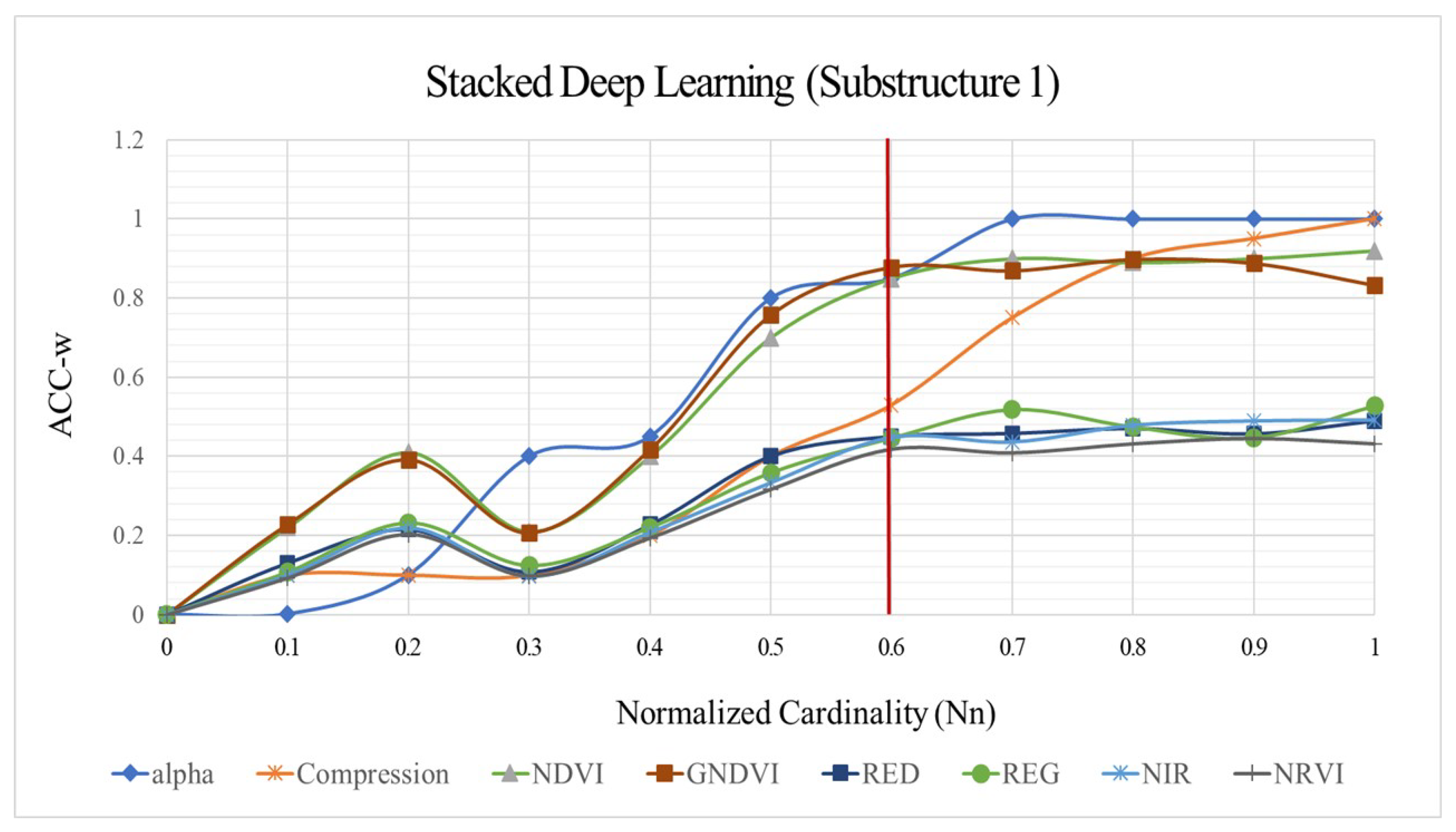
Figure 8 shows the behaviour of Substructure 1 against the identification and labelling of CIs using three MAIS (NIR, REG,RED) and three VIs (NDVI, GNDVI, NRVI). Here, it can be seen how the cardinality was increased when the compression ratios were much higher (first layer). Figure 8 also shows that the Substructure 1 managed to stabilise learning (ACC-w = 0.9933 (NDVI)) when the cardinality reached $60\%$ (six Stacked Layers) for a compression index that was close to $40\%$ (lower computational cost). It is essential to mention that the learning factor ($alpha$) increased as the model became less flexible due to a higher compression of CIs. Overall, Substructure 1 evidenced superior performance levels against the identification and labelling of CIs using the NDVI and GNDVI indices. However, Substructure 1 was able to stabilise learning much more quickly for the NDVI index, as evidenced in Figure 8.

Table 5. Analysis of performance—Substructure 2.

Scenarios	Scenario 3	LG-HDLM	Convolutional DL	Stacked DL	Scenario 1
Hectares (un)	6.9 ha.-1000 un.	6.9 ha.-1000 un.	6.9 ha.-1000 un.	6.9 ha.-1000 un.	6.9 ha.-1000 un.
ELM-ULM-(SLM)	856-143-(1)	858-113-(29)	801-165-(34)	792-130-(78)	744-106-(150)
Distribution	Log-logistic	G.Extrem.V.	Gen.Pareto	G.Extrem.V.	log-logistic
NLogL	1629.45	2054.93	2069.75	2561.85	4206.46
Distribution	Log-normal	Log-logistic	Birnbaum-Saunders	Gen.Pareto	Log-normal
NLogL	1667.76	2069.35	2208.84	2591.12	3488.32
Distribution	Gen.Pareto	Gen.Pareto	Log-logistic	Log-logistic	Birnbaum-Saunders
NLogL	1554.43	2314.51	2314.65	2745.63	3522.90
IOA	1.0000	0.99939	0.99760	0.99067	1.00000
VC	50.78660	148.14748	148.45348	144.14446	148.54747
SK	4.40983	3.46650	3.48849	3.36668	3.45794
KC	30.04629	16.44628	16.77861	15.36103	16.25025
LC (USD)	300.90	6748.40	12,788.25	26,684.02	88,775.88
EL (USD)	5580.69	8726.14	4675.51	4622.98	20,869.56
UL (USD)	6732.67	4409.92	10,470.26	7747.17	4795.67
S-GAP	855	829	767	714	594

shows the results performed by LG-HDLM (Substructure 2) against the risk characterisation defined by the reference scenario (Scenario 1). Performance rates achieved by Substructure 2 show values close to $85\%$ on average ($ELM$:858) against the classification of NDVI-MCOPs by risk category (LW-affectation), which were above the performance rates achieved by the CDLM $80.1\%$ ($ELM$:801) and the SSDLM $79.2\%$ ($ELM$:792), on average, against this same classification. The ALDs showed lean structures with lighter losses due to better risk characterisation (e.g., log-logistic, generalised Pareto, generalised extreme value), and where the projected SL losses given by LG-HDLM were much lower ($\mathrm{SL}:\mathrm{USD}6748.40$) than SL projected losses achieved by CDLM (CDLM ($\mathrm{SL}:\mathrm{USD}\mathrm{12,788.29}$) and SSDLM ($\mathrm{SL}:\mathrm{USD}\mathrm{26,684.02}$) (Figure 9). In this process, the lean distributions were promoted by the goodness of fit against the log-logistic distribution of reference (negative log-likelihood $NlogL=2069.35$), a value much lower than those obtained by the other models when fitting the losses to the log-logistic distribution function representing the activation function for Substructure 2. The above shows the ability of LG-HDLM to identify extended S-$GAPs$ that guarantee environmental and financial sustainability for crops affected by PEs, such as the one suggested by LW for oil-palm crops, ensuring its structural stability against the ALD used for modelling the operational risk.

Table 5 also shows that the models selected by the validation of LG-HDLM were correct, since they had similar behaviours in terms of dimensional stability and structural stability against the ALD of reference, as shown by the $IOA$ indices, which were above $95\%$ on average, and similar values for VC ($148.14748$), SK ($3.46650$), and KC ($16.44628$) indices of the reference scenario (Scenario 1). It is essential to mention that, although LG-HDLM did not show performance values significantly different from those achieved by the validation models, this analysis allowed the demonstration of the fact that the dynamics integrated by LG-HDLM do not distort its ability to characterise the loss structure based on lean ALDs. Regarding stability, Table 5 shows that LG-HDLM reached a similar behaviour concerning the characterisation of losses to the work reported by [20] on the estimation of credibility in the integration of databases for the estimation of operational risk, or with the outcome of [67,68], who offered a broad characterisation of the probability distributions used for the modelling of operational risk (e.g., log-logistic, Weibull, Generalized Pareto).

Table 6. Temporal risk scenarios.

	Scenario 3	Scenario 1	Scenario 2.2	Scenario 2.1	Scenario 2
	Metric	Baseline	Month 4	Month 2	Month 0
Hectares	6.9 (1000)	6.9 (1000)	6.9 (1000)	6.9 (1000)	6.9 (1000)
EL-UL-(SL)	856-143-(1)	744-106-(150)	768-126-(106)	798-144-(58)	840-150-(10)
Distribution	log-logistic	log-logistic	log-logistic	log-logistic	log-logistic
NLogL	1390.20	2314.53	2826.96	3802.20	4206.46
IOA	1.0000	1.00000	0.89820	0.89436	0.089290
VC	50.78660	148.54747	183.55119	212.81653	232.21621
SK	4.40983	3.45794	2.74280	2.47480	2.41750
KC	30.04629	16.25052	12.22450	8.36881	6.09664
ELM	856	858	853	829	792
ULM	143	113	116	136	150
SLM	1	29	30	36	58
EL (USD)	5580.69	8726.14	8122.91	7970.72	7268.19
UL (USD)	6732.67	4409.92	4494.69	5155.76	5506.25
SL (USD)	300	6748.40	6791.23	8193.63	13,554.40
S-GAP	855	829	823	793	733

shows the behaviour exhibited by LG-HDLM against risk characterisation for three temporal risk scenarios describing the evolution of LW in the field for a period of 6 months (Month 0, Month 2, Month 4) before to reference scenario (Scenario 1). Table 6 shows that LG-HDLM performed rates close to $80\%$ on average (Scenario 2-$ELM$:792) against the classification of NDVI-MCOPs by risk category, despite the limitation imposed by the temporal observability of phytosanitary events in stages before to Scenario 1. The probability distributions provided by LG-HDLM for each risk scenario showed slender distributions with light losses and ${NLogL}_{\mathrm{s}}$ that led to a better fit, as the temporal observability concerning the reference scenario was much lower. The latter guarantees the structural stability of LG-HDLM when faced with the characterisation of a risk scenario. It is essential to mention the evolution experienced by ALD distributions, due to the effect of the theoretical development of LW in the field, can be evidenced through dimensional stability characterised by much lower variances and increasingly higher values of skewness (SK) and kurtosis (KC). The suitable performance achieved in general by LG-HDLM was promoted by the novel convolutional mechanism defined by Substructure 2, which integrates an inverse Lagrangian Gaussian dispersion model (I-$LGPTM$) to describe the spatio-temporal evolution of a PE analytically in the field, giving rise to the concept of dynamic vegetation index (forecasting maps). Concerning the characterisation of losses for each of the risk scenarios, LG-HDLM (Substructure 2) yielded probability distributions that evolved towards lower losses, maintaining at all times the loss structure that defines operational risk, which is in line with the work developed by [9,69] on the modelling and evolution of operational risk.

Table 7. IC-Fingerprint fuzzy forecasting analysis.

	EL	UL	SL
	IOA-MG-VG	IOA-MG-VG	IOA-MG-VG	Centroid $\left(xc\right)$	Base $\left(\sigma \right)$
Scenario 2	0.813129	0.850005	0.893388	0.852174	0.080259
Scenario 2.1	0.874696	0.824770	0.830176	0.843214	0.049926
Scenario 2.2	0.896491	0.899339	0.931133	0.908988	0.034642
Scenario 1	0.965450	0.993173	0.996007	0.984877	0.030557
${\sigma }_x$	0.521340	0.456368	0.201632	0.393113	0.319707
${\sigma }_y$	0.482561	0.389754	0.185324	0.352546	0.297237

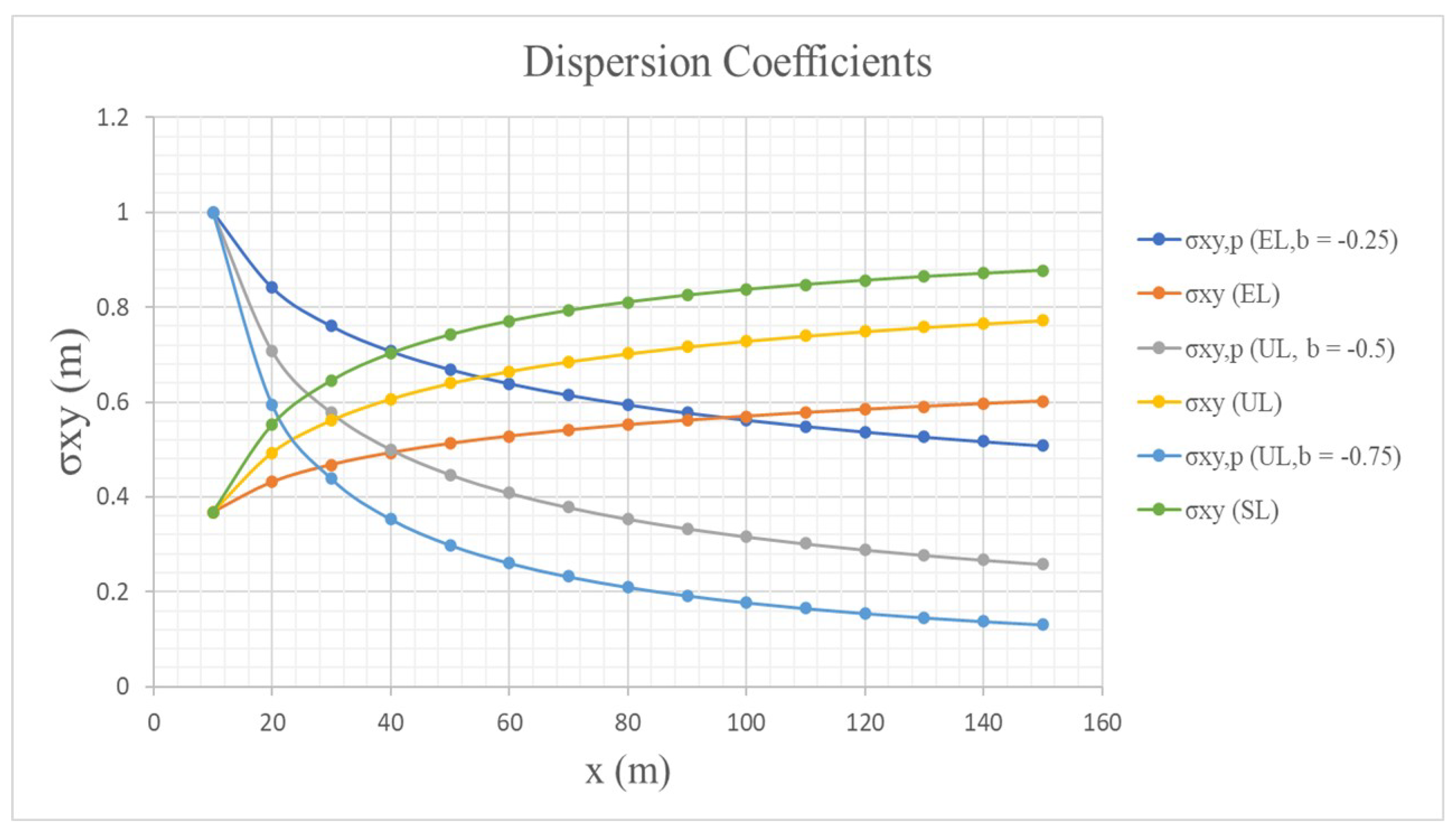
shows the results performed by the fully connected layer (IC fingerprint—Substructure 2) against the classification of NDVI-MCOPs by LW-affectation for each temporal risk scenario. Here, it can be observed that the IC fingerprint indices achieved agreement values close to $80\%$ ($XC$) on average, with variations that were around $5\%$ ($\sigma$) against the NDVI-MCOP convolutional patterns selected from Scenario 1. Once again, the aforementioned shows the ability of LG-HDLM to characterise risk for a temporal scenario (6 months) before the reference scenario (Scenario 1) that shows the natural evolution of a PE in the field. In the context of Lagrangian dispersion models, Table 7 shows that NDVI-MCOP Gaussian functions with wider bases yielded higher values for dispersion parameters (${\sigma }_x$, ${\sigma }_y$), indicating the presence of NDVI-MCOPs in healthy (EL) and apparently healthy (UL) categories; while the Gaussian functions that presented more slender structures showed, on average, the lowest dispersion parameters, which indicates the presence of NDVI-MCOP Gaussian functions affected by LW. The inverse Lagrangian dynamics integrate the convolutional layer, transforming the LG-HDLM into a semi-physical model by adaption, making it ideal for characterising PEs at an early stage, as suggested by LW in the field.

According to Gaussian functions represented by the LW-affectation for MCOPs in the study zone, the spatial structure of the convolutional layer for NDVI index (Substructure 2) can be observed in Figure 10. The figure corroborates that the Gaussian functions with more extended bases indicate the presence of MCOPs in the categories of healthy units (EL) and apparently healthy units (UL), while the Gaussian functions with slender structures indicate the presence of MCOPs affected by LW, which is in-line with the principles of the Lagrangian model presented in Section 3.2. The spatio-temporal evolution of the convolutional layer due to the effect of the semiphysical dispersion dynamics established by the proposed Lagrangian model makes the structure of this layer a forecasting map (dynamic vegetation index) for the characterisation of phytosanitary events at an early stage.

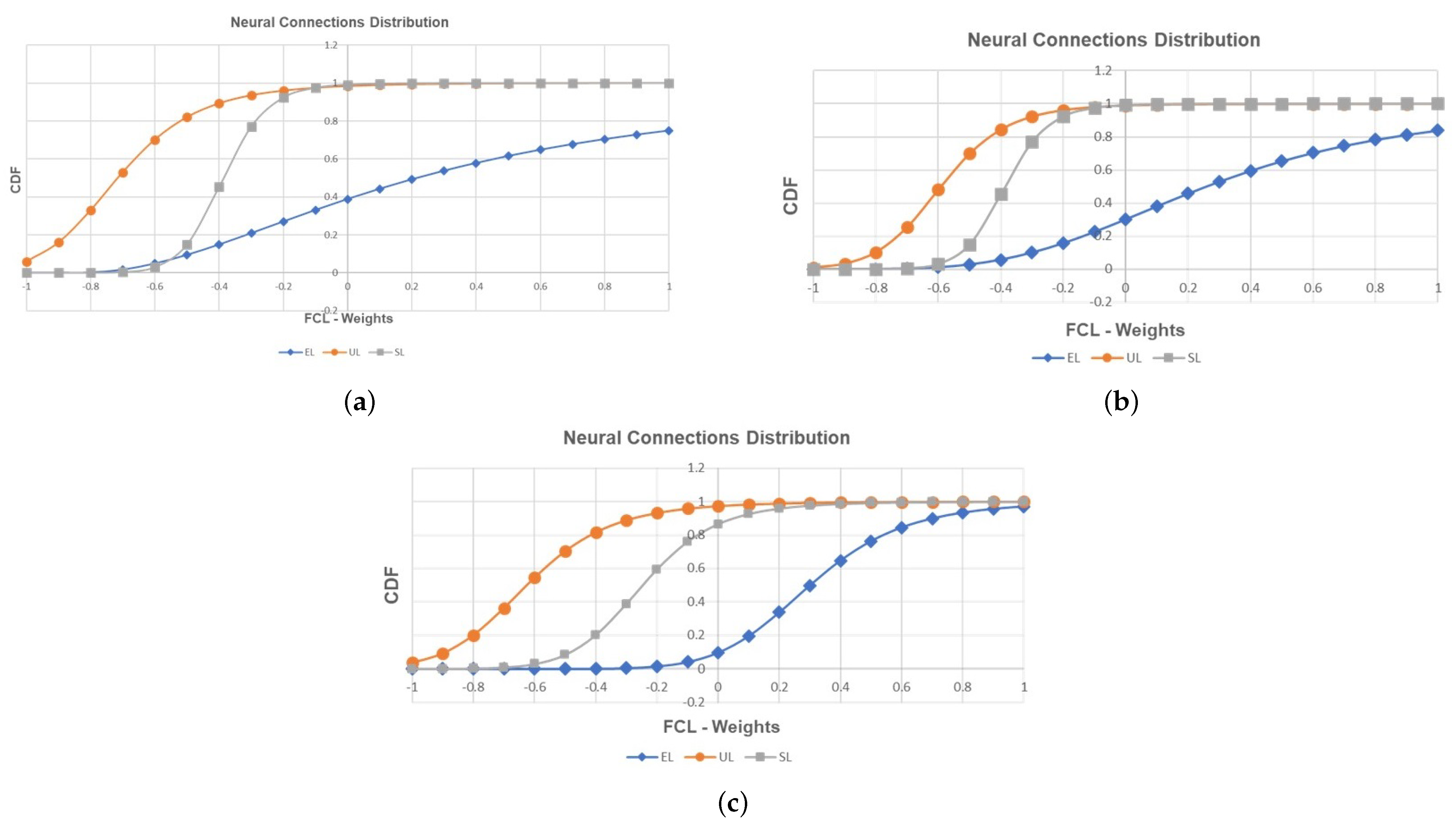
To assess the performance of FCL (fully connected layer) against the risk characterisation, Figure 11 shows the CDFs (cumulative distribution function) for the normalised weights representing the IC fingerprint–FCL relationship by risk category. According to the probability distribution defined by the softmax function (log-logistic distribution Equation (1)), the behaviour of LG-HDLM (Substructure 2) was evaluated based on three parameters: structural factor ($\beta$), stability factor (a), and dimensional factor ($\alpha$) (Equation (17)). Regarding the dimensional factor,

Table 8. Log-logistic structure—normalised weights.

Scenarios	Scenario 2.1			Scenario 2.2			Scenario 2.3
Parameters	EL	UL	SL	EL	UL	SL	EL	UL	SL
a	−0.83	−1.53	−1.38	−0.90	−1.77	−1.38	−0.82	−1.74	$-1.36$
$\alpha$	1.04	0.82	0.99	1.15	1.17	0.99	1.12	0.87	1.02
$\beta$	1.95	6.47	14.45	3.32	11.16	14.45	7.12	8.11	9.32

shows that this factor remained close to unity against the NDVI-MCOPs classification in each of the risk categories defined by a temporal scenario, indicating that the model maintains its stability despite the temporal evolution of a phytosanitary event in the field. Regarding the CDFs for the EL risk category, these showed more extended CDFs, as a result of the increase in the structural factor ($\beta$) due to the effect of the better classification of NDVI-MCOPs. This effect was the opposite for the SL category, which groups the misclassifications of NDVI-MCOPs affected by LW. The dimensional factor ($\alpha$), on the other hand, reached negative values, which shows the tendency of FCL to yield slender distributions in line with the loss structure for ALD. The above clearly shows the ability of LG-HDLM to characterise phytosanitary events in the early stages and to characterise risk parameters ($ELM$-$ULM$-$SLM$) to improve the environmental and financial sustainability (extended S-$GAPs$) of oil-palm crops affected by a PE, as suggested on the LW.

5. Conclusions and Further Studies

LG-HDLM allowed the spatio-temporal characterisation of risks in oil-palm crops affected by a PE, such as LW. The model integrated two deep-learning models into a single structure for this process. A first deep-learning model (Substructure 1: stacked deep-learning structure) for automatic classification of MCOPs from a series of MAIs obtained in the field, and a second deep-learning model (Substructure 2: dynamic convolutional structure) to identify the LW-affectation in MCOPs. To describe the spatio-temporal behaviour of LW in the field, LG-HDLM integrated into Substructure 2 an inverse Lagrangian Gaussian dispersion model. Due to the semiphysical structure by adaptation to phytosanitary risk modelling, LG-HDLM was validated using a novel methodology that integrates financial and environmental metrics according to Basel II agreements and RSPO criteria. The results show the ability of LG-HDLM to identify the evolution of LW for different temporal risk scenarios.

The stability achieved by LG-HDLM against the characterisation of losses generated by LW could be evidenced by the evolution of the ALD structure. In general, LG-HDLM yielded ALDs characteristic of probability distributions with lean structures (structural stability) according to Basel II agreements in operational risk modelling (e.g., log-logistic, log-normal, generalized extreme value), despite the evolution of the ALDs towards lighter loss structures (dimensional stability) as a result of better identification of LW evolution in the field. This stability shows the ability of LG-HDLM to reconstruct a particular structure of losses for different temporary risk scenarios that evolve according to a dispersion Gaussian pattern for LW.

The results yielded by LG-HDLM showed performance rates above $80\%$ on average against loss characterisation for different temporal risk scenarios. This good performance was promoted by similar ALDs structures as shown by the IOA index against losses, which reach values close to $100\%$ with S-GAPs evolving into more extended S-GAPS, despite the temporal observability of identifying early-stage lethal wilt. The stability of these S-GAPs shows the ability of the model to theoretically improve the environmental and financial sustainability of oil-palm crops affected by LW as a result of improved risk management, and to contribute to achieving a balance between development and sustainability in oil-palm crops in the context of the SDA-2030.

Thanks to its adaptive ability and stability in learning against the characterisation of losses for an ALD of reference (Scenario 1), LG-HDLM could be extended to characterise the risk derived from PAEs for other types of crops. In this way, methodologies to identify the dynamic evolution for a particular PAE should be incorporated, converting the convolutional layer (Substructure 2) into a semi-physical dynamic vegetation index (DVI). These DVIs will have the objective of efficient crop management from the phytosanitary point of view, establishing strategies for localised monitoring of PAEs in the field through UAVs. This will lead the model to become a tool for the automatic characterisation of risk parameters in the field as an input for the configuration of index insurances aimed at the differentiated protection of crop units affected by an PAE. It is essential to highlight that index insurances aim to extend S-${GAP}_{\mathrm{s}}$, establishing the proposed model as a natural alternative to achieve a balance between development and sustainability for different crops from risk modelling.

It is essential to highlight that the palm sector in the world will require the certification of around 7,000,000 ha of cultivation and around 31,000,000 tonnes of crude oil under RSPO standards by 2025. This makes it necessary to create technologies that aim to effectively characterise the risks derived from PAEs for this type of crop. It is important to mention that the development of technologies to achieve RSPO certification should include aspects related to: the optimisation and efficiency of productivity; the protection, conservation and improvement of the environment; and sustainable livelihoods, poverty reduction and social inclusion, in line with the planet’s sustainable development goals (SDGs). In this sense, LG-HDLM aims to improve production efficiency by integrating financial criteria to protect, conserve and improve the environment.

For effective risk management in crops, the authors propose the creation of an augmented intelligence platform for the real-time monitoring of PAEs. This platform will integrate into a single structure a series of DVIs using hyperspectral technologies to expand the reflectance spectrum in the characterisation of crop units affected by a particular PAE; and IOT-IOB networks (Internet of Things and Beings) using different communication technologies (e.g., LORA, Zigbee) with the objective of monitoring in the field the balance between climate, host (unit) and vectors. Accordingly, this platform will result in a series of forecasting maps to identify emerging risks, enabling the management of risk of PEs at an early stage. The above will bring about a natural reduction in insecticides and fertilisers and, consequently, a reduction in the emission of GHGs from agricultural activities.

References

1. Chopra, R.; Magazzino, C.; Shah, M.I.; Sharma, G.D.; Rao, A.; Shahzad, U. The role of renewable energy and natural resources for sustainable agriculture in ASEAN countries: Do carbon emissions and deforestation affect agriculture productivity? Resour. Policy 2022, 76, 102578. [Google Scholar] [CrossRef]
2. Maluin, F.N.; Hussein, M.Z.; Idris, A.S. An Overview of the Oil Palm Industry: Challenges and Some Emerging Opportunities for Nanotechnology Development. Agronomy 2020, 10, 356. [Google Scholar] [CrossRef] [Green Version]
3. Lai, O.; Tan, C.; Akoh, C. Palm Oil: Production, Processing, Characterization, and Uses; Elsevier Science: Amsterdam, The Netherlands, 2015. [Google Scholar]
4. Corley, H.; Tinker, P. The Oil Palm; Wiley Online Library: Hoboken, NJ, USA, 2015. [Google Scholar] [CrossRef]
5. Khatun, R.; Reza, M.; Moniruzzaman, M.; Yaakob, Z. Sustainable oil palm industry: The possibilities. Renew. Sustain. Energy Rev. 2017, 76, 608–619. [Google Scholar] [CrossRef]
6. Castanheira, É.G.; Acevedo, H.; Freire, F. Greenhouse gas intensity of palm oil produced in colombia addressing alternative land use change and fertilization scenarios. Appl. Energy 2014, 114, 958–967. [Google Scholar] [CrossRef]
7. Mosquera, M.; Valderrama, M.; Ruiz, E.; Lopez, D.; Castro, L. Costos de producción para el fruto de palma de aceite y el aceite de palma en 2015: Estimación en un grupo de productores colombianos. Palmas 2017, 38, 10–26. [Google Scholar]
8. Peña, A.; Bonet, I.; Lochmuller, C.; Chiclana, F.; Góngora, M. Flexible inverse adaptive fuzzy inference model to identify the evolution of operational value at risk for improving operational risk management. Appl. Soft Comput. 2018, 65, 614–631. [Google Scholar] [CrossRef] [Green Version]
9. Peña, A.; Bonet, I.; Lochmuller, C.; Patiño, H.A.; Chiclana, F.; Góngora, M. A fuzzy credibility model to estimate the Operational Value at Risk using internal and external data of risk events. Knowl.-Based Syst. 2018, 159, 98–109. [Google Scholar] [CrossRef] [Green Version]
10. Rspo Roundtable for Sustainability Palm Poil. Rspo Principles and Criteria for the Production of Sustainable Palm Oil; RSPO Roundtable for Sustainability Palm Oil: Geneva, Switzerland, 2018. [Google Scholar]
11. Diaz, J. Estudio de índices de Vegetación a Partir de Imágenes Aéreas Tomadas Desde Uas/Rpas y Aplicaciones de éstos a la Agricultura de Precisión. Ph.D. Thesis, Universidad Complutense de Madrid, Madrid, Spain, 2015. [Google Scholar]
12. P, A.P.; Hernández, J.A.; Toro, V.M. Computational evolutionary inverse lagrangian puff model. Environ. Model. Softw. 2010, 25, 1890–1893. [Google Scholar] [CrossRef]
13. Sadi, M.; Mahani, A. Accelerating Deep Convolutional Neural Network base on stochastic computing. Integration 2021, 76, 113–121. [Google Scholar] [CrossRef]
14. Mohammed, M.; Mwambi, H.; Mboya, I.B.; Elbashir, M.K.; Omolo, B. A stacking ensemble deep learning approach to cancer type classification based on TCGA data. Sci. Rep. 2021, 11, 15626. [Google Scholar] [CrossRef]
15. Nevruz, E.; Yildirak, K. Spatiotemporal interpolation through an extension of differential evolution algorithm for agricultural insurance claims. J. Comput. Appl. Math. 2019, 352, 278–292. [Google Scholar] [CrossRef]
16. Fitrianto, A.; Darmawan, A.; Tokimatsu, K.; Sufwandika, M. Estimating the age of oil palm trees using remote sensing technique. In Proceedings of the IOP Conference Series: Earth and Environmental Science, Banda Aceh, Indonesia, 26–27 September 2018; IOP Publishing: Bristol, UK, 2018; Volume 148, p. 012020. [Google Scholar] [CrossRef] [Green Version]
17. Baseca, C.; Sendra, S.; Lloret, J.; Tomas, J. A smart decision system for digital farming. Agronomy 2019, 9, 216. [Google Scholar] [CrossRef] [Green Version]
18. Shamshiri, R.R.; Hameed, I.A.; Balasundram, S.K.; Ahmad, D.; Weltzien, C.; Yamin, M. Fundamental Research on Unmanned Aerial Vehicles to Support Precision Agriculture in Oil Palm Plantations. In Agricultural Robots-Fundamentals and Applications; IntechOpen: London, UK, 2019; Chapter 6; pp. 255–265. [Google Scholar] [CrossRef] [Green Version]
19. Popovic, T.; Nedeljko, L.; Pesic, A.; Zecevic, Z.; Krstajic, B.; Djukanovic, S. Architecting an iot-enabled platform for precision agriculture and ecological monitoring: A case study. Comput. Electron. Agric. 2017, 140, 255–265. [Google Scholar] [CrossRef]
20. Pena, A.; Patino, A.; Chiclana, F.; Caraffini, F.; Gongora, M.; Gonzalez-Ruiz, J.D.; Duque-Grisales, E. Fuzzy convolutional deep-learning model to estimate the operational risk capital using multi-source risk events. Appl. Soft Comput. 2021, 107, 107381. [Google Scholar] [CrossRef]
21. Wang, Y.M.; Ostendorf, B.; Gautam, D.; Habili, N.; Pagay, V. Plant Viral Disease Detection: From Molecular Diagnosis to Optical Sensing Technology;A Multidisciplinary Review. Remote Sens. 2022, 14, 1542. [Google Scholar] [CrossRef]
22. Xue, J.; Su, B. Significant remote sensing vegetation indices: A review of developments and applications. J. Sensors 2017, 1353691. [Google Scholar] [CrossRef] [Green Version]
23. Paula Ramos, P.; Solarte, E.; Valdés, C.; Sanz, J.; Gómez, E. Características espectrales de la luz reflejada por frutos de café (coffea arabica). Rev. Soc. Colomb. Física 2018, 38, 822–825. [Google Scholar]
24. Raza, S.e.A.; Prince, G.; Clarkson, J.P.; Rajpoot, N.M. Automatic Detection of Diseased Tomato Plants Using Thermal and Stereo Visible Light Images. PLoS ONE 2015, 10, 1–20. [Google Scholar] [CrossRef]
25. Johansen, K.; Duan, Q.; Tu, Y.H.; Searle, C.; Wu, D.; Phinn, S.; Robson, A.; McCabe, M.F. Mapping the condition of macadamia tree crops using multi-spectral UAV and WorldView-3 imagery. ISPRS J. Photogramm. Remote Sens. 2020, 165, 28–40. [Google Scholar] [CrossRef]
26. Candiago, S.; Remondino, F.; De Giglio, M.; Dubbini, M.; Gattelli, M. Evaluating Multispectral Images and Vegetation Indices for Precision Farming Applications from UAV Images. Remote Sens. 2015, 7, 4026–4047. [Google Scholar] [CrossRef] [Green Version]
27. Peña, P.A.; Patiño, P.A.; Velásquez, V.J.; Góngora, M. Inteligent system to identify oil palm crop units from multispectral aerial images: Identification of multispectral patterns. In Proceedings of the 2017 12th Iberian Conference on Information Systems and Technologies (CISTI), Lisbon, Portugal, 21–24 June 2017; pp. 1–7. [Google Scholar] [CrossRef]
28. Pena, A.; Patino, A.; Bonet, I.; Gongora, M. Fuzzy spatial maps to identify oil palm units: Spatial fuzzy maps. In Proceedings of the 2018 13th Iberian Conference on Information Systems and Technologies (CISTI), Caceres, Spain, 13–16 June 2018; pp. 1–6. [Google Scholar] [CrossRef]
29. Khai Loong, C.; Kanniah, K.; Pohl, C.; Tan, K. A review of remote sensing applications for oil palm studies. Geo-Spat. Inf. Sci. 2017, 20, 184–200. [Google Scholar] [CrossRef] [Green Version]
30. Bhandari, A.; Kumar, A.; Singh, G. Feature extraction using normalized difference vegetation index (ndvi): A case study of jabalpur city. Procedia Technol. 2012, 6, 612–621. [Google Scholar] [CrossRef] [Green Version]
31. Torres-Sánchez, J.; López-Granados, F.; De Castro, A.; Peña-Barragán, J.M. Configuration and Specifications of an Unmanned Aerial Vehicle (UAV) for Early Site Specific Weed Management. PLoS ONE 2013, 8, e58210. [Google Scholar] [CrossRef] [Green Version]
32. Mu, X.; Song, W.; Gao, Z.; McVicar, T.R.; Donohue, R.J.; Yan, G. Fractional vegetation cover estimation by using multi-angle vegetation index. Remote Sens. Environ. 2018, 216, 44–56. [Google Scholar] [CrossRef]
33. Mohanty, S.P.; Hughes, D.P.; Salathé, M. Using Deep Learning for Image-Based Plant Disease Detection. Front. Plant Sci. 2016, 7, 1419. [Google Scholar] [CrossRef] [Green Version]
34. Sladojevic, S.; Arsenovic, M.; Anderla, A.; Culibrk, D. Stefanovic, D. Deep Neural Networks Based Recognition of Plant Diseases by Leaf Image Classification Computational Intelligence and Neuroscience. Comput. Intell. Neurosci. 2016, 2016, 11. [Google Scholar] [CrossRef] [Green Version]
35. Lu, Y.; Yi, S.; Zeng, N.; Liu, Y.; Zhang, Y. Identification of rice diseases using deep convolutional neural networks. Neurocomputing 2017, 267, 378–384. [Google Scholar] [CrossRef]
36. Langford, Z.L.; Kumar, J.; Hoffman, F.M. Convolutional Neural Network Approach for Mapping Arctic Vegetation Using Multi-Sensor Remote Sensing Fusion. In Proceedings of the 2017 IEEE International Conference on Data Mining Workshops (ICDMW), New Orleans, LA, USA, 18–21 November 2017; pp. 322–331. [Google Scholar] [CrossRef]
37. Paoletti, M.; Haut, J.; Plaza, J.; Plaza, A. A new deep convolutional neural network for fast hyperspectral image classification. ISPRS J. Photogramm. Remote Sens. 2018, 145, 120–147. [Google Scholar] [CrossRef]
38. Park, H.G.; Yun, J.P.; Kim, M.Y.; Jeong, S.H. Multichannel Object Detection for Detecting Suspected Trees With Pine Wilt Disease Using Multispectral Drone Imagery. IEEE J. Sel. Top. Appl. Earth Obs. Remote Sens. 2021, 14, 8350–8358. [Google Scholar] [CrossRef]
39. Romero, M.; Luo, Y.; Su, B.; Fuentes, S. Vineyard water status estimation using multispectral imagery from an UAV platform and machine learning algorithms for irrigation scheduling management. Comput. Electron. Agric. 2018, 147, 109–117. [Google Scholar] [CrossRef]
40. Torres, A.; Camacho, J.; Torres, J.; Cruz-Roa, A. Análisis preliminar de detección de patologías en cultivos de palma aceitera usando Redes Neuronales Convolucionales. In Proceedings of the III Congreso Internacional de Ciencias Básicas e Ingeniería—CICI 2020, Villavicencio, Colombia, 11–13 August 2020. [Google Scholar]
41. Bonet, I.; Peña, A.; Lochmuller, C.; Patiño, H.A.; Chiclana, F.; Góngora, M. Applying fuzzy scenarios for the measurement of operational risk. Appl. Soft Comput. 2021, 112, 107785. [Google Scholar] [CrossRef]
42. Ghaffarian, S.; van der Voort, M.; Valente, J.; Tekinerdogan, B.; de Mey, Y. Machine learning-based farm risk management: A systematic mapping review. Comput. Electron. Agric. 2022, 192, 106631. [Google Scholar] [CrossRef]
43. Peña, A.; Bonet, I.; Lochmuller, C.; Chiclana, F.; Góngora, M. An integrated inverse adaptive neural fuzzy system with Monte-Carlo sampling method for operational risk management. Expert Syst. Appl. 2018, 98, 11–26. [Google Scholar] [CrossRef]
44. Herbold, J. Herbold, J. Crop insurance in developing economies: The insurers’ and reinsurers’ perspective. Int. J. Rural Dev. 2010, 4, 14–18. [Google Scholar]
45. Van-Gelder, J.; Sari, A.; Pacheco, P. Managing Palm Oil Risks: A Brief for Financiers; Roundtable for sustainable palm oil rspo; Profundo; Center for International Forestry Research: Bogor, Indonesia, 2017. [Google Scholar]
46. Kath, J.; Mushtaq, S.; Henry, R.; Adeyinka, A.; Stone, R. Index insurance benefits agricultural producers exposed to excessive rainfall risk. Weather Clim. Extrem. 2018, 22, 1–9. [Google Scholar] [CrossRef]
47. Shirsath, P.; Vyas, S.; Aggarwal, P.; Rao, K.N. Designing weather index insurance of crops for the increased satisfaction of farmers, industry and the government. Clim. Risk Manag. 2019, 25, 100189. [Google Scholar] [CrossRef]
48. Magazzino, C.; Mele, M.; Santeramo, F.G. Using an Artificial Neural Networks Experiment to Assess the Links among Financial Development and Growth in Agriculture. Sustainability 2021, 13, 2828. [Google Scholar] [CrossRef]
49. Trenca, I.; Pece, A.M.; Mihuţ, I.S. The Assessment of Market Risk in the Context of the Current Financial Crisis. Procedia Econ. Financ. 2015, 32, 1391–1406. [Google Scholar] [CrossRef] [Green Version]
50. Basel Committee on Banking Supervision. High-Level Summary of Basel III Reforms; Bank for International Settlements: Basel, Switzerland, 2017. [Google Scholar]
51. Specht, D.F. Probabilistic neural networks. Neural Netw. 1990, 3, 109–118. [Google Scholar] [CrossRef]
52. Hornik, K.; Grün, B. On conjugate families and Jeffreys priors for von Mises–Fisher distributions. J. Stat. Plan. Inference 2013, 143, 992–999. [Google Scholar] [CrossRef] [Green Version]
53. UNIPALMA de los Llanos, S.A. Guia Técnica-Polinización Asistida en Palma de Aceite; UNIPALMA de Los LLanos S.A.: Bogotá, Colombia, 2018. [Google Scholar]
54. DJI-Industries, Phantom 3 Professional. 2018. Available online: https://www.dji.com/phantom-3-pro/info (accessed on 24 April 2022).
55. Parrot, Parrot Sequoia-Multispectral Camera. 2018. Available online: https://www.parrot.com/uk/shop/accessories-spare-parts/other-drones/sequoia (accessed on 24 April 2022).
56. Woittiez, L.S.; van Wijk, M.T.; Slingerland, M.; van Noordwijk, M.; Giller, K.E. Yield gaps in oil palm: A quantitative review of contributing factors. Eur. J. Agron. 2017, 83, 57–77. [Google Scholar] [CrossRef]
57. Magazzino, C.; Mele, M.; Sarkodie, S.A. The nexus between COVID-19 deaths, air pollution and economic growth in New York state: Evidence from Deep Machine Learning. J. Environ. Manag. 2021, 286, 112241. [Google Scholar] [CrossRef] [PubMed]
58. Nanni, A.; Tinarelli, G.; Solisio, C.; Pozzi, C. Comparison between Puff and Lagrangian Particle Dispersion Models at a Complex and Coastal Site. Atmosphere 2022, 13, 508. [Google Scholar] [CrossRef]
59. Arango, M.; Ospina, C.; Martínez, G. Uso de herramientas epidemiológicas para establecer el manejo integrado de la Marchitez letal de la palma de aceite. Palmas 2011, 32, 17–27. [Google Scholar]
60. Liu, G.; Bao, H.; Han, B. A Stacked Autoencoder-Based Deep Neural Network for Achieving Gearbox Fault Diagnosis. Math. Probl. Eng. 2018, 2018, 1–10. [Google Scholar] [CrossRef] [Green Version]
61. Peña, A.; Bonet, I.; Manzur, D.; Góngora, M.; Caraffini, F. Validation of convolutional layers in deep learning models to identify patterns in multispectral images. In Proceedings of the 2019 14th Iberian Conference on Information Systems and Technologies (CISTI), Coimbra, Portugal, 19–22 June 2019; pp. 1–6. [Google Scholar] [CrossRef]
62. Charte, D.; Charte, F.; Herrera, F. Reducing Data Complexity using Autoencoders with Class-informed Loss Functions. IEEE Trans. Pattern Anal. Mach. Intell. 2021. [Google Scholar] [CrossRef]
63. Gao, B.; Pavel, L. On the Properties of the Softmax Function with Application in Game Theory and Reinforcement Learning. arXiv 2017, arXiv:1704.00805. [Google Scholar]
64. Park, O.H.; Seok, M.G. Selection of an appropriate model to predict plume dispersion in coastal areas. Atmos. Environ. 2007, 41, 6095–6101. [Google Scholar] [CrossRef]
65. Izzuddin, M.; Nisfariza, M.N.; Ezzati, B.; Idris, A.S.; Steven, M.D.; Boyd, D. Analysis of airborne hyperspectral image using vegetation indices, red edge position and continuum removal for detection of Ganoderma disease in oil palm. J. Oil Palm Res. 2018, 30, 416–428. [Google Scholar]
66. Srestasathiern, P.; Rakwatin, P. Oil Palm Tree Detection with High Resolution Multi-Spectral Satellite Imagery. Remote Sens. 2014, 6, 9749–9774. [Google Scholar] [CrossRef] [Green Version]
67. Mora, A. Cuantificación del Riesgo Operativo en Entidades Financieras en Colombia. Cuad. Adm. 2010, 23, 185–211. [Google Scholar]
68. Jantsch, L.; Solana-González, P.; Vanti, A.A. Management of Corporate Risk in Financial Institutions: An Evidence of Loss Events Derived from Operational Risk. Rev. Espac. 2019, 40, 21–30. Available online: https://revistaespacios.com/a19v40n06/a19v40n06p21.pdf (accessed on 24 April 2022).
69. Bolance, C.; Guillén, M.; Gustafsson, J.; Nielsen, J. Quantitative Operational Risk Models, 1st ed.; Chapman and Hall: London, UK, 2012. [Google Scholar] [CrossRef]
Figure 1. Aggregate loss distribution.
Sustainability 14 06668 g001
Figure 2. Red edge multispectral band (Height: 10 m).
Sustainability 14 06668 g002
Figure 3. Normalised difference vegetation index (MCOP patterns).
Sustainability 14 06668 g003
Figure 4. Lethal wilt dispersion coefficients.
Sustainability 14 06668 g004
Figure 5. NDVI oil-palm crops affected by a phytosanitary event ( a = 1 ) (a) healthy palm (EL, b= 0.25 ), (b) apparently healthy palm (UL, b= 0.5 ), (c) palm affected by LW (SL, b= 0.75 ).
Sustainability 14 06668 g005
Figure 6. LW pattern dispersion in the field.
Sustainability 14 06668 g006
Figure 7. NDVI-CIs classified by Substructure 1: (a) NDVI-MCOP (Height: 10 m), (b) NDVI non-MCOP, (c) Forrest NDVI non-MCOP.
Sustainability 14 06668 g007
Figure 8. Stacked deep-learning configuration (Substructure 1).
Sustainability 14 06668 g008
Figure 9. Aggregate Loss Distributions ALD-Validation Process.
Sustainability 14 06668 g009
Figure 10. Convolutional forecasting map.
Sustainability 14 06668 g010
Figure 11. Neural connections between the IC fingerprint and the FCL layer. (a) Scenario 2.1; (b) Scenario 2.2; (c) Scenario 2.3.
Sustainability 14 06668 g011