Article

Influence of Source Apportionment of PAHs Occurrence in Aquatic Suspended Particulate Matter at a Typical Post-Industrial City: A Case Study of Freiberger Mulde River

1
Department of Ecology and Institute of Hydrobiology, Jinan University, Guangzhou 510632, China
2
Institute of Urban and Industrial Water Management, Technische Universität Dresden, 01062 Dresden, Germany
3
Safety, Environment and Technology Supervision Research Institute, PetroChina Southwest Oil and Gas Field Company, Chengdu 610041, China
4
State Key Laboratory of Desert and Oasis Ecology, Xinjiang Institute of Ecology and Geography, Chinese Academy of Sciences, Urumqi 830011, China
5
Yangtze Institute for Conservation and Development, State Key Laboratory of Hydrology-Water Resources and Hydraulic Engineering, Hohai University, Nanjing 210098, China
*
Author to whom correspondence should be addressed.
Sustainability 2022, 14(11), 6646; https://doi.org/10.3390/su14116646
Submission received: 21 April 2022 / Revised: 26 May 2022 / Accepted: 26 May 2022 / Published: 29 May 2022
(This article belongs to the Topic Climate Change and Environmental Sustainability)

Abstract

:
Polycyclic aromatic hydrocarbons (PAHs) have received extensive attention because of their widespread presence in various environmental media and their high environmental toxicity. Thus, figuring out the long-term variances of their occurrence and driving force in the environment is helpful for environmental pollution control. This study investigates the concentration levels, spatial variance, and source apportionment of PAHs in suspended particulate matter of Freiberger Mulde river, Germany. Results show that the concentrations of the 16 priority PAHs suggested by USEPA (Σ16PAHs) were in the range of 707.0–17,243.0 μg kg−1 with a mean value of 5258.0 ± 2569.2 μg kg−1 from 2002 to 2016. The relatively high average concentrations of Σ16PAHs were found in the midstream and upstream stations of the given river (7297.5 and 6096.9 μg kg−1 in Halsbrucke and Hilbersdorf, respectively). In addition, the annual average concentration of Σ16PAHs showed an obvious decreasing pattern with time. Positive Matrix Factorization (PMF) receptor model identified three potential sources: coke ovens (7.6–23.0%), vehicle emissions (35.9–47.7%), and coal and wood combustion (34.5–47.3%). The source intensity variation and wavelet coherence analysis indicated that the use of clean energy played a key role in reducing PAHs pollution levels in suspended sediments. The risk assessment of ecosystem and human health suggested that the Σ16PAHs in the given area posed a non-negligible threat to aquatic organisms and humans. The data provided herein could assist the subsequent management of PAHs in the aquatic environment.

1. Introduction

Polycyclic aromatic hydrocarbons (PAHs), which consist of a group of hydrocarbons composed of two or more linear, angular, or clustered benzene rings, have received high attention because they are abundant in the ecological environment and their high carcinogenicity, genotoxicity teratogenicity, bioaccumulation [1,2,3]. PAHs enter the environment through various pathways, which might pose a serious threat to environmental organisms. As many as 200 forms of PAHs and their metabolites have been identified, among which Σ16PAHs were regarded as the main contaminants [4,5]. Therefore, an in-depth investigation of the occurrence of PAHs in the environment and its associated driving forces is essential.
Regarding the environmental behaviors, PAHs widely exist in a variety of environmental media, such as the atmosphere [6,7,8], water [1,7,9], sediments [10,11,12], soil [13,14,15], and road dust [16,17,18,19]. Research has proven that the aquatic suspended sediment was an important sink and transport medium of PAHs discharged into the environment [1,20,21]. Therefore, investigating concentration levels, spatial distribution, and source apportionments of PAHs in the water system is helpful to mitigate PAH in the aquatic environment.
Changes in the source dynamics of PAHs often lead to spatiotemporal differences in their concentrations and compositional characteristics in the environment. Quantitatively analyzing the changes in the source contribution of PAHs in the environment could help to investigate the impact of human activities on the occurrence of PAHs in the environment. There have been many studies on the source identification of PAHs in river suspended sediments [22,23,24,25]. However, quantitative analysis studies on long-term changes in the source driving forces of PAHs in suspended sediments are still lacking.
In terms of source apportionment, the receptor model has been a commonly used source identification method, which identifies the main factors affecting the dataset by extracting the key characteristic information in the environmental dataset, such as principal component analysis (PCA) [16,26,27], chemical mass balance (CMB) [26,28,29], UNMIX [13,16,27], and positive matrix factorization (PMF) [16,30,31]. The PMF model is the most widely used receptor model in recent years [14,32]. It imposes non-negative constraints on the source profile matrix and the source contribution matrix to improve the physical meaning of the model solution [30,33]. In addition, PMF affords users the ability to process input data individually, thus helping reduce the possible adverse effects of data anomalies caused by sampling, experimentation, or other processes on the source apportionment results [34,35,36]. Compared with other receptor models, the PMF model has higher accuracy and stability, and it can calculate more complete and detailed source apportionment results [12,37,38]. Therefore, the PMF model was employed in this study to conduct the quantitative source identification of PAHs in suspended particulate matter in the aquatic environment.
Accordingly, to characterize the occurrence of PAHs in the aquatic environment, a long-term variation and source shift were investigated. The detailed focuses were to (1) firstly evaluate the concentration level, the spatiotemporal distribution of PAH in the suspended particulate matter; (2) figure out the potential sources and their driving force during the long-term period; and (3) assess the ecological risk and possible human hazards posed by PAHs in the given area.

2. Materials and Methods

2.1. Study Area

The Mulde river (consisting of the Freiberger Mulde, the Zwickauer Mulde, and the Vereinigte Mulde) is one of the most diverse ecosystems in the Saxony state, Germany. In the past, the Mulde river basin has received widespread attention due to its thriving mining activities [39,40,41]. The Freiberger Mulde river originates near Moldova on the Erzgebirge ridge in the Czech Republic and flows north to Freiberg in Saxony, Germany. The Czech Republic and the state of Saxony experienced relatively rapid urbanization and significant economic growth during 2002–2016, which might lead to more serious PAHs pollution in the river.
The locations of PAH measurement stations in the Freiberger Mulde river are shown in Figure 1. Sampling data for the suspended particulate matters were obtained at 6 stations: Katzenstein (upstream), Hilbersdorf (midstream), Halsbrucke (midstream), Siebenlehn (midstream), Dobeln (midstream), and Erlln (downstream). Suspended particulate matter samples were obtained mainly using centrifugation or filtration of residues from special sedimentation tanks (mostly monthly mixed samples) at the measuring stations. In this study, 16 PAHs, namely naphthalene (NAP), acenaphthene (ACY), acenaphthene (ACE), fluorene (FLU), phenanthrene (PHE), anthracene (ANT), fluoranthene (FLUH), pyrene (PYR), benzo[a]an-thracene (BaA), chrysene (CHR), benzo[b]fluoranthene (BbF), benzo[k]fluoranthene (BkF), benzo[a]pyrene (BaP), dibenzo[a,h]anthracene (DBA), indeno [1,2,3-cd]pyrene (IDP) and benzo[g,h,i]perylene (BgP), were analyzed. The detailed information on the sampling collection and analysis is provided in Section S1 of Supplementary Materials.

2.2. PMF Receptor Model

PMF is a multivariate analysis model that solves the problem in the weighted least squares sense with non-negative constraints [35]. The data matrix provided by the user would be divided into factor contribution matrix G, factor profiles matrix F, and residual matrix E. It supposes X as the initial data set:
X = G F + E
The elements e i j of matrix E could be written as:
e i j = x i j ( k = 1 ) p g i k f k j
where e i j is residual content for the jth pollutant determined in the ith sample. x i j is the concentration of jth pollutant determined in the ith sample, g i k is the relative contribution of factor k to sample i, and f k j is the concentration of jth pollutant in factor profile k.
The PMF model aims to reduce the residual matrix Q to a minimum. The function Q with f k j   0 , g i k 0 is expressed as:
Q = i = 1 n j = 1 m ( x i j k = 1 p g i k f k j u i j ) 2 = i = 1 n j = 1 m ( e i j u i j ) 2
where u i j is the data uncertainty. The missing values in the data matrix are suggested to replace by species median values.

2.3. Wavelet Analysis

Wavelet analysis has been widely used to decompose time series to characterize their significant local power changes [3,42,43]. Wavelet analysis divides the variations in time series into time scales and time locations, which helps researchers to further analyze local changes in time series [44]. A detailed introduction to the wavelet analysis method is provided in Section S2 of Supplementary Materials. Wavelet coherence (WTC) is used to analyze the degree of local correlation of the sequence. In this study, wavelet coherence was used to analyze the potential correlations of temporal variations between PAHs concentrations in suspended sediments and the anthropogenic emissions-related indicators (e.g., fuel, vehicle emissions, etc.). The WTC coefficient is calculated by the following formula [45]:
R 2 ( a ,   b ) = S ( a 1 | W x y ( a ,   b ) | 2 ) S ( a 1 | W x ( a ,   b ) | 2 ) · S ( a 1 | W y ( a ,   b ) | 2 )
where 0 < R2(a, b) < 1 and S is the smoothing operator.

2.4. Ecological Risk Assessment

The sediment ecological toxicity screening guideline for ERL and the U.S. National Oceanic and Atmospheric Administration’s effect range median (ERM) values were used to determine the possible biological effects of PAHs in aquatic sediment [46]. The hazard quotient (HQ) for different PAHs was determined as the ratio between the concentration of individual PAHs (μg kg−1) and the ERM [47,48]. Therefore, the values of HQ and MHQ were obtained for the total PAHs:
H Q i = C i / E R M i
M H Q i = H Q i / n
where C i is the content of species i (μg kg−1), E R M i is the ERM value of species i, and n is the number of PAHs. For example, if the value of MHQ was less than 0.11, indicating that there was a 9% probability of being toxic to benthic fauna, while the value within the range of 0.11–0.5 indicates a probability of 21%; the value between 0.51 and 1.5 indicates a probability of 49%, and the higher value represents a probability of 76% [49].

2.5. Carcinogenic Risk Assessment

The potential carcinogenic risk was determined based on the value of toxic benzo[a]pyrene equivalent (TEQ). To transform the concentration and estimation of benzo[a]pyrene equivalent doses, the TEFs used in this study are provided in Table S2 [50,51,52]. PAHs species i was calculated as follows:
B a P i d o s e i = T E F i × C i
where C i is the content of species i (μg kg−1), and T E F i is the toxic factor of species i. The TEF values of individual PAHs are listed in Table S2. The total TEQ can be calculated by:
T E Q = i B a P i d o s e i

3. Results and Discussion

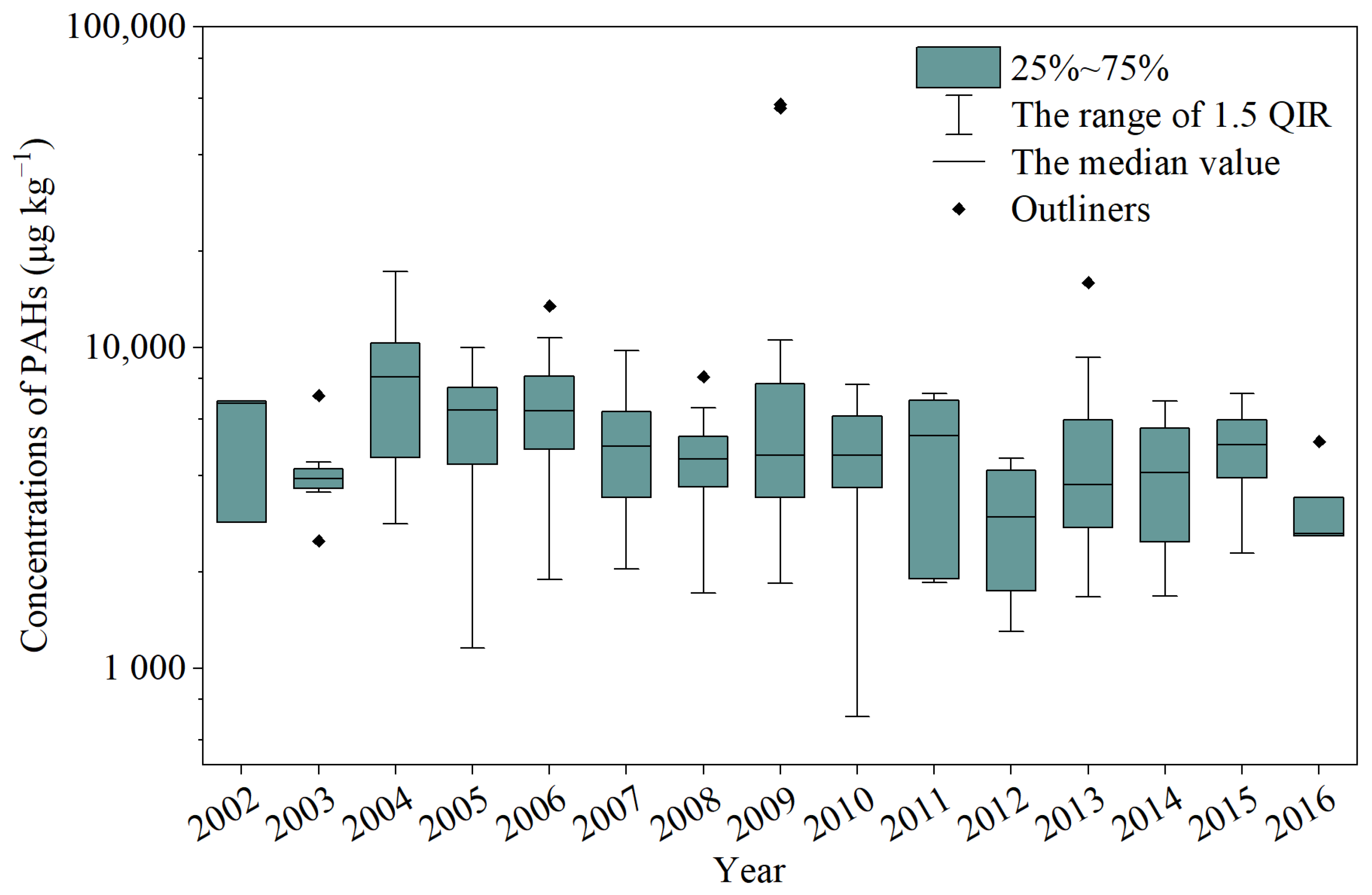
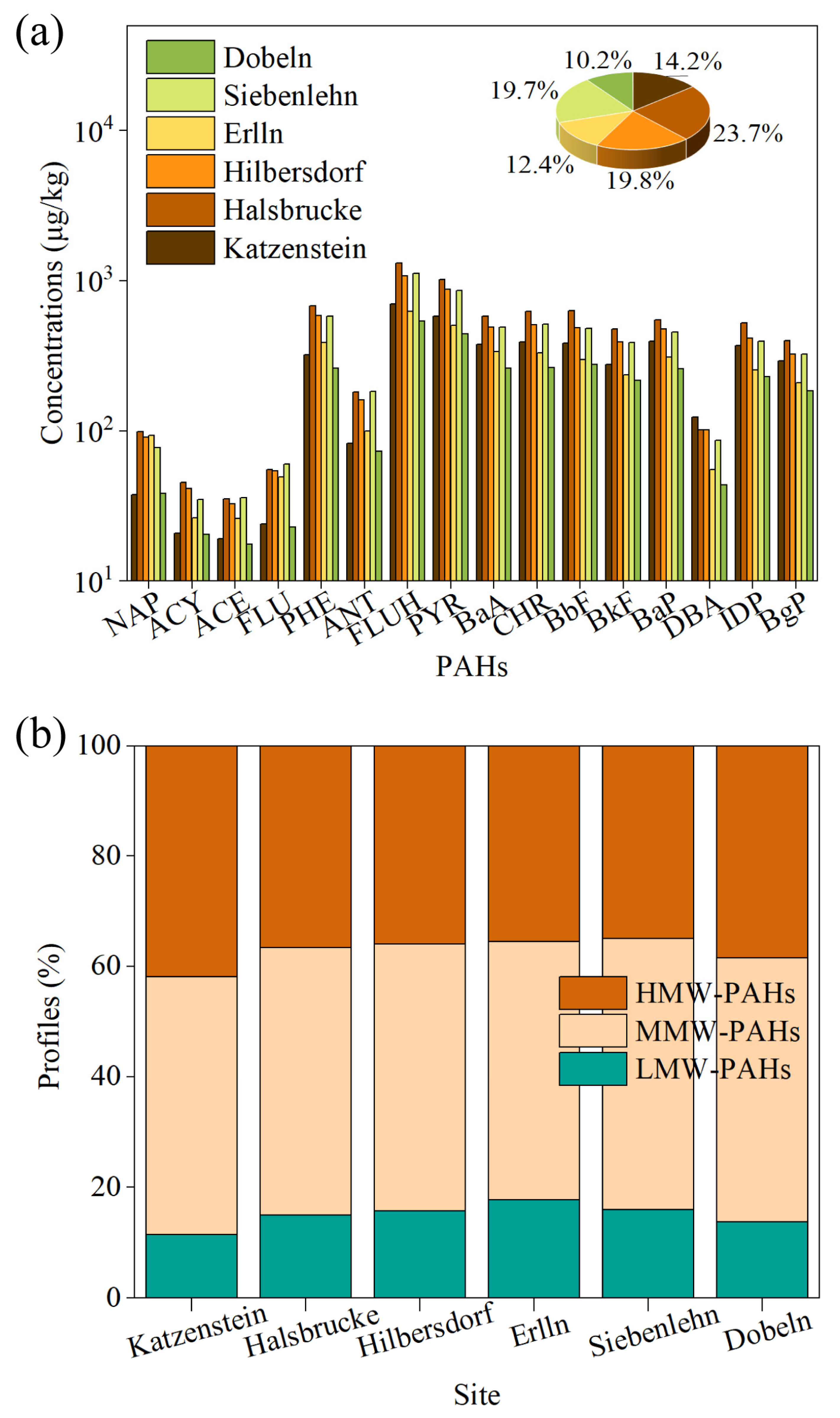
3.1. Distribution Characteristics of PAHs

As shown in Table 1, the general concentrations of Σ16PAHs in six stations during 2002–2016 ranged from 707.0 to 17,243.0 μg kg−1, with a mean value of 5258.0 ± 2569.2 μg kg−1. The multi-year average concentrations of individual PAHs rank as: FLUH (922.5 ± 517.4 μg kg−1) > PYR (731.1 ± 392.6 μg kg−1) > PHE (496.6 ± 300.0 μg kg−1) > CHR (445.8 ± 220.5 μg kg−1) > BaA (431.2 ± 211.0 μg kg−1) > BbF (425.9 ± 206.7 μg kg−1) > BaP (409.6 ± 191.0 μg kg−1) > IDP (358.6 ± 195.5 μg kg−1) > BkF (335.5 ± 177.3 μg kg−1) > BgP (286.3 ± 144.1 μg kg−1) > ANT (140.0 ± 122.2 μg kg−1) > NAP (81.2 ± 83.8 μg kg−1) > DBA (80.8 ± 50.2 μg kg−1) > FLU (50.0 ± 50.1 μg kg−1) > ACY (33.1 ± 19.4 μg kg−1) > ACE (29.8 ± 20.9 μg kg−1). The value of the coefficient of variation (CV) represents the level of spatiotemporal variation in the concentration of Σ16PAHs. The relatively high values of CV were observed in the concentrations of ACE (2.9) and IDP (2.1), indicating that they might be related to a sudden pollution incident or point source pollution. Meanwhile, the relatively low one was observed in the concentrations of BbF (0.6) and BkF (0.6), which might be related to emissions from non-point sources.
The spatial distribution of the average annual concentration during 2002–2016 of Σ16PAHs at six stations in the Freiberger Mulde river is illustrated in Table 1. A similar average annual concentration was observed in Hilbersdorf, Halsbrucke, and Siebenlehn stations. The highest mean concentration of Σ16PAHs was in Halsbrucke (7297.5 μg kg−1), and the second-highest value was located in Hilbersdorf (6096.9 μg kg−1). High concentration levels of PAHs suggested that these stations might be strongly influenced by anthropogenic activity. Meanwhile, the lowest mean concentration of Σ16PAHs was observed in Dobeln (3147.8 μg kg−1). The higher PAHs concentration levels were mainly distributed in the upstream of the river, which indicated that there were obvious spatial differences in the emission sources of PAHs.
Figure 2 showed the annual changes in the concentrations of Σ16PAHs from 2002 to 2016. The annual average concentration of PAHs decreased from 5457.0 μg kg−1 in 2002 to 3095.0 μg kg−1 in 2016. In addition, Mann–Kendall trend analysis was used to explore the long-term trends of Σ16PAHs concentrations from 2002 to 2016. The results suggested that the PAHs pollution level in the river decreased significantly during the period (confidence level = 97.7% and slope = −198.6). In addition, the maximum and minimum annual average concentrations of PAHs appeared in 2009 and 2012, respectively. Two extremely high PAHs concentration levels were observed (up to 57,480.0 and 55,950.0 μg kg−1, respectively) monitored at the Hilbersdorf site in 2009, which might be related to a special pollution event at the station.
Compared to research globally, the concentration of PAHs in suspended particulates in the Freiberger Mulde river was comparable to Victoria Harbour (China) [53], Kaohsiung Harbor (China) [54], Pearl River Estuary (China) [55], and Henan Reach of Yellow River (China) [56]; higher than Taranto Gulf (Italy) [57], Incheon Harbor (Korea) [58] and Hun River (China) [23]; and significantly lower than Xiamen Harbor (China) [53], Boston Harbor (USA) [59], Norwegian Harbor (Norway) [60] and Western Harbour (Egypt) [61] (Table S3). Following the general practice for the determination of relative rates of emissions [62], four levels of contamination can be divided: (1) low level: 0.0–100.0 μg kg−1; (2) moderate level: 100.0–1000.0 μg kg−1; (3) high level: 1000.0–5000.0 μg kg−1; and (4) very high level: >5000.0 μg kg−1. Accordingly, the PAH concentration in the suspended particulate matter from the Freiberger Mulde river from 2002 to 2016 was cataloged as high to very high levels, indicating the moderate-high PAHs pollution in the study river.

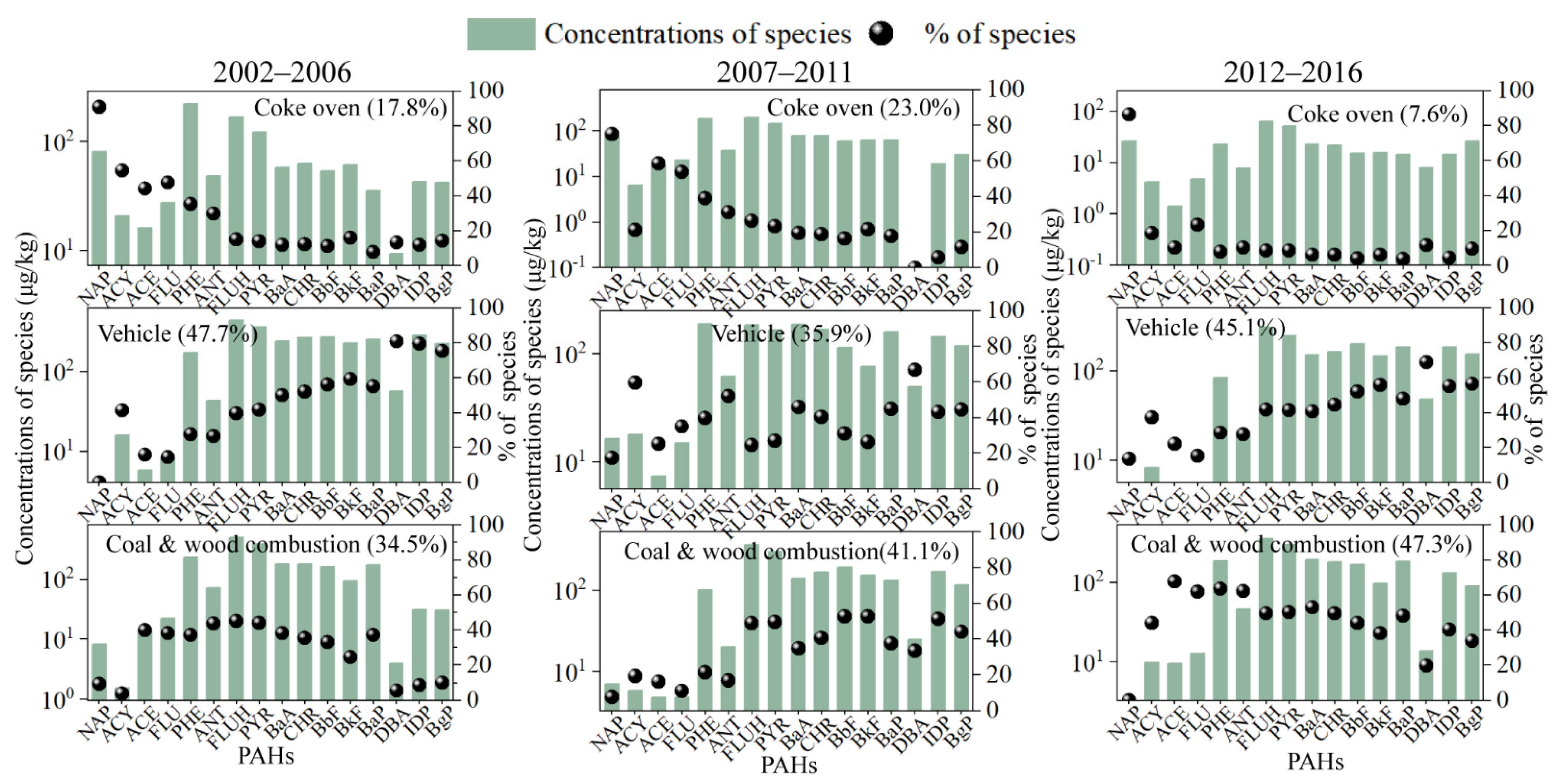
3.2. Composition Profiles of PAHs

Figure 3a shows the profile of the benzene-member ring of Σ16PAHs in different stations. The maximum proportion of PAHs was found in station Halsbrucke (23.7%), followed by stations Hilbersdorf (19.8%), and Katzenstein (14.2%). In addition, the proportion of PAHs with various ring numbers in Σ16PAHs in different stations is illustrated in Figure 3b. These 16 PAHs were commonly classified into three classes based on the number of benzene rings: low molecular weight (LMW, 2–3 rings) (NAP, ACE, ACY, FLU, ANT, PHE), middle molecular weight (MMW, four rings) (FLUH, PYR, BaA, CHR) and high molecular weight (HMW, 5–6 rings) (BaP, BbF, BkF, BgP, IDP, DBA). The annual average concentration of the MMW-PAHs ranged from 1505.0 to 3530.0 μg kg−1; that of the HMW-PAHs ranged from 1209.6 to 2675.2 μg kg−1, and that of the LMW-PAHs ranged from 433.2 to 1092.3 μg kg−1.
Previous studies have reported the composition of PAHs in suspended sediments from other rivers. In developing countries, the content of LMW-PAHs in river water environments is usually higher. For example, LMW-PAHs dominated the suspended sediments in the Pearl River Estuary, followed by MMW-PAHs [63]; MMW-PAHs dominated the suspended sediments of the Subarnarekha River in India, followed by LMW-PAHs [64]. In developing countries, biomass burning remains an important source of energy [65,66]. The high proportion of LMW-PAHs in these rivers might be associated with higher-intensity biomass burning emissions nearby.
The higher proportions of high molecular weight PAHs might be indicative of anthropogenic influences from higher urbanization. In this study, the MMW-PAHs contributed the highest proportion of Σ16PAHs (46.6–49.1%) in all stations, while the HMW-PAHs contributed the second-highest proportion of Σ16PAHs (35.0–41.9%). Previous studies have shown that the spatial variances of MMW-PAHs and HMW-PAHs concentrations in the environment are highly positively correlated with the densities of industrial activities and traffic emissions, respectively [67,68]. The proportions of MMW-PAHs exhibited fewer spatial differences in the river. Meanwhile, the proportion of HMW-PAHs in the upstream site was significantly higher than that in the downstream site, and the highest proportion of LMW-PAHs appeared in the midstream site. Therefore, the study river might be heavily polluted by emissions from upstream urban traffic and industrial activities. In addition, studies have shown that the Elbe is highly polluted by HMW-PAHs [1]. As one of the important tributaries flowing into the Elbe, the Freiberger Mulde river is one of the important input sources of PAHs with a high ring number. However, the above analysis indicates that the higher content of HMW-PAHs in the river might be attributed to upstream input.

3.3. Source Apportionment Derived by PMF

In this study, the long-term PAHs concentration dataset was divided into three parts: 2002–2006, 2007–2011, and 2012–2016. Quantitative source identification of Σ16PAHs in different periods was performed using the PMF model to investigate the characteristics of the variation in the number and intensity of PAHs sources over the years. Table S4 lists the correlation coefficient (R2) values between observed and predicted PAHs concentrations of the PMF model [69]. All the values of R2 were greater than 0.6, which indicated that the PMF model had a high prediction accuracy for the source apportionment of PAHs in the river.
The PMF model results are illustrated in Figure 4. The model identified three potential sources of Σ16PAHs during the study period. Factor 1 counted for 7.6–23.0% of the total PAH concentrations. This factor was dominated by a high portion of NAP and a relatively high portion of FLU. The NAP was the predominant PAHs of the coke oven [70]. Moreover, FLU was the important tracer of PAHs emitted from the coke ovens in Chicago [6]. Thus, this factor was denoted as a coke oven. Factor 2 counted for 35.9–47.7% of the total PAHs concentrations, and it was dominated by BbF, BkF, BaP, BgP, IDP, and DBA. The high loading of BgP was suggested as the traces of vehicular emissions, especially in gasoline engines [6,71]. The high weighting of BbF and BkF represented the emissions from diesel-power vehicles [72]. In addition, the high content of IDP was mostly observed in emissions of the high-way tunnel and vehicle engines [70]. Therefore, factor 2 was denoted as vehicle emissions in this study. Factor 3 counted for 34.5–47.3% of the total PAHs concentrations. This factor was characterized by FLUH, ACE, PYR, and ANT. High concentrations of alkyl PAHs (such as FLUH, ACE, and PYR) were the predominant tracers of coal combustion [6]. The dominance of HHW-PAHs in this factor also indicated that this factor was highly related to industrial coal combustion (high-temperature combustion processes) [73]. Moreover, ANT was the important tracer of wood combustion [72]. Thus, factor 3 was identified as coal and wood combustion.
In addition, the results were compared with the source analysis results of PAHs in other rivers. In developing countries, coal and biomass are often the main sources of energy supply. For example, the main sources of PAHs in the seven major river basins in China and the Guanlan River (China) are coal and biomass combustion (source contributions account for 40.0% and 42.8% of the total, respectively) [74,75]. In the more urbanized developed countries, the proportion of traffic emissions is usually higher. The main sources of PAHs in the Heihe and Ashtabula Rivers (Ohio) and Brisbane Rivers (Australia) were characterized by traffic emissions (source contributions accounted for 58.0% and 42.8% of the total, respectively) [76,77]. In this study, the contributions of coal and biomass combustion and traffic emission sources are similar. The unexpectedly high portion of coal and biomass combustion sources might be attributed to the relatively low level of industrialization in the cities along the river.
In addition, the results of displacement (DISP) and bootstrap (BS) were used to evaluate the stability of the PMF model (Table S5). The matching rates of BS runs in all PMF models were over 80%, which indicated that the random errors of the models were sufficiently small to be acceptable [4,34]. In addition, the DISP was mainly developed to analyze the rotational ambiguity of the PMF model results. No swapped factors were observed in the DISP running of all PMF models, and the decrease in Q value was within a reasonable range [4]. Therefore, the above results indicated that the PMF model in this study was sufficiently stable and reliable enough to be accepted.

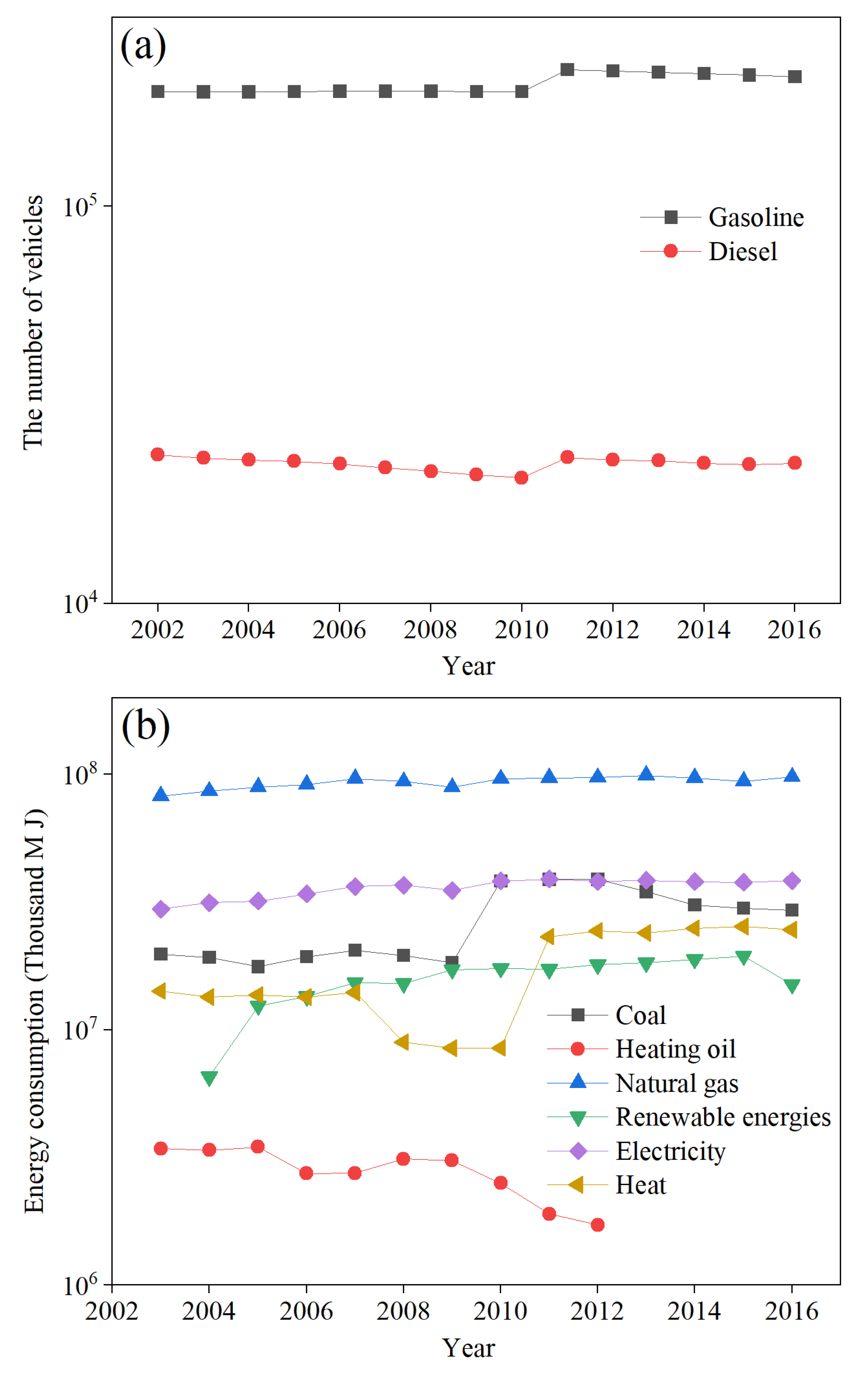
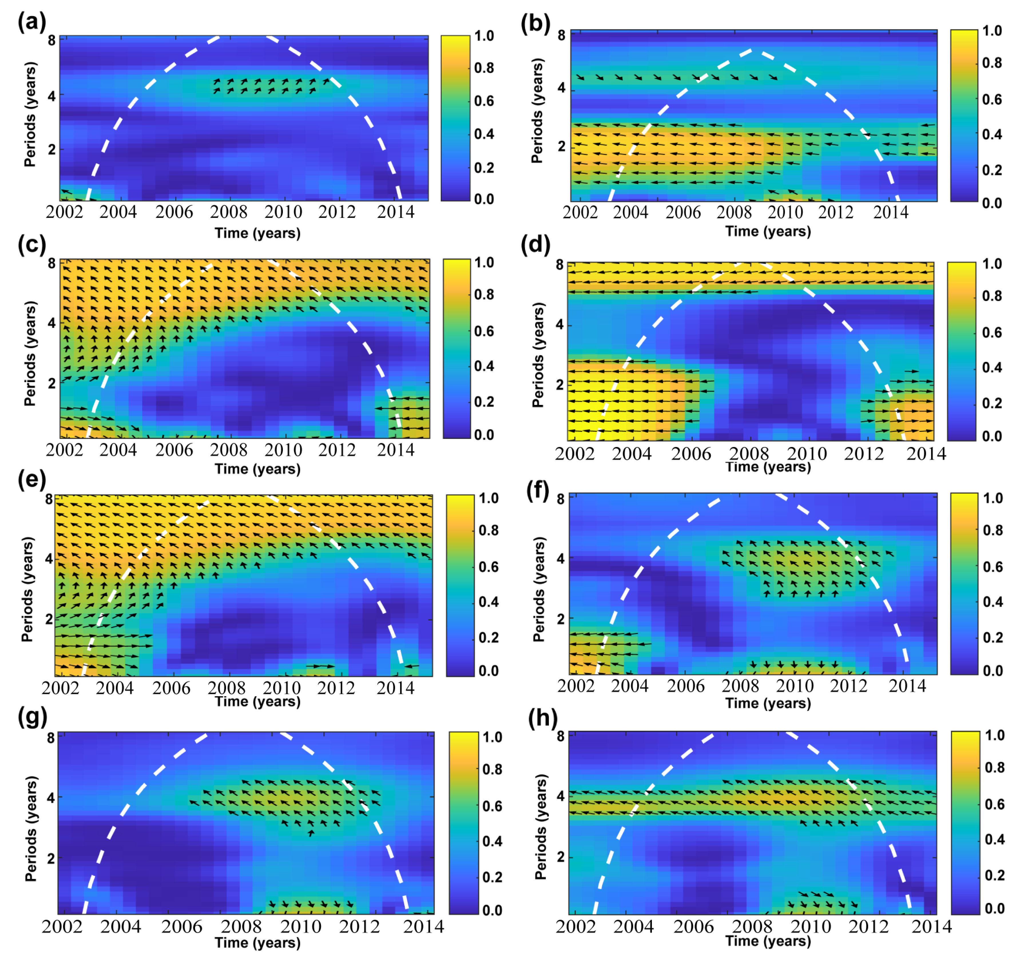
3.4. Potential Driving Force of PAHs

The quantitative source apportionment results of PMF indicated that the pollution levels of PAHs in urban rivers were mainly affected by anthropogenic activities. The contributions to PAHs concentrations in the Freiberger Mulde river from different sources vary significantly over time (Figure 5). Furthermore, the results of wavelet coherence revealed the detailed effects of various anthropogenic activities on the concentrations of PAHs in suspended sediments (Figure 6). The numerical range for judging the value of wavelet coherence (WC) is between 0 and 1, and the larger value indicates a stronger correlation. Arrows to the left and right represent positive and inverse correlations, respectively.
The contribution of coke ovens increased from 17.8% in 2002–2006 to 23.0% in 2007–2011 and then dropped to 7.6% in 2012–2016 (Figure 4). Coal is a critical raw material and energy source in the coke oven industry. The annual changes in energy consumption of various types of energy in Saxony from 2003 to 2016 were shown in Figure 5b. The value of coal consumption increased substantially in 2009–2010 and then declined over time after 2010. The reduction in coal consumption in recent years was related to the government’s vigorous promotion of clean energy [1,78]. The variation pattern of the coke oven was similar to that of the coal consumption sequence, indicating that the decreased contribution of the coke oven to the PAHs pollution in the study area might be attributed to the reduction in the use of coal products. In addition, the positive effects of coal consumption on PAHs emissions in the study area with a time scale of 5–6 years were observed from 2007 to 2011 (Figure 6a). The reduction in industrial coal consumption in recent years might be attributed to the European directives to limit emissions of PAHs in 2008 (2008/50/EC) and 2010 (2010/75/EU) [79,80]. However, the strength of WC was insignificant, which might indicate that variations in PAH concentrations in the river might be mainly influenced by emission sources outside the study area (e.g., upstream input). Besides, combining the analysis in Section 3.2 and other studies, the MMW-PAHs from industrial emissions (especially coal-fired power plants and the thriving mining industry) in the river might originate from the emissions in upstream [39,81].
In addition, the contribution of coal and wood combustion sources increased from 34.5% in 2002–2006 to 41.1% in 2007–2011, and then to 47.3% in 2012–2016 (Figure 4). Similar to the coke oven source, the increase in the contribution from this source between 2007 and 2011 might be related to the increase in coal consumption (Figure 5b). In addition, despite how clean energy was gradually used to replace fossil fuels in recent years, the combustion of traditional fuels (such as wood, coal, and fuel oil) was still the main source of heating for residents in the cold season [78]. The wavelet coherence results showed that the strong negative effect of fuel oil used for heating on PAHs emission appeared during 2002–2007 (Figure 6b). Fuel oil consumption for heating had dropped significantly during the period. The decrease in the use of heating oil has led to an increase in the use of traditional fuels. Research showed that the change in heating energy structure is related to the economic ability of residents [78]. The sudden change in economic conditions in 2008 led to the increase in the use of cheaper fuels in household life, which might be the important reason for the increased contribution from wood and coal combustion intensity during 2012–2016.
However, the contribution of vehicle emission sources showed a different pattern of change. The contribution of the source decreased from 47.7% in 2002–2006 to 35.9% in 2007–2011 and then increased to 45.1% in 2012–2016 (Figure 4). Figure 5a illustrates the change in the number of gasoline and diesel vehicles from 2002 to 2016. During 2002–2010, the number of diesel vehicles showed an obvious downward trend, while the number of both gasoline and diesel vehicles increased significantly after 2010. The wavelet coherence results also showed that the increase in the number of gasoline and diesel vehicles (Figure 6g,h) around 2010 had a significant positive effect on the emissions of PAHs (the relatively high WC values located in 2010–2012 with the time scale of 0–1 years). Besides, the wavelet coherence results showed that the negative effects of gasoline vehicles (Figure 6g) and diesel vehicles (Figure 6h) were concentrated in 2009–2013 and 2002–2013, respectively [71]. Using negative correlations to describe the changes in the number of cars and PAHs concentrations is inaccurate. The factors that affect the intensity of traffic emissions are often complex, especially over longer periods. Previous studies suggested that there was an obvious positive correlation between the concentration of PAHs in the urban water environment and the number of vehicles [82,83]. The implementation of vehicle emission reduction strategies and technologies in recent years could reduce the traffic emissions of PAHs (Euro 4 in 2005 and Euro 5 in 2009) [84,85]. In addition, reducing the proportion of PAHs in fuel was also an effective emission reduction measure [86]. In future work, it might be more appropriate to use estimated vehicle PAHs emissions to investigate their effects on the changes in PAHs concentrations, especially in studies on long-term changes in PAHs.
During the study period, the consumption of natural gas (Figure 6c), renewable energy (Figure 6d), and electricity (Figure 6e) had a very significant negative effect on the concentration of PAHs in suspended sediments on a time scale of 6–8 years. Compared with renewable energy, the increase in the use of natural gas and electric energy has a more significant effect on the decrease in PAHs concentration in river suspended sediments, which might be due to the fact that their consumption is significantly higher than that of renewable energy. On the other hand, natural gas is mainly used for household combustion activities, which greatly reduces the use of other high PAHs emitting fuels. These results indicate that the further promotion of renewable energy will play a crucial role in reducing PAHs emissions in the future.

3.5. Risk Assessment of PAHs

3.5.1. Potential Biological Effects

This study used the ERL and ERM values to comprehensively assess the potential ecological risk of Σ16PAHs in the suspended particulate matter of the Freiberger Mulde river (Table S6). The average concentrations of NAP, ACY, and ANT were 101.0 μg kg−1, 39.0 μg kg−1, and 170.0 μg kg−1, lower than the respective ERL values of 38.6%, 11.3%, and 80.0%, respectively. However, the average value of the other PAHs ranged within the values of ERL and ERM. The maximum values of PHE and DBA were 2000.0 μg kg−1 and 1100.0 μg kg−1, respectively, which were higher than their respective ERM values of 25.0% and 76.3%. Excluding PHE and DBA, the maximum PAHs concentrations were lower than their respective ERM values. This indicated that the ecosystem of the Freiberger Mulde river might have been threatened by PAHs during the study period, which was mainly attributed to the high concentrations of PHE and DBA caused by unexpected events (such as flooding).
Table S7 summarizes the MHQs and HQs for the components of Σ16PAHs at different stations. The total PAHs in the suspended particulate matter of the Freiberger Mulde river were commonly dominated by MMW-PAHs and HMW-PAHs. The MHQ in six stations ranged from 0.1 to 0.3; the maximum MHQ (0.3) was observed at the Hilbersdorf station. The HQs of PHE and DBA at the Hilbersdorf station were higher than other PAHs. This evidence indicated that the contamination of PHE and DBA needed considerable attention, which was mainly generated by coke ovens and vehicle emissions. In addition, in this study, all MHQ values (0.1–0.3) were in the range of 0.11 to 0.5, which corresponds to a 21.0% probability of toxicity to benthic fauna [87]. The results represented that the Σ16PAHs in the river might have adversely affected the benthic fauna of the Freiberger Mulde river and the aquatic environment.

3.5.2. Potential Human Toxicity

The total TEQ calculated for Σ16PAH in the study area varied from 407.0 to 1180.0 μg kg−1 dry weight (Table 2). The highest TEQ value was observed at Halsbrucke station, which is located in the middle of the Freiberger Mulde river and was close to urban and commercial areas. The TEQ values declined from upstream to downstream of the river. On the one hand, it might be related to the fact that the emission sources of PAHs were concentrated in upstream. On the other hand, it might be also related to the degradation and dilution of PAHs (especially LMW-PAHs) during the migration of rivers [88].
The values and percentage contributions of TEQ of each PAHs are summarized in Table 2. The contributions of TEQ of individual PAHs were ranked in the following order: FLUH (16.0–18.4%) > PYR (13.1–15.2%) > PHE (7.3–11.9%) > CHR (7.6–9.0%) > BaP (5.4–9.0%) > BaA (7.4–8.8%) > BbF (6.7–8.6%) > IDP (5.9–8.2%) > BgP (5.3–8.0%) > BkF (5.4–6.9%) > other PAHs (less than 3.0%). MMW-PAHs and HMW-PAHs, which mainly originated from fossil fuel combustion, accounted for most of the total TEQ values in the river. Thus, the relatively high TEQ values in river suspensions during the study period were highly correlated with vehicle emissions and coal and wood combustion.
The values for TEQ in the suspended particulate matter from other studies are presented in Table S8. The TEQ values (407.0–1180.0 μgTEQ/kg dry wt.) in this study were lower than those in Naples Harbor (69.0–18,681.0 μgTEQ/kg dry wt.) (Italy) and Kaohsiung Harbor (55.0–1964.0 μgTEQ/kg dry wt.), but were higher than those in Meiliang Bay (94.0–845.0 μgTEQ/kg dry wt.) (China), Eastern Mediterranean Sea (17.0–872.0 μgTEQ/kg dry wt.) (Lebanon), and Barents Sea (638.0–1777.0 μgTEQ/kg dry wt.) (Russia). Overall, the average potential toxicity risk in the suspended particulate matter of the Freiberger Mulde river was moderate for humans from 2002 to 2016 compared to other rivers.

4. Conclusions

This study investigated the concentration levels, spatiotemporal variances, potential sources, and their driving forces, as well as ecological and human health risk assessments of Σ16PAHs in suspended particulates of typical surface water. The concentrations of Σ16PAHs in the study area were at moderate-high pollution levels. Higher concentrations of Σ16PAHs were concentrated in the midstream and upstream of the river. The concentration of Σ16PAHs in the suspension showed an obvious decreasing pattern with time. The PMF receptor model identified three potential PAH sources of coke ovens, vehicle emissions, and coal and wood combustion. Results indicated that the changes in the energy structure had a greater impact on the changes in contributions of these sources during 2002–2016. The ecological risk and human health assessment showed that a higher risk of PAHs in the given river during 2002–2016 was mainly influenced by special pollution events. The PAHs emitted from vehicle emission and coal and wood combustion posed a threat to the aquatic organisms and human health. The data provided herein suggest that policymakers might need to increase the proportion of clean energy use to reduce the pollution levels of PAHs in the water environment.

Supplementary Materials

The following supporting information can be downloaded at: https://www.mdpi.com/article/10.3390/su14116646/s1, Section S2: Sample analysis [32]; Season S2: Mann-Kendall trend test [89,90,91]; Season S3: Wavelet analysis [1,45,92,93,94]; Table S1: The sampling information for stations; Table S2: Proposed toxicity equivalency factors (TEFs) for individual PAHs; Table S3: Global review of PAHs concentrations [23,53,54,55,56,57,58,59,60,61,83,95,96,97,98,99,100,101,102,103,104,105,106,107]; Table S4: The correlation coefficient (R2) values between observed and predicted concentrations of the PMF model; Table S5: The results of Displacement (DISP) and Bootstrap (BS) by PMF model; Table S6: Effects range-low (ERL), effects range-median (ERM), mean and maximum concentration of 16 PAHs in μg kg-1; Table S7: Hazard quotients (HQ) and mean hazard quotient (MHQ) of 16 PAHs from 2002-2016; Table S8: TEQ values of PAHs at different locations [54,83,108,109,110].

Author Contributions

Data curation, Z.Q., Y.L. and J.X.; Methodology, Z.Q. and Z.W.; Project administration, J.Z.; Writing—original draft, Z.Q.; Writing—review & editing, J.Z. All authors have read and agreed to the published version of the manuscript.

Funding

This research was jointly funded by [“Collaborative early warning information systems for urban infrastructures (COLABIS)” funded by Bundesministerium für Bildung und Forschung] grant number [03G0852A]; and [“Advanced technologies for water distribution system management” funded by Deutscher Akademischer Austauschdienst] grant number [PROBRAL57273574].

Acknowledgments

The authors would like to gratefully thank the Saxony State Office for Environment, Agriculture and Geology (Landesamt für Umwelt, Landwirtschaft und Geologie, LfULG) for providing the data and the Public Operating Company for Environment and Agriculture (Staatliche Betriebsgesellschaft für Umwelt und Landwirtschaft, BfUL) for measuring the data. This manuscript has not been subjected to the above agencies’ required peer and policy review and therefore does not reflect the views of the above agencies and no official endorsement should be inferred.

Conflicts of Interest

The authors declare no conflict of interest.

References

  1. Li, R.; Hua, P.; Zhang, J.; Krebs, P. Effect of anthropogenic activities on the occurrence of polycyclic aromatic hydrocarbons in aquatic suspended particulate matter: Evidence from Rhine and Elbe Rivers. Water Res. 2020, 179, 115901. [Google Scholar] [CrossRef]
  2. Meng, Y.; Liu, X.; Lu, S.; Zhang, T.; Jin, B.; Wang, Q.; Tang, Z.; Liu, Y.; Guo, X.; Zhou, J.; et al. A review on occurrence and risk of polycyclic aromatic hydrocarbons (PAHs) in lakes of China. Sci. Total. Environ. 2019, 651, 2497–2506. [Google Scholar] [CrossRef]
  3. Dong, L.; Zhang, J. Predicting polycyclic aromatic hydrocarbons in surface water by a multiscale feature extraction-based deep learning approach. Sci. Total Environ. 2021, 799, 149509. [Google Scholar] [CrossRef]
  4. Norris, G.; Duvall, R.; Brown, S.; Bai, S. EPA Positive Matrix Factorization (PMF) 5.0 Fundamentals and User Guide; EPA/600/R-14/108; U.S. Environmental Protection Agency: Washington, DC, USA, 2014; pp. 1–136. [Google Scholar]
  5. Manoli, E.; Samara, C.; Konstantinou, I.; Albanis, T. Polycyclic aromatic hydrocarbons in the bulk precipitation and surface waters of Northern Greece. Chemosphere 2000, 41, 1845–1855. [Google Scholar] [CrossRef]
  6. Simcik, M.F.; Eisenreich, S.J.; Lioy, P.J. Source apportionment and source/sink relationships of PAHs in the coastal atmosphere of Chicago and Lake Michigan. Atmos. Environ. 1999, 33, 5071–5079. [Google Scholar] [CrossRef]
  7. Lohmann, R.; Gioia, R.; Jones, K.C.; Nizzetto, L.; Temme, C.; Xie, Z.; Schulz-Bull, D.; Hand, I.; Morgan, E.; Jantunen, L. Organochlorine Pesticides and PAHs in the Surface Water and Atmosphere of the North Atlantic and Arctic Ocean. Environ. Sci. Technol. 2009, 43, 5633–5639. [Google Scholar] [CrossRef]
  8. Lin, Y.; Qiu, X.; Ma, Y.; Ma, J.; Zheng, M.; Shao, M. Concentrations and spatial distribution of polycyclic aromatic hydrocarbons (PAHs) and nitrated PAHs (NPAHs) in the atmosphere of North China, and the transformation from PAHs to NPAHs. Environ. Pollut. 2015, 196, 164–170. [Google Scholar] [CrossRef]
  9. Tan, X.; Yu, X.; Cai, L.; Wang, J.; Peng, J. Microplastics and associated PAHs in surface water from the Feilaixia Reservoir in the Beijiang River, China. Chemosphere 2019, 221, 834–840. [Google Scholar] [CrossRef]
  10. Bao, K.; Zaccone, C.; Tao, Y.; Wang, J.; Shen, J.; Zhang, Y. Source apportionment of priority PAHs in 11 lake sediment cores from Songnen Plain, Northeast China. Water Res. 2019, 168, 115158. [Google Scholar] [CrossRef]
  11. Dudhagara, D.R.; Rajpara, R.K.; Bhatt, J.K.; Gosai, H.B.; Sachaniya, B.K.; Dave, B.P. Distribution, sources and ecological risk assessment of PAHs in historically contaminated surface sediments at Bhavnagar coast, Gujarat, India. Environ. Pollut. 2016, 213, 338–346. [Google Scholar] [CrossRef]
  12. Zhang, Y.; Guo, C.S.; Xu, J.; Tian, Y.Z.; Shi, G.L.; Feng, Y.C. Potential source contributions and risk assessment of PAHs in sediments from Taihu Lake, China: Comparison of three receptor models. Water Res. 2012, 46, 3065–3073. [Google Scholar] [CrossRef]
  13. Lang, Y.H.; Li, G.L.; Wang, X.M.; Peng, P. Combination of Unmix and PMF receptor model to apportion the potential sources and contributions of PAHs in wetland soils from Jiaozhou Bay, China. Mar. Pollut. Bull. 2015, 90, 129–134. [Google Scholar] [CrossRef]
  14. Huang, Z.; Liu, Y.; Dai, H.; Gui, D.; Hu, B.X.; Zhang, J. Spatial distribution and source apportionment of polycyclic aromatic hydrocarbons in typical oasis soil of north-western China and the bacterial community response. Environ. Res. 2021, 204, 112401. [Google Scholar] [CrossRef]
  15. Wilcke, W. SYNOPSIS Polycyclic Aromatic Hydrocarbons (PAHs) in Soil. J. Plant Nutr. Soil Sci. 2000, 163, 229–248. [Google Scholar] [CrossRef]
  16. Zhang, J.; Li, R.; Zhang, X.; Bai, Y.; Cao, P.; Hua, P. Vehicular contribution of PAHs in size dependent road dust: A source apportionment by PCA-MLR, PMF, and Unmix receptor models. Sci. Total Environ. 2018, 649, 1314–1322. [Google Scholar] [CrossRef]
  17. Majumdar, D.; Rajaram, B.; Meshram, S.; Chalapati Rao, C.V. PAHs in Road Dust: Ubiquity, Fate, and Summary of Available Data. Crit. Rev. Environ. Sci. Technol. 2012, 42, 1191–1232. [Google Scholar] [CrossRef]
  18. Soltani, N.; Keshavarzi, B.; Moore, F.; Tavakol, T.; Lahijanzadeh, A.R.; Jaafarzadeh, N.; Kermani, M. Ecological and human health hazards of heavy metals and polycyclic aromatic hydrocarbons (PAHs) in road dust of Isfahan metropolis, Iran. Sci. Total Environ. 2015, 505, 712–723. [Google Scholar] [CrossRef]
  19. Liu, M.; Cheng, S.B.; Ou, D.N.; Hou, L.J.; Gao, L.L.; Wang, L.; Xie, Y.S.; Yang, Y.; Xu, S.Y. Characterization, identification of road dust PAHs in central Shanghai areas, China. Atmos. Environ. 2007, 41, 8785–8795. [Google Scholar] [CrossRef]
  20. Huang, Y.; Sun, X.; Liu, M.; Zhu, J.; Yang, J.; Du, W.; Zhang, X.; Gao, D.; Qadeer, A.; Xie, Y.; et al. A multimedia fugacity model to estimate the fate and transport of polycyclic aromatic hydrocarbons (PAHs) in a largely urbanized area, Shanghai, China. Chemosphere 2018, 217, 298–307. [Google Scholar] [CrossRef]
  21. Du, J.; Jing, C. Anthropogenic PAHs in lake sediments: A literature review (2002–2018). Environ. Sci. Process. Impacts 2018, 20, 1649–1666. [Google Scholar] [CrossRef]
  22. Wang, C.; Zou, X.; Zhao, Y.; Li, B.; Song, Q.; Li, Y.; Yu, W. Distribution, sources, and ecological risk assessment of polycyclic aromatic hydrocarbons in the water and suspended sediments from the middle and lower reaches of the Yangtze River, China. Environ. Sci. Pollut. Res. 2016, 23, 17158–17170. [Google Scholar] [CrossRef]
  23. Guo, W.; He, M.; Yang, Z.; Lin, C.; Quan, X.; Wang, H. Distribution of polycyclic aromatic hydrocarbons in water, suspended particulate matter and sediment from Daliao River watershed, China. Chemosphere 2007, 68, 93–104. [Google Scholar] [CrossRef]
  24. Li, G.; Xia, X.; Yang, Z.; Wang, R.; Voulvoulis, N. Distribution and sources of polycyclic aromatic hydrocarbons in the middle and lower reaches of the Yellow River, China. Environ. Pollut. 2006, 144, 985–993. [Google Scholar] [CrossRef]
  25. Yang, D.; Qi, S.; Zhang, Y.; Xing, X.; Liu, H.; Qu, C.; Liu, J.; Li, F. Levels, sources and potential risks of polycyclic aromatic hydrocarbons (PAHs) in multimedia environment along the Jinjiang River mainstream to Quanzhou Bay, China. Mar. Pollut. Bull. 2013, 76, 298–306. [Google Scholar] [CrossRef]
  26. Shi, G.L.; Zeng, F.; Li, X.; Feng, Y.C.; Wang, Y.Q.; Liu, G.X.; Zhu, T. Estimated contributions and uncertainties of PCA/MLR–CMB results: Source apportionment for synthetic and ambient datasets. Atmos. Environ. 2011, 45, 2811–2819. [Google Scholar] [CrossRef]
  27. Song, Y.; Xie, S.; Zhang, Y.; Zeng, L.; Salmon, L.G.; Zheng, M. Source apportionment of PM2.5 in Beijing using principal component analysis/absolute principal component scores and UNMIX. Sci. Total Environ. 2006, 372, 278–286. [Google Scholar] [CrossRef]
  28. Lee, S.; Russell, A.G. Estimating uncertainties and uncertainty contributors of CMB PM2.5 source apportionment results. Atmos. Environ. 2007, 41, 9616–9624. [Google Scholar] [CrossRef]
  29. Sheesley, R.J.; Schauer, J.J.; Zheng, M.; Wang, B. Sensitivity of molecular marker-based CMB models to biomass burning source profiles. Atmos. Environ. 2007, 41, 9050–9063. [Google Scholar] [CrossRef]
  30. Dai, Q.; Hopke, P.K.; Bi, X.; Feng, Y. Improving apportionment of PM2.5 using multisite PMF by constraining G-values with a prioriinformation. Sci. Total Environ. 2020, 736, 139657. [Google Scholar] [CrossRef]
  31. Bhuiyan, M.A.H.; Karmaker, S.C.; Doza, B.; Rakib, A.; Saha, B.B. Enrichment, sources and ecological risk mapping of heavy metals in agricultural soils of dhaka district employing SOM, PMF and GIS methods. Chemosphere 2020, 263, 128339. [Google Scholar] [CrossRef]
  32. Li, R.; Cai, J.; Li, J.; Wang, Z.; Pei, P.; Zhang, J.; Krebs, P. Characterizing the long-term occurrence of polycyclic aromatic hydrocarbons and their driving forces in surface waters. J. Hazard. Mater. 2021, 423, 127065. [Google Scholar] [CrossRef] [PubMed]
  33. Brown, S.G.; Eberly, S.; Paatero, P.; Norris, G.A. Methods for estimating uncertainty in PMF solutions: Examples with ambient air and water quality data and guidance on reporting PMF results. Sci. Total Environ. 2015, 518–519, 626–635. [Google Scholar] [CrossRef] [PubMed] [Green Version]
  34. Paatero, P.; Hopke, P.K.; Song, X.-H.; Ramadan, Z. Understanding and controlling rotations in factor analytic models. Chemom. Intell. Lab. Syst. 2002, 60, 253–264. [Google Scholar] [CrossRef]
  35. Zanotti, C.; Rotiroti, M.; Fumagalli, L.; Stefania, G.A.; Canonaco, F.; Stefenelli, G.; Prévôt, A.S.H.; Leoni, B.; Bonomi, T. Groundwater and surface water quality characterization through positive matrix factorization combined with GIS approach. Water Res. 2019, 159, 122–134. [Google Scholar] [CrossRef]
  36. Liu, R.; Men, C.; Yu, W.; Xu, F.; Wang, Q.; Shen, Z. Uncertainty in positive matrix factorization solutions for PAHs in surface sediments of the Yangtze River Estuary in different seasons. Chemosphere 2018, 191, 922–936. [Google Scholar] [CrossRef]
  37. Yang, B.; Zhou, L.; Xue, N.; Li, F.; Li, Y.; Vogt, R.D.; Cong, X.; Yan, Y.; Liu, B. Source apportionment of polycyclic aromatic hydrocarbons in soils of Huanghuai Plain, China: Comparison of three receptor models. Sci. Total Environ. 2013, 443, 31–39. [Google Scholar] [CrossRef]
  38. Salim, I.; Sajjad, R.U.; Paule-Mercado, M.C.; Memon, S.A.; Lee, B.-Y.; Sukhbaatar, C.; Lee, C.-H. Comparison of two receptor models PCA-MLR and PMF for source identification and apportionment of pollution carried by runoff from catchment and sub-watershed areas with mixed land cover in South Korea. Sci. Total Environ. 2019, 663, 764–775. [Google Scholar] [CrossRef]
  39. Tichomirowa, M.; Heidel, C.; Junghans, M.; Haubrich, F.; Matschullat, J. Sulfate and strontium water source identification by O, S and Sr isotopes and their temporal changes (1997–2008) in the region of Freiberg, central-eastern Germany. Chem. Geol. 2010, 276, 104–118. [Google Scholar] [CrossRef]
  40. Schreiber, M.; Otto, M.; Fedotov, P.S.; Wennrich, R. Dynamic studies on the mobility of trace elements in soil and sediment samples influenced by dumping of residues of the flood in the Mulde River region in 2002. Chemosphere 2005, 61, 107–115. [Google Scholar] [CrossRef]
  41. Sprößig, C.; Buchholz, S.; Dziock, F. Defining the baseline for river restoration: Comparing carabid beetle diversity of natural and human-impacted riparian habitats. J. Insect Conserv. 2020, 24, 805–820. [Google Scholar] [CrossRef]
  42. Jiang, J.; Zheng, Y.; Pang, T.; Wang, B.; Chachan, R.; Tian, Y. A comprehensive study on spectral analysis and anomaly detection of river water quality dynamics with high time resolution measurements. J. Hydrol. 2020, 589, 125175. [Google Scholar] [CrossRef]
  43. Kang, S.; Lin, H. Wavelet analysis of hydrological and water quality signals in an agricultural watershed. J. Hydrol. 2007, 338, 1–14. [Google Scholar] [CrossRef]
  44. Zhang, J.; Zhang, X.; Niu, J.; Hu, B.X.; Soltanian, M.R.; Qiu, H.; Yang, L. Prediction of groundwater level in seashore reclaimed land using wavelet and artificial neural network-based hybrid model. J. Hydrol. 2019, 577. [Google Scholar] [CrossRef]
  45. Torrence, C.; Compo, G.P. A Practical Guide to Wavelet Analysis. Bull. Am. Meteorol. Soc. 1998, 79, 61–78. [Google Scholar] [CrossRef] [Green Version]
  46. Pejman, A.; Bidhendi, G.N.; Ardestani, M.; Saeedi, M.; Baghvand, A. A new index for assessing heavy metals contamination in sediments: A case study. Ecol. Indic. 2015, 58, 365–373. [Google Scholar] [CrossRef]
  47. Gu, Y.G.; Li, H.B.; Lu, H.B. Polycyclic aromatic hydrocarbons (PAHs) in surface sediments from the largest deep plateau lake in China: Occurrence, sources and biological risk. Ecol. Eng. 2017, 101, 179–184. [Google Scholar] [CrossRef] [Green Version]
  48. Cai, P.; Cai, G.; Chen, X.; Li, S.; Zhao, L. The concentration distribution and biohazard assessment of heavy metal elements in surface sediments from the continental shelf of Hainan Island. Mar. Pollut. Bull. 2021, 166, 112254. [Google Scholar] [CrossRef]
  49. Long, E.R.; Macdonald, D.D.; Smith, S.L.; Calder, F.D. Incidence of adverse biological effects within ranges of chemical concentrations in marine and estuarine sediments. Environ. Manag. 1995, 19, 81–97. [Google Scholar] [CrossRef]
  50. Pradeep, P.; Carlson, L.M.; Judson, R.; Lehmann, G.M.; Patlewicz, G. Integrating data gap filling techniques: A case study predicting TEFs for neurotoxicity TEQs to facilitate the hazard assessment of polychlorinated biphenyls. Regul. Toxicol. Pharmacol. 2018, 101, 12–23. [Google Scholar] [CrossRef]
  51. Savinov, V.M.; Savinova, T.N.; Matishov, G.G.; Dahle, S.; Næs, K. Polycyclic aromatic hydrocarbons (PAHs) and organochlorines (OCs) in bottom sediments of the Guba Pechenga, Barents Sea, Russia. Sci. Total Environ. 2003, 306, 39–56. [Google Scholar] [CrossRef]
  52. Sharma, M.D.; Elanjickal, A.I.; Mankar, J.S.; Krupadam, R.J. Assessment of cancer risk of microplastics enriched with polycyclic aromatic hydrocarbons. J. Hazard. Mater. 2020, 398, 122994. [Google Scholar] [CrossRef] [PubMed]
  53. Hong, H.; Xu, L.; Zhang, L.; Chen, J.C.; Wong, Y.S.; Wan, T.S.M. Special guest paper: Environmental fate and chemistry of organic pollutants in the sediment of Xiamen and Victoria Harbours. Mar. Pollut. Bull. 1995, 31, 229–236. [Google Scholar] [CrossRef]
  54. Chen, C.W.; Chen, C.F. Distribution, origin, and potential toxicological significance of polycyclic aromatic hydrocarbons (PAHs) in sediments of Kaohsiung Harbor, Taiwan. Mar. Pollut. Bull. 2011, 63, 417–423. [Google Scholar] [CrossRef] [PubMed]
  55. Luo, X.J.; Chen, S.J.; Mai, B.X.; Yang, Q.S.; Sheng, G.Y.; Fu, J.M. Polycyclic aromatic hydrocarbons in suspended particulate matter and sediments from the Pearl River Estuary and adjacent coastal areas, China. Environ. Pollut. 2006, 139, 9–20. [Google Scholar] [CrossRef]
  56. Sun, J.H.; Wang, G.L.; Chai, Y.; Zhang, G.; Li, J.; Feng, J. Distribution of polycyclic aromatic hydrocarbons (PAHs) in Henan Reach of the Yellow River, Middle China. Ecotoxicol. Environ. Saf. 2009, 72, 1614–1624. [Google Scholar] [CrossRef]
  57. Storelli, M.M.; Marcotrigiano, G.O. Polycyclic aromatic hydrocarbon distributions in sediments from the Mar Piccolo, Ionian Sea, Italy. Bull. Environ. Contam. Toxicol. 2000, 65, 537–544. [Google Scholar] [CrossRef]
  58. Kim, G.B.; Maruya, K.A.; Lee, R.F.; Lee, J.H.; Koh, C.H.; Tanabe, S. Distribution and Sources of Polycyclic Aromatic Hydrocarbons in Sediments from Kyeonggi Bay, Korea. Mar. Pollut. Bull. 1999, 38, 7–15. [Google Scholar] [CrossRef]
  59. Song, W.W.; He, K.B.; Wang, J.X.; Wang, X.T.; Shi, X.Y.; Yu, C.; Chen, W.M.; Zheng, L. Emissions of EC, OC, and PAHs from Cottonseed Oil Biodiesel in a Heavy-Duty Diesel Engine. Environ. Sci. Technol. 2011, 45, 6683–6689. [Google Scholar] [CrossRef]
  60. Oen, A.M.; Cornelissen, G.; Breedveld, G.D. Relation between PAH and black carbon contents in size fractions of Norwegian harbor sediments. Environ. Pollut. 2006, 141, 370–380. [Google Scholar] [CrossRef]
  61. Mostafa, A.R.; Barakat, A.O.; Qian, Y.; Wade, T.L. Composition, distribution and sources of polycyclic aromatic hydrocarbons in sediments of the western harbour of alexandria, egypt. J. Soils Sediments 2003, 3, 173–179. [Google Scholar] [CrossRef]
  62. Baumard, P.; Budzinski, H.; Garrigues, P. Polycyclic Aromatic Hydrocarbons in Sediments and Mussels of the Western Med-iterranean Sea. Environ. Toxicol. Chem. 1998, 17, 765–776. [Google Scholar] [CrossRef]
  63. Niu, L.; Cai, H.; van Gelder, P.; Luo, P.H.A.J.M.; Liu, F.; Yang, Q. Dynamics of polycyclic aromatic hydrocarbons (PAHs) in water column of Pearl River estuary (China): Seasonal pattern, environmental fate and source implication. Appl. Geochem. 2018, 90, 39–49. [Google Scholar] [CrossRef]
  64. Ambade, B.; Sethi, S.S.; Giri, B.; Biswas, J.K.; Bauddh, K. Characterization, Behavior, and Risk Assessment of Polycyclic Aromatic Hydrocarbons (PAHs) in the Estuary Sediments. Bull. Environ. Contam. Toxicol. 2021, 108, 243–252. [Google Scholar] [CrossRef] [PubMed]
  65. Sahoo, M.; Sethi, N. Impact of industrialization, urbanization, and financial development on energy consumption: Empirical evidence from India. J. Public Aff. 2020, 20, e2089. [Google Scholar] [CrossRef]
  66. Boy, E.; Bruce, N.; Smith, K.R.; Hernandez, R. Fuel efficiency of an improved wood-burning stove in rural Guatemala: Implications for health, environment and development. Energy Sustain. Dev. 2000, 4, 23–31. [Google Scholar] [CrossRef]
  67. Thai, P.K.; Heffernan, A.L.; Toms, L.-M.L.; Li, Z.; Calafat, A.M.; Hobson, P.; Broomhall, S.; Mueller, J.F. Monitoring exposure to polycyclic aromatic hydrocarbons in an Australian population using pooled urine samples. Environ. Int. 2015, 88, 30–35. [Google Scholar] [CrossRef]
  68. Ghanavati, N.; Nazarpour, A.; Watts, M.J. Status, source, ecological and health risk assessment of toxic metals and polycyclic aromatic hydrocarbons (PAHs) in street dust of Abadan, Iran. CATENA 2019, 177, 246–259. [Google Scholar] [CrossRef]
  69. Yang, W.; Zhang, J.; Mei, S.; Krebs, P. Impact of antecedent dry-weather period and rainfall magnitude on the performance of low impact development practices in urban flooding and non-point pollution mitigation. J. Clean. Prod. 2021, 320, 128946. [Google Scholar] [CrossRef]
  70. Khalili, N.R.; Scheff, P.A.; Holsen, T.M. PAH source fingerprints for coke ovens, diesel and, gasoline engines, highway tunnels, and wood combustion emissions. Atmos. Environ. 1995, 29, 533–542. [Google Scholar] [CrossRef]
  71. Wang, C.; Meng, Z.; Yao, P.; Zhang, L.; Wang, Z.; Lv, Y.; Tian, Y.; Feng, Y. Sources-specific carcinogenicity and mutagenicity of PM2.5-bound PAHs in Beijing, China: Variations of contributions under diverse anthropogenic activities. Ecotoxicol. Environ. Saf. 2019, 183, 109552. [Google Scholar] [CrossRef]
  72. Harrison, R.M.; Smith, D.J.T.; Luhana, L. Source Apportionment of Atmospheric Polycyclic Aromatic Hydrocarbons Collected from an Urban Location in Birmingham, U.K. Environ. Sci. Technol. 1996, 30, 825–832. [Google Scholar] [CrossRef]
  73. Guo, J.; Wu, F.; Luo, X.; Liang, Z.; Liao, H.; Zhang, R.; Li, W.; Zhao, X.; Chen, S.; Mai, B. Anthropogenic input of polycyclic aromatic hydrocarbons into five lakes in Western China. Environ. Pollut. 2010, 158, 2175–2180. [Google Scholar] [CrossRef] [PubMed]
  74. Liang, X.; Junaid, M.; Wang, Z.; Li, T.; Xu, N. Spatiotemporal distribution, source apportionment and ecological risk assessment of PBDEs and PAHs in the Guanlan River from rapidly urbanizing areas of Shenzhen, China. Environ. Pollut. 2019, 250, 695–707. [Google Scholar] [CrossRef] [PubMed]
  75. Yu, H.; Liu, Y.; Han, C.; Fang, H.; Weng, J.; Shu, X.; Pan, Y.; Ma, L. Polycyclic aromatic hydrocarbons in surface waters from the seven main river basins of China: Spatial distribution, source apportionment, and potential risk assessment. Sci. Total Environ. 2020, 752, 141764. [Google Scholar] [CrossRef]
  76. Duodu, G.O.; Ogogo, K.N.; Mummullage, S.; Harden, F.; Goonetilleke, A.; Ayoko, G.A. Source apportionment and risk assessment of PAHs in Brisbane River sediment, Australia. Ecol. Indic. 2017, 73, 784–799. [Google Scholar] [CrossRef]
  77. Christensen, E.R.; Bzdusek, P.A. PAHs in sediments of the Black River and the Ashtabula River, Ohio: Source apportionment by factor analysis. Water Res. 2005, 39, 511–524. [Google Scholar] [CrossRef]
  78. Saffari, A.; Daher, N.; Samara, C.; Voutsa, D.; Kouras, A.; Manoli, E.; Karagkiozidou, O.; Vlachokostas, C.; Moussiopoulos, N.; Shafer, M.M.; et al. Increased Biomass Burning Due to the Economic Crisis in Greece and Its Adverse Impact on Wintertime Air Quality in Thessaloniki. Environ. Sci. Technol. 2013, 47, 13313–13320. [Google Scholar] [CrossRef]
  79. European Council. Directive 2010/75/EU Industrial Emissions. Off. J. Eur. Union 2010, L334, 17–119. [Google Scholar] [CrossRef]
  80. European Parliament; European Council. Directive 2008/50/EC on Ambient Air Quality and Cleaner Air for Europe. Off. J. Eur. Communities 2008, 152, 1–44. [Google Scholar]
  81. Schreiberová, M.; Vlasáková, L.; Vlček, O.; Šmejdířová, J.; Horálek, J.; Bieser, J. Benzo[a]pyrene in the Ambient Air in the Czech Republic: Emission Sources, Current and Long-Term Monitoring Analysis and Human Exposure. Atmosphere 2020, 11, 955. [Google Scholar] [CrossRef]
  82. Machado, K.S.; Figueira, R.C.L.; Côcco, L.C.; Froehner, S.; Fernandes, C.V.; Ferreira, P.A. Sedimentary record of PAHs in the Barigui River and its relation to the socioeconomic development of Curitiba, Brazil. Sci. Total Environ. 2014, 482–483, 42–52. [Google Scholar] [CrossRef] [PubMed]
  83. Li, R.; Hua, P.; Zhang, J.; Krebs, P. A decline in the concentration of PAHs in Elbe River suspended sediments in response to a source change. Sci. Total Environ. 2019, 663, 438–446. [Google Scholar] [CrossRef] [PubMed]
  84. Borillo, G.C.; Tadano, Y.S.; Godoi, A.F.L.; Pauliquevis, T.; Sarmiento, H.; Rempel, D.; Yamamoto, C.I.; Marchi, M.R.R.; Potgieter-Vermaak, S.; Godoi, R.H.M. Polycyclic Aromatic Hydrocarbons (PAHs) and nitrated analogs associated to particulate matter emission from a Euro V-SCR engine fuelled with diesel/biodiesel blends. Sci. Total Environ. 2018, 644, 675–682. [Google Scholar] [CrossRef] [PubMed] [Green Version]
  85. Zhang, X.; Wang, Q.; Qin, W.; Guo, L. Sustainable Policy Evaluation of Vehicle Exhaust Control—Empirical Data from China’s Air Pollution Control. Sustainability 2019, 12, 125. [Google Scholar] [CrossRef] [Green Version]
  86. European Union. Directive 2009/28/EC on the Promotion of the Use of Energy from Renewable Sources and Amending and Subsequently Repealing Directives 2001/77/EC and 2003/30/EC. Off. J. Eur. Union 2009, 140, 16–62. [Google Scholar]
  87. Long, E.R.; MacDonald, D.D.; Severn, C.G.; Hong, C.B. Classifying probabilities of acute toxicity in marine sediments with empirically derived sediment quality guidelines. Environ. Toxicol. Chem. 2000, 19, 2598–2601. [Google Scholar] [CrossRef]
  88. Li, B.; Ma, L.X.; Sun, S.J.; Thapa, S.; Lu, L.; Wang, K.; Qi, H. Polycyclic aromatic hydrocarbons and their nitro-derivatives in urban road dust across China: Spatial variation, source apportionment, and health risk. Sci. Total Environ. 2020, 747, 141194. [Google Scholar] [CrossRef]
  89. Kendall, M.G. Rank Correlation Methods. Biometrika 1957, 44, 298. [Google Scholar] [CrossRef]
  90. Mann, H.B. Nonparametric Tests Against Trend. Econometrica 1945, 13, 245–259. [Google Scholar] [CrossRef]
  91. Smith, L.C. Trends in Russian Arctic River-Ice Formation and Breakup, 1917 to 1994. Phys. Geogr. 2000, 21, 46–56. [Google Scholar] [CrossRef]
  92. Chen, X.; Yin, L.; Fan, Y.; Song, L.; Ji, T.; Liu, Y.; Tian, J.; Zheng, W. Temporal Evolution Characteristics of PM2.5 Concentration Based on Continuous Wavelet Transform. Sci. Total Environ. 2020, 699, 134244. [Google Scholar] [CrossRef] [PubMed]
  93. Wang, J.; Lu, X.; Yan, Y.; Zhou, L.; Ma, W. Spatiotemporal Characteristics of PM2.5 Concentration in the Yangtze River Delta Urban Agglomeration, China on the Application of Big Data and Wavelet Analysis. Sci. Total Environ. 2020, 724, 138134. [Google Scholar] [CrossRef] [PubMed]
  94. Wu, X.; He, S.; Guo, J.; Sun, W. A Multi-Scale Periodic Study of PM2.5 Concentration in the Yangtze River Delta of China Based on Empirical Mode Decomposition-Wavelet Analysis. J. Clean. Prod. 2021, 281, 124853. [Google Scholar] [CrossRef]
  95. Casado-Martínez, M.C.; Buceta, J.L.; Belzunce, M.J.; DelValls, T.A. Using Sediment Quality Guidelines for Dredged Material Management in Commercial Ports from Spain. Environ. Int. 2006, 32, 388–396. [Google Scholar] [CrossRef] [PubMed]
  96. Ünlü, S.; Alpar, B. Distribution and Sources of Hydrocarbons in Surface Sediments of Gemlik Bay (Marmara Sea, Turkey). Chemosphere 2006, 64, 764–777. [Google Scholar] [CrossRef] [PubMed]
  97. de Luca, G.; Furesi, A.; Micera, G.; Panzanelli, A.; Piu, P.C.; Pilo, M.I.; Spano, N.; Sanna, G. Nature, Distribution and Origin of Polycyclic Aromatic Hydrocarbons (PAHs) in the Sediments of Olbia Harbor (Northern Sardinia, Italy). Mar. Pollut. Bull. 2005, 50, 1223–1232. [Google Scholar] [CrossRef] [PubMed]
  98. Salvo, V.S.; Gallizia, I.; Moreno, M.; Fabiano, M. Fungal Communities in PAH-Impacted Sediments of Genoa-Voltri Harbour (NW Mediterranean, Italy). Mar. Pollut. Bull. 2005, 50, 369–373. [Google Scholar] [CrossRef]
  99. Viguri, J.; Verde, J.; Irabien, A. Environmental Assessment of Polycyclic Aromatic Hydrocarbons (PAHs) in Surface Sediments of the Santander Bay, Northern Spain. Chemosphere 2002, 48. [Google Scholar] [CrossRef]
  100. Tolun, L.G.; Okay, O.S.; Gaines, A.F.; Tolay, M.; Tüfekçi, H.; Kiratli, N. The Pollution Status and the Toxicity of Surface Sediments in Izmit Bay (Marmara Sea), Turkey. Environ. Int. 2001, 26, 163–168. [Google Scholar] [CrossRef]
  101. Pereira, W.E.; Hostettler, F.D.; Luoma, S.N.; van Geen, A.; Fuller, C.C.; Anima, R.J. Sedimentary Record of Anthropogenic and Biogenic Polycyclic Aromatic Hydrocarbons in San Francisco Bay, California. Mar. Chem. 1999, 64, 99–113. [Google Scholar] [CrossRef]
  102. Fang, M.D.; Lee, C.L.; Yu, C.S. Distribution and Source Recognition of Polycyclic Aromatic Hydrocarbons in the Sediments of Hsin-Ta Harbour and Adjacent Coastal Areas, Taiwan. Mar. Pollut. Bull. 2003, 46, 941–953. [Google Scholar] [CrossRef]
  103. Patrolecco, L.; Ademollo, N.; Capri, S.; Pagnotta, R.; Polesello, S. Occurrence of Priority Hazardous PAHs in Water, Suspended Particulate Matter, Sediment and Common Eels (Anguilla Anguilla) in the Urban Stretch of the River Tiber (Italy). Chemosphere 2010, 81, 1386–1392. [Google Scholar] [CrossRef] [PubMed]
  104. Bakhtiari, A.R.; Zakaria, M.P.; Yaziz, M.I.; Lajis, M.N.H.; Bi, X. Polycyclic Aromatic Hydrocarbons and N-Alkanes in Suspended Particulate Matter and Sediments from the Langat River, Peninsular Malaysia. EnvironmentAsia 2009, 2, 1–10. [Google Scholar]
  105. Guitart, C.; García-Flor, N.; Bayona, J.M.; Albaigés, J. Occurrence and Fate of Polycyclic Aromatic Hydrocarbons in the Coastal Surface Microlayer. Mar. Pollut. Bull. 2007, 54, 68–77. [Google Scholar] [CrossRef] [PubMed]
  106. Fernandes, M.B.; Sicre, M.A.; Boireau, A.; Tronczynski, J. Polyaromatic Hydrocarbon (PAH) Distributions in the Seine River and Its Estuary. Mar. Pollut. Bull. 1997, 34, 857–867. [Google Scholar] [CrossRef]
  107. Countway, R.E.; Dickhut, R.M.; Canuel, E.A. Polycyclic Aromatic Hydrocarbon (PAH) Distributions and Associations with Organic Matter in Surface Waters of the York River, VA Estuary. Proc. Org. Geochem. 2003, 34, 209–224. [Google Scholar] [CrossRef]
  108. Sprovieri, M.; Feo, M.L.; Prevedello, L.; Manta, D.S.; Sammartino, S.; Tamburrino, S.; Marsella, E. Heavy Metals, Polycyclic Aromatic Hydrocarbons and Polychlorinated Biphenyls in Surface Sediments of the Naples Harbour (Southern Italy). Chemosphere 2007, 67, 998–1009. [Google Scholar] [CrossRef]
  109. Qiao, M.; Wang, C.; Huang, S.; Wang, D.; Wang, Z. Composition, Sources, and Potential Toxicological Significance of PAHs in the Surface Sediments of the Meiliang Bay, Taihu Lake, China. Environ. Int. 2006, 32, 28–33. [Google Scholar] [CrossRef]
  110. Merhaby, D.; Ouddane, B.; Net, S.; Halwani, J. Assessment of Persistent Organic Pollutants in Surface Sediments along Lebanese Coastal Zone. Mar. Pollut. Bull. 2020, 153, 110947. [Google Scholar] [CrossRef]
Figure 1. Sampling sites and spatial distribution of PAHs concentrations.
Sustainability 14 06646 g001
Figure 2. The annual changes in the concentrations of Σ16PAHs from 2002 to 2016.
Sustainability 14 06646 g002
Figure 3. Spatial variance in different stations (a) and composition of PAHs with different ring numbers (b).
Sustainability 14 06646 g003
Figure 4. The profiles and contributions of each source by PMF model.
Sustainability 14 06646 g004
Figure 5. The annual changes in numbers of vehicles (a) and energy consumption (b). Notes: The calculation of changes in energy emissions and the number of vehicles was based on Saxony statistics (www.regionalstatistik.de, accessed 18 March 2022).
Sustainability 14 06646 g005
Figure 6. The results of wavelet coherence: (a) coal consumption; (b) heating fuel consumption; (c) natural gas consumption; (d) renewable energy consumption; (e) power consumption; (f) heating energy; (g) number of petrol cars; (h) number of diesel cars.
Sustainability 14 06646 g006
Table 1. The statistics results of PAHs (in μg kg−1 of dry weight).
PAHsKatzensteinHalsbruckeHilbersdorfErllnSiebenlehnDobelnSum
MeanSDMeanSDMeanSDMeanSDMeanSDMeanSDMeanSD
NAP37.731.3 98.6 60.9 90.7 121.7 93.1 94.8 77.5 43.9 38.3 25.5 81.2 83.8
ACY20.810.4 45.5 18.7 41.2 24.4 26.2 10.8 34.7 16.8 20.4 18.7 33.1 19.4
ACE19.19.0 35.2 21.3 32.6 20.6 26.1 16.9 35.7 26.2 17.7 8.4 29.8 20.9
FLU23.910.3 55.0 34.7 54.2 41.0 49.5 52.0 60.0 68.1 22.9 12.9 50.0 50.1
PHE319.8120.6 677.4 393.9 584.5 302.5 385.6 215.1 578.8 292.9 261.0 128.7 496.6 300.0
ANT82.940.6 180.7 94.4 160.1 86.8 99.5 65.2 183.6 192.5 73.0 50.2 140.0 122.2
FLUH698.0315.5 1311.7 625.5 1077.0 507.3 622.8 238.0 1117.3 536.6 536.5 229.0 922.5 517.4
PYR580.4260.7 1013.5 442.4 871.3 410.4 501.7 189.2 860.0 398.8 443.5 176.6 731.1 392.6
BaA377.9169.0 580.0 234.6 487.7 189.6 335.9 130.3 490.4 240.7 260.5 108.8 431.2 211.0
CHR390.9190.1 624.8 250.7 507.2 192.0 330.6 131.7 512.5 239.2 264.5 100.3 445.8 220.5
BbF385.0167.7 631.3 270.6 485.9 186.0 298.5 100.5 479.6 193.3 276.0 109.9 425.9 206.7
BkF275.7147.9 477.8 217.0 390.1 179.2 235.0 91.2 385.7 168.0 216.5 116.0 335.5 177.3
BaP394.1170.1 547.0 214.3 476.7 182.2 308.2 111.4 455.5 199.1 258.5 112.1 409.6 191.0
DBA122.987.9 101.3 49.8 101.1 56.6 55.2 25.2 86.3 43.2 43.6 13.5 80.8 50.2
IDP368.3170.1 521.3 256.4 412.6 183.7 254.0 91.6 394.5 210.5 230.0 88.4 358.6 195.5
BgP292.7150.7 396.5 176.1 324.0 148.1 207.8 75.2 323.3 142.2 185.0 62.1 286.3 144.1
Σ16PAHs4390.11893.8 7297.5 2958.3 6096.9 2429.2 3829.6 1429.6 6075.5 2627.5 3147.8 1196.5 5258.02569.2
Notes: SD: Standard deviation.
Table 2. The total toxic benzo[a]pyrene equivalent (μgTEQ/kg) and the percentage contribution of each PAHs (%).
PAHsRing NumberKatzensteinHilbersdorfHalsbruckeSiebenlehnDobelnErlln
C × TEFContributionC × TEFContributionC × TEFContributionC × TEFContributionC × TEFContributionC × TEFContribution
NAP20.040.90.22.10.11.40.081.30.041.20.092.4
ACY30.020.50.070.80.050.60.040.60.020.60.030.7
ACE30.020.40.060.70.040.50.040.60.020.60.030.7
FLU30.020.50.11.70.060.80.061.00.020.70.051.3
PHE30.37.31.011.90.79.30.69.50.38.30.410.1
ANT30.91.92.83.51.82.51.83.00.72.31.02.6
FLUH40.716.01.518.41.318.01.118.40.517.00.616.3
PYR40.613.31.215.21.013.90.914.20.414.10.513.1
CHR44.19.06.27.66.28.65.18.42.68.43.38.6
BaA439.58.760.77.458.07.949.08.126.08.333.68.8
BbF539.28.655.06.763.18.748.08.027.68.829.97.8
BkF528.56.343.95.447.86.638.66.321.76.923.56.1
BaP5409.09.0549.16.7547.07.5455.57.5258.58.212308.25.4
DBA5131.32.9113.51.4396.51.486.21.443.61.455.21.4
IDP637.58.247.95.952.17.139.56.523.07.325.46.6
BgP60.36.63.84.74.05.43.25.31.95.92.18.0
T E Q -692.2100.0887.1100.01179.8100.0729.7100.0407.0100.0483.8100.0
Publisher’s Note: MDPI stays neutral with regard to jurisdictional claims in published maps and institutional affiliations.

