Article

Incorporating Empirical Orthogonal Function Analysis into Machine Learning Models for Streamflow Prediction

State Environmental Protection Key Laboratory of Integrated Surface Water-Groundwater Pollution Control, School of Environmental Science and Engineering, Southern University of Science and Technology, Shenzhen 518055, China
*
Author to whom correspondence should be addressed.
Sustainability 2022, 14(11), 6612; https://doi.org/10.3390/su14116612
Submission received: 26 April 2022 / Revised: 20 May 2022 / Accepted: 23 May 2022 / Published: 28 May 2022

Abstract

:
Machine learning (ML) models have been widely used to predict streamflow. However, limited by the high dimensionality and training difficulty, high-resolution gridded climate datasets have rarely been used to build ML-based streamflow models. In this study, we developed a general modeling framework that applied empirical orthogonal function (EOF) analysis to extract information from gridded climate datasets for building ML-based streamflow prediction models. Four classic ML methods, namely, support vector regression (SVR), multilayer perceptron (MLP), long short-term memory (LSTM) and gradient boosting regression tree (GBRT), were incorporated into the modeling framework for performance evaluation and comparison. We applied the modeling framework to the upper Heihe River Basin (UHRB) to simulate a historical 22-year period of daily streamflow. The modeling results demonstrated that EOF analysis could extract the spatial information from the gridded climate datasets for streamflow prediction. All four selected ML models captured the temporal variations in the streamflow and reproduced the daily hydrographs. In particular, the GBRT model outperformed the other three models in terms of streamflow prediction accuracy in the testing period. The R2, RMSE, MAE, NSE and PBIAS were equal to 0.68, 9.40 m3/s, 5.18 m3/s, 0.68 and −0.03 for the daily streamflow in the Taolai River Watershed of the UHRB, respectively. Additionally, the LSTM method could provide physically based hydrological explanations of climate predicators in streamflow generation. Therefore, this study demonstrated the unique capability and functionality of incorporating EOF analysis into ML models for streamflow prediction, which could make better use of the readily available gridded climate data in hydrological simulations.

1. Introduction

Predicting streamflow is critically important for river and water resource management. To date, various streamflow prediction models have been developed, which can be roughly categorized into physically based hydrological models and data-driven machine learning (ML) models. Physically based models generally require tremendous amounts of data to describe the hydrological processes of a river basin, which challenges model construction and calibration [1]. In comparison, data-driven ML models can directly bridge the mappings between hydrological drivers (e.g., precipitation) and responses (e.g., streamflow) without explicitly representing the hydrological processes, and therefore, ML models typically require fewer hydrological parameters than physically based models [2]. Due to the many advantages, ML models have been widely adopted in various hydrological simulations, including water quality modeling, streamflow level forecasting [3,4] and groundwater simulation [5,6].
Various ML models have been applied for streamflow simulations, including multivariate adaptive regression splines (MARS) [7], extreme learning machine (ELM) [8] and M5 model tree (M5tree) [9]. In this study, support vector regression (SVR), multilayer perceptron (MLP, also known as an artificial neural network (ANN)), long short-term memory (LSTM) and gradient boosting regression tree (GBRT) were selected to build rainfall–runoff models. SVR and MLP have been frequently used to forecast streamflow, exhibiting great performance in their applications. Lin et al. proposed the prediction of the monthly river flow in the Manwan Hydropower Scheme using SVR [10]. Yu and Xia applied the SVR model and chaos theory for runoff prediction [11]. Dolling and Varas employed MLP to predict the monthly streamflow on mountain watersheds [12]. Jiang et al. predicted the daily streamflow in the upper Heihe River Basin using an ANN [13]. A recurrent neural network (RNN) is a kind of advanced ANN. RNNs can remember previous information to understand temporal dynamics by involving self-cycled cells. The LSTM network, based on RNNs, has more sophisticated memory cells, where nonlinear gating components control information flow in and out [14]. LSTM consequently possesses excellent performance in performing tasks that involve long time series. So far, some studies have developed runoff prediction models based on LSTM. For example, Kratzert et al. showed the ability of LSTM to predict catchment discharge [15], and Zhang et al. substituted the LSTM neural network for a conceptual model to predict the water table depth in the Hetao Irrigation District [16]. Before the success of deep learning, the ensemble learning (EL) model is a very famous member of the ML family. In general, EL algorithms design a kind of ensemble method (e.g., averaging, bagging, boosting and stacking) to overcome the weakness of a base learner (e.g., decision trees and neural networks) [17]. GBRT, which is a tree-based ensemble method, has base learners called classification and regression trees (CARTs) and has an ensemble method called the boosting method created by Friedman [18]. Applications of the GBRT method are limited but are efficient regarding hydrological forecasting. Erdal and Karakurt showed that GBRT models satisfy monthly streamflow forecasting better than SVR models [19]. To the best of our knowledge, no studies have focused on comparing the performance of SVR, MLP, LSTM and GBRT in predicting streamflow. This study intended to offer a novel comprehension of the ML-based streamflow prediction model among the four models above.
Input data used for ML hydrological models are traditionally collected from meteorological stations. However, there are several challenges associated with data from meteorological stations. First, a limited number of stations might not fully capture the spatial heterogeneity of the weather within the large area of a basin. For example, meteorological stations at a watershed outlet fail to record rainfall events in the headwater area. Second, technology gaps, sensor calibration and poor station sites insidiously degrade the quality of the datasets. Third, stations often have limited recording periods or abundant voided data, creating a dilemma for supervised ML models, which requires a large number of training samples [20]. These limitations have imposed challenges regarding building robust ML models for streamflow prediction. With the development of new satellites, airborne remote sensing and ground-based sensor network systems, high-resolution gridded climate data have permeated into every corner of the scientific community [21]. Gridded data undoubtedly have a great amount of scientific and accurate information, which is viewed as a potential alternative for research tasks and modeling work. Gridded climate data have begun to be employed in hydrological, agricultural and ecological modeling applications [22], but these data have hardly been used as input for ML-based rainfall-runoff models. Gridded climate data have a strong spatial correlation with itself, causing the severe problem of multicollinearity. Multicollinearity can cause unstable forecasts because the parameters estimated become very sensitive to small changes in the model. Successful forecasts require the perpetuation of stable interdependency relationships within input variables [23]. Thus, it is undesirable to directly input gridded data into regression models. It is a big question regarding how to use gridded climate data in ML models. Some efforts have been made to overcome this problem. In the study of Bhattacharjya and Chaurasia [24], the watershed-wide average rainfall was used as an input in an ANN model. Jiang et al. used computer vision to extract visual features from gridded images. Features were then used as predictors in an ANN [13]. Here, we proposed an empirical orthogonal function (EOF) to collect useful weather information covered by gridded climate data. EOF analysis was widely utilized to extract different dominant patterns with uncorrelated time series [25]. In the atmospheric field, the EOF was shown to be an excellent analysis tool [26,27]. Using EOF analysis, ML models can efficiently employ gridded climate data to build an optimal rainfall–runoff simulation environment.
On this basis, ML models with EOF analysis were proposed to build rainfall–runoff models on a daily scale for the four sub-basins in the upper Heihe River Basin (HRB) of China. The hydro-meteorological data included four types of daily gridded data, i.e., precipitation, temperature, wind speed and net solar radiation. After the EOF analysis, a principal component series (temporal series) of each climate variable were used as predictors in the ML rainfall–runoff models. The main objectives of this study were as follows: (1) demonstrate the feasibility and superiority of applying gridded climatic data in ML models for streamflow prediction using EOF analysis, (2) compare the performance of the streamflow forecasts produced by the four ML models mentioned above and (3) reveal the contribution of each climate predictor to streamflow in ML rainfall–runoff models.

2. Study Area and Data
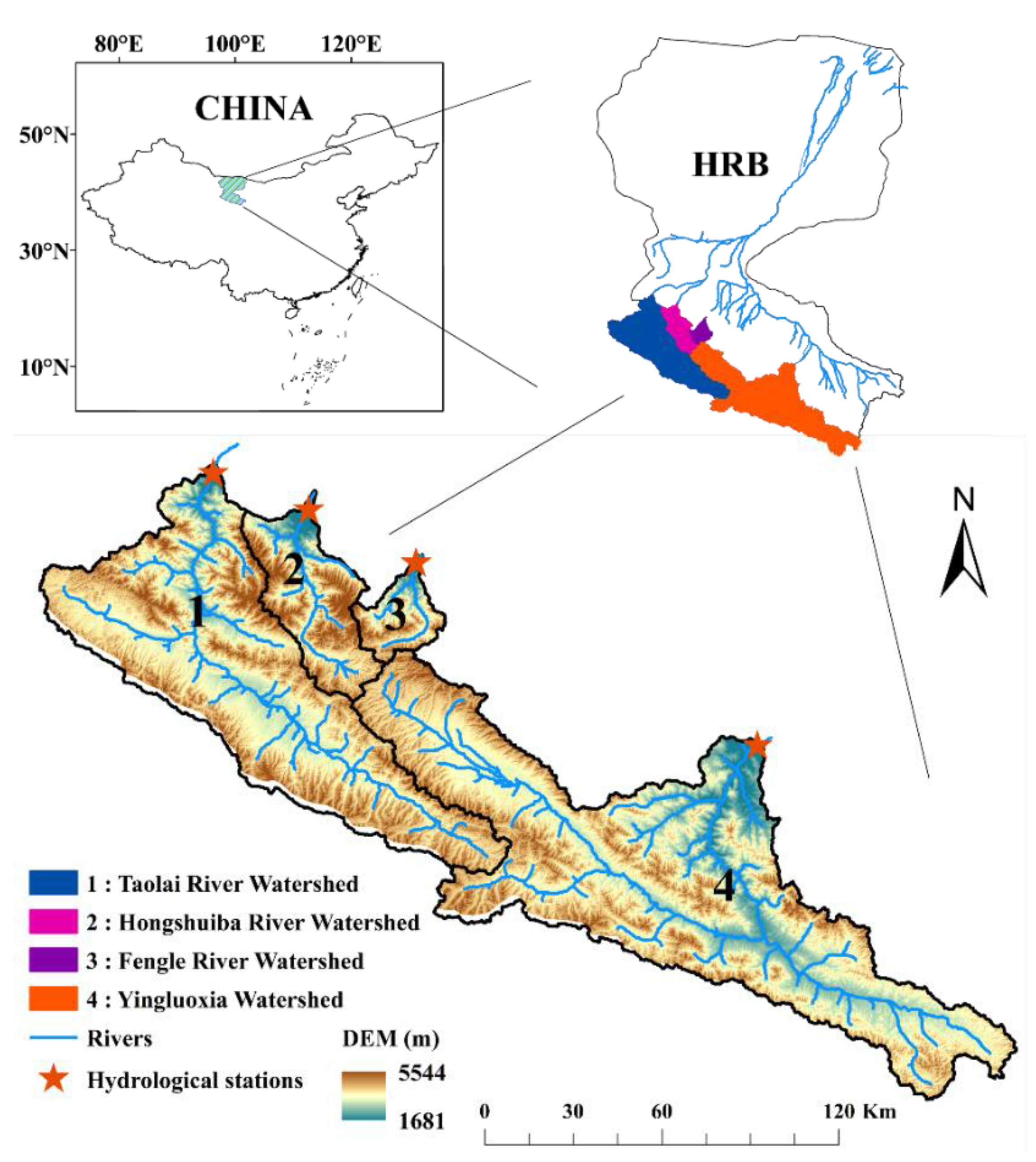
2.1. Study Area

The case study area (Figure 1) was located in the upstream region of the HRB (37.7°–42.7° N and 97.1°–102.0° E). The HRB is the second-largest endorheic river basin in northwestern China, covering an area of 128,900 km2. The main stream of the Heihe River is approximately 821 km long [28]. The upstream HRB consists of four neighboring watersheds, including the Fengle River Watershed (FRW), Hongshuiba River Watershed (HRW), Taolai River Watershed (TRW) and Yingluoxia Watershed (YW). The elevations of the four watersheds range from 1681 m to 5541 m. The areas of the FRW, HRW, TRW and YW are 574 km2, 1580 km2, 6924 km2 and 10,003 km2, respectively. The four watersheds lie on the northern margin of the Qilian Mountains, where the ecological system is characterized by snow cover, alpine meadows, evergreen needle-leaf forests and streamflow networks [29]. The rivers in the four watersheds are supplied by precipitation, glacier melting and groundwater discharge.

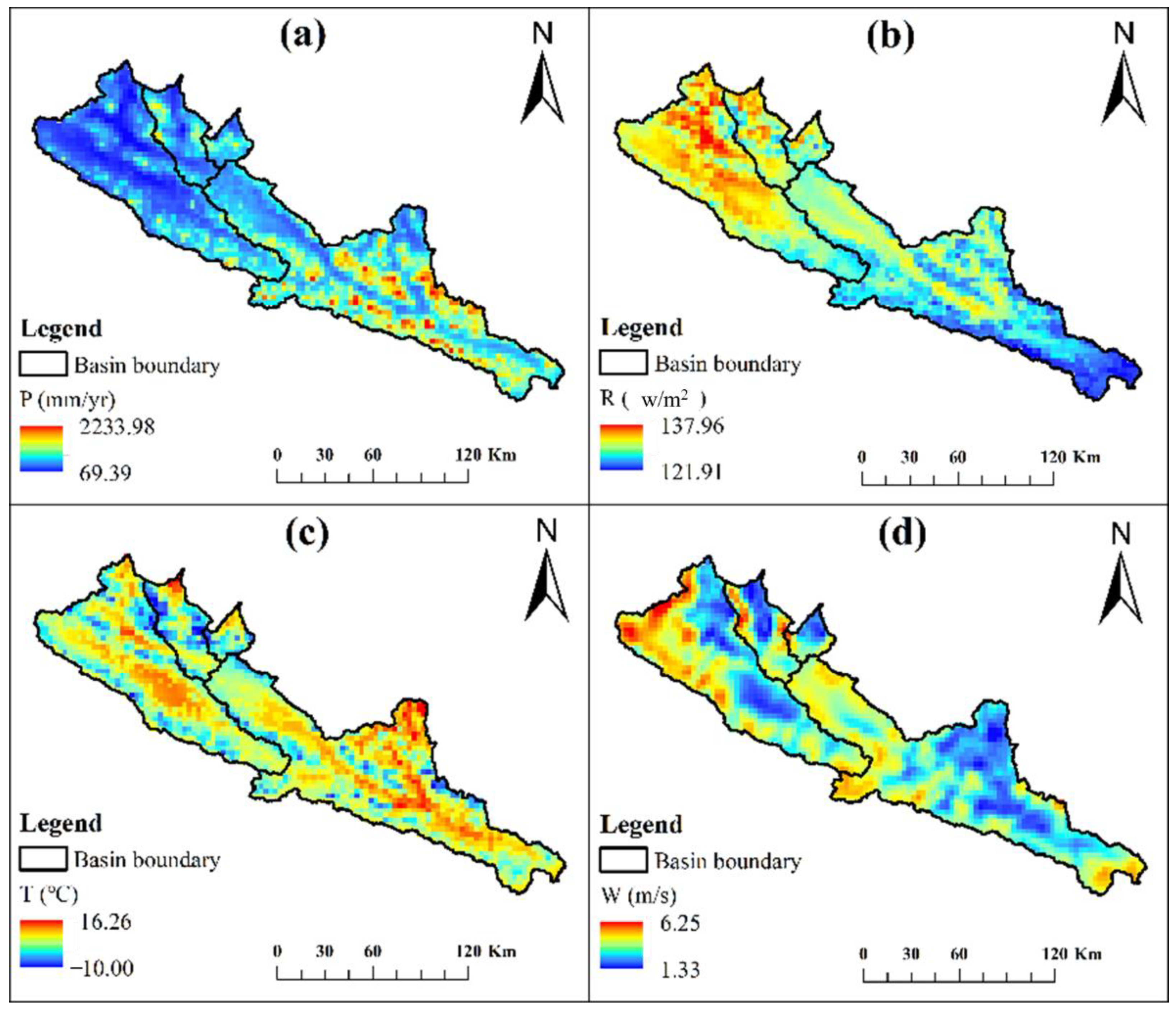
2.2. Data Description

The gridded climate datasets used in this study were produced using a climate model, i.e., the regional integrated environmental model system [30]. The datasets, as listed in Table 1, have a spatial resolution of 3 km × 3 km and a period spanning from 1 January 1990 to 31 December 2012. The number of grid points is 66 in the FRW, 177 in the HRW, 767 in the TRW and 1103 in the YW. The spatial distribution of the meteorological data in the study area is presented in Figure 1. The mean annual precipitation varies from 69.39 mm/yr to 2233.98 mm/yr, and high values are mainly distributed in the valley of the YW. The net solar radiation decreases from the northwest to the southeast. The temperature decreases with elevation, while the wind speed increases with elevation. Historical daily streamflow is monitored at the four gauging stations in the watershed outlets (Figure 2). In terms of the annual water volume, the first tier belongs to the YW, followed by the TRW, HRW and FRW. We split the timeframe of the data into 1990–2004 for the training period and 2005–2012 for the testing period.

3. Methodology

In this section, we first introduce the empirical orthogonal function (Section 3.1) and then describe the EOF, as well as the four ML models, namely, SVR, MLP, LSTM and GBRT (Section 3.2). Section 3.3 describes the main framework that involved integrating the ML models with EOF analysis. Section 3.4 illustrates the importance of different variables in the ML models. Some performance metrics are introduced in Section 3.5.

3.1. Empirical Orthogonal Function

EOF analysis, also known as principal components analysis (PCA), is regarded as a proper statistical approach for studying spatial patterns of climate variability and how they change with time. The principle of EOF analysis is to project a set of data onto a lower-dimensional space through linear transformation on the basis of maintaining significant information and discarding the interrelations of the original features. The new time series produced by the EOF algorithm are called principal components (PCs), which are uncorrelated with each other. The first PC retains the largest variance, the second PC has the second-largest variance, and so on. More information regarding EOF analysis can be found in [31].
Through EOF analysis, the climate data are individually transformed into several PCs. The explained variance ratio of the PCs corresponds to how much climate information the PCs can cover. It is of great importance to determine the number of PCs for each climate data set since fewer PCs mean less climate information but more PCs might result in useless noise. Equation (1) describes the explained variance ratio (EVR) of the first k PCs:
EVR = i = 1 k λ i i = 1 n λ i
where λ is the eigenvalue of the covariance matrix of the raw data, and n is the total number of eigenvalues. Usually, the EVR of the first k PCs needs to be more than 85% [32]. Therefore, this threshold value of 85% was accepted in this study.

3.2. Machine Learning Models

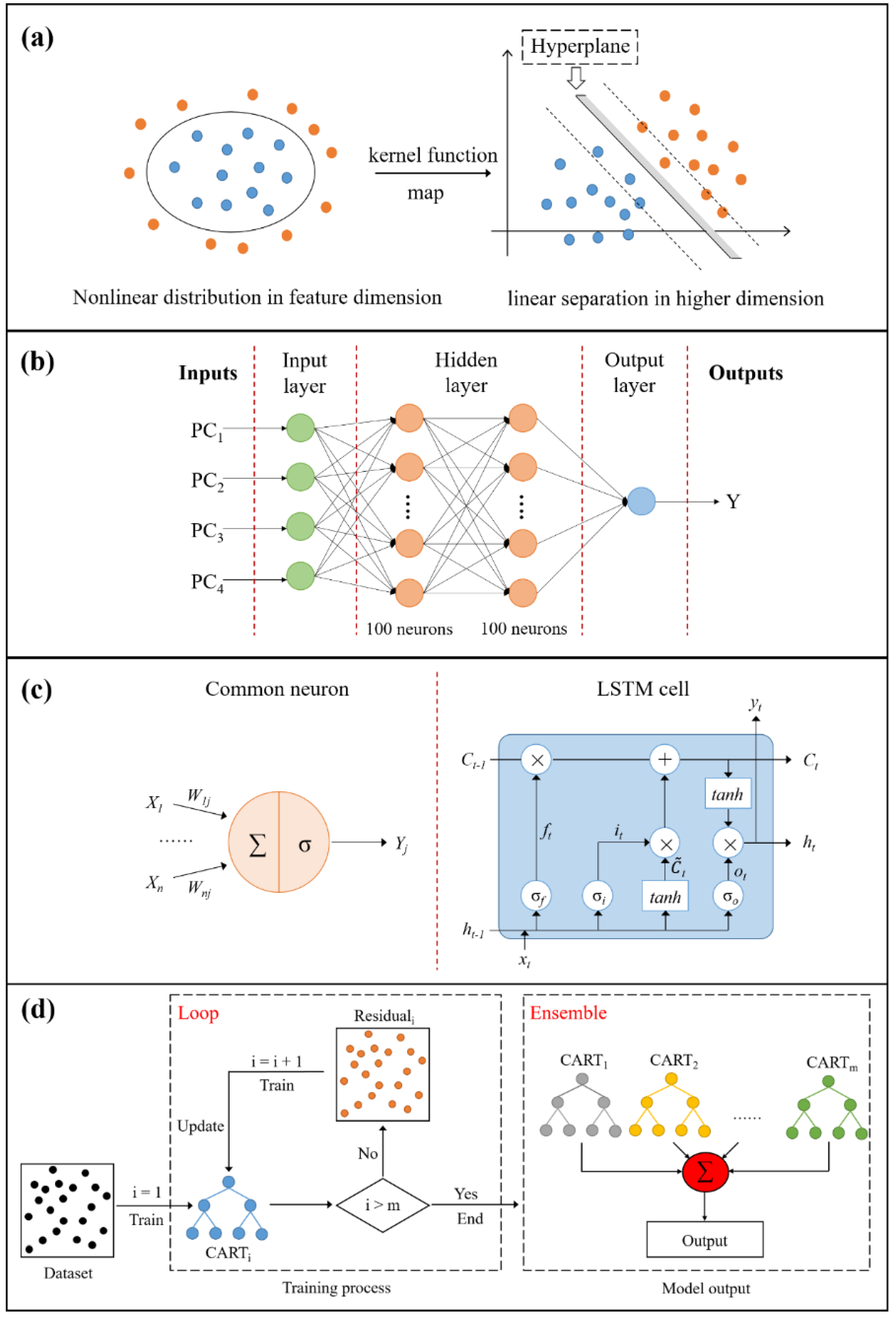
3.2.1. Support Vector Regression

The support vector machine (SVM), developed by Vapnik [33], is an ML model that is extensively used in classification and regression problems. SVR refers to a technique that applies the SVM to regression problems based on binary classification in the space of arbitrary properties [34], and it is able to map both linear and nonlinear relationships [35]. When the dataset is nonlinearly distributed in the feature space, the core of SVR is to use a kernel function to map the raw data into a higher dimensional space and then minimize the error to fully achieve regression efficiency [36] (Figure 3a). More details regarding SVR can be found in these studies [37,38]. The most widely used kernel function in SVR for hydrological studies is the radial basis function [39,40,41,42]. Dibike et al. further proposed that the radial basis function is the best kernel for a rainfall–runoff model [43]. We took the radial basis kernel, polynomial kernel and sigmoid kernel into consideration and determined that the radial basis function outperformed other kernel functions in this study.

3.2.2. Multilayer Perceptron

ANNs are designed to simulate the way biological neural systems analyze external signals and stimuli [44]. ANNs have many processing units (neurons) that are connected using weighted synaptic connections, such as a web [45]. This structure enables ANNs to reconstruct complex input–output relationships. In practice, the performance of an ANN model is greatly influenced by predefined hyperparameters, such as the network structure, activation function (transfer function) and training optimizer. Therefore, it is important for researchers to set up reliable hyperparameters before training ANN models.
The multilayer perceptron (MLP) model is one of the most frequently used ANNs in hydrologic modeling. In the MLP model, each neuron receives the input from the neurons in the preceding layer and renders the output as the input of the next layer. The connection weights of neurons upgrade as soon as the error signals flow backward. A detailed introduction to the MLP model is provided in [26]. Here, we employed a two-hidden-layer MLP model with one hundred neurons per hidden layer, in accordance with many experiments (in Figure 3b). The sigmoid function, hyperbolic tangent (tanh) function, rectified linear unit (ReLU) function and linear function are well-known among numerous activation functions. We compared these types of activation functions during hydrologic modeling and finally chose the sigmoid function for the hidden layer and the linear function for the output layer. The optimization function (optimizer) plays a pivotal role in updating the weights at each layer. Adam optimization is an adaptive learning rate method that is difficult to trap in the local optimum and feasible for computing sparse input datasets in high dimensions. Kingma and Ba demonstrated that Adam outperforms other stochastic optimization methods [46]. Hence, Adam was used to train our MLP model.

3.2.3. Long Short-Term Memory Network

LSTM is an advanced version of an RNN. Unlike an MLP, an RNN has special connections between nodes to form a cycle, making it exhibit temporal dynamics behavior. Classic RNNs have a simple cell where only one internal state variable exists; therefore, the ability to remember long-term sequences is limited. RNNs have difficulty learning long-duration sequential information because error signals across many time steps lead to vanishing gradients [47]. Designed by Graves et al. [48], LSTM can overcome the weakness of a traditional RNN by remembering the long-term state. LSTM has two cell states (referred to as c and h in Figure 3c) for information reservation and three types of gates to decide whether the information is lost or not [49]. As presented in Figure 3c, the first gate is called the forget gate (f), controlling which information will be discarded. The input gate (i) is the second gate, which is responsible for updating the cell state. The output gate (o), as the third gate, takes charge of what cell information flows into the next LSTM cell. More details regarding LSTM are presented in [15]. Similar to other types of ANNs, the LSTM network is also affected by hyperparameters. The LSTM model used in this study had two hidden layers with 100 cell units in Figure 3b because we found that a more complex structure hardly improved the prediction performance of the LSTM model. The activation function was the ReLU activation function at the hidden layer and the linear function at the output layer. Similar to the MLP model, the Adam optimizer was selected as the optimization algorithm.

3.2.4. Gradient Boosting Regression Tree

Ensemble learning assembles many base learners (weak learners) to enhance the capability of the base learner. Gradient boosting decision tree (GBDT), which is one of the most widely used ensemble learning methods, can serve as a classification model or a regression model in many modeling applications. GBRT (GBDT for regression) is composed of a set of base learners called CARTs. Initially introduced by Li et al. [50], a CART is a nonparametric algorithm using a binary tree for predicting continuous variables. The CART algorithm provides the best division of input space using nodes and obtains output values according to the inputs in the leaf nodes. The GBRT algorithm adopts the idea of gradient boosting to combine many CARTs to upgrade its regressive performance [18]. The GBRT formulation is depicted in Figure 3d, where m and i refer to the maximum number of CARTs and the ith CART, respectively. The first CART is trained by the original dataset and the next CART is trained by the residual of the last CART. The loop ends as soon as i exceeds m. Eventually, the GBRT model outputs the sum of all CARTs.
The structure of the GBRT model (e.g., the maximum depth and the number of CARTs) can significantly influence the models’ forecasting capabilities. Based on a set of scenario analyses for various combinations of model structures, the number of CARTs was set to 300, and the maximum depth of each CART was set to 5. The loss function also influences the performance of the GBRT model. The quantile loss becomes an evaluation model of GBRT other than the mean square loss, taking into account the fact that the quantile loss is suitable for many outliers.

3.3. Integration of the EOF and ML Models

We integrated four ML models with the EOF to simulate streamflow for the four selected watersheds. As shown in Figure 4, the general framework of the ML model with the EOF includes several necessary preprocessing procedures (blue arrow lines) and rainfall–runoff modeling (red arrow lines). The aim of the preprocessing methods is to provide input data for the ML model. The process of rainfall–runoff modeling in practice is to minimize the loss function of the ML models.
In the pre-process, the EOF technique was first utilized to process gridded climate data. Here, each type of climate data itself accepted EOF processing to obtain their PC series. The PC series of each climate dataset became an alternative to the gridded climate data. Then, the amount of PC series needed to be certified. This part is introduced in Section 4.1. The normalization method scaled the numerical value of the PC series to a range from zero to one. This normalization skill had a positive effect since it could accelerate the training process of the ML models. After normalization, four types of PCs were combined to build input vectors for the ML models. ML models used a one-week lag time, which meant model inputs were PCs of the latest seven days. The streamflow also accepted a zero–one scaler for normalization and then compared it with the output of the ML models.
In rainfall–runoff modeling, the four types of ML models mentioned above were trained to build the optimal simulation model individually. The SVR library and GBRT library were both Scikit-learn modules. The MLP library and LSTM library were TensorFlow and Keras. The library where we carried out the EOF processing and normalization was the Scikit-learn module [51].
To investigate the effect of employing EOF analysis in streamflow prediction, the EOF preprocessing method was compared with a simple arithmetic preprocessing method. In this arithmetic method, the climate predictors of the streamflow were the sum of gridded P and gridded R and the average of gridded T and gridded W. This method simply interpreted the hydrometeorological factors of streamflow within a watershed.

3.4. Variable Importance Analysis in ML Models

The ML models in this study built numerical mappings of climate predictors and streamflow targets. For well-trained ML rainfall–runoff models, all climate data contribute to the predicted streamflow to some degree. Here, we explored how the ML models used these climate data to simulate the streamflow through a simple variable importance analysis.
A streamflow series was simulated using well-trained ML models. The input framework of the ML models included four types of climate PC series. Then, we created a new input framework that excluded one climate PC series (numerical value becomes zero) and kept the other three climate PC series unchanged. A new streamflow series was simulated by feeding a new input framework into the well-trained ML models. The difference between the two streamflow series was regarded as the quantitative influence of this climate predictor on the streamflow simulated by the well-trained ML models. Finally, to obtain a better observation, the difference needed to be divided by the old streamflow series. For example, the contribution of the variable P, denoted by C P , could be represented as follows (Equation (2)):
C P = 1 ML ( Φ ) ML ( P ,   Φ )
where Φ denotes other variables except P in the machine learning model ML.

3.5. Performance Measurements

Four performance measurements were adopted to calibrate the model parameters and evaluate the ML forecasting accuracies, namely, the root-mean-square error (RMSE), mean absolute error (MAE), Nash–Sutcliffe efficiency (NSE) coefficient and percent bias (Pbias). These measurements are commonly recommended for analyzing the forecasting reliability of hydrological models [52,53]. Both the RMSE and MAE act as references that straightforwardly convey the error between the observations and predictions in the regression model. The NSE is identified as one of the best hydrological metrics for determining the fitting performance of hydrology models [54]. The NSE value ranges between negative infinity and one. Value one means an ideal fitting for one model, while a score less than zero indicates that the hydrological model is unacceptable. Pbias can serve as a threshold that measures whether the total simulations are larger or less than their observations.
RMSE = 1 N i = 1 N ( y i o b s y i s i m ) 2
MAE = 1 N i = 1 N | ( y i o b s y i s i m ) |
NSE = 1 i = 1 N ( y i o b s y i s i m ) 2 i = 1 N ( y i o b s y o b s ¯ ) 2  
Pbias = i = 1 N ( y i s i m y i o b s ) i = 1 N y i o b s 100 %    
where y i o b s and y i s i m are the observed and predicted values, respectively, and y o b s ¯ is the arithmetical mean of the observed values.

4. Results and Discussion

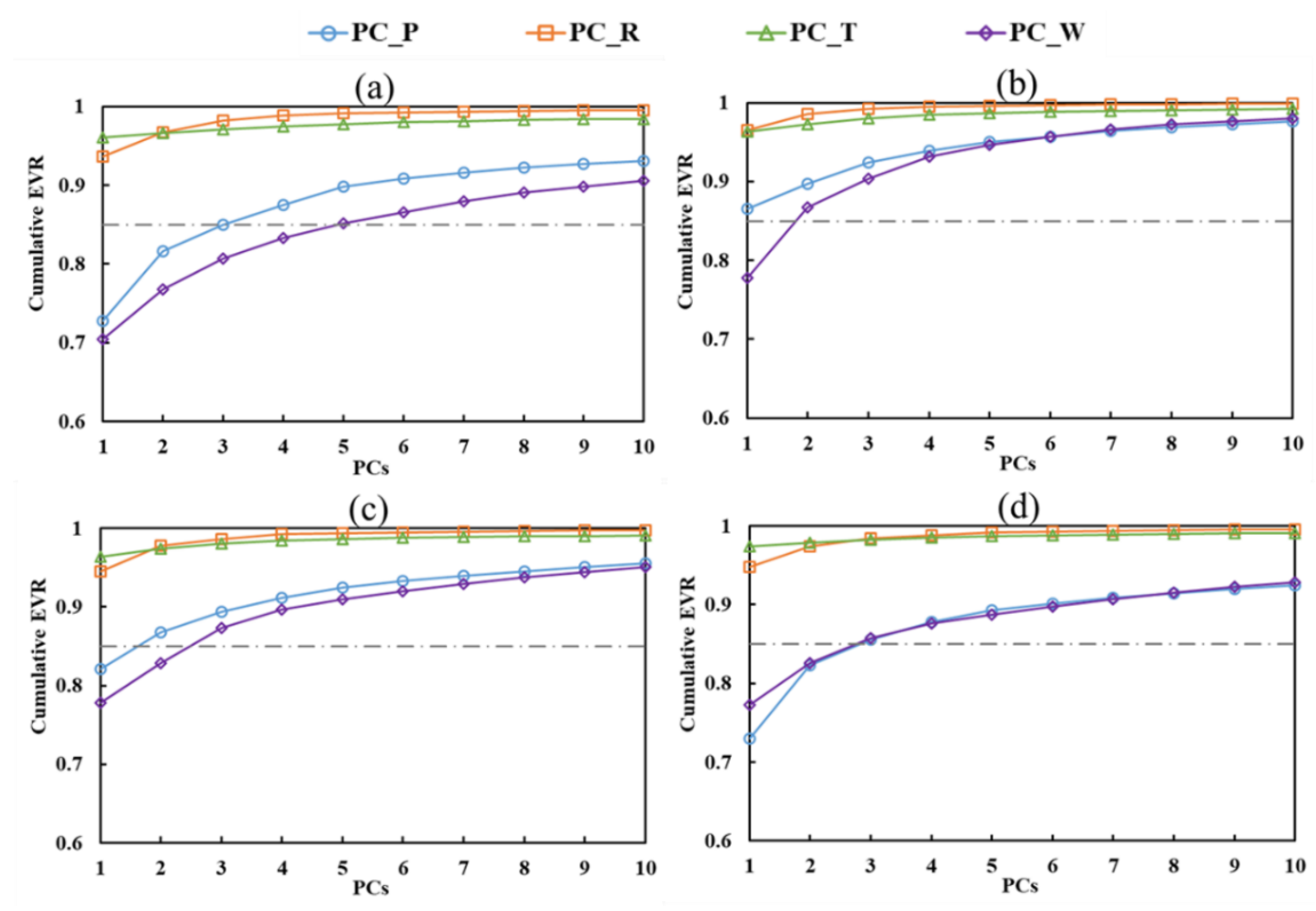
4.1. Selection of Reliable Predictors

Figure 5 presents the cumulative EVR of the first ten PCs for each climate variable in the four watersheds. The first PC_P, PC_R, PC_T and PC_W clearly explained more than 70% of the variance in their original data for the four watersheds, and even the first PC_R and PC_T accounted for up to 90%. This result illustrated that there was a strong correlation in every gridded climate dataset. Table 2 displays the number of grid points for the four watersheds and the number of selected PCs for each climate dataset. These selected PCs were substitutes for the gridded climate data to form the predictors of the streamflow.

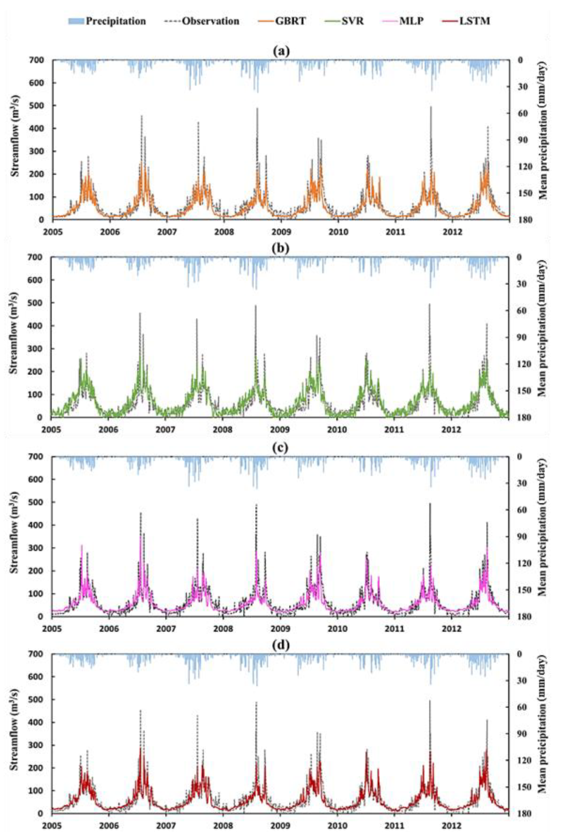
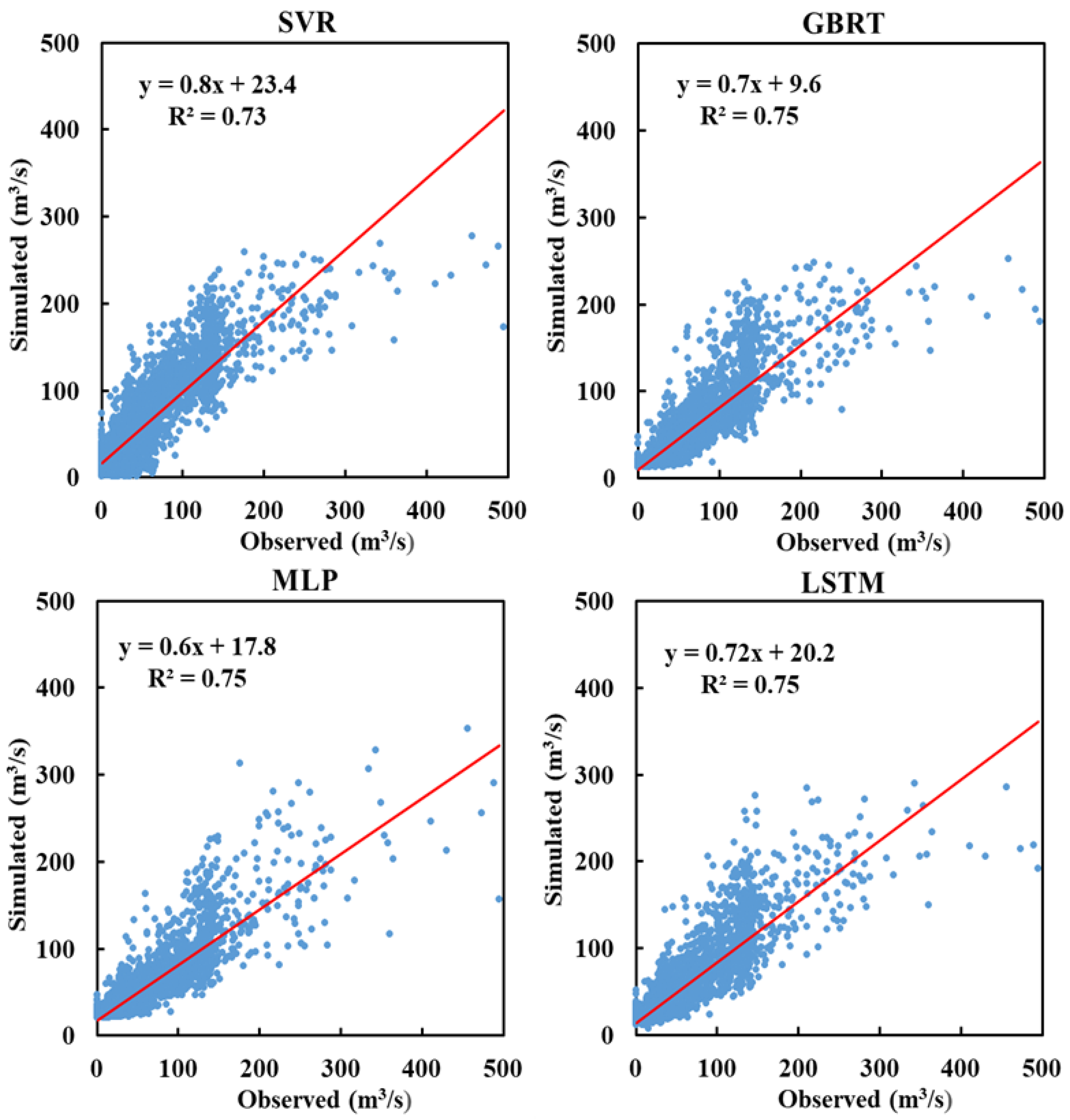
4.2. Comparison of ML Model Performance

Table 3 and Table 4 list the performance measurements of the four ML models in the training and testing periods. It was apparent that the GBRT model had the best performance among the four ML models for all watersheds during the training period (Table 3). During the testing period (Table 4), the GBRT model outperformed the other three models for the HRW and TRW, while LSTM had a better performance for the YW and FRW. As shown in Table 4, the best NSE value (the larger, the better) for each watershed was greater than 0.6 in the testing period. As recommended by Moriasi et al. [55], an NSE greater than 0.5 is regarded as acceptable statistics for a monthly estimation. It is well known that hydrological prediction for a daily resolution is more difficult than for a monthly resolution; thus, GBRT, MLP and LSTM were acceptable for daily streamflow prediction. As indicated by the Pbias values in Table 4, SVR overestimated the total water volume in each watershed, and the other three models underestimated the total water volume, especially the MLP model.
Figure 6 compares the observed and simulated hydrographs for the YW in the testing period. Figures S1–S3 in the Supplementary Materials show comparisons of the observed and simulated hydrographs for the FRW, HRW and TRW watersheds in the testing period, respectively. The four ML models could capture the daily temporal variations in the streamflow for the four watersheds. At a low flow value, GBRT, MLP and LSTM well matched the observations for the four watersheds, but SVR overestimated the streamflow for the FRW, HRW and TRW. All models seemed to underestimate the peak flow values, especially when predicting the largest streamflow in the FRW and HRW in the summer of 2010. However, the ML models showed different capabilities for predicting high flow. The MLP better matched the high flows than the other models for the YW (Figure 6), while GBRT better estimated the peak flows for the FRW (Figure S1), HRW (Figure S2) and TRW (Figure S3). As depicted in Figure 7 and Figure S4–S6, the best predicted results produced by the GBRT, MLP and LSTM models gave better linear regression lines than the SVM for all watersheds since the scatter diagrams of SVR showed the largest biases, lowest slope and lowest R2 values.
Overall, the GBRT model demonstrated the best potential for daily streamflow prediction, followed by LSTM, MLP and SVR. The GBRT models had the powerful capability of predicting the streamflow due to their base estimator (CART) and ensemble method (gradient boosting). On the one hand, CART is a robust model against outliers [50], with a flexible structure that quickly and correctly fits the target, even if there is noise in the training set. Furthermore, the nonparametric property of the CART model avoids setting complicated parametric functions, eliminating one of the sources of prediction error. On the other hand, the gradient boosted technique can improve the prediction accuracy of the base learner [56]. This sort of ensemble mode keeps the single weak learner relatively simple and optimizes the total residual from CARTs, protecting the GBRT models from overfitting. The LSTM models have a disadvantage in comparison with the GBRT models: the involvement of the model parameters and computation operations implies that LSTM easily converges to a local minimum. Once trapped in the local optima, LSTM might not yield satisfactory performance compared with GBR, such as in the HRW and FRW. Since the MLP network has a limited ability to deal with long time series tasks compared with LSTM, MLP performs worse than LSTM for streamflow prediction. It is difficult for SVR to solve all kinds of regression problems due to its rigid architecture. Despite the kernel function, the ability of SVR to deal with complex nonlinear regression is limited. Streamflow has a strong nonlinear dependence on meteorological factors; thus, it might be a difficult task for SVR to adequately capture all nonlinear responses of streamflow on meteorological driven forces.
Other studies also support our findings. For example, Erdal et al. pointed out that GBRT models produce better streamflow simulation results than other data-driven models, such as SVR and CART [19]; Ni et al. supposed that LSTM was more applicable than MLP for time series prediction [57], while Ghorbani et al. showed that MLP performed better than SVR for streamflow prediction in the Zarrinehrud River watershed [58].

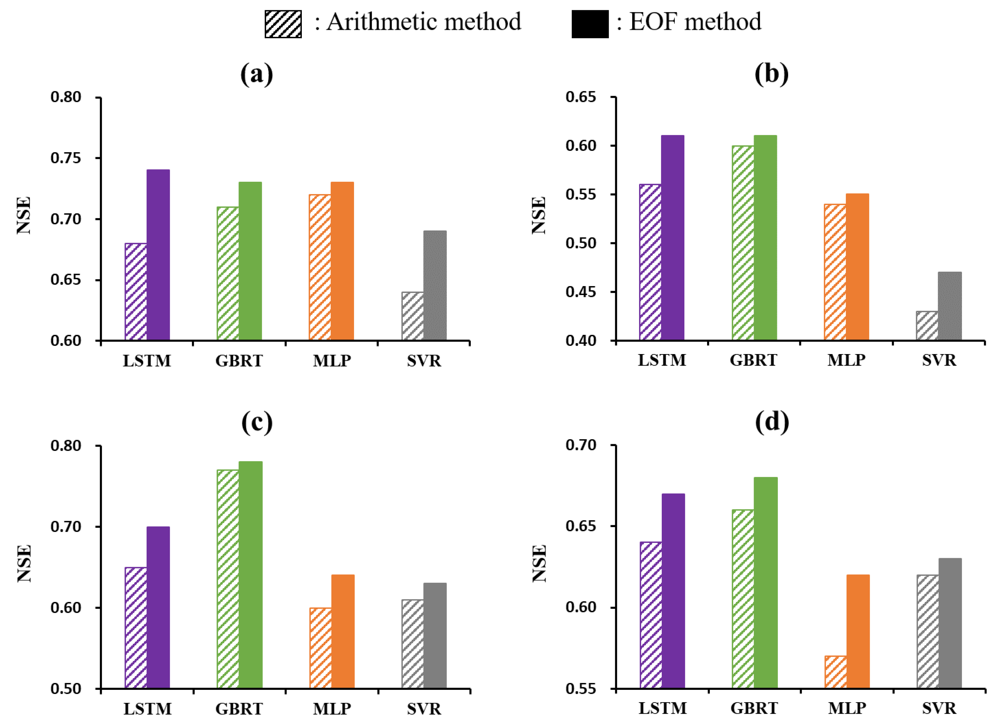
4.3. Role of EOF Analysis for Improving Streamflow Prediction

As shown in Figure 6, for the four watersheds, all ML models had higher NSE values when the PC series was used as a predictor of streamflow. Compared with the arithmetic method, EOF analysis increased the NSE by at least 0.02 (see Figure 8). The LSTM model exhibited more improvement than the other three models when coupled with EOF analysis. As expected, EOF analysis managed the gridded climate data better than the arithmetic method. An emphasis on the PC series concentrated on the first new PC, which accounted for most of the variance. The first PC was equal to the mean field of the gridded data. That is, the PC series contained not only the average gridded climate data but also other useful information about the gridded climate data. Thus, the EOF was better than the normal arithmetic method for drawing climate information from the gridded data.

4.4. Variable Importance in the Four ML Models

We used Equation (2) to illustrate the importance of precipitation in the four ML models. The result from Equation (2) represented the contribution of precipitation to streamflow predicted by the ML models. The contributions of the other three climate variables were determined in the same way. The results of the analysis in 2012 for the YW are depicted in Figure 9 for the LSTM model, Figure S7 for the GBRT model, Figure S8 for the MLP model and Figure S9 for the SVR model. We found that according to these diagrams, the climate contributions had nearly the same pattern in the SVR model, while for the LSTM, GBRT and MLP models, the contributions over time differed between the climate variables. Moreover, the results indicated that the LSTM model translated climate data into streamflow in a manner similar to the MLP model.
Data-driven ML models are always blamed for their “black-box” property due to the lack of hydrological interpretability. However, the LSTM model is a special ML model that is able to process long-term time series. Similar to traditional hydrological models, the LSTM output at every time step is influenced by the cell states that keep previous information. Kratzert et al. showed that the LSTM model does provide some hydrological interpretation due to the LSTM cells [15]. Thus, hydrological explanations of the climatic variables are revealed in the LSTM model. In our input–output framework, theoretically, precipitation (P) is positively correlated with streamflow, while net solar radiation (R), temperature (T) and wind speed (W) are negatively correlated with streamflow. For variable P, the contribution to streamflow in summer was higher than that in winter (in Figure 9a). This contribution corresponded to the natural law of precipitation in the YW for the whole year: more precipitation in summer contributed to more streamflow. For the variable R, the negative influence on streamflow in summer was greater than that in winner (in Figure 9b). The contribution graph of variable T looked a little interesting (in Figure 9c), i.e., unlike the variable R, there was less negative contribution in summer than in winter. This finding stemmed from the fact that snowmelt occurs in the YW when the temperature is over 0 °C. In summer, snowmelt streamflow offsets the ET contribution of the variable T, causing the negative contribution of the variable T to be lower. In Figure 9d, the streamflow contribution of the variable W nearly maintained a horizontal line. A larger wind speed may result in larger transpiration because an increased movement of the air around plants may result in a higher transpiration rate. The larger transpiration rate will result in smaller streamflow; therefore, wind speed exhibited a negative relationship with streamflow.
The above discusses the influence of climatic variability on streamflow. Additionally, streamflow variability also depends on watershed disturbance, such as forest disturbance and human activities [59,60]. In the upstream region of the HRB, over-grazing results in grassland degradation, which, in turn, alters the streamflow regime [61]. At present, the role of watershed disturbance on streamflow has not been thoughtfully investigated in the study area. It is necessary to consider watershed disturbance when simulating streamflow in future studies.

5. Conclusions

This study developed a general framework to improve streamflow forecasting by integrating ML models with EOF analysis. In the framework, EOF analysis was employed to pre-process the gridded climate data, and the ML models were used to build data-driven rainfall–runoff models. The framework enables the full use of gridded climate data that have rarely been used as the driving force for ML models. Currently, four popular ML models (i.e., SVM, GBRT, MLP and LSTM) are contained in the framework. As a case study, the framework was applied to simulate the streamflow for four sub-watersheds in the upper HRB, which is the second-largest endorheic river basin in China. The source code of the framework is available at https://github.com/DeepHydro/HydroML (accessed on 1 May 2022).
The major study findings were as follows. First, all four ML models were able to capture temporal variations in the streamflow and reproduce the hydrographs on a daily scale. However, different ML models exhibited different forecasting performances. GBRT outperformed the other three models, followed by LSTM, MLP and SVR. Second, the preprocessing of driving data by leveraging EOF improved the performance of the ML models. EOF analysis allowed us to extract the general pattern of the gridded climate data. The employment of EOF analysis caused the ML models to more efficiently learn the climate features in the gridded data. The introduction of the EOF analysis gave novel insight when the ML models used gridded data as the input series. Third, variable importance analysis revealed the contributions of climate predictors to the streamflow in the ML rainfall–runoff models. This analysis demonstrated that the LSTM model was a special ML model that provided hydrological explanations of each climate predictor.
The framework introduced in this study allowed for predicting streamflow only using climate data as driven forces. Thus, the framework can be used to predict future streamflows under different climate projections. In the past decade, how to improve the accuracy of long-term hydrological prediction using the iteratively multistep-ahead predictor approach has received much attention [62]. This study may provide a solution to this problem. However, it is important to note that the spatial variability of principal components (PCs obtained from EOF) in the current climate might be different in future climates.
This study still has a limitation that needs to be addressed in our future studies. A small underestimation of high flow occurred in the four ML models. The rainfall–runoff process is a complex hydrological process in a mountainous region. A simple model might not adequately simulate this behavior, as SVR does in this case. Inspired by the GBRT models, the multi-model ensemble technique might be a good choice. Araghinejad et al. successfully applied ensemble ANNs in rainfall-runoff modeling [63]. Moreover, considering that deep learning captures the nonlinear relationship in high-dimensional data, it is an intriguing topic to explore the potential of deep learning in streamflow forecasting. For instance, when performing the cross-correlation analysis between the climatic data and streamflow, we found that the climatic data in the next several days were correlated with the present streamflow. Bidirectional deep LSTM invented by Schuster and Paliwal can simultaneously convert the information to past (backward) and future (forward) states [64], which preserves the information in future meteorological data. Bidirectional deep LSTM shows a more powerful capacity than the LSTM, RNN and MLP models in other fields [65] but has not been employed in the application of hydrological events. The application of this model can further improve the performance of the rainfall–runoff model.

Supplementary Materials

The following supporting information can be downloaded at https://www.mdpi.com/article/10.3390/su14116612/s1. Figure S1: A comparison of observations and streamflow simulated by the (a) GBRT, (b) SVR, (c) MLP and (d) LSTM models in the FRW for the testing period. Figure S2: A comparison of observations and streamflow simulated by the (a) GBRT, (b) SVR, (c) MLP and (d) LSTM models in the HRW for the testing period. Figure S3: A comparison of observations and streamflow simulated by the (a) GBRT, (b) SVR, (c) MLP and (d) LSTM models in the TRW for the testing period. Figure S4: Scatter diagrams of daily streamflow observations and predictions from four types of ML models in the FRW for the testing period. Figure S5: Scatter diagrams of daily streamflow observations and predictions from four types of ML models in the HRW for the testing period. Figure S6: Scatter diagrams of daily streamflow observations and predictions from four types of ML models in the TRW for the testing period. Figure S7: Contribution of climatic elements to the daily streamflow in the GBRT model in 2012 for the YW: (a) contribution of P, (b) contribution of R, (c) contribution of T and (d) contribution of W. Figure S8: Contribution of climatic elements to the daily streamflow in the MLP model in 2012 for the YW: (a) contribution of P, (b) contribution of R, (c) contribution of T and (d) contribution of W. Figure S9: Contribution of climatic elements to the daily streamflow in the SVR model in 2012 for the YW: (a) contribution of P, (b) contribution of R, (c) contribution of T and (d) contribution of W.

Author Contributions

Conceptualization, Y.T.; methodology, Y.W. and Y.T.; validation, Y.C.; formal analysis, Y.W. and Y.T.; data curation, Y.W. and Y.C.; writing—original draft preparation, Y.W.; writing—review and editing, Y.W. and Y.C.; supervision, Y.T. All authors have read and agreed to the published version of the manuscript.

Funding

This research received funding from the National Natural Science Foundation of China (No. 42071244 and No. 41861124003) and the Strategic Priority Research Program of the Chinese Academy of Sciences (XDA20100104).

Institutional Review Board Statement

Not applicable.

Informed Consent Statement

Not applicable.

Data Availability Statement

Not applicable.

Acknowledgments

The authors are grateful for the support received by the National Natural Science Foundation of China and the Strategic Priority Research Program of the Chinese Academy of Sciences.

Conflicts of Interest

The authors declare no conflict of interest.

References

  1. Costabile, P.; Costanzo, C.; Macchione, F.; Mercogliano, P. Two-dimensional model for overland flow simulations: A case study. Eur. Water 2012, 38, 13–23. [Google Scholar]
  2. Tigkas, D.; Christelis, V.; Tsakiris, G. Comparative study of evolutionary algorithms for the automatic calibration of the Medbasin-D conceptual hydrological model. Environ. Process. 2016, 3, 629–644. [Google Scholar] [CrossRef]
  3. Liu, M.; Lu, J. Support vector machine―An alternative to artificial neuron network for water quality forecasting in an agricultural nonpoint source polluted river? Environ. Sci. Pollut. Res. 2014, 21, 11036–11053. [Google Scholar] [CrossRef]
  4. Singh, G.; Kandasamy, J.; Shon, H.; Cho, J. Measuring treatment effectiveness of urban wetland using hybrid water quality—artificial neural network (ANN) model. Desalin. Water Treat. 2011, 32, 284–290. [Google Scholar] [CrossRef]
  5. Mohanty, S.; Jha, M.K.; Kumar, A.; Panda, D. Comparative evaluation of numerical model and artificial neural network for simulating groundwater flow in Kathajodi―Surua Inter-basin of Odisha, India. J. Hydrol. 2013, 495, 38–51. [Google Scholar] [CrossRef]
  6. Yoon, H.; Jun, S.-C.; Hyun, Y.; Bae, G.-O.; Lee, K.-K. A comparative study of artificial neural networks and support vector machines for predicting groundwater levels in a coastal aquifer. J. Hydrol. 2011, 396, 128–138. [Google Scholar] [CrossRef]
  7. Kisi, O.; Choubin, B.; Deo, R.C.; Yaseen, Z.M. Incorporating synoptic-scale climate signals for streamflow modelling over the Mediterranean region using machine learning models. Hydrol. Sci. J. 2019, 64, 1240–1252. [Google Scholar] [CrossRef]
  8. Parisouj, P.; Mohebzadeh, H.; Lee, T. Employing machine learning algorithms for streamflow prediction: A case study of four river basins with different climatic zones in the United States. Water Resour. Manag. 2020, 34, 4113–4131. [Google Scholar] [CrossRef]
  9. Adnan, R.M.; Liang, Z.; Heddam, S.; Zounemat-Kermani, M.; Kisi, O.; Li, B. Least square support vector machine and multivariate adaptive regression splines for streamflow prediction in mountainous basin using hydro-meteorological data as inputs. J. Hydrol. 2020, 586, 124371. [Google Scholar] [CrossRef]
  10. Lin, J.-Y.; Cheng, C.-T.; Chau, K.-W. Using support vector machines for long-term discharge prediction. Hydrol. Sci. J. 2006, 51, 599–612. [Google Scholar] [CrossRef]
  11. Guo-rong, Y.; Zi-qiang, X. Prediction model of chaotic time series based on support vector machine and its application to runoff. Adv. Water Sci. 2008, 19, 116–122. [Google Scholar]
  12. Dolling, O.R.; Varas, E.A. Artificial neural networks for streamflow prediction. J. Hydraul. Res. 2002, 40, 547–554. [Google Scholar] [CrossRef]
  13. Jiang, S.; Zheng, Y.; Babovic, V.; Tian, Y.; Han, F. A computer vision-based approach to fusing spatiotemporal data for hydrological modeling. J. Hydrol. 2018, 567, 25–40. [Google Scholar] [CrossRef]
  14. Greff, K.; Srivastava, R.K.; Koutník, J.; Steunebrink, B.R.; Schmidhuber, J. LSTM: A search space odyssey. IEEE Trans. Neural Netw. Learn. Syst. 2016, 28, 2222–2232. [Google Scholar] [CrossRef] [PubMed] [Green Version]
  15. Kratzert, F.; Klotz, D.; Brenner, C.; Schulz, K.; Herrnegger, M. Rainfall-runoff modelling using long short-term memory (LSTM) networks. Hydrol. Earth Syst. Sci. 2018, 22, 6005–6022. [Google Scholar] [CrossRef] [Green Version]
  16. Zhang, J.; Zhu, Y.; Zhang, X.; Ye, M.; Yang, J. Developing a Long Short-Term Memory (LSTM) based model for predicting water table depth in agricultural areas. J. Hydrol. 2018, 561, 918–929. [Google Scholar] [CrossRef]
  17. Hancock, T.; Put, R.; Coomans, D.; Vander Heyden, Y.; Everingham, Y. A performance comparison of modern statistical techniques for molecular descriptor selection and retention prediction in chromatographic QSRR studies. Chemom. Intell. Lab. Syst. 2005, 76, 185–196. [Google Scholar] [CrossRef]
  18. Friedman, J.H. Greedy function approximation: A gradient boosting machine. Ann. Stat. 2001, 29, 1189–1232. [Google Scholar] [CrossRef]
  19. Erdal, H.I.; Karakurt, O. Advancing monthly streamflow prediction accuracy of CART models using ensemble learning paradigms. J. Hydrol. 2013, 477, 119–128. [Google Scholar] [CrossRef]
  20. Zhang, L.; Yang, L.; Ma, T.; Shen, F.; Cai, Y.; Zhou, C. A self-training semi-supervised machine learning method for predictive mapping of soil classes with limited sample data. Geoderma 2021, 384, 114809. [Google Scholar] [CrossRef]
  21. Nativi, S.; Mazzetti, P.; Santoro, M.; Papeschi, F.; Craglia, M.; Ochiai, O. Big data challenges in building the global earth observation system of systems. Environ. Model. Softw. 2015, 68, 1–26. [Google Scholar] [CrossRef]
  22. Blankenau, P.A.; Kilic, A.; Allen, R. An evaluation of gridded weather data sets for the purpose of estimating reference evapotranspiration in the United States. Agric. Water Manag. 2020, 242, 106376. [Google Scholar] [CrossRef]
  23. Farrar, D.E.; Glauber, R.R. Multicollinearity in regression analysis: The problem revisited. Rev. Econ. Stat. 1967, 49, 92–107. [Google Scholar] [CrossRef]
  24. Bhattacharjya, R.K.; Chaurasia, S. Geomorphology based semi-distributed approach for modelling rainfall-runoff process. Water Resour. Manag. 2013, 27, 567–579. [Google Scholar] [CrossRef]
  25. Navarra, A.; Simoncini, V. A Guide to Empirical Orthogonal Functions for Climate Data Analysis; Springer: Dordrecht, The Netherlands, 2010; p. 151. [Google Scholar]
  26. Bienvenido-Huertas, D.; Rubio-Bellido, C.; Pérez-Ordóñez, J.L.; Moyano, J. Optimizing the evaluation of thermal transmittance with the thermometric method using multilayer perceptrons. Energy Build. 2019, 198, 395–411. [Google Scholar] [CrossRef]
  27. Hannachi, A.; Jolliffe, I.T.; Stephenson, D.B. Empirical orthogonal functions and related techniques in atmospheric science: A review. Int. J. Climatol. J. R. Meteorol. Soc. 2007, 27, 1119–1152. [Google Scholar] [CrossRef]
  28. Ma, M.; Frank, V. Interannual variability of vegetation cover in the Chinese Heihe River Basin and its relation to meteorological parameters. Int. J. Remote Sens. 2006, 27, 3473–3486. [Google Scholar] [CrossRef]
  29. Yao, Y.; Zhang, Y.; Liu, Q.; Liu, S.; Jia, K.; Zhang, X.; Xu, Z.; Xu, T.; Chen, J.; Fisher, J.B. Evaluation of a satellite-derived model parameterized by three soil moisture constraints to estimate terrestrial latent heat flux in the Heihe River basin of Northwest China. Sci. Total Environ. 2019, 695, 133787. [Google Scholar] [CrossRef]
  30. Xiong, Z.; Yan, X. Building a high-resolution regional climate model for the Heihe River Basin and simulating precipitation over this region. Chin. Sci. Bull. 2013, 58, 4670–4678. [Google Scholar] [CrossRef]
  31. Björnsson, H.; Venegas, S. A manual for EOF and SVD analyses of climatic data. CCGCR Rep. 1997, 97, 112–134. [Google Scholar]
  32. He, F.; Zhang, L. Prediction model of end-point phosphorus content in BOF steelmaking process based on PCA and BP neural network. J. Process Control 2018, 66, 51–58. [Google Scholar] [CrossRef]
  33. Vapnik, V. The Nature of Statistical Learning Theory; Springer Science & Business Media: Berlin/Heidelberg, Germany, 1999. [Google Scholar]
  34. Pai, P.F.; Hong, W.C. A recurrent support vector regression model in rainfall forecasting. Hydrol. Process. Int. J. 2007, 21, 819–827. [Google Scholar] [CrossRef]
  35. Yu, X.; Zhang, X.; Qin, H. A data-driven model based on Fourier transform and support vector regression for monthly reservoir inflow forecasting. J. Hydro-Environ. Res. 2018, 18, 12–24. [Google Scholar] [CrossRef]
  36. Cristianini, N.; Shawe-Taylor, J. An Introduction to Support Vector Machines and other Kernel-Based Learning Methods; Cambridge University Press: Cambridge, UK, 2000. [Google Scholar]
  37. Dhiman, H.S.; Deb, D.; Guerrero, J.M. Hybrid machine intelligent SVR variants for wind forecasting and ramp events. Renew. Sustain. Energy Rev. 2019, 108, 369–379. [Google Scholar] [CrossRef]
  38. García-Nieto, P.J.; García-Gonzalo, E.; Lasheras, F.S.; Fernández, J.A.; Muñiz, C.D. A hybrid DE optimized wavelet kernel SVR-based technique for algal atypical proliferation forecast in La Barca reservoir: A case study. J. Comput. Appl. Math. 2020, 366, 112417. [Google Scholar] [CrossRef]
  39. Behzad, M.; Asghari, K.; Eazi, M.; Palhang, M. Generalization performance of support vector machines and neural networks in runoff modeling. Expert Syst. Appl. 2009, 36, 7624–7629. [Google Scholar] [CrossRef]
  40. Li, P.H.; Kwon, H.H.; Sun, L.; Lall, U.; Kao, J.J. A modified support vector machine based prediction model on streamflow at the Shihmen Reservoir, Taiwan. Int. J. Clim. 2010, 30, 1256–1268. [Google Scholar] [CrossRef]
  41. Noori, R.; Karbassi, A.; Moghaddamnia, A.; Han, D.; Zokaei-Ashtiani, M.; Farokhnia, A.; Gousheh, M.G. Assessment of input variables determination on the SVM model performance using PCA, Gamma test, and forward selection techniques for monthly stream flow prediction. J. Hydrol. 2011, 401, 177–189. [Google Scholar] [CrossRef]
  42. Sivapragasam, C.; Liong, S.-Y. Flow categorization model for improving forecasting. Hydrol. Res. 2005, 36, 37–48. [Google Scholar] [CrossRef]
  43. Dibike, Y.B.; Velickov, S.; Solomatine, D.; Abbott, M.B. Model induction with support vector machines: Introduction and applications. J. Comput. Civ. Eng. 2001, 15, 208–216. [Google Scholar] [CrossRef]
  44. Haykin, S. Neural Networks: A Comprehensive Foundation, 2nd ed.; McMaster University Press: Hamilton, ON, Canada, 1999. [Google Scholar]
  45. Tiwari, M.K.; Chatterjee, C. Uncertainty assessment and ensemble flood forecasting using bootstrap based artificial neural networks (BANNs). J. Hydrol. 2010, 382, 20–33. [Google Scholar] [CrossRef]
  46. Da, K. A method for stochastic optimization. arXiv 2014, arXiv:1412.6980. [Google Scholar]
  47. Hochreiter, S.; Bengio, Y.; Frasconi, P.; Schmidhuber, J. Gradient flow in recurrent nets: The difficulty of learning long-term dependencies. In A Field Guide to Dynamical Recurent Neural Networks; Kremer, S.C., Kolen, J.F., Eds.; Wiley-IEEE Press: New York, NY, USA, 2001. [Google Scholar]
  48. Graves, A.; Mohamed, A.R.; Hinton, G. Speech Recognition with Deep Recurrent Neural Networks. In Proceedings of the 2013 IEEE International Conference on Acoustics, Speech and Signal Processing, Vancouver, BC, Canada, 26–31 May 2013; pp. 6645–6649. [Google Scholar]
  49. Hochreiter, S.; Schmidhuber, J. Long short-term memory. Neural. Comput. 1997, 9, 1735–1780. [Google Scholar] [CrossRef]
  50. Li, B.; Friedman, J.; Olshen, R.; Stone, C. Classification and regression trees (CART). Biometrics 1984, 40, 358–361. [Google Scholar]
  51. Pedregosa, F.; Varoquaux, G.; Gramfort, A.; Michel, V.; Thirion, B.; Grisel, O.; Blondel, M.; Prettenhofer, P.; Weiss, R.; Dubourg, V. Scikit-learn: Machine learning in Python. J. Mach. Learn. Res. 2011, 12, 2825–2830. [Google Scholar]
  52. Doycheva, K.; Horn, G.; Koch, C.; Schumann, A.; König, M. Assessment and weighting of meteorological ensemble forecast members based on supervised machine learning with application to runoff simulations and flood warning. Adv. Eng. Inf. 2017, 33, 427–439. [Google Scholar] [CrossRef] [Green Version]
  53. Patel, S.S.; Ramachandran, P. A comparison of machine learning techniques for modeling river flow time series: The case of upper Cauvery river basin. Water Resour. Manag. 2015, 29, 589–602. [Google Scholar] [CrossRef]
  54. Nash, J.E.; Sutcliffe, J.V. River flow forecasting through conceptual models part I—A discussion of principles. J. Hydrol. 1970, 10, 282–290. [Google Scholar] [CrossRef]
  55. Moriasi, D.N.; Arnold, J.G.; Van Liew, M.W.; Bingner, R.L.; Harmel, R.D.; Veith, T.L. Model evaluation guidelines for systematic quantification of accuracy in watershed simulations. Trans. ASABE 2007, 50, 885–900. [Google Scholar] [CrossRef]
  56. Belayneh, A.; Adamowski, J.; Khalil, B.; Quilty, J. Coupling machine learning methods with wavelet transforms and the bootstrap and boosting ensemble approaches for drought prediction. Atmos. Res. 2016, 172, 37–47. [Google Scholar] [CrossRef]
  57. Ni, L.; Wang, D.; Singh, V.P.; Wu, J.; Wang, Y.; Tao, Y.; Zhang, J. Streamflow and rainfall forecasting by two long short-term memory-based models. J. Hydrol. 2020, 583, 124296. [Google Scholar] [CrossRef]
  58. Ghorbani, M.A.; Zadeh, H.A.; Isazadeh, M.; Terzi, O. A comparative study of artificial neural network (MLP, RBF) and support vector machine models for river flow prediction. Environ. Earth Sci. 2016, 75, 476. [Google Scholar] [CrossRef]
  59. Hou, Y.; Zhang, M.; Liu, S.; Sun, P.; Yin, L.; Yang, T.; Wei, X. The hydrological impact of extreme weather-induced forest disturbances in a tropical experimental watershed in south China. Forests 2018, 9, 734. [Google Scholar] [CrossRef] [Green Version]
  60. Aryal, Y.; Zhu, J. Effect of watershed disturbance on seasonal hydrological drought: An improved double mass curve (IDMC) technique. J. Hydrol. 2020, 585, 124746. [Google Scholar] [CrossRef]
  61. Qi, S.; Cai, Y. Mapping and Assessment of Degraded Land in the Heihe River Basin, Arid Northwestern China. Sensors 2007, 7, 2565–2578. [Google Scholar] [CrossRef] [Green Version]
  62. Yang, J.S.; Yu, S.P.; Liu, G.M. Multi-step-ahead predictor design for effective longterm forecast of hydrological signals using a novel wavelet neural network hybrid model. Hydrol. Earth Syst. Sci. 2013, 17, 4981–4993. [Google Scholar] [CrossRef] [Green Version]
  63. Araghinejad, S.; Azmi, M.; Kholghi, M. Application of artificial neural network ensembles in probabilistic hydrological forecasting. J. Hydrol. 2011, 407, 94–104. [Google Scholar] [CrossRef]
  64. Schuster, M.; Paliwal, K.K. Bidirectional recurrent neural networks. IEEE Trans. Signal Process. 1997, 45, 2673–2681. [Google Scholar] [CrossRef] [Green Version]
  65. Graves, A.; Schmidhuber, J. Framewise phoneme classification with bidirectional LSTM and other neural network architectures. Neural. Netw. 2005, 18, 602–610. [Google Scholar] [CrossRef]
Figure 1. The study area. The two top maps show the location of the study area in China. Four selected watersheds in the upper HRB are marked with different colors. The bottom map is a DEM map with hydrological stations and stream networks.
Sustainability 14 06612 g001
Figure 2. The spatial heterogeneity of the four hydrometeorological data in the study area: (a) mean annual precipitation, (b) mean daily net solar radiation, (c) mean daily temperature and (d) mean daily wind speed.
Sustainability 14 06612 g002
Figure 3. Schematic diagrams of the four selected ML models: (a) the importance of the kernel function in the SVR model, (b) the structure of the MLP and LSTM models used in this study, (c) the difference between neurons and LSTM cells, and (d) the principle of the GBRT.
Sustainability 14 06612 g003
Figure 4. The framework of the ML models with EOF analysis.
Sustainability 14 06612 g004
Figure 5. Cumulative explained variance ratio (cumulative EVR) of the PCs for the four climatic datasets in (a) YW, (b) FRW, (c) HRW and (d) TRW. The grey dotted line refers to the threshold of 85%. PC_P, PC_R, PC_T and PC_W represent the PCs of the precipitation, net solar radiation, temperature and wind speed, respectively.
Sustainability 14 06612 g005
Figure 6. A comparison of the observations and streamflows simulated using (a) GBRT, (b) SVR, (c) MLP and (d) LSTM in the YW for the testing period.
Sustainability 14 06612 g006
Figure 7. Scatter diagrams of the observed and predicted daily streamflows used by four types of ML models in the YW for the testing period.
Sustainability 14 06612 g007
Figure 8. Comparison of model performance between the arithmetic method and EOF analysis for building streamflow prediction models in the (a) YW, (b) FRW, (c) HRW and (d) TRW.
Sustainability 14 06612 g008
Figure 9. Contribution of climatic elements to the daily streamflow in the LSTM model in 2012 for the YW: (a) contribution of P, (b) contribution of R, (c) contribution of T and (d) contribution of W.
Sustainability 14 06612 g009
Table 1. Multisource variables for the data-driven models: P (precipitation), R (net solar radiation), T (surface temperature), W (wind speed) and Q (streamflow).
CategoryVariable (Unit)Spatial ResolutionTimeframeFile Format
PredictorsP (mm)3 km × 3 km1990–2012 (daily)NetCDF file
R (W/m2)3 km × 3 km1990–2012 (daily)NetCDF file
T (°C)3 km × 3 km1990–2012 (daily)NetCDF file
W (m/s)3 km × 3 km1990–2012 (daily)NetCDF file
ResponsesQ (m3/s)4 stations1990–2012 (daily)Excel file
Table 2. The number of selected PCs for the four watersheds.
WatershedDataGrid PointsNumber of PCsCumulative EVR
YWP1103487.5%
R1103193.7%
T1103196.0%
W1103585.2%
FRWP66186.6%
R66196.5%
T66196.3%
W66286.7%
HRWP177286.8%
R177194.5%
T177196.4%
W177387.3%
TRWP767385.5%
R767194.8%
T767197.4%
W767385.8%
Note: Variables P, R, T and W refer to the precipitation, net solar radiation, temperature and wind speed, respectively.
Table 3. Daily performances of the four ML models in the four watersheds for the training period.
WatershedsMetricsModels
SVRGBRTMLPLSTM
YWRMSE34.9121.8129.9430.69
MAE24.478.3517.6419.72
NSE0.570.830.680.66
Pbias0.27−0.020.050.18
FRWRMSE3.431.642.732.45
MAE2.450.571.361.13
NSE0.520.890.700.76
Pbias0.45−0.02−0.160.03
HRWRMSE8.595.377.616.86
MAE6.222.003.132.88
NSE0.590.840.680.74
Pbias0.44−0.04−0.14−0.10
TRWRMSE10.454.648.548.28
MAE6.511.934.103.97
NSE0.500.900.670.69
Pbias0.17−0.01−0.10−0.07
Note: The bold numbers indicate the best model performance.
Table 4. Daily performances of the four ML models in the selected watersheds for the testing period.
WatershedsMetricModels
SVRGBRTMLPLSTM
YWRMSE31.5729.7229.8728.92
MAE22.9718.7520.0419.82
NSE0.690.730.730.74
Pbias0.09−0.13−0.070.06
FRWRMSE4.483.854.113.82
MAE2.731.251.561.33
NSE0.470.600.550.62
Pbias0.42−0.10−0.22−0.05
HRWRMSE9.527.489.518.59
MAE6.633.414.243.90
NSE0.630.780.640.70
Pbias0.28−0.13−0.24−0.23
TRWRMSE10.309.4010.309.78
MAE6.545.185.525.59
NSE0.620.680.620.66
Pbias0.09−0.03−0.12−0.08
Note: The bold numbers indicate the best model performance.
Publisher’s Note: MDPI stays neutral with regard to jurisdictional claims in published maps and institutional affiliations.

