
Systematic Literature Review on Dynamic Life Cycle Inventory: Towards Industry 4.0 Applications

 ,
,  ,
,  and
and
Abstract
:1. Introduction
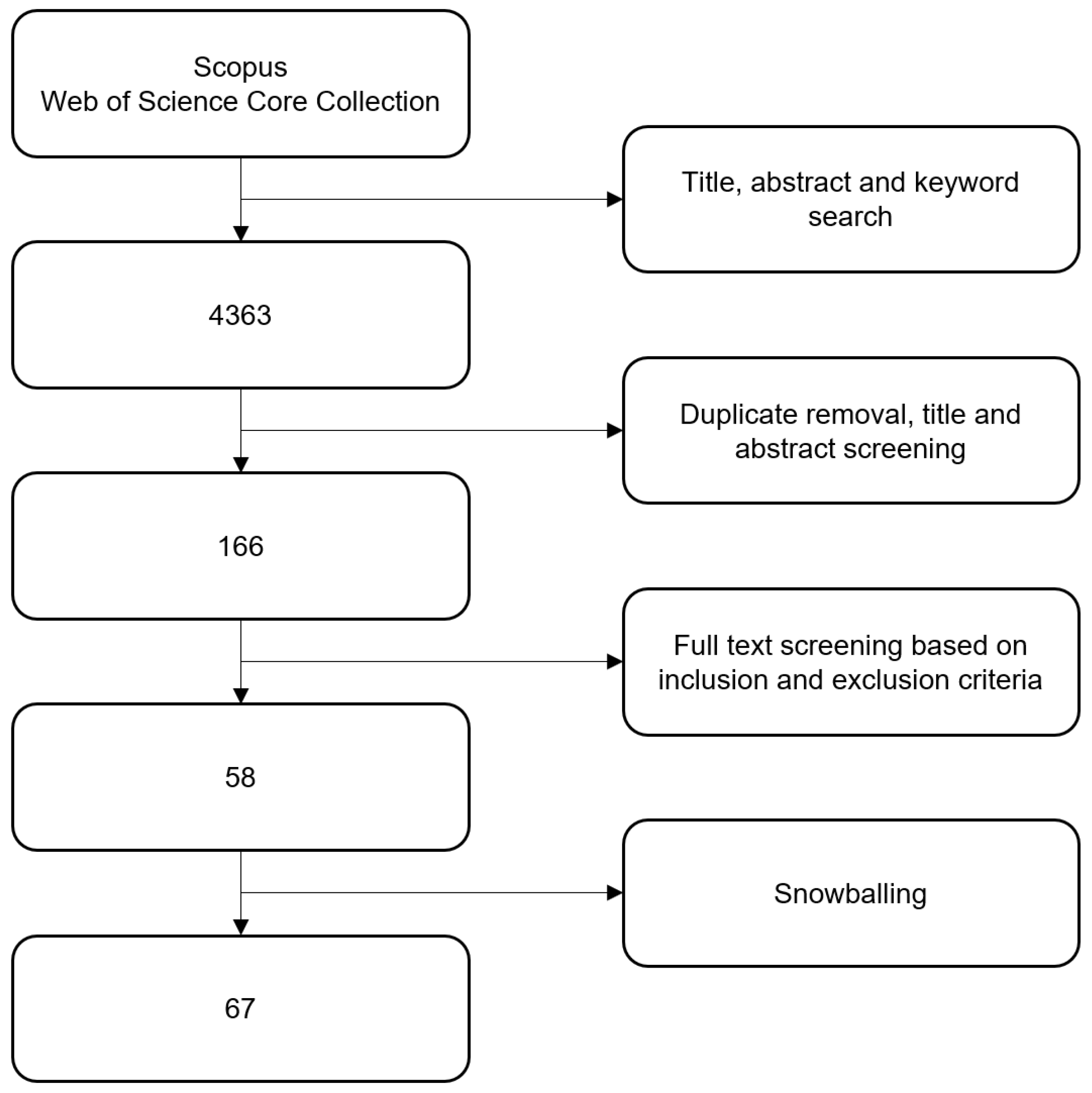
2. Methods
- question formulation;
- locating studies;
- study selection and evaluation;
- analysis and synthesis;
- reporting and using the results.
2.1. Question Formulation
- 1.
- What are the goals and scopes of the assessed studies?
- 2.
- How are existing methodologies able to integrate DLCI in LCA studies?
- 3.
- What are the characteristics of the proposed solutions and what are the opportunities for further development?
2.2. Locating Studies
2.3. Study Selection and Evaluation
2.4. Analysis and Synthesis
- Bibliographic information:
- -
- Title;
- -
- Authors;
- -
- Year of publication;
- -
- Journal;
- Goal and scope of the study:
- -
- Goal;
- -
- Type of the assessment: retrospective, scenario analysis, or forecast;
- -
- Static or continuous data collection;
- -
- Attributional or consequential modeling;
- Integration of dynamic LCI:
- -
- Modeling: white-box, gray-box, or black-box;
- -
- Dynamic component in the LCI;
- -
- Temporal resolution.
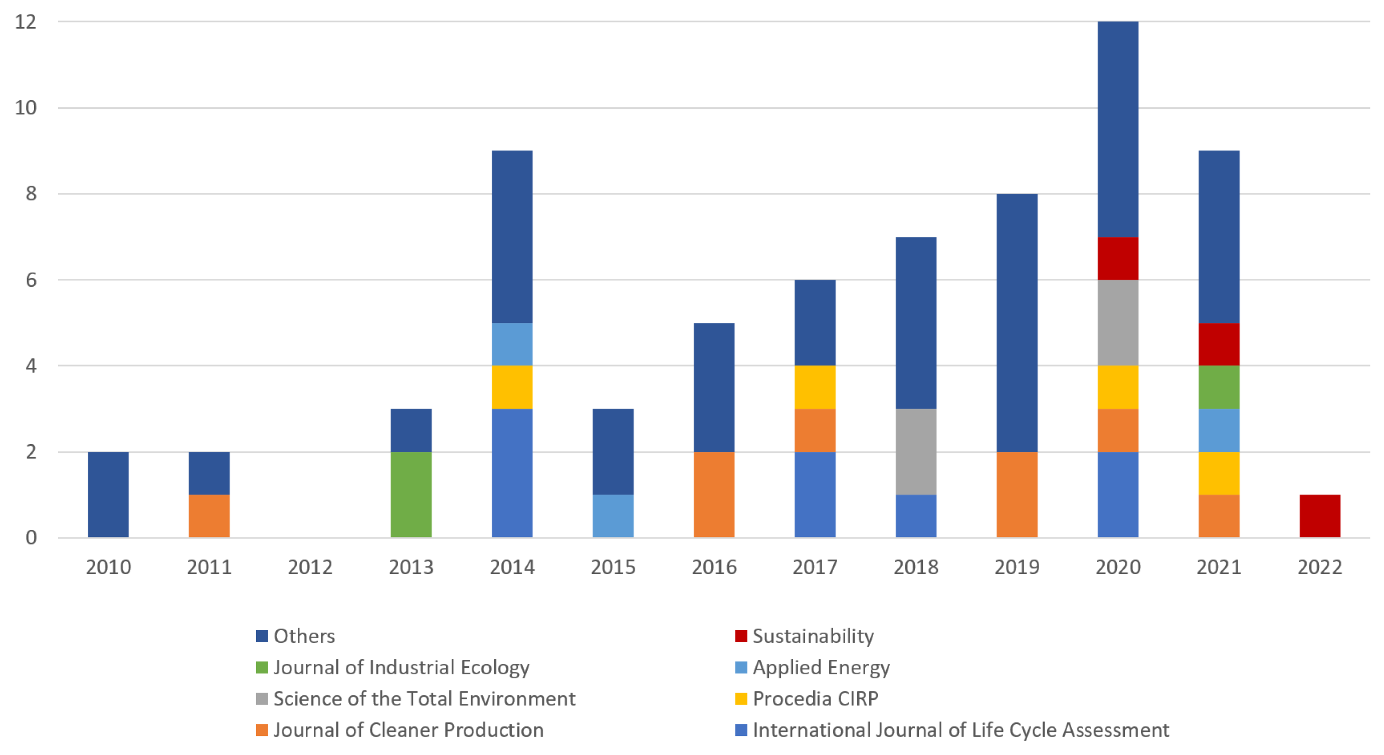
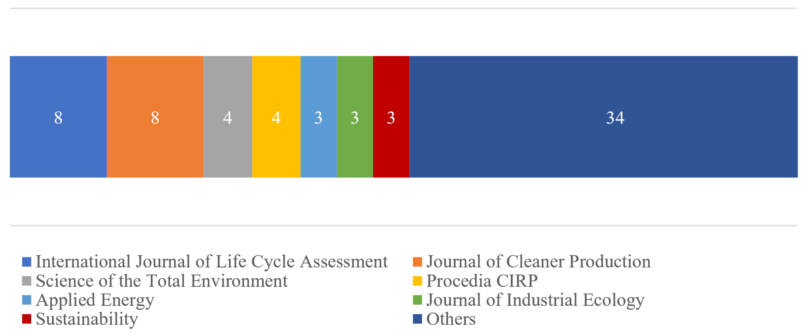
3. Results
3.1. Goal and Scope

| Type of Assessment | Previously Collected DLCI Data | Continuously Collected DLCI Data |
|---|---|---|
| Retrospective | [16,17,18,19,21,22,23,24,25,26,34,35,36,37,38,39,40,41,42,43,44,45,46,47,48,49,50] | [4,20,27,28,29,30,31,32,33,51] |
| Scenario analysis | [52,53,54,55,56,57,58,59,60,61,62,63,64,65,66,67,68,69] | [70,71,72] |
| Forecast | [73,74,75,76,77] |
3.2. Integration of Dynamic Life Cycle Inventory
3.3. Identification of Research Gaps
4. Discussion
5. Conclusions
Author Contributions
Funding
Institutional Review Board Statement
Conflicts of Interest
Abbreviations
| LCA | Life Cycle Assessment |
| LCI | Life Cycle Inventory |
| LCIA | Life Cycle Impact Assessment |
| DLCA | Dynamic Life Cycle Assessment |
| DLCI | Dynamic Life Cycle Inventory |
| CPS | Cyber-Physical System |
| DPI | Dynamic Process Inventory |
| DSys | Dynamic Systems Inventory |
| ESPA | Enhanced Structure Path Assessment |
| ERP | Enterprise Resource Planning |
| IoT | Internet-of-Things |
References
- ISO 14040; Environmental Management Life Cycle Assessment Principles and Framework. Technical Report; ISO: Geneva, Switzerland, 2006.
- ISO 14044; Environmental Management Life Cycle Assessment Requirements and Guidelines. Technical Report; ISO: Geneva, Switzerland, 2006.
- Bakas, I.; Hauschild, M.Z.; Astrup, T.F.; Rosenbaum, R.K. Preparing the ground for an operational handling of long-term emissions in LCA. Int. J. Life Cycle Assess. 2015, 20, 1444–1455. [Google Scholar] [CrossRef] [Green Version]
- Cerdas, F.; Thiede, S.; Juraschek, M.; Turetskyy, A.; Herrmann, C. Shop-floor Life Cycle Assessment. Procedia CIRP 2017, 61, 393–398. [Google Scholar] [CrossRef]
- Beloin-Saint-Pierre, D.; Albers, A.; Hélias, A.; Tiruta-Barna, L.; Fantke, P.; Levasseur, A.; Benetto, E.; Benoist, A.; Collet, P. Addressing temporal considerations in life cycle assessment. Sci. Total Environ. 2020, 743, 140700. [Google Scholar] [CrossRef] [PubMed]
- Kagermann, H.; Wahlster, W.; Helbig, J. Recommendations for Implementing the Strategic Initiative INDUSTRIE 4.0; Technical Report; Acatech: Munich, Germany, 2013. [Google Scholar]
- Dalenogare, L.S.; Benitez, G.B.; Ayala, N.F.; Frank, A.G. The expected contribution of Industry 4.0 technologies for industrial performance. Int. J. Prod. Econ. 2018, 204, 383–394. [Google Scholar] [CrossRef]
- Stock, T.; Seliger, G. Opportunities of Sustainable Manufacturing in Industry 4.0. Procedia CIRP 2016, 40, 536–541. [Google Scholar] [CrossRef] [Green Version]
- Bonilla, S.H.; Silva, H.R.; da Silva, M.T.; Gonçalves, R.F.; Sacomano, J.B. Industry 4.0 and sustainability implications: A scenario-based analysis of the impacts and challenges. Sustainability 2018, 10, 3740. [Google Scholar] [CrossRef] [Green Version]
- Thiede, S. Digital technologies, methods and tools towards sustainable manufacturing: Does Industry 4.0 support to reach environmental targets? Procedia CIRP 2021, 98, 1–6. [Google Scholar] [CrossRef]
- Chen, X.; Despeisse, M.; Johansson, B. Environmental sustainability of digitalization in manufacturing: A review. Sustainability 2020, 12, 298. [Google Scholar] [CrossRef]
- Sohn, J.; Kalbar, P.; Goldstein, B.; Birkved, M. Defining Temporally Dynamic Life Cycle Assessment: A Review. Integr. Environ. Assess. Manag. 2019, 16, 314–323. [Google Scholar] [CrossRef]
- Lueddeckens, S.; Saling, P.; Guenther, E. Temporal issues in life cycle assessment—A systematic review. Int. J. Life Cycle Assess. 2020, 25, 1385–1401. [Google Scholar] [CrossRef]
- Su, S.; Zhang, H.; Zuo, J.; Li, X.; Yuan, J. Assessment models and dynamic variables for dynamic life cycle assessment of buildings: A review. Environ. Sci. Pollut. Res. 2021, 28, 26199–26214. [Google Scholar] [CrossRef] [PubMed]
- Denyer, D.; Tranfield, D. Producing a Systematic Review. In The SAGE Handbook of Organizational Research Methods; Springer: Cham, Switzerland, 2009; pp. 671–689. [Google Scholar]
- Graff Zivin, J.S.; Kotchen, M.J.; Mansur, E.T. Spatial and temporal heterogeneity of marginal emissions: Implications for electric cars and other electricity-shifting policies. J. Econ. Behav. Organ. 2014, 107, 248–268. [Google Scholar] [CrossRef] [Green Version]
- Faria, R.; Marques, P.; Moura, P.; Freire, F.; Delgado, J.; De Almeida, A.T. Impact of the electricity mix and use profile in the life-cycle assessment of electric vehicles. Renew. Sustain. Energy Rev. 2013, 24, 271–287. [Google Scholar] [CrossRef]
- Rangaraju, S.; De Vroey, L.; Messagie, M.; Mertens, J.; Van Mierlo, J. Impacts of electricity mix, charging profile, and driving behavior on the emissions performance of battery electric vehicles: A Belgian case study. Appl. Energy 2015, 148, 496–505. [Google Scholar] [CrossRef]
- Messagie, M.; Mertens, J.; Oliveira, L.; Rangaraju, S.; Sanfelix, J.; Coosemans, T.; Van Mierlo, J.; Macharis, C. The hourly life cycle carbon footprint of electricity generation in Belgium, bringing a temporal resolution in life cycle assessment. Appl. Energy 2014, 134, 469–476. [Google Scholar] [CrossRef]
- Tao, F.; Zuo, Y.; Xu, L.D.; Lv, L.; Zhang, L. Internet of things and BOM-Based life cycle assessment of energy-saving and emission-reduction of products. IEEE Trans. Ind. Inf. 2014, 10, 1252–1261. [Google Scholar] [CrossRef]
- Brondi, C.; Cornago, S.; Piloni, D.; Brusaferri, A.; Ballarino, A. Application of LCA for the Short-Term Management of Electricity Consumption. In Life Cycle Assessment of Energy Systems and Sustainable Energy Technologies; Basosi, R., Cellura, M., Longo, S., Parisi, M., Eds.; Springer: Cham, Switzerland, 2019; Chapter 4; pp. 45–59. [Google Scholar] [CrossRef]
- Cardellini, G.; Mutel, C.L.; Vial, E.; Muys, B. Temporalis, a generic method and tool for dynamic Life Cycle Assessment. Sci. Total Environ. 2018, 645, 585–595. [Google Scholar] [CrossRef] [PubMed]
- Tiruta-Barna, L.; Pigné, Y.; Navarrete Gutiérrez, T.; Benetto, E. Framework and computational tool for the consideration of time dependency in Life Cycle Inventory: Proof of concept. J. Clean. Prod. 2016, 116, 198–206. [Google Scholar] [CrossRef]
- O’Connor, M.; Garnier, G.; Batchelor, W. Life cycle assessment of advanced industrial wastewater treatment within an urban environment. J. Ind. Ecol. 2013, 17, 712–721. [Google Scholar] [CrossRef]
- Roux, C.; Schalbart, P.; Peuportier, B. Accounting for temporal variation of electricity production and consumption in the LCA of an energy-efficient house. J. Clean. Prod. 2016, 113, 532–540. [Google Scholar] [CrossRef]
- Pigné, Y.; Gutiérrez, T.N.; Gibon, T.; Schaubroeck, T.; Popovici, E.; Shimako, A.H.; Benetto, E.; Tiruta-Barna, L. A tool to operationalize dynamic LCA, including time differentiation on the complete background database. Int. J. Life Cycle Assess. 2020, 25, 267–279. [Google Scholar] [CrossRef] [Green Version]
- Barni, A.; Fontana, A.; Menato, S.; Sorlini, M.; Canetta, L. Exploiting the Digital Twin in the Assessment and optimization of Sustainability Performances. In Proceedings of the 2018 International Conference on Intelligent Systems, Funchal, Portugal, 25–27 September 2018; pp. 706–713. [Google Scholar]
- Smolek, P.; Leobner, I.; Heinzl, B.; Gourlis, G.; Ponweiser, K. A method for real-time aggregation of a product footprint during manufacturing. J. Sustain. Dev. Energy Water Environ. Syst. 2016, 4, 360–378. [Google Scholar] [CrossRef] [Green Version]
- Jayapal, J.; Kumaraguru, S. Real-Time Linked Open Data for Life Cycle Inventory; Springer International Publishing: Berlin/Heidelberg, Germany, 2018; Volume 536, pp. 249–254. [Google Scholar] [CrossRef]
- Filleti, R.A.P.; Silva, D.A.L.; da Silva, E.J.; Ometto, A.R. Productive and environmental performance indicators analysis by a combined LCA hybrid model and real-time manufacturing process monitoring: A grinding unit process application. J. Clean. Prod. 2017, 161, 510–523. [Google Scholar] [CrossRef]
- Ferrari, A.M.; Volpi, L.; Settembre-Blundo, D.; García-Muiña, F.E. Dynamic life cycle assessment (LCA) integrating life cycle inventory (LCI) and Enterprise resource planning (ERP) in an industry 4.0 environment. J. Clean. Prod. 2021, 286. [Google Scholar] [CrossRef]
- Majanne, Y.; Korpela, T.; Judl, J.; Koskela, S.; Laukkanen, V.; Häyrinen, A. Real Time Monitoring of Environmental Efficiency of Power Plants. IFAC-PapersOnLine 2015, 48, 495–500. [Google Scholar] [CrossRef]
- Tu, M.; Chung, W.H.; Chiu, C.K.; Chung, W.; Tzeng, Y. A novel IoT-based dynamic carbon footprint approach to reducing uncertainties in carbon footprint assessment of a solar PV supply chain. In Proceedings of the 2017 4th International Conference on Industrial Engineering and Applications (ICIEA 2017), Nagoya, Japan, 21–23 April 2017; pp. 249–254. [Google Scholar] [CrossRef]
- Amor, M.B.; Gaudreault, C.; Pineau, P.O.; Samson, R. Implications of integrating electricity supply dynamics into life cycle assessment: A case study of renewable distributed generation. Renew. Energy 2014, 69, 410–419. [Google Scholar] [CrossRef] [Green Version]
- Beloin-Saint-Pierre, D.; Heijungs, R.; Blanc, I. The ESPA (Enhanced Structural Path Analysis) method: A solution to an implementation challenge for dynamic life cycle assessment studies. Int. J. Life Cycle Assess. 2014, 19, 861–871. [Google Scholar] [CrossRef] [Green Version]
- Collinge, W.O.; Rickenbacker, H.J.; Landis, A.E.; Thiel, C.L.; Bilec, M.M. Dynamic Life Cycle Assessments of a Conventional Green Building and a Net Zero Energy Building: Exploration of Static, Dynamic, Attributional, and Consequential Electricity Grid Models. Environ. Sci. Technol. 2018, 52, 11429–11438. [Google Scholar] [CrossRef]
- Di Florio, G.; Macchi, E.G.; Mongibello, L.; Baratto, M.C.; Basosi, R.; Busi, E.; Caliano, M.; Cigolotti, V.; Testi, M.; Trini, M. Comparative life cycle assessment of two different SOFC-based cogeneration systems with thermal energy storage integrated into a single-family house nanogrid. Appl. Energy 2021, 285, 116378. [Google Scholar] [CrossRef]
- Fagan, J.E.; Reuter, M.A.; Langford, K.J. Dynamic performance metrics to assess sustainability and cost effectiveness of integrated urban water systems. Resour. Conserv. Recycl. 2010, 54, 719–736. [Google Scholar] [CrossRef]
- Garcia, R.; Freire, F. Marginal life-cycle greenhouse gas emissions of electricity generation in Portugal and implications for electric vehicles. Resources 2016, 5, 41. [Google Scholar] [CrossRef]
- Groetsch, T.; Creighton, C.; Varley, R.; Kaluza, A.; Dér, A.; Cerdas, F.; Herrmann, C. A modular LCA/LCC-modelling concept for evaluating material and process innovations in carbon fibre manufacturing. Procedia CIRP 2021, 98, 529–534. [Google Scholar] [CrossRef]
- KC, R.; Aalto, M.; Korpinen, O.J.; Ranta, T.; Proskurina, S. Lifecycle Assessment of Biomass Supply Chain with the Assistance of Agent-Based Modelling. Sustainability 2020, 12, 1964. [Google Scholar] [CrossRef] [Green Version]
- Kono, J.; Ostermeyer, Y.; Wallbaum, H. The trends of hourly carbon emission factors in Germany and investigation on relevant consumption patterns for its application. Int. J. Life Cycle Assess. 2017, 22, 1493–1501. [Google Scholar] [CrossRef] [Green Version]
- Maurice, E.; Dandres, T.; Samson, R.; Moghaddam, R.F.; Nguyen, K.K.; Cheriet, M.; Lemieux, Y. Modelling of electricity mix in temporal differentiated life-cycle-assessment to minimize carbon footprint of a cloud computing service. In Proceedings of the 2014 Conference ICT for Sustainability, Stockholm, Sweden, 24–27 August 2014; pp. 290–298. [Google Scholar] [CrossRef] [Green Version]
- Munné-Collado, I.; Aprà, F.M.; Olivella-Rosell, P.; Villafáfila-Robles, R. The potential role of flexibility during peak hours on greenhouse gas emissions: A life cycle assessment of five targeted national electricity grid mixes. Energies 2019, 12, 4443. [Google Scholar] [CrossRef] [Green Version]
- Olindo, R.; Schmitt, N.; Vogtlander, J. Life Cycle Assessments on Battery Electric Vehicles and Electrolytic Hydrogen: The Need for Calculation Rules and Better Databases on Electricity. Sustainability 2021, 13, 5250. [Google Scholar] [CrossRef]
- Pinsonnault, A.; Lesage, P.; Levasseur, A.; Samson, R. Temporal differentiation of background systems in LCA: Relevance of adding temporal information in LCI databases. Int. J. Life Cycle Assess. 2014, 19, 1843–1853. [Google Scholar] [CrossRef]
- Ren, M.; Mitchell, C.R.; Mo, W. Managing residential solar photovoltaic-battery systems for grid and life cycle economic and environmental co-benefits under time-of-use rate design. Resour. Conserv. Recycl. 2021, 169, 105527. [Google Scholar] [CrossRef]
- Roux, C.; Schalbart, P.; Peuportier, B. Development of an electricity system model allowing dynamic and marginal approaches in LCA—Tested in the French context of space heating in buildings. Int. J. Life Cycle Assess. 2017, 22, 1177–1190. [Google Scholar] [CrossRef]
- Spatari, S.; Kandasamy, N.; Kusic, D.; Ellis, E.V. Energy and locational workload management in data centers. In Proceedings of the 2011 IEEE International Symposium on Sustainable Systems and Technology, Chicago, IL, USA, 16–18 May 2011; pp. 1–5. [Google Scholar] [CrossRef]
- Vuarnoz, D.; Jusselme, T. Temporal variations in the primary energy use and greenhouse gas emissions of electricity provided by the Swiss grid. Energy 2018, 161, 573–582. [Google Scholar] [CrossRef]
- Filleti, R.A.P.; Silva, D.A.L.; da Silva, E.J.; Ometto, A.R. Dynamic system for life cycle inventory and impact assessment of manufacturing processes. Procedia CIRP 2014, 15, 531–536. [Google Scholar] [CrossRef] [Green Version]
- Arvesen, A.; Völler, S.; Hung, C.R.; Krey, V.; Korpås, M.; Strømman, A.H. Emissions of electric vehicle charging in future scenarios: The effects of time of charging. J. Ind. Ecol. 2021, 25, 1250–1263. [Google Scholar] [CrossRef]
- Baumann, M.; Salzinger, M.; Remppis, S.; Schober, B.; Held, M.; Graf, R. Reducing the environmental impacts of electric vehicles and electricity supply: How hourly defined life cycle assessment and smart charging can contribute. World Electr. Veh. J. 2019, 10, 13. [Google Scholar] [CrossRef] [Green Version]
- Beloin-Saint-Pierre, D.; Padey, P.; Périsset, B.; Medici, V. Considering the dynamics of electricity demand and production for the environmental benchmark of Swiss residential buildings that exclusively use electricity. IOP Conf. Ser. Earth Environ. Sci. 2019, 323, 012096. [Google Scholar] [CrossRef]
- Collet, P.; Lardon, L.; Steyer, J.P.; Hélias, A. How to take time into account in the inventory step: A selective introduction based on sensitivity analysis. Int. J. Life Cycle Assess. 2014, 19, 320–330. [Google Scholar] [CrossRef]
- Elzein, H.; Dandres, T.; Levasseur, A.; Samson, R. How can an optimized life cycle assessment method help evaluate the use phase of energy storage systems? J. Clean. Prod. 2019, 209, 1624–1636. [Google Scholar] [CrossRef]
- Frossard, M.; Schalbart, P.; Peuportier, B. Dynamic and consequential LCA aspects in multi-objective optimisation for NZEB design. IOP Conf. Ser. Earth Environ. Sci. 2020, 588, 1–8. [Google Scholar] [CrossRef]
- Kiss, B.; Kácsor, E.; Szalay, Z. Environmental assessment of future electricity mix—Linking an hourly economic model with LCA. J. Clean. Prod. 2020, 264. [Google Scholar] [CrossRef]
- Löfgren, B.; Tillman, A.M. Relating manufacturing system configuration to life-cycle environmental performance: Discrete-event simulation supplemented with LCA. J. Clean. Prod. 2011, 19, 2015–2024. [Google Scholar] [CrossRef]
- Miller, S.A.; Moysey, S.; Sharp, B.; Alfaro, J. A Stochastic Approach to Model Dynamic Systems in Life Cycle Assessment. J. Ind. Ecol. 2013, 17, 352–362. [Google Scholar] [CrossRef]
- Pichlmaier, S.; Regett, A.; Kigle, S. Dynamisation of life cycle assessment through the integration of energy system modelling to assess alternative fuels. In Sustainable Production, Life Cycle Engineering and Management; Springer International Publishing: Berlin/Heidelberg, Germany, 2019; pp. 75–86. [Google Scholar] [CrossRef]
- Reinert, C.; Deutz, S.; Minten, H.; Dörpinghaus, L.; von Pfingsten, S.; Baumgärtner, N.; Bardow, A. Environmental Impacts of the Future German Energy System from Integrated Energy Systems Optimization and Life Cycle Assessment. In Proceedings of the 30 European Symposium on Computer Aided Process Engineering, Milano, Italy, 31 August–2 September 2020; pp. 241–246. [Google Scholar] [CrossRef]
- Ren, M.; Mitchell, C.R.; Mo, W. Dynamic life cycle economic and environmental assessment of residential solar photovoltaic systems. Sci. Total Environ. 2020, 722, 137932. [Google Scholar] [CrossRef]
- Rödger, J.M.; Beier, J.; Schönemann, M.; Schulze, C.; Thiede, S.; Bey, N.; Herrmann, C.; Hauschild, M.Z. Combining Life Cycle Assessment and Manufacturing System Simulation: Evaluating Dynamic Impacts from Renewable Energy Supply on Product-Specific Environmental Footprints. Int. J. Precis. Eng. Manuf. Green Technol. 2021, 8, 1007–1026. [Google Scholar] [CrossRef]
- Rovelli, D.; Cornago, S.; Scaglia, P.; Brondi, C.; Low, J.S.C.; Ramakrishna, S.; Dotelli, G. Quantification of Non-linearities in the Consequential Life Cycle Assessment of the Use Phase of Battery Electric Vehicles. Front. Sustain. 2021, 2, 1–22. [Google Scholar] [CrossRef]
- Shahraeeni, M.; Ahmed, S.; Malek, K.; Van Drimmelen, B.; Kjeang, E. Life cycle emissions and cost of transportation systems: Case study on diesel and natural gas for light duty trucks in municipal fleet operations. J. Nat. Gas Sci. Eng. 2015, 24, 26–34. [Google Scholar] [CrossRef]
- Shimako, A.H.; Tiruta-Barna, L.; Bisinella de Faria, A.B.; Ahmadi, A.; Spérandio, M. Sensitivity analysis of temporal parameters in a dynamic LCA framework. Sci. Total Environ. 2018, 624, 1250–1262. [Google Scholar] [CrossRef] [PubMed]
- Vuarnoz, D.; Hoxha, E.; Nembrini, J.; Jusselme, T.; Cozza, S. Assessing the gap between a normative and a reality-based model of building LCA. J. Build. Eng. 2020, 31, 101454. [Google Scholar] [CrossRef]
- Walzberg, J.; Dandres, T.; Merveille, N.; Cheriet, M.; Samson, R. Accounting for fluctuating demand in the life cycle assessments of residential electricity consumption and demand-side management strategies. J. Clean. Prod. 2019, 240. [Google Scholar] [CrossRef]
- Bengtsson, N.; Michaloski, J.; Proctor, F.; Shao, G.; Venkatesh, S. Towards Data-Driven Sustainable Machining—Combining MTConnect Production Data and Discrete Event Simulation. In Proceedings of the ASME 2010 International Manufacturing Science and Engineering Conference, Erie, PA, USA, 12–15 October 2010; pp. 1–6. [Google Scholar]
- Milovanoff, A.; Dandres, T.; Gaudreault, C.; Cheriet, M.; Samson, R. Real-time environmental assessment of electricity use: A tool for sustainable demand-side management programs. Int. J. Life Cycle Assess. 2018, 23, 1981–1994. [Google Scholar] [CrossRef]
- Rovelli, D.; Brondi, C.; Andreotti, M.; Abbate, E.; Zanforlin, M.; Ballarino, A. A Modular Tool to Support Data Management for LCA in Industry: Methodology, Application and Potentialities. Sustainability 2022, 14, 3746. [Google Scholar] [CrossRef]
- Cornago, S.; Vitali, A.; Brondi, C.; Low, J.S.C. Electricity Technological Mix Forecasting for Life Cycle Assessment Aware Scheduling. Procedia CIRP 2020, 90, 268–273. [Google Scholar] [CrossRef]
- Dandres, T.; Langevin, A.; Walzberg, J.; Abdulnour, L.; Riekstin, A.C.; Margni, M.; Samson, R.; Cheriet, M. Toward a Smarter Electricity Consumption; Technical Report; The Energy Modelling Initiative: Montreal, QC, Canada, 2020. [Google Scholar]
- Li, Y.; Zhang, H.; Roy, U.; Lee, Y.T. A data-driven approach for improving sustainability assessment in advanced manufacturing. In Proceedings of the 2017 IEEE International Conference on Big Data, Boston, MA, USA, 11–14 December 2017; pp. 1736–1745. [Google Scholar] [CrossRef]
- Riekstin, A.C.; Langevin, A.; Dandres, T.; Gagnon, G.; Cheriet, M. Time Series-Based GHG Emissions Prediction for Smart Homes. IEEE Trans. Sustain. Comput. 2020, 5, 134–146. [Google Scholar] [CrossRef]
- Wang, C.; Wang, Y.; Miller, C.J.; Lin, J. Estimating hourly marginal emission in real time for PJM market area using a machine learning approach. In Proceedings of the 2016 IEEE Power and Energy Society General Meeting (PESGM), Boston, MA, USA, 17–21 July 2016; pp. 1–5. [Google Scholar] [CrossRef]
- Baitz, M. Attributional Life Cycle Assessment. In Goal and Scope Definition in Life Cycle Assessment; Curran, M., Ed.; Springer Science+Business Media: Berlin/Heidelberg, Germany, 2017; Chapter 3; pp. 123–143. [Google Scholar] [CrossRef]
- Prox, M.; Curran, M.A. Consequential Life Cycle Assessment. In Goal and Scope Definition in Life Cycle Assessment; Curran, M., Ed.; Springer Science+Business Media: Berlin/Heidelberg, Germany, 2017; Chapter 4; pp. 145–160. [Google Scholar] [CrossRef]
- Wenzel, H.; Hauschild, M.; Alting, L. Environmental Assessment of Products. Volume 1—Methodology, Tools and Case Studies in Product Development; Kluwer Academic Publishers: Dordrecht, The Netherlands, 1997; pp. 1–525. [Google Scholar]
- Rosenbaum, R.K. Selection of Impact Categories, Category Indicators and Characterization Models in Goal and Scope Definition. In Goal and Scope Definition in Life Cycle Assessment; Curran, M., Ed.; Springer: Berlin/Heidelberg, Germany, 2017; Chapter 2; pp. 63–122. [Google Scholar] [CrossRef]
- Loyola-Gonzalez, O. Black-box vs. White-Box: Understanding their advantages and weaknesses from a practical point of view. IEEE Access 2019, 7, 154096–154113. [Google Scholar] [CrossRef]
- Rolnick, D.; Donti, P.L.; Kaack, L.H.; Kochanski, K.; Lacoste, A.; Sankaran, K.; Ross, A.S.; Milojevic-Dupont, N.; Jaques, N.; Waldman-Brown, A.; et al. Tackling Climate Change with Machine Learning. arXiv 2019, arXiv:1906.05433. [Google Scholar] [CrossRef]
- Igos, E.; Benetto, E.; Meyer, R.; Baustert, P.; Othoniel, B. How to treat uncertainties in life cycle assessment studies? Int. J. Life Cycle Assess. 2019, 24, 794–807. [Google Scholar] [CrossRef]
- Laurent, A.; Weidema, B.P.; Bare, J.; Liao, X.; Maia de Souza, D.; Pizzol, M.; Sala, S.; Schreiber, H.; Thonemann, N.; Verones, F. Methodological review and detailed guidance for the life cycle interpretation phase. J. Ind. Ecol. 2020, 24, 986–1003. [Google Scholar] [CrossRef]
- Barthel, M.; Fava, J.; James, K.; Hardwick, A.; Khan, S. Hotspots Analysis: An Overarching Methodological Framework and Guidance for Product and Sector Level Application; Technical Report; UN Environment: Nairobi, Kenya, 2017. [Google Scholar]
- Cornago, S.; Tan, Y.S.; Ramakrishna, S.; Low, J.S.C. Temporal Hotspot Identification using Dynamic Life Cycle Inventory: Which are the Critical Time-spans within the Product Life Cycle? Procedia CIRP 2022, 105, 249–254. [Google Scholar] [CrossRef]


| Inclusion Criteria | Exclusion Criteria |
|---|---|
| Focus on DLCI | Focus on dynamic LCIA |
| Involvement of Industry 4.0 applications | The smallest temporal resolution of DLCI is 1 year or more |
| Literature review on DLCA |
| Goal Classes (# of Papers) | Attributional | Consequential | Both |
|---|---|---|---|
| 1. To assess the dynamic environmental impact (19) | [18,19,23,38,40,41,42,44,47,50,53,54,55,61,71] | [16,39,48,69] | |
| 2. To assess the dynamic environmental impact for optimization (15) | [30,32,59,64,73,74,75,76] | [24,43,49,56,77] | [57,69] |
| 3. To compare static and dynamic assessments (15) | [22,25,26,35,45,46,51,62,67,68] | [34,65] | [21,36,57] |
| 4. To assess the dynamic environmental impact of future scenarios (13) | [52,58,60,62,63,64,70,72,73,74,76] | [65,77] | |
| 5. To explore the potential of sensors to automate the inventory analysis phase (12) | [4,20,27,28,29,30,31,32,33,51,70,72] | ||
| 6. To compare the dynamic environmental impact of different product systems (3) | [17,37,66] |
| Modeling | Dynamic Component in the LCI | Temporal Resolution | References |
|---|---|---|---|
| Electricity consumption | 0.5 h | [56] | |
| 1 min | [28] | ||
| Not available | [64,75] | ||
| Electricity technology mix | 1 h | [19,21,34,43,44,45,48,57,61] | |
| Not available | [29,59] | ||
| Electricity consumption and technology mix | 0.5 h | [71] | |
| 1 h | [16,17,18,25,36,37,39,42,47,49,50,52,53,54,58,63,65,68,69] | ||
| White-box | Foreground system | 1 s | [51] |
| 10 s | [32,70] | ||
| 1 h | [38,62] | ||
| 1 year, 1 month, 1 day depending on the impact category | [55] | ||
| 1 month | [31,72] | ||
| Not available | [4,20,27,30,33,40] | ||
| Product life cycle system | 0.5 day up to 1 year | [67] | |
| 1 year but the methodology can work with temporal resolutions of at least 1 s | [22] | ||
| Not available | [23,26,46] | ||
| Technology mix | 1 day | [60] | |
| Water flow | 1 h | [24] | |
| Biomass quality | 1 month | [41] | |
| Dummy case study | 1 month | [35] | |
| Vehicle fleet operation/municipal drive cycle | Not available | [66] | |
| Gray-box | Electricity technology mix | 1 h | [73] |
| Black-box | Electricity technology mix | 1 h | [77] |
| Electricity consumption and technology mix | 1 h | [74,76] |
| Research Gap | Relevance |
|---|---|
| 1. Lack of continuously collected DLCI data case studies | Continuous DLCI data collection should be the main enabler for DLCA, yet only a few studies are published |
| 2. Lack of scenario analyses using continuously collected DLCI data | Environmental impact reduction strategies need to rely on “what-if” simulations |
| 3. Lack of comparative DLCI studies | Comparative DLCI studies are methodologically not trivial, since comparing different environmental impact trajectories is more complex than comparing two static numbers |
| 4. Uncertainty in DLCI studies | How to assess, communicate, and manage the uncertainty in DLCI studies? |
| 5. Interpretation guidance of DLCI data | The time dimension adds complexity to the interpretation phase. How to interpret and effectively communicate results in the case of (partial) DLCI studies? |
| 6. Identification of strategies to reduce environmental impacts based on DLCI data | How can DLCI data inform environmental impact reduction strategies? |
| 7. Identification of sectors with the highest margin of LCA impact reduction due to strategies to reduce environmental impacts based on DLCI data | Many studies focus on electricity mix and consumption. Are there other sectors that would particularly benefit from a DLCI approach? |
| 8. Challenging replicability due to lack of key modeling information or code | An increase in transparency is needed to speed up the sharing and evolution of methodologies, as well as to improve reproducibility |
Publisher’s Note: MDPI stays neutral with regard to jurisdictional claims in published maps and institutional affiliations. |
© 2022 by the authors. Licensee MDPI, Basel, Switzerland. This article is an open access article distributed under the terms and conditions of the Creative Commons Attribution (CC BY) license (https://creativecommons.org/licenses/by/4.0/).
Share and Cite
Cornago, S.; Tan, Y.S.; Brondi, C.; Ramakrishna, S.; Low, J.S.C. Systematic Literature Review on Dynamic Life Cycle Inventory: Towards Industry 4.0 Applications. Sustainability 2022, 14, 6464. https://doi.org/10.3390/su14116464
Cornago S, Tan YS, Brondi C, Ramakrishna S, Low JSC. Systematic Literature Review on Dynamic Life Cycle Inventory: Towards Industry 4.0 Applications. Sustainability. 2022; 14(11):6464. https://doi.org/10.3390/su14116464
Chicago/Turabian StyleCornago, Simone, Yee Shee Tan, Carlo Brondi, Seeram Ramakrishna, and Jonathan Sze Choong Low. 2022. "Systematic Literature Review on Dynamic Life Cycle Inventory: Towards Industry 4.0 Applications" Sustainability 14, no. 11: 6464. https://doi.org/10.3390/su14116464
APA StyleCornago, S., Tan, Y. S., Brondi, C., Ramakrishna, S., & Low, J. S. C. (2022). Systematic Literature Review on Dynamic Life Cycle Inventory: Towards Industry 4.0 Applications. Sustainability, 14(11), 6464. https://doi.org/10.3390/su14116464