Quantifying Effect of Post-Tensioned Bars for Precast Concrete Shear Walls

Abstract

A hybrid concrete wall is made up of a traditional reinforced concrete wall with post-tensioned technology. Recent research has shown that post-tensioned (PT) reinforced concrete shear walls have a wide range of advantages when it comes to resisting lateral forces and lateral moments caused by earthquake loading. To explore the PT reinforced concrete wall behavior subjected to seismic load, the concrete models were augmented with various material models, including the KCC, CDP, and Winfrith models for a PT 2D wall under pushover analysis. To ensure that the overall behavior forecast was qualitatively acceptable, the models’ performance was compared to experimental findings. Then, the post-tensioned modeling approach was implemented with the 3D wall in order to predict structural responses of the PT 3D wall. The well-validated finite element models were ultilized to estimate the effects of the post-tensioned bars on lateral resisting capacities of the precast concrete shear wall.

1. Introduction

Over the last three decades, post-tensioned (PT) structural systems have been proposed and developed as a replacement for traditional structures. Innovative attempts are made to squeeze the prefabricated structural elements together using unbonded PT tendons in these constructions [1]. The PT tendons remain elastic during seismic loading, and wall damage owing to concrete nonlinearity is limited to the wall’s bottom toes [2,3,4,5,6,7]. Aside from the advantages of avoiding major structural damage, the PT constructions have a desirable self-centering capacity thanks to the linear-elastic behavior of the PT tendons. Concrete shear walls, timber buildings, steel frames, and precast bridge piers have all been given the PT treatment [8,9,10]. The restoring force of PT tendons has previously been described using a bilinear elastic model with a sudden stiffness reduction at the beginning of the gap opening [1].

In earthquake-prone areas, reinforced concrete (RC) structures are commonly used. In such structures, the lateral force resisting mechanism is made up of moment frames, structural walls, or a combination of the two. Modern design rules, such as the current ACI 318 document, incorporate detailed criteria for RC members in seismically active regions to ensure that the structure’s inelastic deformability will provide sufficient performance. A shear wall is a well-known load-bearing structural system. This vertical element has a number of advantages when used as lateral (horizontal) load resistance structures, including cost-effectiveness and high performance in resisting lateral loads such as seismic loads. As a result, shear wall members are widely used to resist lateral loads because of their superior characteristics in resisting horizontal loads. When developing seismic resistance structures, the major design requirements that a designer would like to achieve are ductility, strength, and stiffness. Various forces act on a PT reinforced concrete wall when an earthquake occurs. The PT reinforced concrete wall is subjected to not only a gravity load and a lateral load, but also friction forces and PT forces. Under initial lateral forces, the wall only undergoes elastic deformation, which means the gap at the wall base does not open and there is no relative displacement at the vertical joints. When the lateral load increases, the relative displacement at the vertical joints and the gap at the wall base opening occur at the same time, which is known as the softening state. Then, the sandwich wall is subjected to sliding friction forces provided by the surrounding walls and base, while prestress caused by the elongation of the PT tendons provides a restoring force. The elongation of the PT tendons increases with the increase of lateral drift after softening state, and the PT forces increase continuously, leading to the base moment increasing at the same time [11].

The Finite Element Method (FEM) is a numerical method for solving differential equations and mathematical modelling that is widely utilized in many fields. LS-DYNA is one of the analytical programmes which is applied by FEM [12]. LS-DYNA provides a variety of material models for predicting concrete behaviour, but running entire concrete tests to determine parameters is rather difficult. LS-DYNA provides simple input concrete models for modelling the behaviour of concrete using basic strength test data to alleviate the load concerning conducting this issue [13,14]. Various studies have been reported in the literature on the behaviour of material models to predict the response of concrete buildings under various loading rates [15,16,17,18,19,20,21]. While LS-DYNA has been utilized primarily for blast and impact simulations, it is a versatile finite element analysis program that can be used as a highly effective tool for solving a wide range of structural engineering problems. The software’s capabilities are highly desirable for studying the response of structures under earthquakes due to the large number of independent design parameters that can be considered [22,23,24,25,26,27].

The other analytical technique that could potentially address the associated challenges for nonlinear time history analysis as an earthquake occurs is pushover analysis. In this procedure, lateral loads are gradually raised according to a predetermined pattern, and nonlinear responses and failure modes of the structure are studied at each loading step. In pushover analysis, the lateral load pattern is critical for predicting structure behavior. As a result, a lateral load pattern should be chosen in such a way that the structural responses resemble the nonlinear time history analysis results as closely as possible [28,29,30,31,32,33]. Previous studies have employed two-dimensional FE models to simulate reinforced concrete wall structures exposed to monotonic loading [34,35,36,37].

Various previous studies mainly evaluated the effect of Post-Tensioned (PT) bars for shear walls with simplified sections (e.g., rectangular and barbell types) referred to as 2D wall type in this paper [8,9,10]. However, there were limited studies concerning the effect of PT bars on the lateral resisting capacities for shear walls with flanged and irregular section types referred to as 3D walls in this paper. The main purpose of this research is to quantify the effect of PT bars in shear walls with two different section types (2D and 3D walls) through static pushover analyses. Firstly, the response of PT reinforced concrete walls is to be validated through comparing the results of FE models to experimental results. Next, the various concrete models are to be applied to reinforced concrete walls with different conditions such as mesh size, element type and strain rate to obtain more accurate and cost-effective FE models. Then, the effect of the PT bars on responding of the reinforced concrete walls is to be conducted by investigating various parameters such as PT quantities, diameter of PT and the yield strength of PT for 2D walls. Finally, the PT bars are to be expanded concerning the 3D wall model in order to predict the response of the PT 3D wall.

2. Constitutive Modeling of Concrete

Because of its porous and brittle properties, concrete is the most difficult material to investigate due to its complex behaviour under varied loading circumstances. It is greatly influenced by strain rate, and any material model should take these non-linear characteristics into consideration [38]. LS-DYNA has a number of concrete material models that can be used to evaluate its mechanical behaviour. The KCC model (MAT072R3), the concrete damage plasticity model or CDP model (MAT273), and the Winfrith model (MAT085) are the three concrete constitutive models employed in this research.

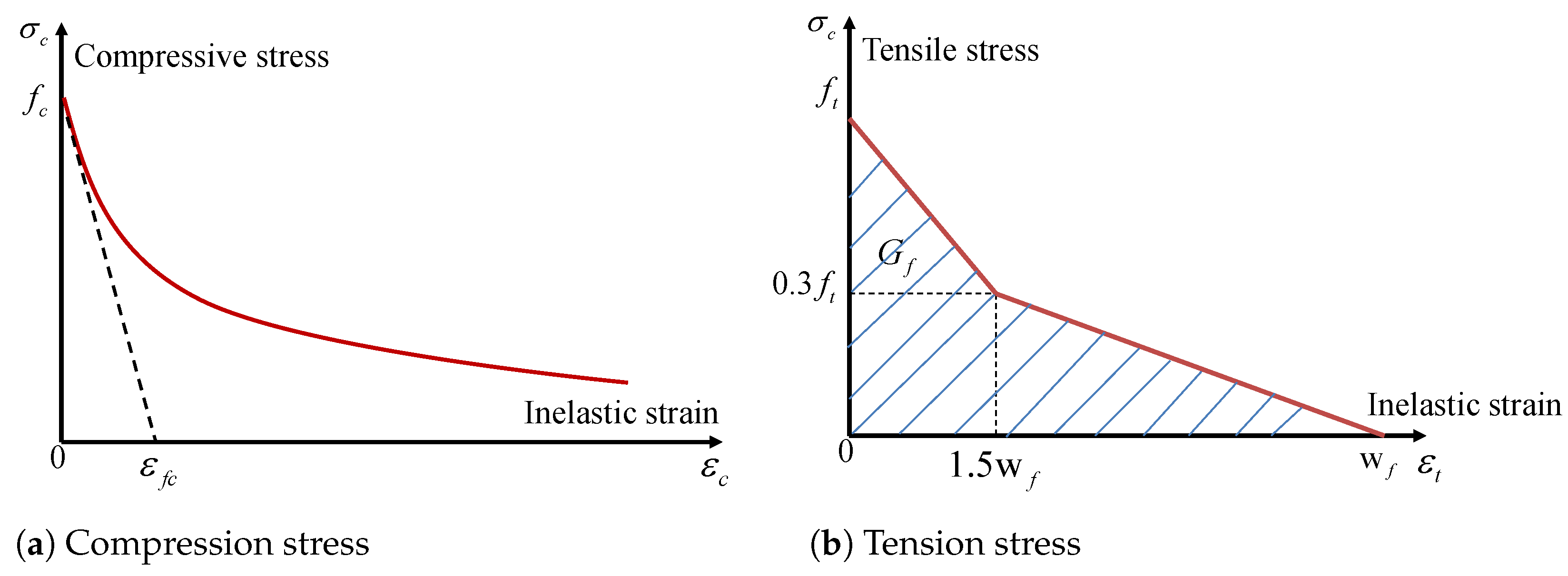
2.1. The KCC Model with Mat-Concrete Damage (MAT072R3)

The MAT072R3 model has the inbuilt ability to generate the required model input parameters in LS-DYNA based on providing the unconfined compressive strength alone that is known as the Karagozian and Case Concrete model (KCC) [39,40,41]. This model has been used in a variety of studies concentrating on quasi-static and impact loads on structures [42,43,44].

The apparent strength of concrete can dramatically rise at very high strain rates. The influence of strain rate on concrete strengths is usually expressed as a dynamic increase factor (DIF) versus strain rate, which is the ratio of dynamic to static strength. To consider the strain rate effect in the KCC model, a dynamic increase factor (DIF) was included, expressed as follows [45].

For compressive:

$$DIF=\left\{\begin{array}{cc}{\left(\dot{\epsilon }/{\dot{\epsilon }}_{sc}\right)}^{1.026{\alpha }_s},\hfill & \mathrm{for}{\epsilon }_s\le 30{\mathrm{s}}^{-1}\hfill \\ {\gamma }_s{\left(\dot{\epsilon }/{\dot{\epsilon }}_{sc}\right)}^{1/3},\hfill & \mathrm{for}{\epsilon }_s>30{\mathrm{s}}^{-1}\hfill \end{array}\right.$$

(1)

For tension:

$$DIF=\left\{\begin{array}{cc}{\left(\dot{\epsilon }/{\dot{\epsilon }}_{st}\right)}^{\delta },\hfill & \mathrm{for}{\epsilon }_s\le 1.0{\mathrm{s}}^{-1}\hfill \\ \beta {\left(\dot{\epsilon }/{\dot{\epsilon }}_{st}\right)}^{1/3},\hfill & \mathrm{for}{\epsilon }_s>1.0{\mathrm{s}}^{-1}\hfill \end{array}\right.$$

(2)

where $\dot{\epsilon }$ = strain rate in $s^{-1}$ (1/s), ${\dot{\epsilon }}_{sc}=30\times {10}^{-6}$$s^{-1}$ for a static strain rate in compression, ${\dot{\epsilon }}_{st}={10}^{-6}$$s^{-1}$ for a static strain rate in tension, $f_c$ is static compressive strength of concrete in MPa, $log\left({\gamma }_s\right)=6.156{\alpha }_s-2,{\alpha }_s=1/\left(5+0.9f_c\right),log\left(\beta \right)=6\delta -2$, and $\delta =1/\left(1+0.8f_c\right)$.

2.2. The CDP Model with Mat-CDP Damage (MAT273)

The failure behaviour of concrete under loading was depicted in the concrete damage plasticity model (CDP model) [46,47]. This model is presented for simulating the behaviour of high-strength concrete under static and dynamic loading conditions. As shown in Figure 1a, the post-peak compressive behaviour is characterized exponentially with a softening control parameter that is set to the default value $\left({\epsilon }_{fc}={10}^{-4}\right)$. The strain rate effect is studied based on the STRFLG input parameter. The strain rate effect can be considered as STRFLG = 1 and otherwise not considered (STRFLG = 0). The strain rate effects can be neglected when the hardening parameter HP is set to 0.01.

This model’s post-peak tensile behaviour can be linear, bilinear, or exponential. Because of its appropriate evaluation of experimental data [47], the bilinear damage model shown in Figure 1b was used in this study. In the figure, $G_f$ is the fracture energy defined by its underlying area of the strain softening curve; and ${\mathrm{w}}_f$ is the maximum tensile inelastic strain, which can be estimated as ${\mathrm{w}}_f=4.444G_f/f_t$ [47].

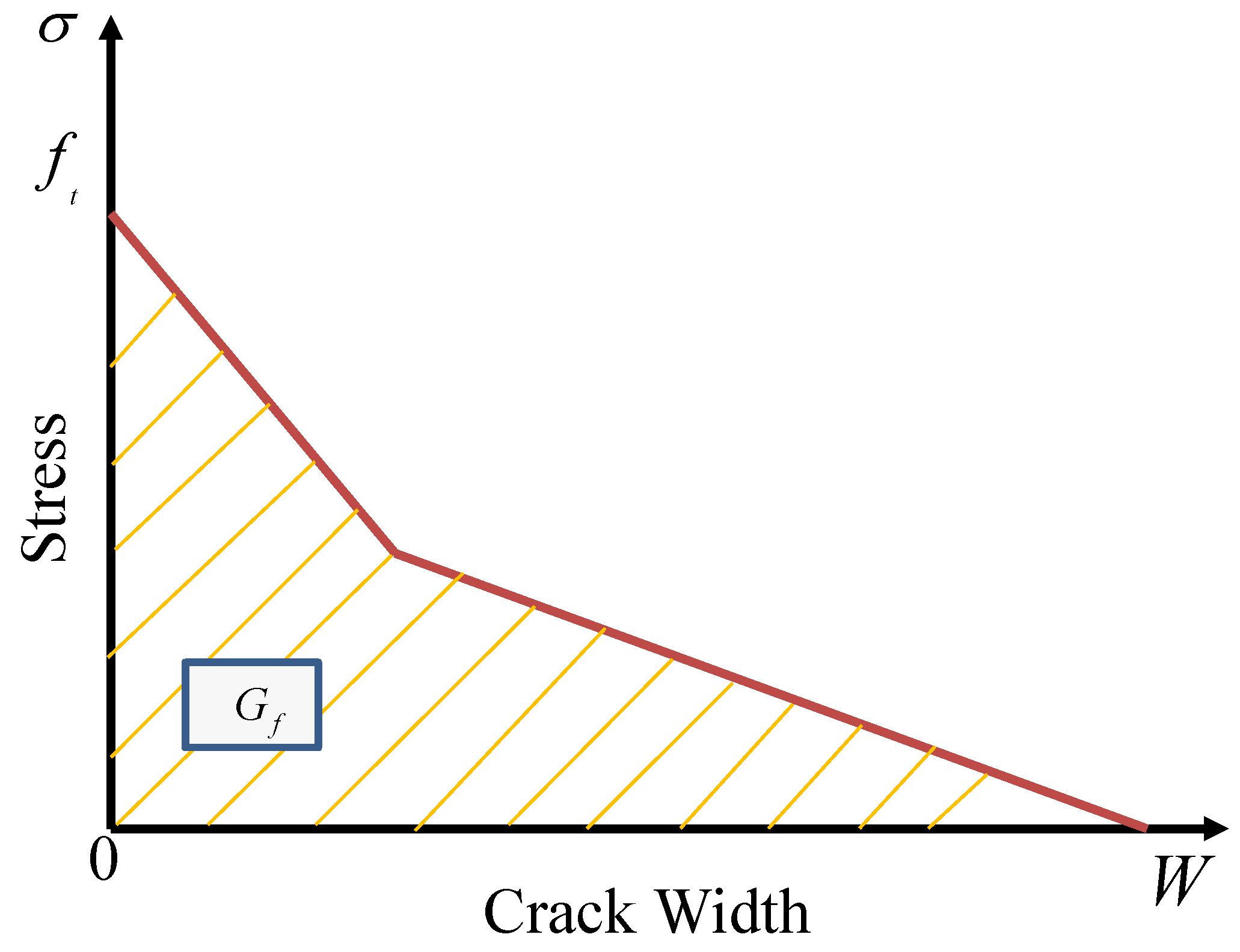
2.3. The Winfrith Model with Mat-Winfrith Damage (Mat085)

Broadhouse and Neilson [48] developed a smeared-crack model, which is the basis of the Winfrith model (“MAT WINFRITH CONCRETE” in LS-DYNA). The Winfrith model needs the user to define the unconfined compression strength ($f_c$) and tensile strength ($f_t$) as critical input parameters. The unconfined tensile strength is given by Equation (3) estimated from uniaxial compressive strength.

One of the most important features of the Winfrith concrete model is the ability to generate a binary output database for crack specifics, such as position and dimension. The crack width (W) can be defined by investigating the area under the uniaxial tensile stress versus crack width curve equal to the fracture energy ($G_f$) using Equations (4) and (5) as shown Figure 2. The RATE Winfrith input parameter controls whether the strain rate effect is studied (RATE = 0) or not (RATE = 1, 2). The difference between RATE = 1 and 2 is that RATE = 2 examines improved crack algorithms.

$$f_t=1.4{\left(\frac{f_c}{10}\right)}^{2/3}$$

(3)

$$G_f=73f_c^{0.18}$$

(4)

$$W=\frac{2G_f}{f_{\mathrm{t}}}$$

(5)

3. Analytical Methodology Validation

3.1. Experimental Investigation

Pakiding et al. [49] and Beyer et al. [50] conducted experimental tests on the Post-Tensioned and 3D RC walls, respectively. The main purpose of the experiments was to consider the capability of sustaining large deformations before failure for PT reinforced concrete wall as well as to investigate the bending behaviour in different directions for a 3D wall subjected to a bi-directional loading. The post-tensioned and 3D RC walls are frequently used in high buildings as lateral strength providing members which support load-bearing capability in the structure. These experimental results provide a foundation for future study to examine and forecast the behaviour of walls during earthquakes.

The PT 2D wall is 1830 mm (length) × 6730 mm (height) × 250 mm (thickness). The foundation block for the wall is 7620 mm × 1520 mm × 610 mm. The wall was made up of eight 22-mm diameter longitudinal bars and two 9.5-mm diameter longitudinal bars. The 3D wall is 1600 mm (length) × 3490 mm (height) × 160 mm (thickness). The longitudinal reinforcement was maintained throughout the wall’s height with continuous bars running from the foundation to the collar (no lap splices). The vertical reinforcement had a total area of approximately $A_s=3281{\mathrm{mm}}^2$.

The material properties for the concrete with the compressive strength were 43 MPa for the PT wall and 45 MPa for the 3D wall. The steel reinforced with a nominal yield strength of 414 MPa was based on ASTM A615 and ASTM A706 standards for PT walls. Moreover, the 3D wall used reinforcing bars based on the requirements for “Class C” grade steel according to Eurocode 8 with a yield strength of 488 MPa for diameter of 12 mm and 518 MPa for a diameter of 6 mm.

3.2. Constitutive Material Models

The material characteristics of the concrete constitutive model are calibrated consistently. The uniaxial compressive strength, $f_c$, is estimated using material testing in conjunction with structural component tests. For all analytical models, the Poisson’s ratio is fixed to 0.2. The material specifications for the concrete models are listed in

Table 1. Concrete material model parameters.

Specimen	${\mathit{E}}_{\mathit{s}}$	${\mathit{f}}_{\mathit{c}}$	$\mathit{\rho }$	$\mathit{\nu }$
	(MPa)	(MPa)	$\left(\mathbf{g}/{\mathbf{mm}}^3\right)$
Pakiding et al. [49]	200,000	43.4	0.0023	0.2
PT 2D wall
Beyer et al. [50]	200,000	45.0	0.0023	0.2
3D wall

.

The steel material in this study can be modelled in LS-DYNA using MAT#03 (*MAT_ PLASTIC_KINEMATIC), which is suitable for both isotropic and kinematic hardening plasticity simulations [51]. In

Table 2. Steel material parameters.

Specimen	Bar	${\mathit{E}}_{\mathit{s}}$	$\mathit{\rho }$	$\mathit{\nu }$	${\mathit{f}}_{\mathit{y}}$	${\mathit{f}}_{\mathit{u}}$
	Type	(MPa)	$\left(\mathbf{g}/{\mathbf{mm}}^3\right)$		(MPa)	(MPa)
Pakiding et al. [49]	#1	200,000	0.00783	0.3	519	744
PT 2D wall	#2	200,000	0.00783	0.3	473	742
	#3	200,000	0.00783	0.3	473	742
	#4	200,000	0.00783	0.3	441	683
	#5	200,000	0.00783	0.3	1675	2038
Beyer et al. [50]	#6	200,000	0.00783	0.3	519	744
3D wall	#7	200,000	0.00783	0.3	518	681

The following should be noted: f_c is the concrete compressive strength, $\rho$ is the mass density, $\nu$ is Poisson’s ratio, E_s is Young’s modulus, f_y and f_u are the rebar yield stress and ultimate strength, respectively.

, the material parameters for reinforcing steel are listed. For all analyses, the Poisson ratio, $\nu$, is set at 0.3, which is also required in the continuum-based beam elements.

The loading section on top and the wall footing material were considered to be elastic for the purpose of simplicity and to concentrate on the behaviour of the walls *MAT_ELASTIC was used to model the base and top parts in LS-DYNA.

3.3. Contact and Boundary Conditions

The reinforcements were embedded in the concrete walls using the *CONSTRAINED_ LARGRANGE_ IN_ SOLID option [52]. This option models perfect bonding conditions between the reinforcements and the surrounding concrete. The Dynamic Implicit analysis approach was employed in this study as reported in [51]. The global response is modelled as a dynamic problem, and the equations of motion in time are integrated using the central difference method. At each stage of the investigation, the equations of motion are solved using the mesh’s changed geometry.

4. Numerical Analysis and Comparison with Experimental Results

4.1. Analysis of PT 2D Wall under Pushover Analysis

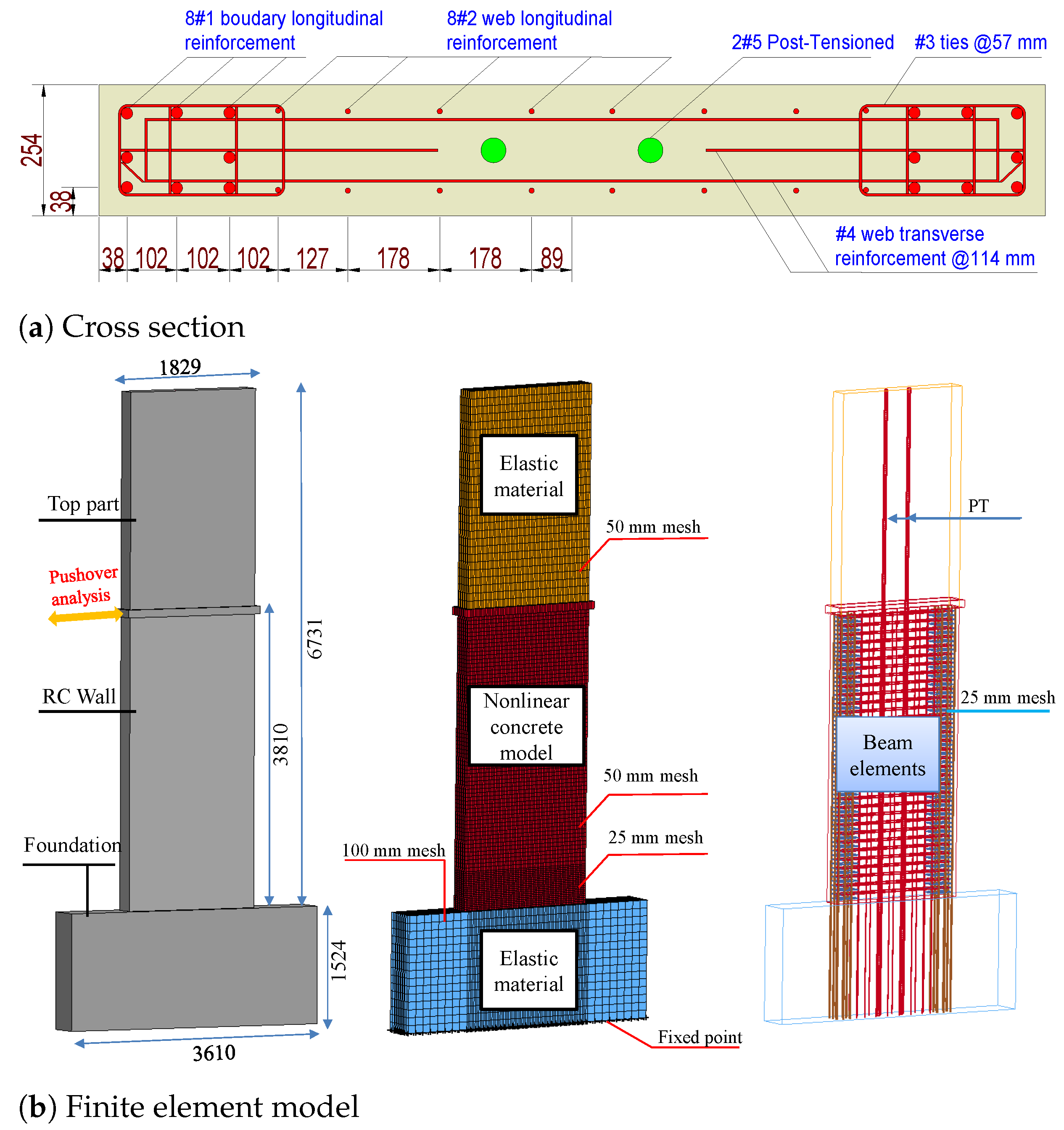
4.1.1. Geometric and Finite Element (FE) Model

This section evaluates the validity of several concrete material models. The authors of [53,54,55,56] have proved the reliability of material models in forecasting the response of PT reinforced concrete walls. Experimental data is compared to research findings. Pakiding et al. [49] evaluated PT reinforced concrete wall specimens and completed the analysis. The wall’s configuration details are shown in Figure 3. Two prestressing tendon bundles, each with five strands, were employed to give a prestressing force of 1561 kN with a diameter of 15.2 mm. In the web and boundary portions of the section, the wall contained sixteen #1 bars with a diameter of 22 mm and vertical #3 bars with a diameter of 10 mm, as well as extra horizontal reinforcement #4 with a diameter of 10 mm. Pushover loading was applied to the wall specimen at a height of 3810 mm from the foundation block until damage occurred.

Figure 3b shows the FE models of the PT 2D wall. An eight-node solid element was used to model the concrete wall, top section, and foundation. Figure 3b shows the PT 2D wall reinforcements, which were calculated using a beam element with a cross-section integration (Hughes–Liu beam) [12]. In the face of severe deformations, this formulation method is well known for being efficient, accurate, and effective. Based on the experimental results, the modeling strategy was established to reduce the computational time. The wall model is divided into two regions such as elastic for foundation and the top part as well as inelastic for the RC wall part. This is because the significant damage on the upper part and the foundation was not observed during the test.

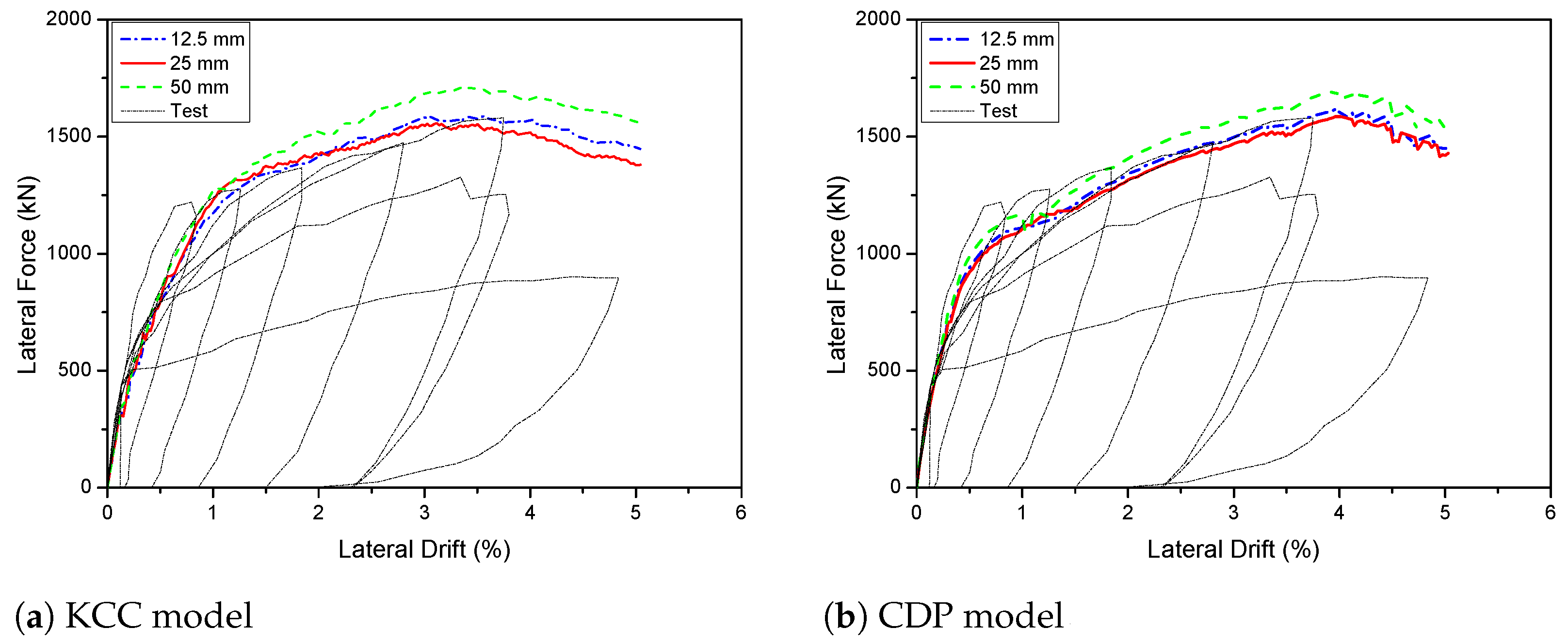
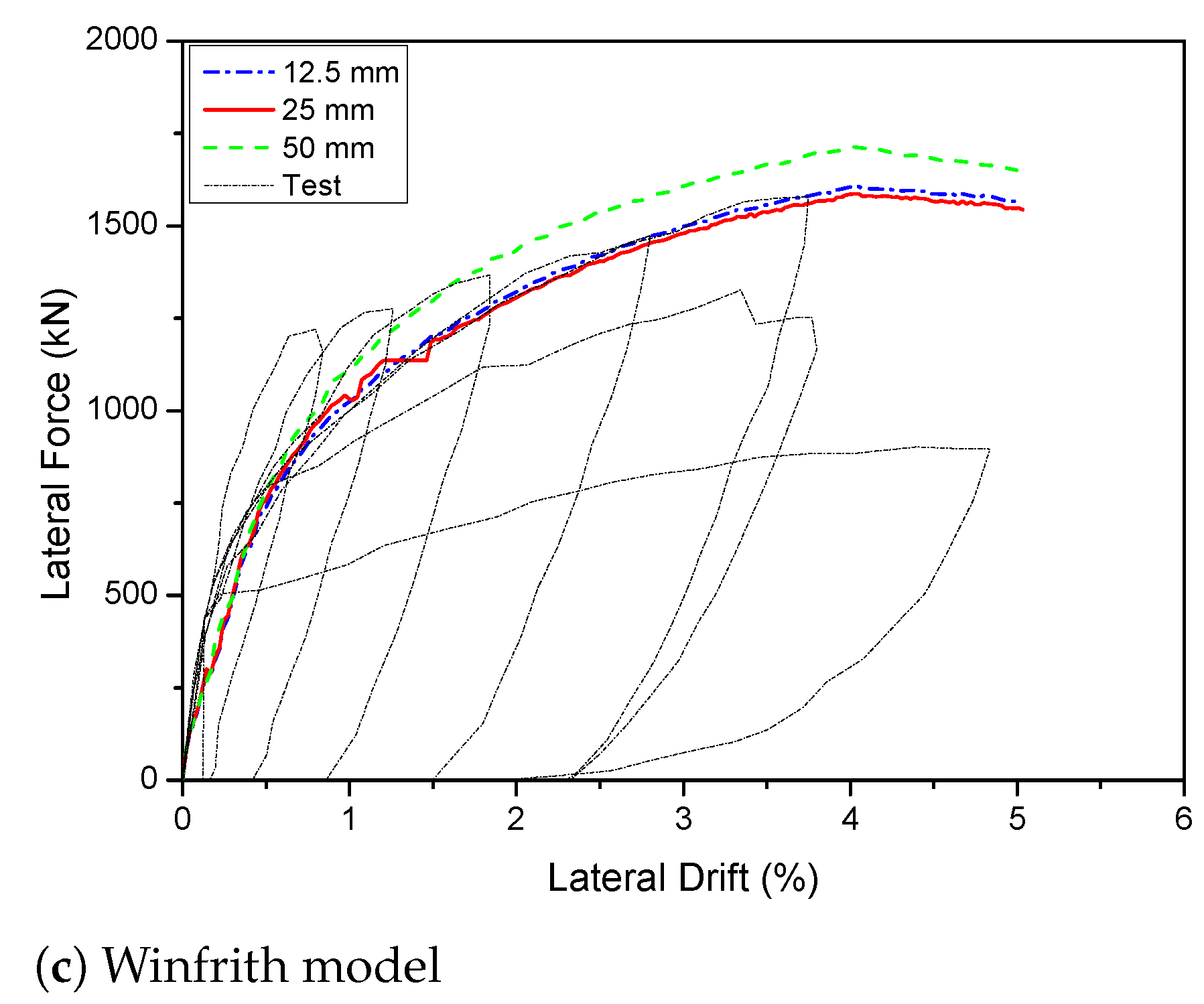
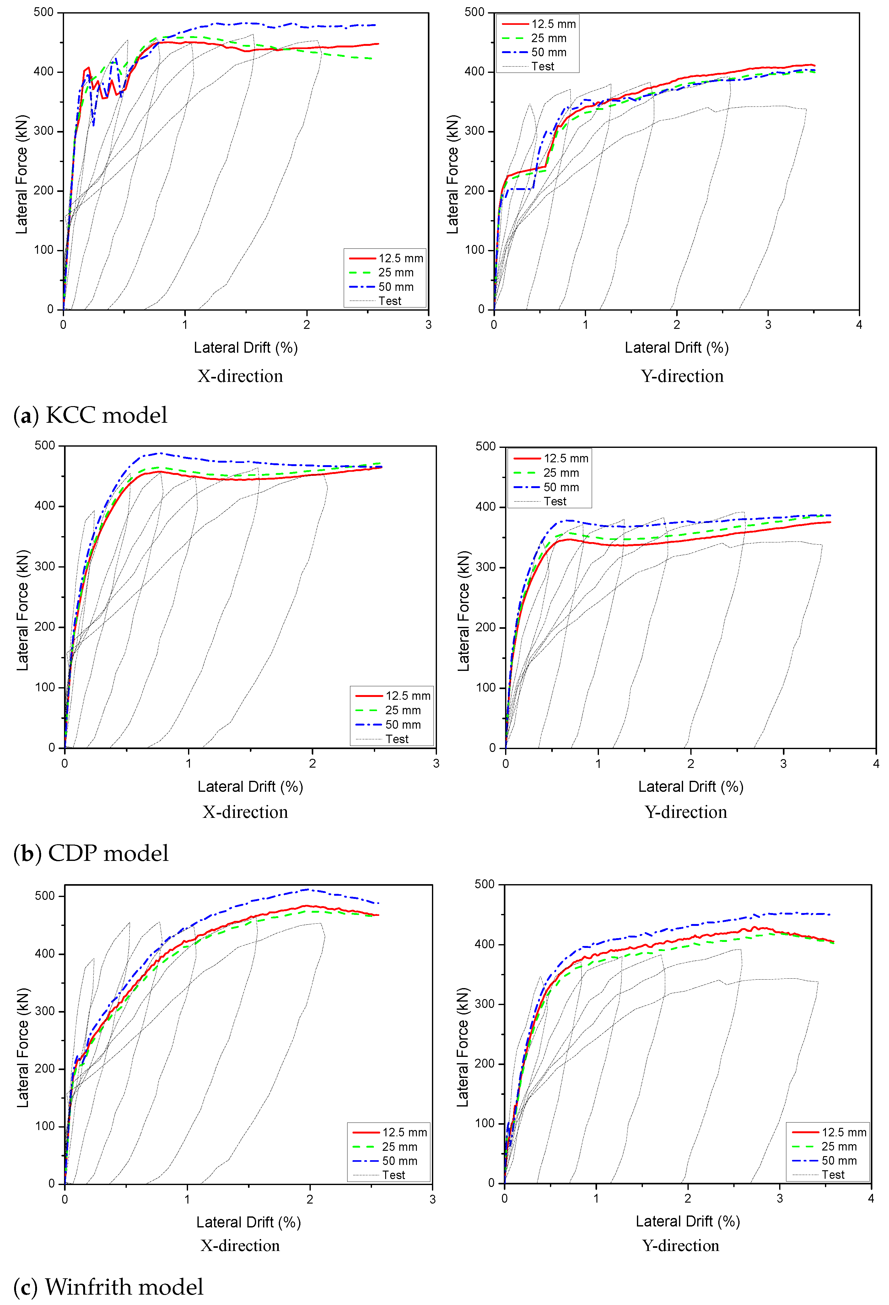
4.1.2. Effect Type of Mesh Size Element

The mesh size is proportional to the precision and number of meshes required to mesh the element in Finite Element Analysis. Mesh size has an influence not only on the accuracy of the results, but also on the analytical time of the model. As a result, investigating the influence of mesh size is crucial. The model can calculate faster and offer more accurate results with the correct mesh size.

Figure 4 depicts the findings of a mesh size influence study including three distinct mesh sizes: 12.5 mm, 25 mm, and 50 mm. The force–displacement relationships do not improve considerably as the mesh sizes are 12.5 mm and 25 mm. The concrete wall was divided into two sections meshed with a 25 mm and 50 mm size, and the beams were meshed with a 25 mm size to reduce computing time. As shown in Figure 3b, the foundation and upper part elements had a larger mesh size (e.g., 100 mm) than the primary structural elements (i.e., wall, beam).

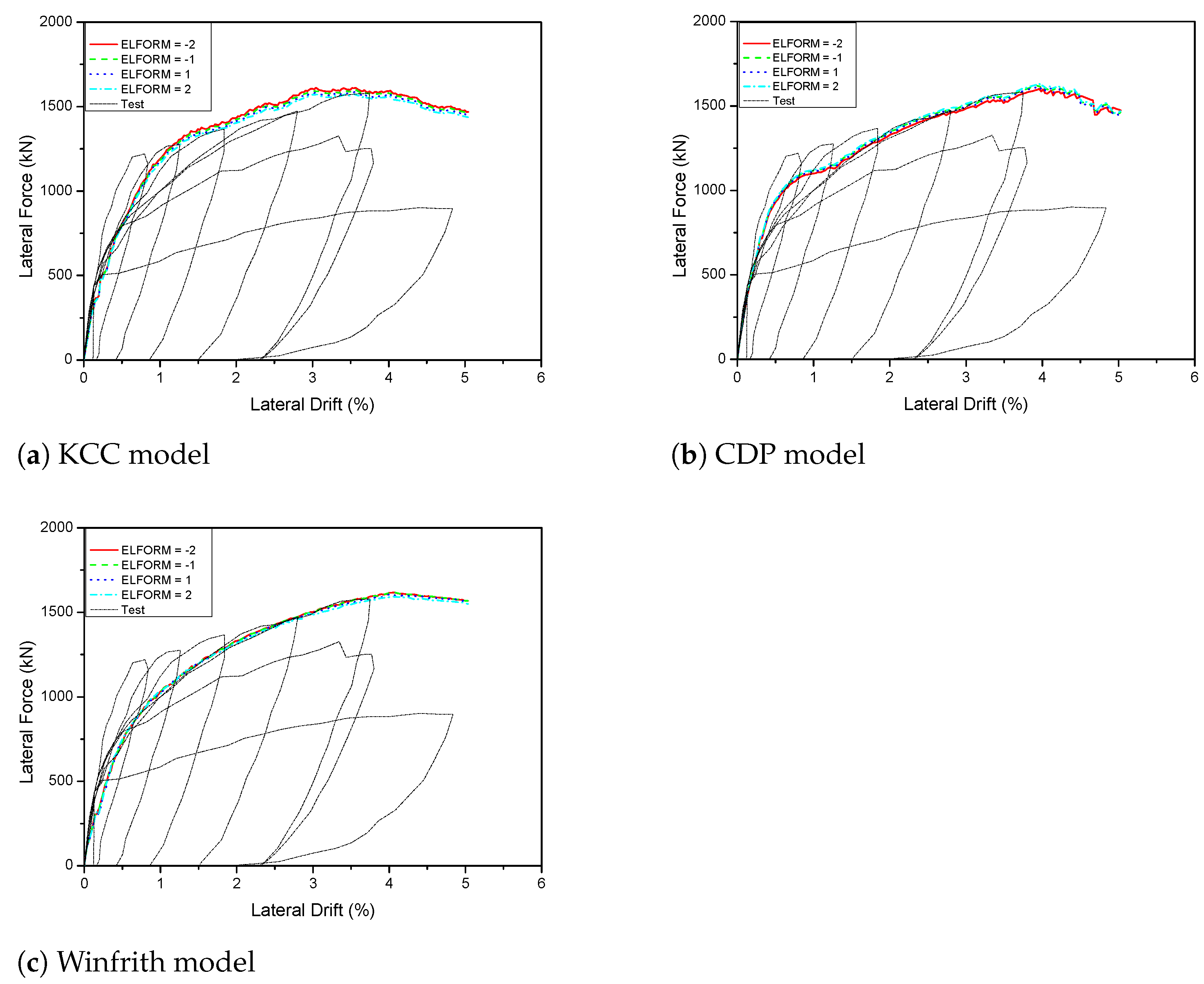
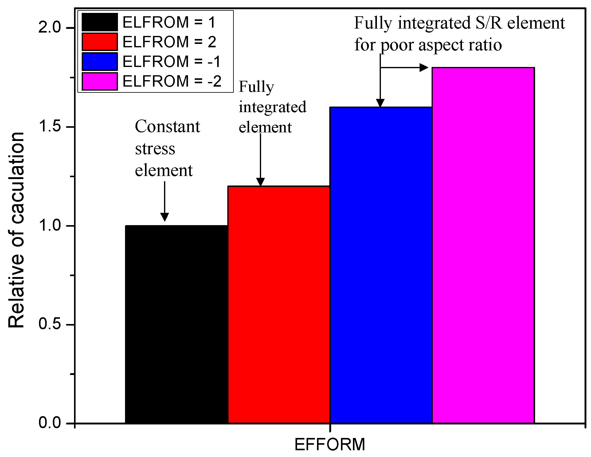
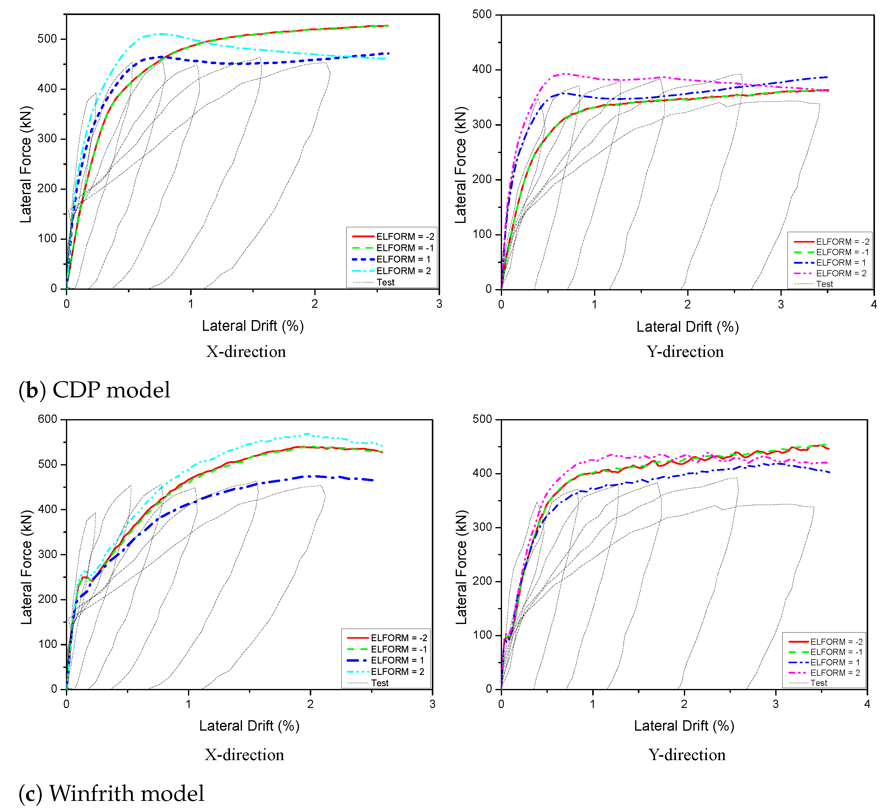
4.1.3. Effect Type of Concrete Element

The concrete behaviour was simulated using an eight-node reduced integrated solid element. In LS-DYNA, there are four different sorts of solid elements: The fully integrated S/R solid element for poor aspect ratio with accurate and efficient formulations, respectively $(\mathrm{ELFORM}=-2\mathrm{and}-1)$, fully integrated S/R solid element (ELFORM = 2), and constant stress solid element (ELFORM = 1) are commonly used solid element types in LS-DYNA.

The investigations for these four element types are compared with the PT 2D wall experimental data in Figure 5. Almost all of the models correctly predicted specimen resistance, according to the comparison. However, as shown in Figure 6, the constant stress solid element (ELFORM = 1) provided the quickest relative calculation time of the four models. It took at least 1.2 times as long to simulate with a fully integrated S/R solid element as it did with a constant stress solid element. In terms of calculation, this element is both precise and efficient. As a result, the constant stress solid element was chosen for this study.

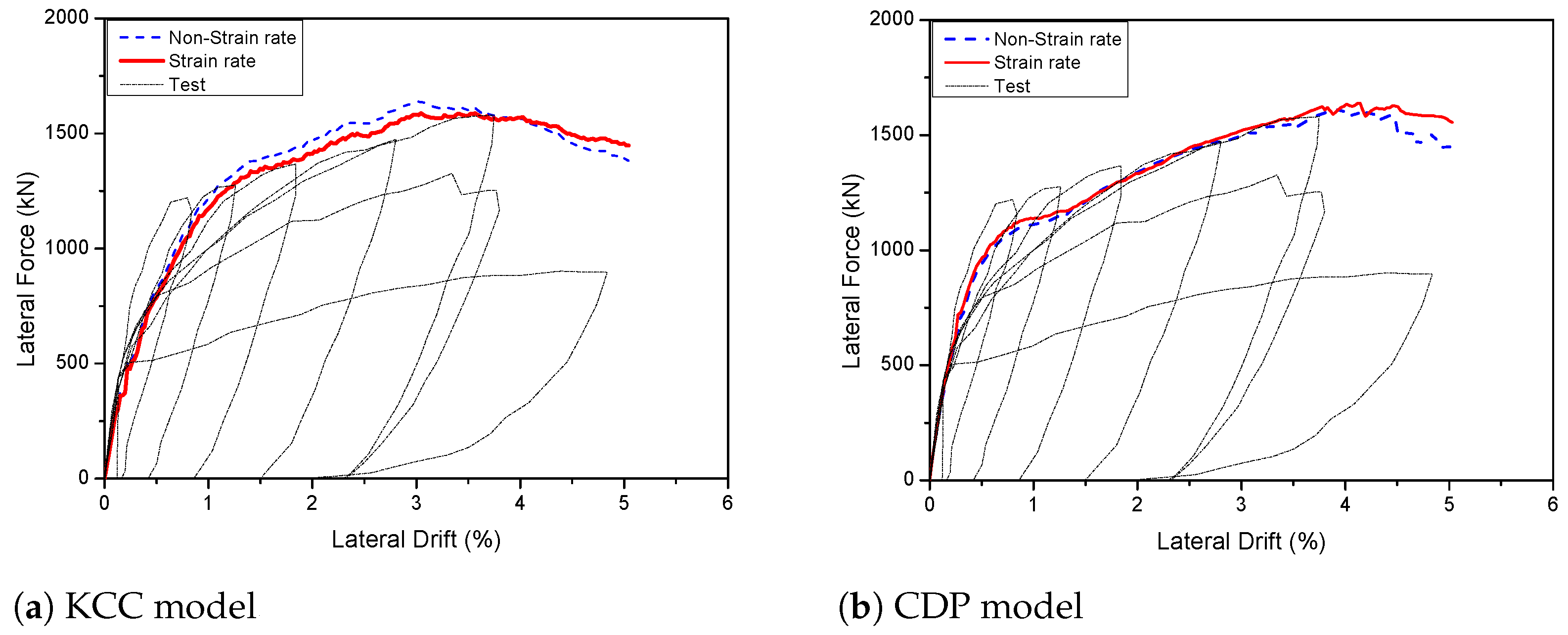
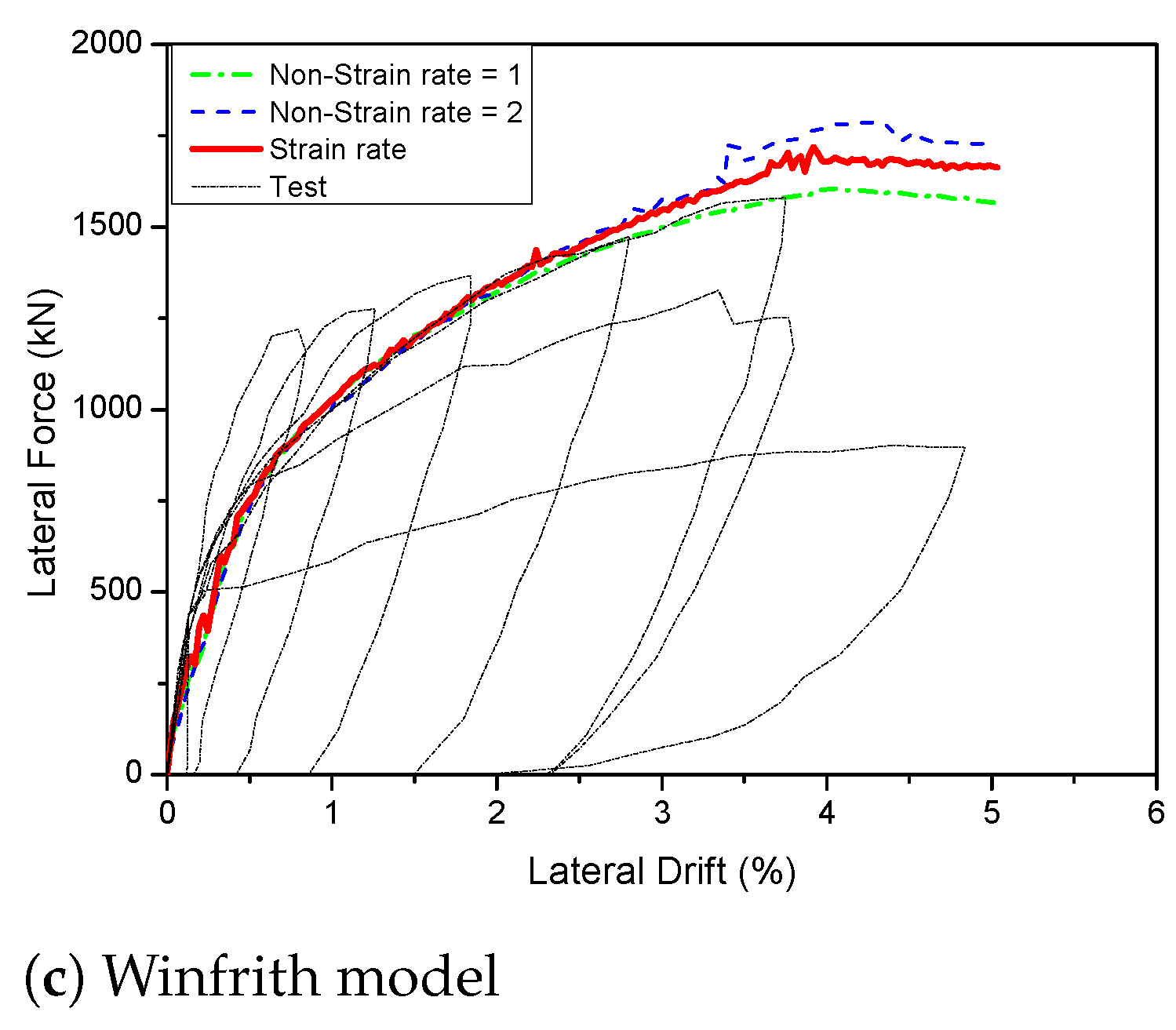
4.1.4. Effect of Strain Rate

Many different parameters influence the model’s response, with the strain rate being one of the most directly influencing factors for concrete behavior. The rate effect is used to describe a material’s reliance on loading or strain rates. In LS-DYNA, a built-in parameter that is based on several concrete models represents the strain rate influence on concrete strength. By activating the strain rate formulation, increased strain rate increases the concrete material’s strength. Using viscoplastic parameters, the rate effect is applied to the plasticity surface, damage surface, and fracture energy. To guarantee that uniaxial tensile and compressive strength values are compatible, the viscoplastic parameters are applied. It is critical to employ a computational model that reliably replicates the transition between diffuse damage, crack initiation, and crack propagation in order to accurately simulate the dynamic and viscoelastic response of concrete structures with the strain rate effect. The model can still bear shear, compressive, and tensile loads after the first crack has occurred. As a result, the concrete behaviour will be more realistically replicated under tensile stress. The DIF ratio is used to explore the strain rate effects of the KCC models, and the CDP models are considered at various rates such as STRFLG = 0, STRFLG = 1. On the other hand, the Winfrith models were focus on various rate effects, such as RATE = 0, RATE = 1, and RATE = 2.

The force–displacement findings of PT 2D walls with strain rate effects are as shown in Figure 7. The strain rate effects have no effect on the force–displacement relationships of the KCC and CDP models, whereas the Winfrith models were affected by strain rate and were best used with RATE = 1. The key parameters of the hysteresis diagrams are as shown in

Table 3. The maximum lateral force of the hysteresis diagram of PT 2D walls (kN).

Model	Mesh Size			ELFORM				Strain Rate
	12.5 mm	25 mm	50 mm	$-\mathbf{2}$	$-\mathbf{1}$	1	2	a	b	c
KCC	1558 (0.2%)	1588 (1.7%)	1711 (9.6%)	1612 (3.3%)	1600 (2.5%)	1588 (1.7%)	1578 (1.1%)	1650 (5.7%)	1590 (1.9%)	-
CDP	1586 (1.6%)	1617 (3.6%)	1698 (8.8%)	1602 (2.6%)	1624 (4.1%)	1617 (3.6%)	1632 (4.5%)	1640 (5.1%)	1620 (3.8%)	-
Winfrith	1589 (1.8%)	1607 (2.9%)	1714 (9.8%)	1617 (3.5%)	1617 (3.5%)	1608 (3.0%)	1595 (2.2%)	1720 (10.2%)	1610 (3.1%)	1790 (14.7%)
Test	1561 (kN)			1561 (kN)				1561 (kN)

The following should be noted: a is strain rate effect, b is not strain rate effect, c is not strain rate effect but includes improved crack algorithm (for Winfrith model).

.

4.1.5. Failure Behaviour

The maximum principal strain fringe, which can be calculated using LS-DYNA, was utilized to investigate the concrete damage mechanism and pattern. The maximum principal strain contours of models can be used to identify the regions of maximum flexural stresses in beams. Because different material models have varied strain ranges, the contour ranges are also provided for each situation. Figure 8 illustrates structural damage reproduced from the finite element model for the PT 2D wall. Based on the color palette in the maximum principal strain fringe to calculate the damage area in the wall, this figure depicts concrete and reinforcement damage. As shown in Figure 8a, the KCC model appears to be unable to detect localized concrete failure or the maximum tensile zone in rebars because the color range seen in this illustration is located in the center of the primary color palette. The CDP model can also see the failure occurring at the wall’s corner and the regions of maximum flexural stresses in beams based on the color palette in the maximum principal strain fringe, as shown in Figure 8b. On the other hand, because the color area for concrete and rebars is identified at the peak of the color palette in the maximum primary strain fringe, the failure site and maximum tensile regions in rebars could be reasonably approximated for the Winfrith model. As seen in Figure 8c, the damage occurs around the base due to the presentation of contours. As a results, the CDP and Winfrith models can reproduce the damage location and pattern as compared to the experimental results observed from Pakiding et al [49].

4.2. Analysis of 3D Wall under Pushover Analysis

4.2.1. Hysteresis and Backbone Curves

Because their shape provides strength and stiffness in any horizontal direction while also being well adapted to enable elevator shafts or staircases, 3D reinforced concrete walls are often used as lateral strength supplying components in reinforced concrete (RC) buildings. The 3D reinforced concrete wall specimen, also known as the TUA test by Beyer et al. [50], is the next validation analysis. As illustrated in Figure 9a, the wall’s height and thickness were 2650 mm and 150 mm, respectively. This model will be used to describe bidirectional loads in the X and Y directions. The configuration details of the wall are depicted in Figure 9b. In the boundary areas of the wall, there were twenty-two #6 bars with a diameter of 12 mm, and in the web regions of the section, there were twenty-eight #7 bars with a diameter of 6 mm. In addition, ties with a diameter of 6 mm and a spacing of 125 mm were used at the wall boundaries and web portions of the wall, with a diameter of 6 mm and a spacing of 50 mm. The wall specimen was tested using a prescribed monotonic bidirectional displacement history that was applied at 3350 mm and 2950 mm for loading X and Y directions, respectively, until damage occurred. Figure 9c shows the FE model of a wall specimen. The concrete wall, top portion, and base were all modelled using an eight-node solid element. A beam element with a cross-section integration (Hughes-Liu beam) was also used to calculate the RC wall reinforcements.

Under pushover loading, the 3D wall was tested on three concrete models. In Figure 10, Figure 11 and Figure 12, the analytical results of the 3D wall utilizing various concrete models such as KCC, CDP, and Winfrith are compared to the corresponding experimental data. To validate the mesh size effects, the experimental findings were compared to the hysteresis and backbone curves derived from the FEA with three sizes: 12.5 mm, 25 mm, and 50 mm, as shown in Figure 10. The force–displacement relationships do not change significantly since the mesh size for the displacement–force curve in the X direction in three models is 12.5 mm and 25 mm, whereas the mesh size for the Y direction results is 12.5 mm, 25 mm, and 50 mm. The concrete wall was divided into two parts meshed with a 25 mm and 50 mm size, and the beams were meshed with a 25 mm size to reduce computing time. As shown in Figure 9c, the foundation and upper part elements had a larger mesh size (e.g., 100 mm) than the primary structural elements (i.e., wall, beam). As indicated in Figure 11 and Figure 12, the concrete element and strain rate had a profound influence on the displacement–force curve results. In LS-DYNA, there are four sorts of solid elements that are widely used: The solid element types ELFORM = 2, −1, 1 and 2 are often employed. In three models, the concrete element (ELFORM = 1) was a reasonable forecast for the displacement–force curve in both the X and Y directions, as illustrated in Figure 11. The CDP and Winfrith models performed well because they did not account for the strain rate effect in both the X and Y directions, and RATE = 1 was appropriate for the Winfrith model. The KCC model, on the other hand, provided an acceptable forecast for both the X and Y directions, as shown in Figure 12.

Table 4. The maximum lateral force of the hysteresis diagram of 3D walls for the X Direction (Unit: kN).

Model	Mesh Size			ELFORM				Strain Rate
	12.5 mm	25 mm	50 mm	$-\mathbf{2}$	$-\mathbf{1}$	1	2	a	b	c
KCC	459.9 (0.2%)	450.9 (1.8%)	482.6 (5.1%)	495.7 (8.0%)	500.9 (9.1%)	450.9 (1.8%)	508.0 (10.7%)	450.9 (1.8%)	468.6 (2.1%)	-
CDP	464.7 (1.2%)	472.0 (2.8%)	487.9 (6.3%)	527.3 (14.8%)	526.9 (14.8%)	472.0 (2.8%)	511.2 (11.4%)	512.1 (11.6%)	464.7 (1.3%)	-
Winfrith	484.1 (5.5%)	474.6 (3.4%)	512.6 (11.7%)	539.9 (17.6%)	542.1 (18.1%)	474.6 (3.4%)	569.4 (24.1%)	420.0 (8.5%)	474.6 (3.4%)	512.1 (11.6%)
Test	459.0 kN			459.0 kN				459.0 kN

The following should be noted: a is strain rate effect, b is not strain rate effect (RATE = 1), c is not strain rate effect (RATE = 2) but includes improved crack algorithm.

and

Table 5. The maximum lateral force of the hysteresis diagram of 3D walls for Y Direction (Unit: kN).

Model	Mesh Size			ELFORM				Strain Rate
	12.5 mm	25 mm	50 mm	$-\mathbf{2}$	$-\mathbf{1}$	1	2	a	b	c
KCC	401.4 (2.0%)	412.7 (4.9%)	404.3 (2.7%)	452.2 (14.9%)	456.7 (16.1%)	412.7 (4.9%)	450.2 (14.4%)	412.7 (4.9%)	404.3 (2.7%)	-
CDP	375.5 (4.6%)	386.8 (1.7%)	378.9 (3.7%)	363.6 (7.6%)	364.2 (7.4%)	386.8 (1.7%)	393.2 (0.1%)	376.6 (4.3%)	386.8 (1.7%)	-
Winfrith	429.5 (9.1%)	418.8 (6.4%)	454.3 (15.5%)	452.3 (14.9%)	454.6 (15.5%)	418.8 (6.4%)	439.4 (11.7%)	362.6 (7.9%)	418.8 (6.4%)	450.9 (14.6%)
Test	393.5 kN			393.5 kN				393.5 kN

The following should be noted: a is strain rate effect, b is not strain rate effect (RATE = 1), c is not strain rate effect (RATE = 2) but includes improved crack algorithm.

show the findings of the maximum displacement–force hysteresis diagrams.

4.2.2. Failure Behaviour

The maximum principal strain fringe will be used to examine the damage mechanism and pattern of this model. The color palette is to be used in the maximum primary strain fringe to calculate the damage zone in the wall, including the damaged concrete and rebars, similar to the explored standard for 2D wall damage. Figure 13 illustrates structural damage reproduced from the finite element model for the 3D wall. The KCC model can predict maximum tensile regions in beams and recognize localized failure, but it is not totally correct for concrete failure since the color range visible for concrete only extends to the top of the main color palette, as shown in Figure 13a. The CDP and Winfrith models, on the other hand, can reliably detect the location of concrete failure as well as the maximum tensile regions in rebars by detecting the color range for concrete and rebars at the peak of the color palette in the maximum principal strain fringe, as shown in Figure 13b and Figure 13c, respectively.

5. Effect of PT Bars for Reinforced Concrete Walls

The validated FE model was used to perform further parametric study on the structural performance of PT 2D and 3D walls. The investigation focused primarily on the influence of the PT bars part under pushover analysis. The designated parameters considered in this task were (1) the PT quantities, (2) the PT diameters, and (3) the PT yield strength.

5.1. Effect of PT Bars for PT 2D Wall

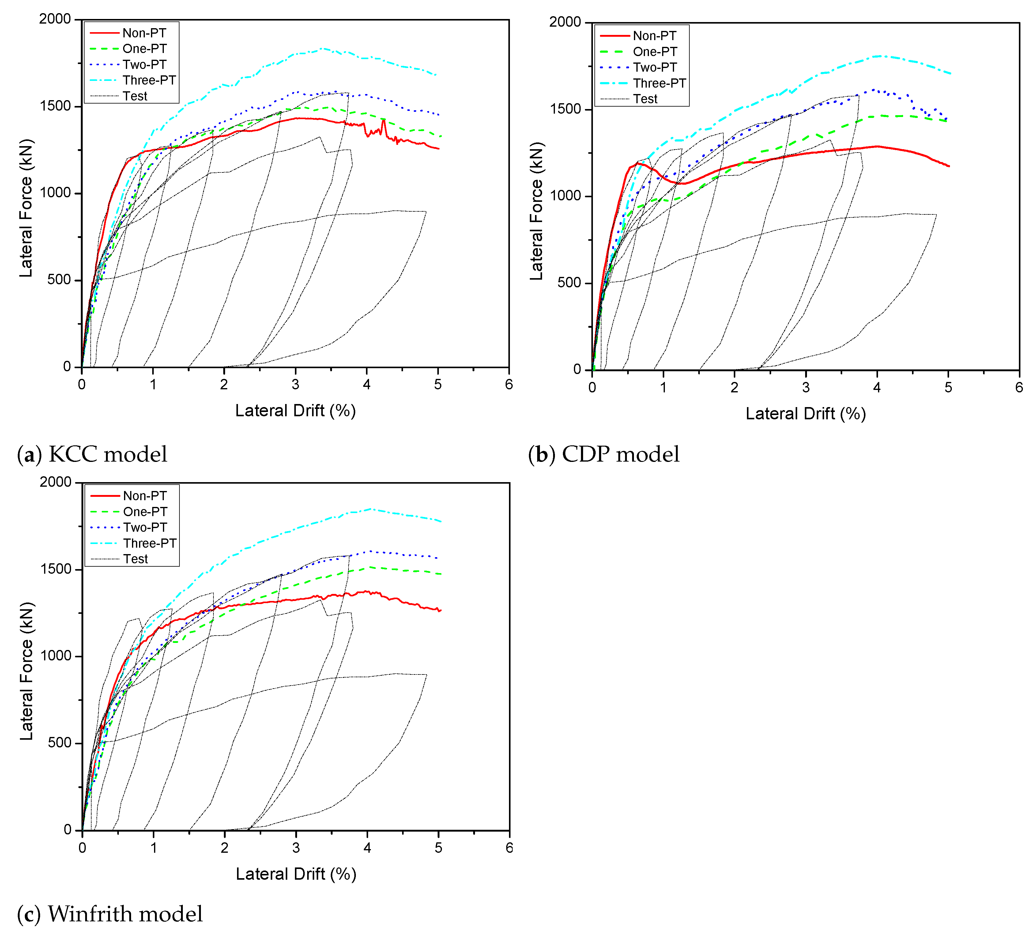
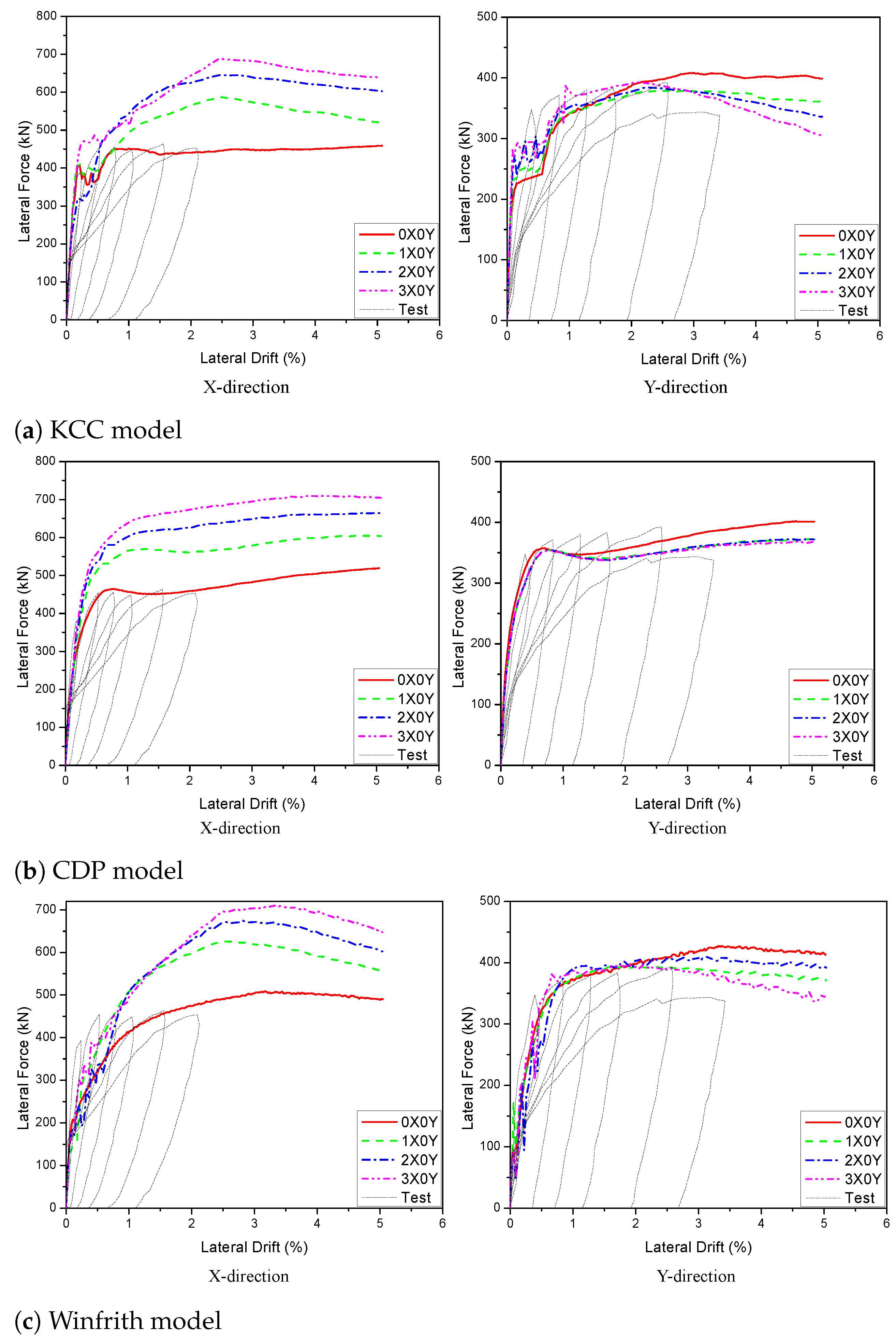
5.1.1. Effect of PT Quantities

As shown in Figure 14, the PT quantities were explored in four scenarios: Non-PT, one PT, two PT, and three PT. Figure 15 depicts the influence of the PT quantities on the load–displacement curve. In general, raising the PT quantities improved the specimen’s maximum lateral load in all samples. The curve had a trend significantly increasing in the first period of lateral drift (0–1%) and obtaining the maximum lateral force in the period of lateral drift of 3–4%. Because the CDP concrete model was the sensitive model for the stiffness, the entire structural stiffness had a significant change as using non-PT. As a result, the maximum strength was obtained in the first period of lateral drift (0–1%). According to these plots, when the lateral strength was increased from two to three PT, the KCC model improved from 1588.34 kN to 1834.1 kN (15.5%), the CDP model improved from 1616.8 kN to 1809.8 kN (11.9%), and the Winfrith model improved from 1606.8 kN to 1850.7 kN (15.2%). When the lateral strength of the KCC, CDP, and Winfrith models was reduced from two to one PT, the lateral strength was reduced by 5.4%, 9.3%, and 5.7%, respectively, as shown in Figure 16. When the lateral strength of the KCC, CDP, and Winfrith models was reduced from two to no PT, the lateral strength was reduced by 9.7%, 20.3%, and 14.3%, respectively. The lateral strength changed depending on whether the PT quantities were increased or decreased, but it was discovered that using PT quantities from two to three PT resulted in larger force changing than using PT quantities less than two PT.

Table 6. The different maximum lateral force of PT quantities of PT 2D walls.

PT Quantities	KCC Model		CDP Model		Winfrith Model
	Values (kN)	Errors (%)	Values (kN)	Errors (%)	Values (kN)	Errors (%)
Three PT	1834.1	15.5	1809.8	11.9	1850.7	15.2
Two PT	1588.3	-	1616.8	-	1606.8	-
One PT	1502.1	−5.4	1466.5	−9.3	1514.8	−5.7
Non-PT	1433.9	−9.7	1288.8	−20.3	1376.8	−14.3

shows the detailed parameters.

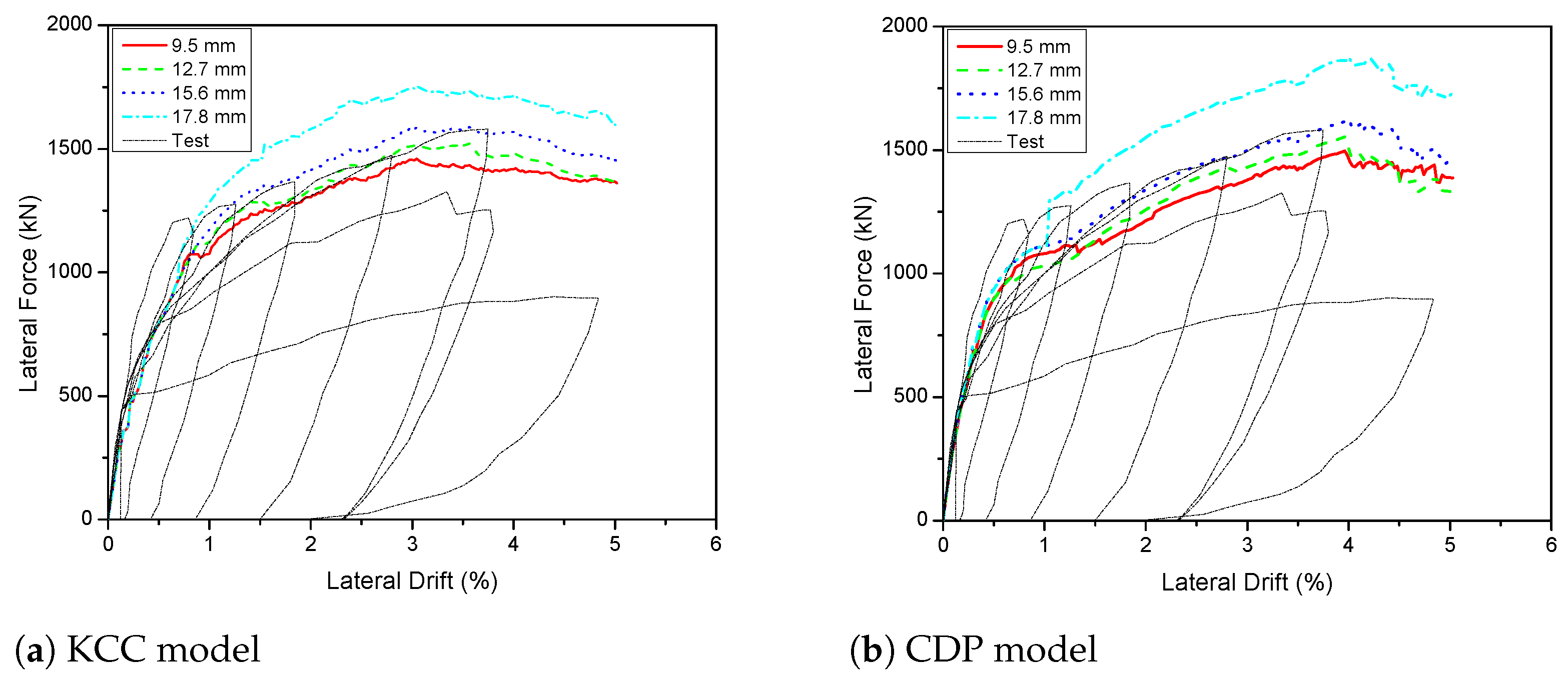
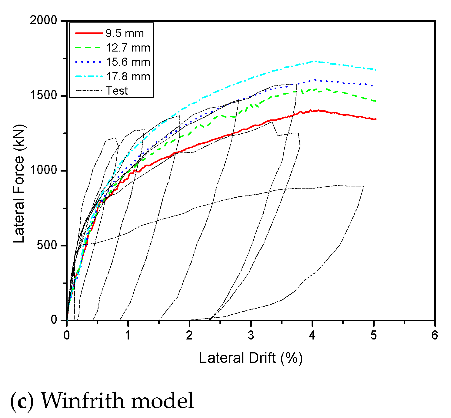
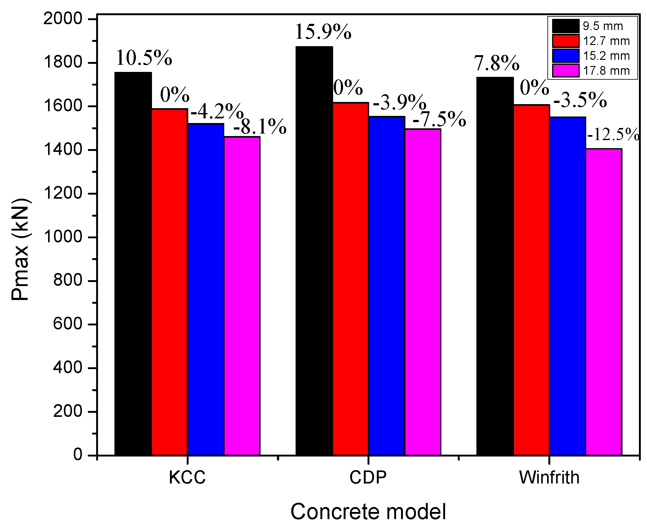
5.1.2. Effect of PT Diameter

The responses of the PT 2D wall behavior were tested using four different PT diameter scenarios: 9.5 mm, 12.7 mm, 15.6 mm, and 17.8 mm. Figure 17 shows the influence of the post-tensioned diameter on the load–displacement curve. In general, changing the PT diameters improved the maximum lateral load of the specimen in this figure. According to these figures, when the diameter was extended from 15.2 mm to 17.8 mm, the lateral strength of the KCC model grew from 1588.3 kN to 1754.8 kN (10.5%), the CDP model increased from 1616.8 kN to 1873.4 kN (15.9%), and the Winfrith model increased from 1606.8 kN to 1732.6 kN (7.8%). The lateral strength of the KCC, CDP, and Winfrith models reduced 4.2%, 3.9%, and 3.5%, respectively, as the diameter was changed from 15.2 mm to 12.7 mm. The lateral strength of the KCC, CDP, and Winfrith models was reduced by 8.1%, 7.5%, and 12.5%, respectively, as the diameter was reduced from 15.2 mm to 9.5 mm. According to the varied changes in lateral strength, the 15.2 mm and 17.8 mm diameters are the best choices for increasing lateral strength carrying capacity for the PT 2D wall, as shown in Figure 18. The details of the parameters are shown in

Table 7. The different maximum lateral force of PT diameters of PT 2D walls.

PT Diameters	KCC Model		CDP Model		Winfrith Model
	Values (kN)	Errors (%)	Values (kN)	Errors (%)	Values (kN)	Errors (%)
17.8 mm	1754.8	10.5	1873.4	15.9	1732.6	7.8
15.2 mm	1588.3	-	1616.8	-	1606.8	-
12.7 mm	1520.9	−4.2	1553.3	−3.9	1551.2	−3.5
9.5 mm	1460.5	−8.1	1496.2	−7.5	1406.3	−12.5

.

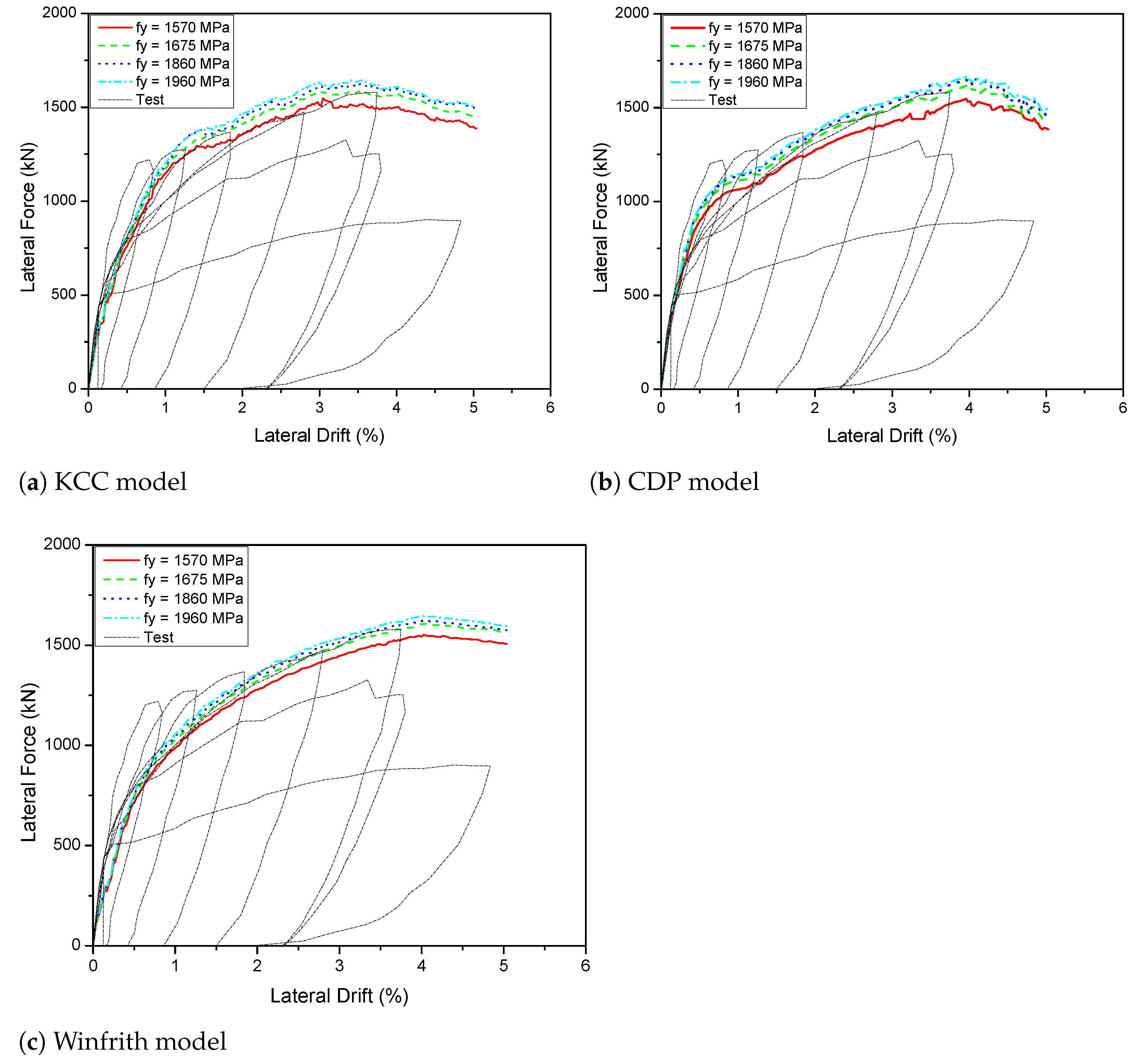
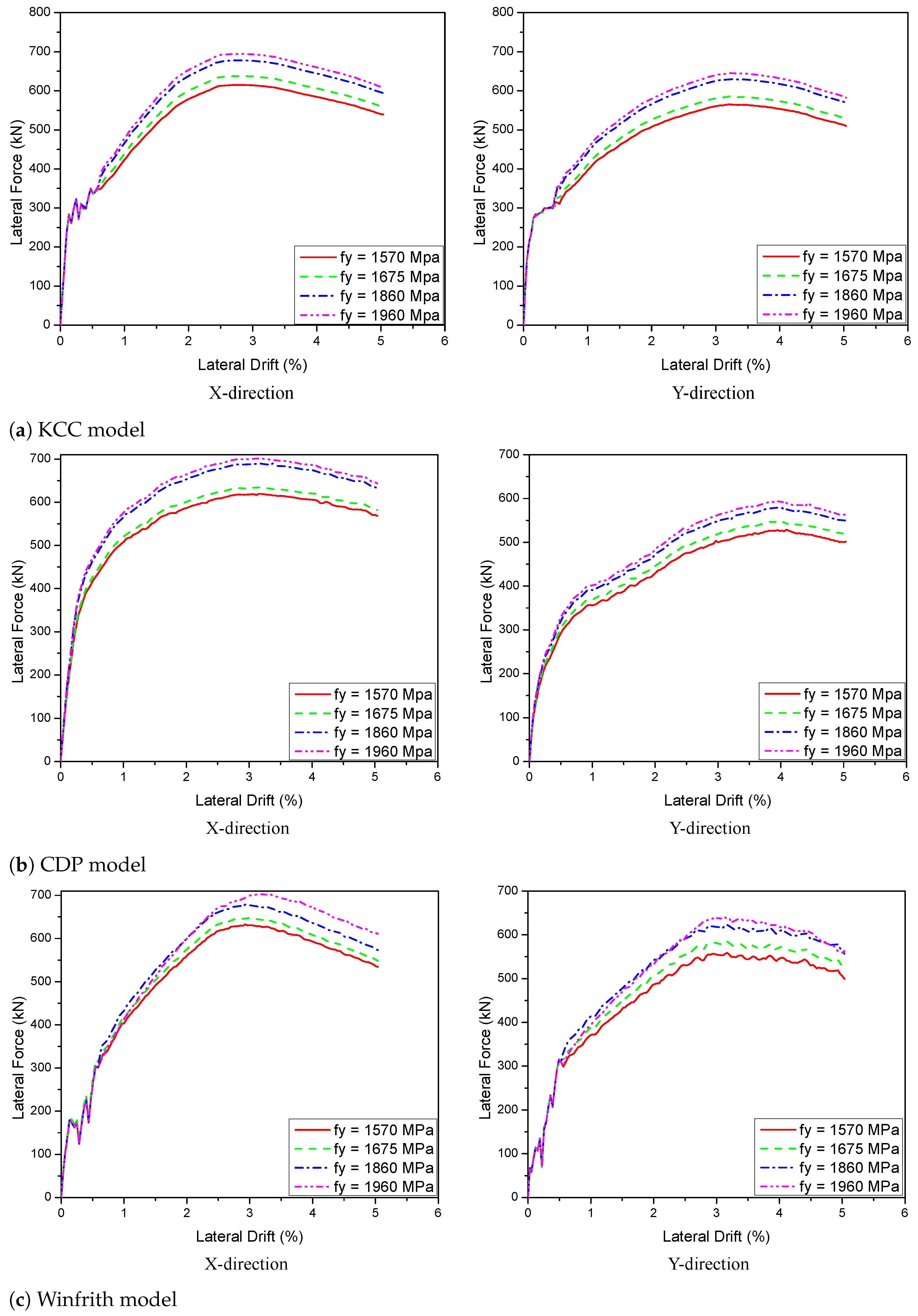
5.1.3. Effect of PT Yield Strength

The pushover curves of specimens with varied $f_y$ are shown in Figure 19. The various parameter ranges were: $f_y=1570$ MPa, $f_y=1675$ MPa, $f_y=1860$ MPa, and $f_y=1960$ MPa. It can be observed that steel strength had the most noticeable effect on the specimen’s peak load when $f_y=1675$ MPa, although it had a minimal effect in the other cases. As a result, when it was raised, the improvement in peak load was not considerable. The lateral strength of the KCC model increased from 1588.3 kN to 1621.9 kN (2.1%) and 1645.8 MPa (3.6%) when the yield strength was increased from 1675 MPa to 1860 MPa and 1960 MPa, respectively. Similarly, since the yield strength was altered from 1675 MPa to 1860 MPa and 1960 MPa, the peak load of the CDP model raised by 2.2% and 2.9%, respectively. The peak load of the Winfrith model, on the other hand, did not alter significantly because the yield strength was changed similarly to the CDP model with 1.1% (from 1675 MPa to 1860 MPa) and 2.4% (from 1675 MPa to 1960 MPa). In order to conduct additional research, the best steel strength value for the PT 2D wall was determined to be 1675 MPa.

Table 8. The different maximum lateral force of the PT yield strength of 2D walls.

Yield Strength	KCC Model		CDP Model		Winfrith Model
	Values (kN)	Errors (%)	Values (kN)	Errors (%)	Values (kN)	Errors (%)
$f_y=1570$ MPa	1520.3	−4.3	1546.8	−4.3	1551.8	−3.4
$f_y=1675$ MPa	1588.34	-	1616.8	-	1606.8	-
$f_y=1860$ MPa	1621.9	2.1	1652.3	2.2	1625.2	1.1
$f_y=1960$ MPa	1645.8	3.6	1665.3	2.9	1646.1	2.4

and Figure 20 show the detailed parameters.

5.2. Effect of PT Bars for PT 3D Wall

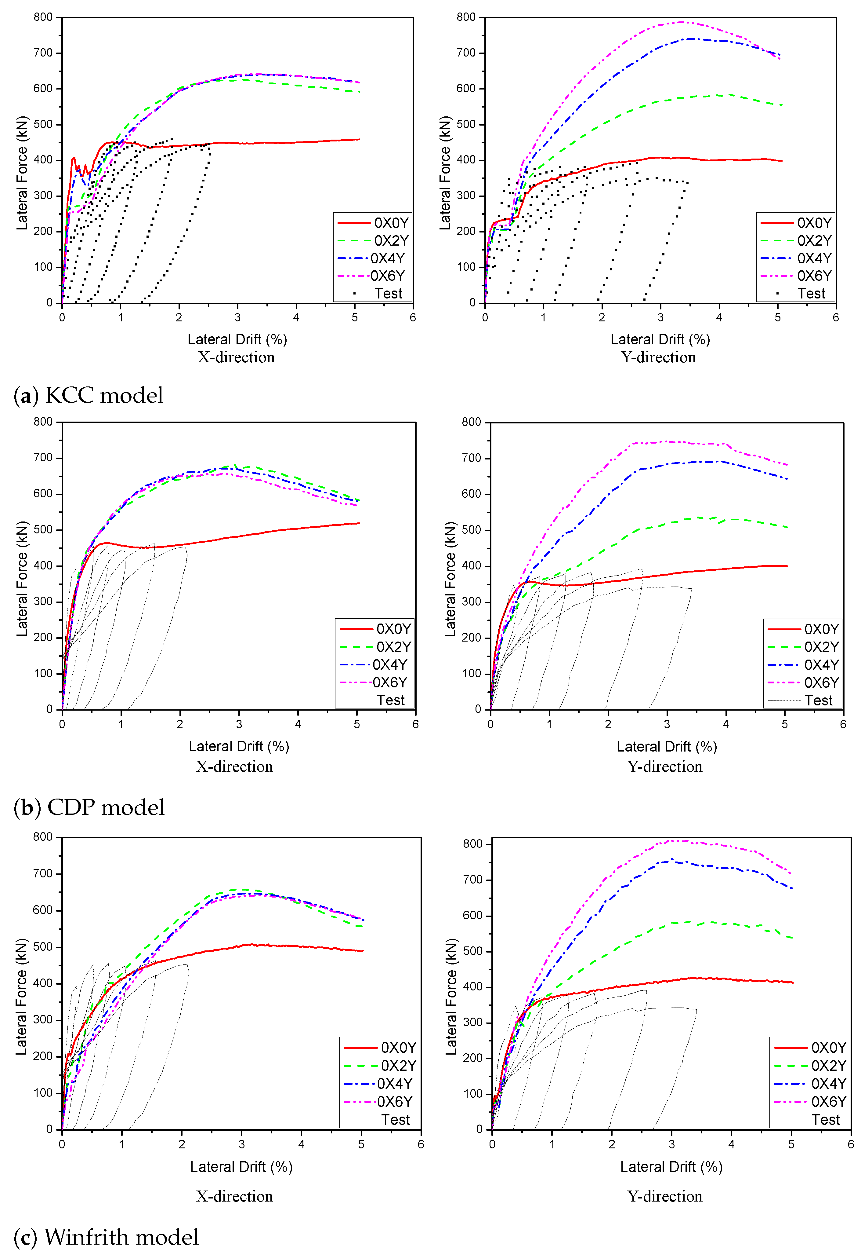
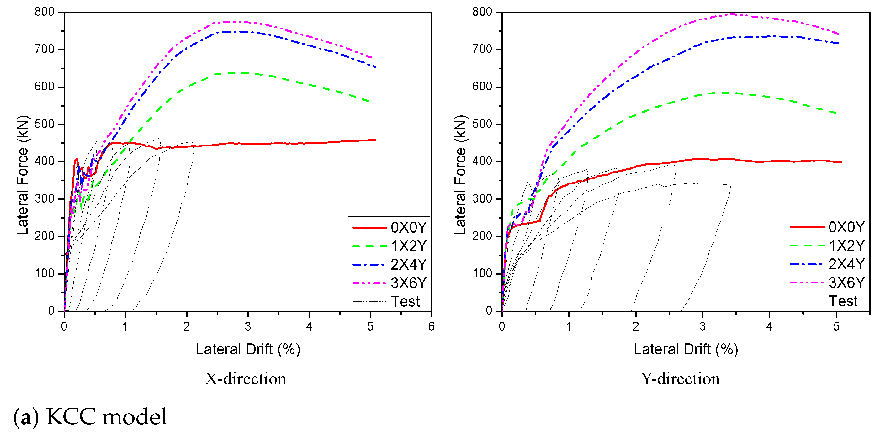
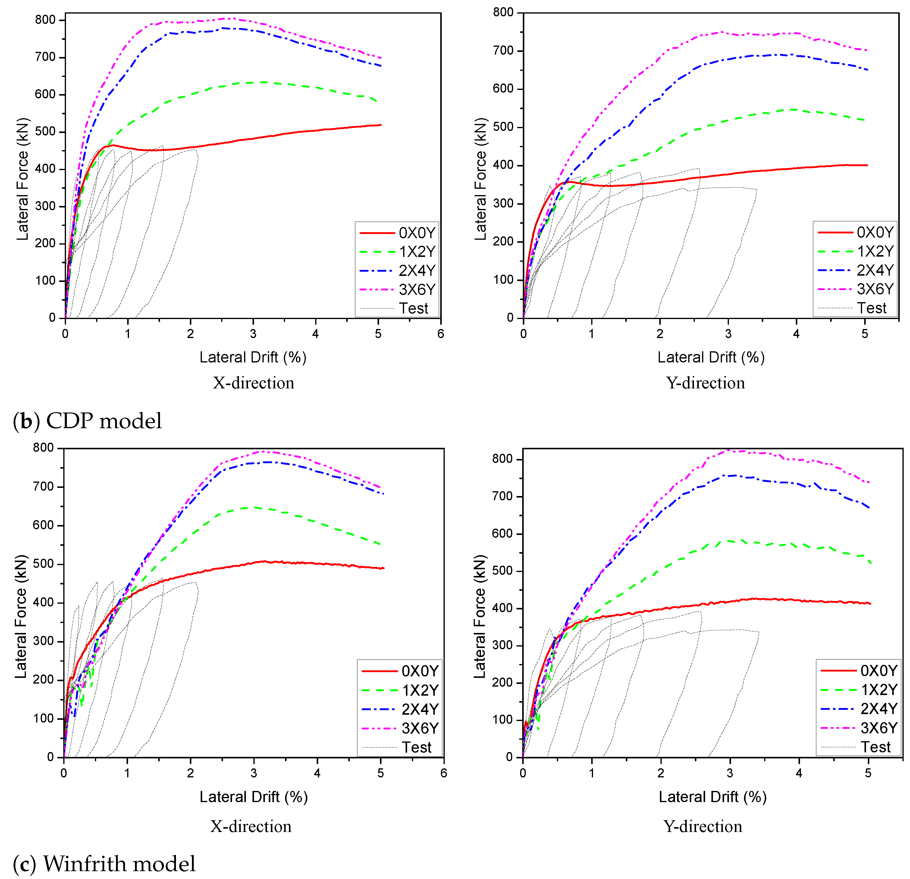
5.2.1. Effect of PT Quantities

The PT quantities were investigated for three scenarios such as -X0Y (0X0Y, 1X0Y, 2X0Y, 3X0Y), 0X-Y (0X0Y, 0X2Y, 0X4Y, 0X6Y), and -X-Y (0X0Y, 1X2Y, 2X4Y, 3X6Y) with diameter of 15.2 mm and yield strength of 1675 MPa, as shown Figure 21. The effect of the PT quantities on the load–displacement curve is illustrated in Figure 22, Figure 23 and Figure 24. In accordance with Figure 22, when the number of PT increased from no PT to one, two, or three PT as shown in Figure 21a, the peak load for the X direction was improved 30.2%, 43.2%, 52.5% for the KCC model and 28.2%, 40.1%, 50.5% for the CDP model, as well as 31.9%, 40.2%, 49.7% for the Winfrith model, respectively. While the peak load of lateral strength for the Y direction did not significantly change. On the other hand, when the number of PT changed from no PT to two, four, or six PT, the peak load of lateral strength for the X direction was improved about 42%, 37% and 37% for the KCC, CDP, and Winfrith models, respectively, as shown in Figure 21b, whereas the peak load for the Y direction was significantly improved. When the number of PT increased from no PT to two PT, the peak load was improved 41.8%, 44.9%, 39.8% for the KCC, CDP, and Winfrith models, respectively. However, when the number of PT was raised from no PT to four PT, the peak load was greatly improved of 79.5%, 79.1%, 81.4% for the KCC, CDP, and Winfrith models, respectively. After that, the peak load was slightly improved with 90.9%, 93.6%, 94.4% for the KCC, CDP, and Winfrith models, respectively, increasing when changing from no PT to six PT as compared previously as shown Figure 23. Finally, when the amount of PT increased from no PT to three, six, and nine PT, as shown in Figure 21c, the peak load of lateral strength for both the X and Y directions was significantly improved. It is noted that the peak load of the X and Y directions was greatly increased for three model such as 66.1% (KCC model), 65.1% (CDP model), 61.5% (Winfrith model) for the X direction as well as 78.5% (KCC model), 79.0% (CDP model), 81.1% (Winfrith model) for the Y direction as the number of PT was changed from none to four, as shown Figure 24. Based on the investigation above, it can be noticed that the scenario of 2X4Y was the optimum choice for the effect of PT quantities for the 3D wall, as shown Figure 25.

Table 9. The different maximum lateral force of PT quantities for the X direction.

PT Quantities	KCC Model		CDP Model		Winfrith Model
	Values (kN)	Errors (%)	Values (kN)	Errors (%)	Values (kN)	Errors (%)
0X0Y	450.9	-	472	-	474.6	-
1X0Y	587.1	30.2	605.1	28.2	626	31.9
2X0Y	645.5	43.2	665	40.1	674.9	42.2
3X0Y	687.9	52.5	710.2	50.5	710.5	49.7
0X2Y	625.9	38.8	652.3	38.2	659.5	38.9
0X4Y	640.8	42.1	650.4	37.8	652.9	37.6
0X6Y	641.9	42.4	648.6	37.4	649	36.7
1X2Y	637.9	41.5	634.3	34.4	649.3	36.8
2X4Y	748.8	66.1	779.5	65.1	766.5	61.5
3X6Y	775.1	71.9	805.4	70.6	792.2	66.9

and

Table 10. The different maximum lateral force of PT quantities for the Y direction.

PT Quantities	KCC Model		CDP Model		Winfrith Model
	Values (kN)	Errors (%)	Values (kN)	Errors (%)	Values (kN)	Errors (%)
3X0Y	420.2	1.8	385.9	−0.2	425.3	1.6
0X2Y	585.1	41.8	560.4	44.9	585.3	39.8
0X0Y	412.7	-	386.8	-	418.8	-
1X0Y	415.3	0.7	384.4	−0.6	420.6	0.4
2X0Y	414.2	0.4	386.1	−0.6	423.2	1.1
0X4Y	740.8	79.5	692.8	79.1	759.9	81.4
0X6Y	787.8	90.9	748.8	93.6	814	94.4
1X2Y	585.5	41.9	548.2	41.7	584.4	39.5
2X4Y	736.5	78.5	692.4	79	758.3	81.1
3X6Y	795.6	92.8	750.3	93.4	826.5	97.3

show the different maximum lateral force of PT quantities for the X and Y directions, respectively.

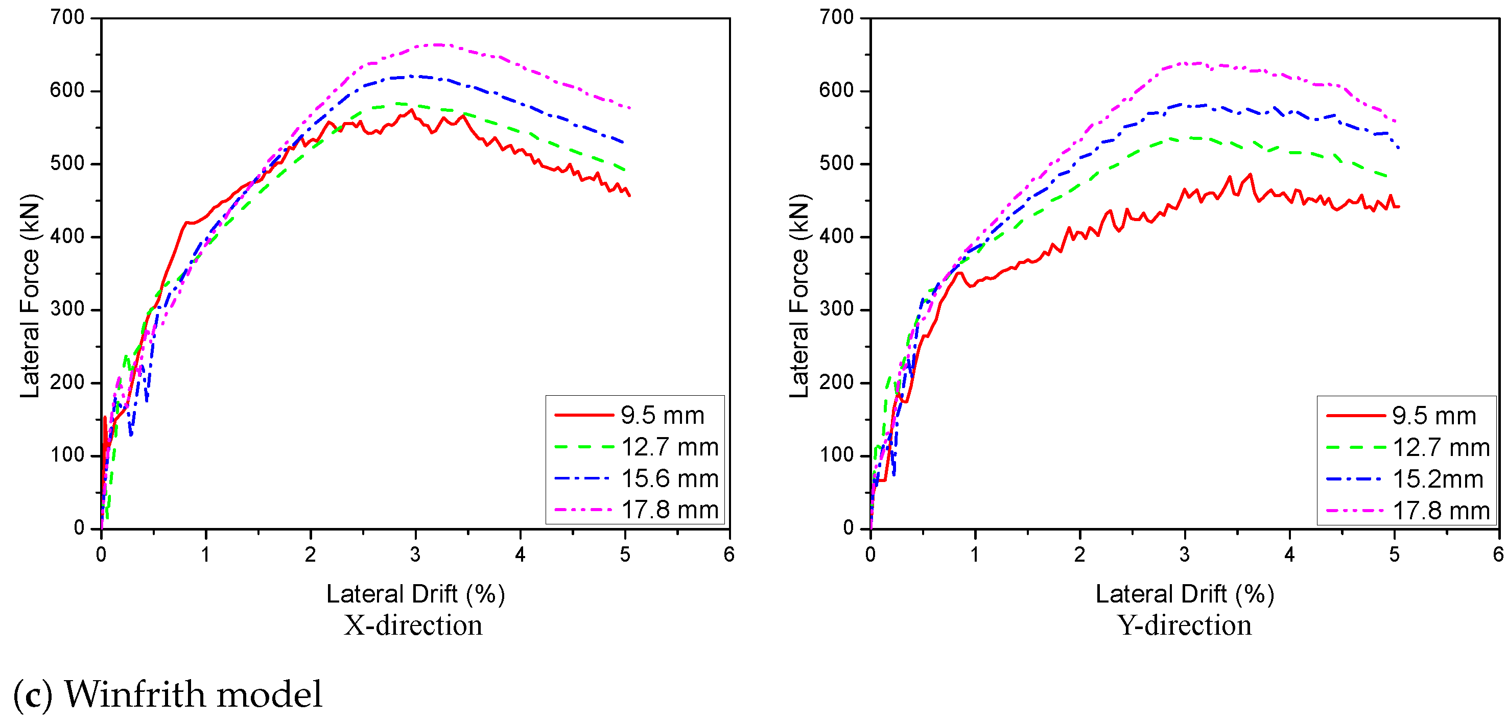
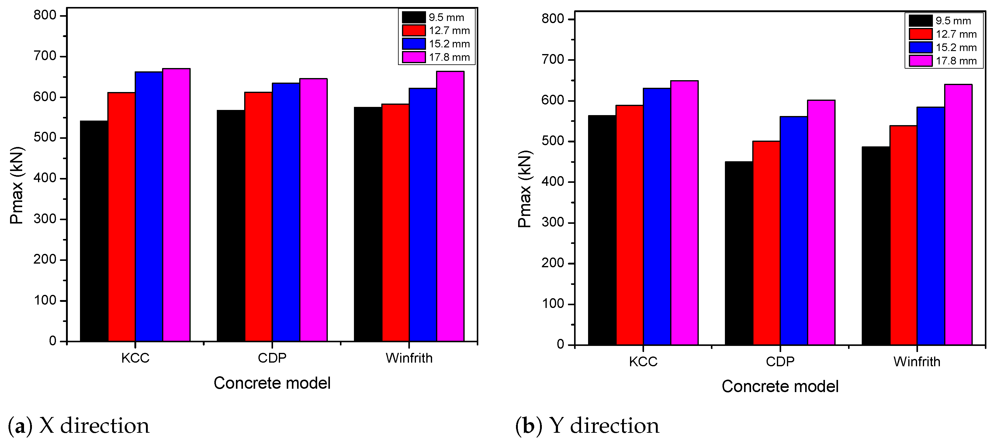
5.2.2. Effect of PT Diameter

There are four scenarios of PT diameter studied to response of the 3D wall behaviour—9.5 mm, 12.7 mm, 15.6 mm, and 17.8 mm. The effect of the PT diameter on the load–displacement curve is shown in Figure 26. In general, the maximum lateral load of the specimen in Figure 26 was improved by changing the PT diameters. According to these plots, when the diameter was improved from 15.2 mm to 17.8 mm, the peak load was increased 1.2% (KCC model), 1.7% (CDP model), 6.7% (Winfrith model) for the X direction and 3.0% (KCC model), 7.2% (CDP model), 9.5% (Winfrith model) for the Y direction. In contrast, concerning the change of diameter from 15.2 mm to 12.7 mm, the peak load decreased 7.7%, 3.5%, and 6.3% for the KCC, CDP, and Winfrith models, respectively, for the X direction, as well as 6.7%, 10.8%, and 7.8% for the KCC, CDP, and Winfrith models, respectively, for the Y direction. Similarly, when the diameter decreased from 15.2 mm to 9.5 mm, the peak load decreased 18.3%, 10.5%, 7.7% for the X direction and 10.7%, 19.8% and 16.8% for the Y direction of the KCC, CDP, and Winfrith models, respectively. This indicated that the 15.2 mm is the best option for enhancing bearing capacity of lateral strength for the 3D wall for three models as shown in Figure 27.

Table 11. The different maximum lateral force of PT diameters for X direction.

PT Diameters	KCC Model		CDP Model		Winfrith Model
	Values (kN)	Errors (%)	Values (kN)	Errors (%)	Values (kN)	Errors (%)
9.5 mm	541.4	−18.3	567.4	−10.5	574.6	−7.7
12.7 mm	611.3	−7.7	612.4	−3.5	583.1	−6.3
15.2 mm	662.4	-	634.3	-	622.2	-
17.8 mm	670.3	1.2	645.4	1.7	663.9	6.7

and

Table 12. The different maximum lateral force of PT diameters for Y direction.

PT Diameters	KCC Model		CDP Model		Winfrith Model
	Values (kN)	Errors (%)	Values (kN)	Errors (%)	Values (kN)	Errors (%)
9.5 mm	562.9	−10.7	449.9	−19.8	486.4	−16.8
12.7 mm	588.5	−6.7	500.6	−10.8	538.6	−7.8
15.2 mm	630.5	-	561.1	-	584.4	-
17.8 mm	649.5	3.0	601.4	7.2	640	9.5

show the details of the parameters.

5.2.3. Effect of the PT Yield Strength

The effect of the PT yield strength on the load–displacement curve is illustrated in Figure 28 for the given examples with the various PT yield strengths ($f_y$ = 1570 MPa, $f_y$ = 1675 MPa, $f_y$ = 1860 MPa and $f_y$ = 1960 MPa), PT quantities of 1X2Y type, and PT diameter of 15.2 mm. When the yield strength was increased 11% (from 1675 MPa to 1860 MPa), the peak load went up 6.3%, 8.8%, 4.5% for the X direction and 7.7%, 5.7%, 6.6% for the Y direction, which were the highest increases of the KCC, CDP and Winfrith models, respectively. This indicated that the most obvious influence of the yield strength of rebars on the peak load of the specimen was the case when $f_y$ = 1860 MPa, whereas it had a minor affect in the others as shown Figure 29.

Table 13. The different maximum lateral force of the PT yield strength for the X direction.

Yield Strength	KCC Model		CDP Model		Winfrith Model
	Values (kN)	Errors (%)	Values (kN)	Errors (%)	Values (kN)	Errors (%)
1570 MPa	615.1	−3.6	619.4	−2.3	632.8	−2.5
1675 MPa	637.9	-	634.3	-	649.3	-
1860 MPa	678.1	6.3	690.3	8.8	678.8	4.5
1960 MPa	694.5	8.9	701.6	10.6	702.6	8.2

and

Table 14. The different maximum lateral force of the PT yield strength for the Y direction.

Yield Strength	KCC Model		CDP Model		Winfrith Model
	Values (kN)	Errors (%)	Values (kN)	Errors (%)	Values (kN)	Errors (%)
1570 MPa	565.3	−3.5	528.9	−3.5	558.7	−4.4
1675 MPa	585.5	-	548.2	-	584.4	-
1860 MPa	630.5	7.7	579.4	5.7	622.8	6.6
1960 MPa	645.3	10.2	593.9	8.3	640	9.5

show the main values of the peak load for the X and Y directions.

6. Conclusions

Models providing for lateral force versus displacement curve represented the behaviour of the RC walls under pushover analysis. The effect of PT bars and behaviour of RC walls were investigated for PT 2D and 3D walls. After that, the effect of PT bars was applied to a 3D wall to predict the response of PT 3D wall behaviour. To analyze the behaviour of several concrete constitutive models, a variety of pushover tests were chosen. Three LS-DYNA concrete models, KCC (MAT072), CDPM (MAT273), and Winfrith (MAT084), were chosen as representations of these constitutive models to evaluate their ability to forecast the seismic response of RC structures. The following list summarizes a number of key conclusions:

1.

All three material models investigated in this study could predict an acceptable peak strength for both PT 2D and 3D walls. The Winfrith model was the best prediction in three models based on the outstanding capability to generate the details of a crack’s location as well as its dimensions. Additionally, not only could it accurately predict the failure position of concrete as compared to the experimental, but the Winfrith model could also identify the regions of maximum flexural stresses in rebars.

2.

The strain rate did not significantly influence the force–displacement relationships for KCC and CDP models but the Winfrith model was converse and the RATE = 1 was appropriate for this model for 2D walls. All three models have a profound effect with the strain rate and the RATE = 1 provided reasonable prediction for the Winfrith model for 3D walls. Because the mesh size of 25 mm and type of element of ELFORM = 1 were suitable for predicting the peak load and minimizing computational time, they were chosen for the numerical simulation.

3.

The number of PT had the greatest influence on lateral strength bearing capacity; yield strength had a negligible effect for PT 2D walls. Based on the numerical simulations, the PT quantity (2X4Y), the PT diameter (15.2 mm) and the yield strength ($f_y$ = 1860 MPa) were selected to efficiently enhance the bearing capacity of lateral strength for PT 3D walls.

References

1. Cheok, G.S. A hybrid reinforced precast frame for seismic regions. PCI J. 1997, 42, 20–32. [Google Scholar]
2. Kurama, Y.; Sause, R.; Pessiki, S.; Lu, L.W. Lateral load behavior and seismic design of unbonded post-tensioned precast concrete walls. Struct. J. 1999, 96, 622–632. [Google Scholar]
3. Twigden, K.M. Dynamic Response of Unbonded Post-Tensioned Concrete Walls for Seismic Resilient Structures. Ph.D. Thesis, University of Auckland, Auckland, New Zealand, 2016. [Google Scholar]
4. Chou, C.C.; Chen, J.H. Analytical model validation and influence of column bases for seismic responses of steel post-tensioned self-centering MRF systems. Eng. Struct. 2011, 33, 2628–2643. [Google Scholar] [CrossRef]
5. Kalliontzis, D.; Sritharan, S. Seismic behavior of unbonded post-tensioned precast concrete members with thin rubber layers at the jointed connection. PCI J. 2021, 66, 60–76. [Google Scholar] [CrossRef]
6. Christopoulos, C.; Filiatrault, A.; Uang, C.M.; Folz, B. Posttensioned energy dissipating connections for moment-resisting steel frames. J. Struct. Eng. 2002, 128, 1111–1120. [Google Scholar] [CrossRef]
7. Newcombe, M.; Pampanin, S.; Buchanan, A.; Palermo, A. Section analysis and cyclic behavior of post-tensioned jointed ductile connections for multi-story timber buildings. J. Earthq. Eng. 2008, 12, 83–110. [Google Scholar] [CrossRef]
8. Kurama, Y.C. Seismic design of partially post-tensioned precast concrete walls. PCI J. 2005, 50, 100. [Google Scholar] [CrossRef]
9. Aaleti, S.; Sritharan, S. A simplified analysis method for characterizing unbonded post-tensioned precast wall systems. Eng. Struct. 2009, 31, 2966–2975. [Google Scholar] [CrossRef]
10. Ou, Y.C.; Chiewanichakorn, M.; Aref, A.J.; Lee, G.C. Seismic performance of segmental precast unbonded posttensioned concrete bridge columns. J. Struct. Eng. 2007, 133, 1636–1647. [Google Scholar] [CrossRef]
11. Xu, G.; Li, A. Seismic performance and design approach of unbonded post-tensioned precast sandwich wall structures with friction devices. Eng. Struct. 2020, 204, 110037. [Google Scholar] [CrossRef]
12. Hallquist, J.O. LS-DYNA Keyword User’s Manual; Livermore Software Technology Corporation: Troy, MI, USA, 2007; Volume 970, pp. 299–800. [Google Scholar]
13. Riedel, W. 10 years RHT: A review of concrete modelling and hydrocode applications. In Predictive Modeling of Dynamic Processes; Springer: Berlin/Heidelberg, Germany, 2009; pp. 143–165. [Google Scholar]
14. Xu, J.; Lu, Y. A comparative study of modelling RC slab response to blast loading with two typical concrete material models. Int. J. Prot. Struct. 2013, 4, 415–432. [Google Scholar] [CrossRef] [Green Version]
15. Tu, Z.; Lu, Y. Evaluation of typical concrete material models used in hydrocodes for high dynamic response simulations. Int. J. Impact Eng. 2009, 36, 132–146. [Google Scholar] [CrossRef]
16. Bao, X.; Li, B. Residual strength of blast damaged reinforced concrete columns. Int. J. Impact Eng. 2010, 37, 295–308. [Google Scholar] [CrossRef]
17. Zhang, C.; Abedini, M.; Mehrmashhadi, J. Development of pressure-impulse models and residual capacity assessment of RC columns using high fidelity Arbitrary Lagrangian-Eulerian simulation. Eng. Struct. 2020, 224, 111219. [Google Scholar] [CrossRef]
18. Abedini, M.; Zhang, C. Performance assessment of concrete and steel material models in ls-dyna for enhanced numerical simulation, a state of the art review. Arch. Comput. Methods Eng. 2021, 28, 2921–2942. [Google Scholar] [CrossRef]
19. Mutalib, A.A.; Tawil, N.M.; Baharom, S.; Abedini, M. Failure probabilities of FRP strengthened RC column to blast loads. J. Teknol. 2013, 65, 135–141. [Google Scholar] [CrossRef] [Green Version]
20. Asgarpoor, M.; Gharavi, A.; Epackachi, S. Investigation of various concrete materials to simulate seismic response of RC structures. Structures 2021, 29, 1322–1351. [Google Scholar] [CrossRef]
21. Mohammed, T.A.; Parvin, A. Evaluating damage scale model of concrete materials using test data. Adv. Concr. Constr. 2013, 1, 289. [Google Scholar] [CrossRef] [Green Version]
22. Kazaz, l.; Yakut, A.; Polat, G. Numerical Simulation of Dynamic Shear Wall Tests: A Benchmark Study. Comput. Struct. 2006, 84, 549–562. [Google Scholar] [CrossRef]
23. Morales, E.; Filiatrault, A.; Aref, A. Sustainable and low cost room seismic isolation for essential care units of hospitals in developing countries. In Proceedings of the 16th World Conference on Earthquake Engineering, Santiago, Chile, 9–13 January 2017. [Google Scholar]
24. Sanja, H.; Yves, M.; Urs, B.; Tadeusz, S.; Dimitrios, Z. Beyond Design Seismic Capacity Of Squat RC Shear Walls: Lessons Learnt From Phase 2 Of The CASH Benchmark Exercise Using LS-DYNA. In Proceedings of the Transactions, SMiRT-25, Charlotte, NC, USA, 4–9 August 2019. [Google Scholar]
25. Bojanowski, C.; Kulak, R.F. Seismic and Traffic Load Modeling on Cable Stayed Bridge. Technical Report. 2011. Available online: https://trid.trb.org/view/1092530 (accessed on 2 May 2022).
26. Coleman, D.K. Evaluation of Concrete Modeling in LS-DYNA for Seismic Application. Ph.D. Thesis, University of Texas at Austin, Austin, TX, USA, 2016. [Google Scholar]
27. Sturt, R.; Avanes, C.; Muriithi, B.; Bernardi, M.; Huang, Y. A masonry material model for seismic analysis in LS-DYNA: Implementation and validation. In Proceedings of the 16th European Conference on Earthquake Engineering, Thessaloniki, Greece, 18–21 June 2018. [Google Scholar]
28. Bocciarelli, M.; Barbieri, G. A numerical procedure for the pushover analysis of masonry towers. Soil Dyn. Earthq. Eng. 2017, 93, 162–171. [Google Scholar] [CrossRef]
29. Chomchuen, P.; Boonyapinyo, V. Incremental dynamic analysis with multi-modes for seismic performance evaluation of RC bridges. Eng. Struct. 2017, 132, 29–43. [Google Scholar] [CrossRef]
30. Fanaie, N.; Ezzatshoar, S. Studying the seismic behavior of gate braced frames by incremental dynamic analysis (IDA). J. Constr. Steel Res. 2014, 99, 111–120. [Google Scholar] [CrossRef]
31. Taghinezhad, R.; Taghinezhad, A.; Mahdavifar, V.; Soltangharaei, V. Seismic Vulnerability Assessment of Coupled Wall RC Structures. Int. J. Sci. Eng. Appl. 2018, 7, 1–7. [Google Scholar] [CrossRef]
32. Pan, X.; Zheng, Z.; Wang, Z. Estimation of floor response spectra using modified modal pushover analysis. Soil Dyn. Earthq. Eng. 2017, 92, 472–487. [Google Scholar] [CrossRef]
33. Taghinezhad, R.; Taghinezhad, A.; Mahdavifar, V.; Soltangharaei, V. Numerical Investigation of Deflection Amplification Factor in Moment Resisting Frames Using Nonlinear Pushover Analysis. Int. J. Innov. Eng. Sci. 2017, 2, 1–7. [Google Scholar]
34. Seible, F.; LaRovere, H.; Kingsley, G. Nonlinear analysis of reinforced concrete masonry shear wall structures—Monotonic loading. Mason. Soc. J. 1990, 9. [Google Scholar]
35. Lotfi, H.R.; Shing, P.B. Interface model applied to fracture of masonry structures. J. Struct. Eng. 1994, 120, 63–80. [Google Scholar] [CrossRef]
36. Mehrabi, A.B.; Shing, P.B. Finite element modeling of masonry-infilled RC frames. J. Struct. Eng. 1997, 123, 604–613. [Google Scholar] [CrossRef]
37. Damoni, C.; Belletti, B.; Esposito, R. Numerical prediction of the response of a squat shear wall subjected to monotonic loading. Eur. J. Environ. Civ. Eng. 2014, 18, 754–769. [Google Scholar] [CrossRef]
38. Li, H.; Shi, G. Material modeling of concrete for the numerical simulation of steel plate reinforced concrete panels subjected to impacting loading. J. Eng. Mater. Technol. 2017, 139, 021011. [Google Scholar] [CrossRef]
39. Hong, J.; Fang, Q.; Chen, L.; Kong, X. Numerical predictions of concrete slabs under contact explosion by modified K&C material model. Constr. Build. Mater. 2017, 155, 1013–1024. [Google Scholar]
40. Xu, M.; Wille, K. Calibration of K&C concrete model for UHPC in LS-DYNA. In Advanced Materials Research; Trans Tech Publications Ltd.: Bach, Switzerland, 2015; Volume 1081, pp. 254–259. [Google Scholar]
41. Kong, X.; Fang, Q.; Li, Q.; Wu, H.; Crawford, J.E. Modified K&C model for cratering and scabbing of concrete slabs under projectile impact. Int. J. Impact Eng. 2017, 108, 217–228. [Google Scholar]
42. Deng, Y.; Tuan, C.Y. Design of concrete-filled circular steel tubes under lateral impact. ACI Struct. J. 2013, 110, 691. [Google Scholar]
43. Pham, T.M.; Hao, Y.; Hao, H. Sensitivity of impact behaviour of RC beams to contact stiffness. Int. J. Impact Eng. 2018, 112, 155–164. [Google Scholar] [CrossRef]
44. Wu, J.; Liu, X.; Zhou, H.; Li, L.; Liu, Z. Experimental and numerical study on soft-hard-soft (SHS) cement based composite system under multiple impact loads. Mater. Des. 2018, 139, 234–257. [Google Scholar] [CrossRef] [Green Version]
45. Malvar, L.J.; Crawford, J.E. Dynamic Increase Factors for Concrete; Technical Report; Naval Facilities Engineering Service Center: Port Hueneme, CA, USA, 1998. [Google Scholar]
46. Grassl, P.; Jirásek, M. Damage-plastic model for concrete failure. Int. J. Solids Struct. 2006, 43, 7166–7196. [Google Scholar] [CrossRef] [Green Version]
47. Grassl, P.; Xenos, D.; Nyström, U.; Rempling, R.; Gylltoft, K. CDPM2: A damage-plasticity approach to modelling the failure of concrete. Int. J. Solids Struct. 2013, 50, 3805–3816. [Google Scholar] [CrossRef] [Green Version]
48. Broadhouse, B.; Neilson, A. Modelling Reinforced Concrete Structures in DYNA3D; Technical Report; UKAEA Atomic Energy Establishment: Abingdon, UK, 1987. [Google Scholar]
49. Pakiding, L.; Pessiki, S.; Sause, R.; Rivera, M. Lateral load response of unbonded post-tensioned cast-in-place concrete walls. In Structures Congress 2015; American Society of Civil Engineers: Reston, VA, USA, 2015; pp. 1338–1349. [Google Scholar]
50. Beyer, K.; Dazio, A.; Priestley, M. Quasi-static cyclic tests of two U-shaped reinforced concrete walls. J. Earthq. Eng. 2008, 12, 1023–1053. [Google Scholar] [CrossRef]
51. LS-DYNA. Keyword Users Manual-Volume II: Material Models; Livermore Software Technology Corporation: Livermore, CA, USA, 2016. [Google Scholar]
52. Abu-Odeh, A. Modeling and simulation of bogie impacts on concrete bridge rails using LS-DYNA. In Proceedings of the 10th International LS-DYNA Users Conference, Dearborn, MI, USA, 8–10 June 2008; Volume 1, pp. 9–20. [Google Scholar]
53. Bhargawa, A.; Roddis, W.K.; Marzougui, D.; Mohan, P.K. Analysis of Extended End-Plate Connections Under Cyclic Loading Using the LS-DYNA Implicit Solver. In Proceedings of the 9th International LS-DYNA Conference, Detroit, MI, USA, 4–6 June 2006. [Google Scholar]
54. Abedini, M.; Mutalib, A.A.; Raman, S.N.; Akhlaghi, E.; Mussa, M.H.; Ansari, M. Numerical investigation on the non-linear response of reinforced concrete (RC) columns subjected to extreme dynamic loads. J. Asian Sci. Res. 2017, 7, 86–98. [Google Scholar] [CrossRef] [Green Version]
55. Lu, G.; Li, X.; Wang, K. A numerical study on the damage of projectile impact on concrete targets. Comput. Concr. 2012, 9, 21–33. [Google Scholar] [CrossRef]
56. Majidi, L.; Usefi, N.; Abbasnia, R. Numerical study of RC beams under various loading rates with LS-DYNA. J. Cent. South Univ. 2018, 25, 1226–1239. [Google Scholar] [CrossRef]
Figure 1. Strain softening behavior for CDP model.
Sustainability 14 06141 g001
Figure 2. Crack strain softening response.
Sustainability 14 06141 g002
Figure 3. Reinforced detials, geometric and FE model for PT 2D walls.
Sustainability 14 06141 g003
Figure 4. Predicted load–displacement curve with various mesh sizes for PT 2D wall.
Sustainability 14 06141 g004aSustainability 14 06141 g004b
Figure 5. Predicted load–displacement curve with different element types for PT 2D walls.
Sustainability 14 06141 g005
Figure 6. Relative time of calculation versus element type.
Sustainability 14 06141 g006
Figure 7. Predicted load–displacement curve with strain rate for PT 2D wall.
Sustainability 14 06141 g007aSustainability 14 06141 g007b
Figure 8. The structural damage reproduced from the finite element model for the PT 2D wall. (a) KCC model. (b) CDP model. (c) Winfrith model.
Sustainability 14 06141 g008
Figure 9. Reinforced details, geometric and FE model for 3D walls.
Sustainability 14 06141 g009
Figure 10. Predicted load–displacement curve with various mesh sizes for 3D wall.
Sustainability 14 06141 g010
Figure 11. Predicted load–displacement curve with different element types for 3D walls.
Sustainability 14 06141 g011aSustainability 14 06141 g011b
Figure 12. Predicted load–displacement curve with strain rate for 3D walls.
Sustainability 14 06141 g012aSustainability 14 06141 g012b
Figure 13. The structural damage reproduced from the finite element model for the 3D wall. (a) KCC model. (b) CDP model. (c) Winfrith model.
Sustainability 14 06141 g013aSustainability 14 06141 g013b
Figure 14. Predicted load–displacement curve with PT quantities for 2D wall.
Sustainability 14 06141 g014
Figure 15. Predicted load–displacement curve with PT quantities for PT 2D wall.
Sustainability 14 06141 g015
Figure 16. The maximum lateral force of PT quantities of PT 2D wall.
Sustainability 14 06141 g016
Figure 17. Predicted load–displacement curve with various diameters for PT 2D wall.
Sustainability 14 06141 g017aSustainability 14 06141 g017b
Figure 18. The maximum lateral force of PT diameters of PT 2D wall.
Sustainability 14 06141 g018
Figure 19. Predicted load–displacement curve with the PT yield strength.
Sustainability 14 06141 g019
Figure 20. The maximum lateral force of the PT yield strength for PT 2D wall.
Sustainability 14 06141 g020
Figure 21. The FE model of the PT quantites for PT 3D wall.
Sustainability 14 06141 g021
Figure 22. Predicted load–displacement curve with PT quantities of -X0Y for PT 3D wall.
Sustainability 14 06141 g022
Figure 23. Predicted load–displacement curve with PT quantities of 0X-Y for PT 3D wall.
Sustainability 14 06141 g023
Figure 24. Predicted load–displacement curve with PT quantities of -X-Y for PT 3D wall.
Sustainability 14 06141 g024aSustainability 14 06141 g024b
Figure 25. The maximum lateral force of PT quantities for PT 3D wall.
Sustainability 14 06141 g025
Figure 26. Predicted load–displacement curve with various PT diameters for PT 3D wall.
Sustainability 14 06141 g026aSustainability 14 06141 g026b
Figure 27. The peak load of PT diameters for PT 3D wall.
Sustainability 14 06141 g027
Figure 28. Predicted load–displacement curve with the various PT yield strengths for PT 3D wall.
Sustainability 14 06141 g028
Figure 29. The peak load of the PT yield strength for the PT 3D wall.
Sustainability 14 06141 g029