Figure 1.
Proposed drag reduction technique on an intercity bus.
Figure 1.
Proposed drag reduction technique on an intercity bus.
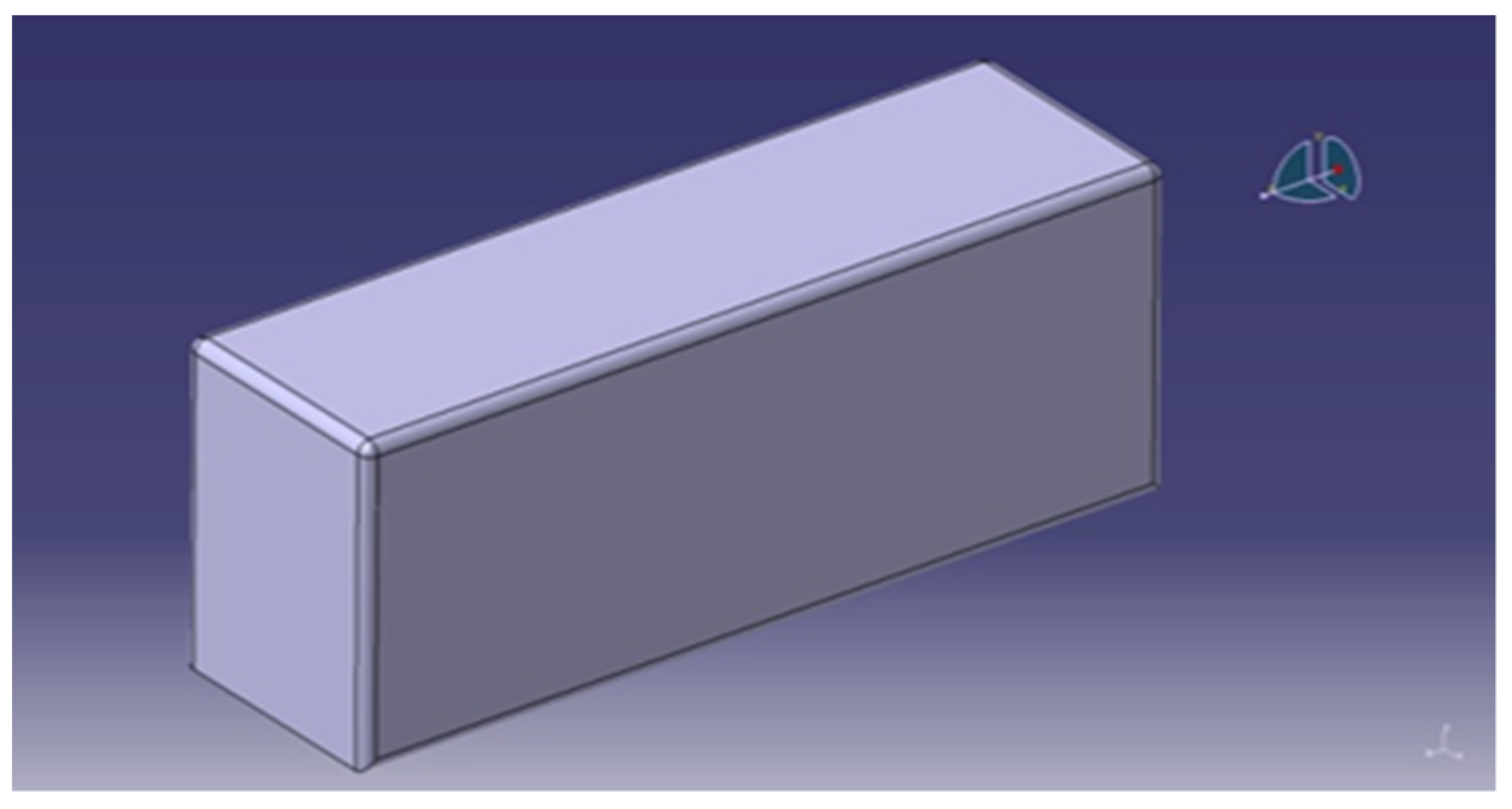
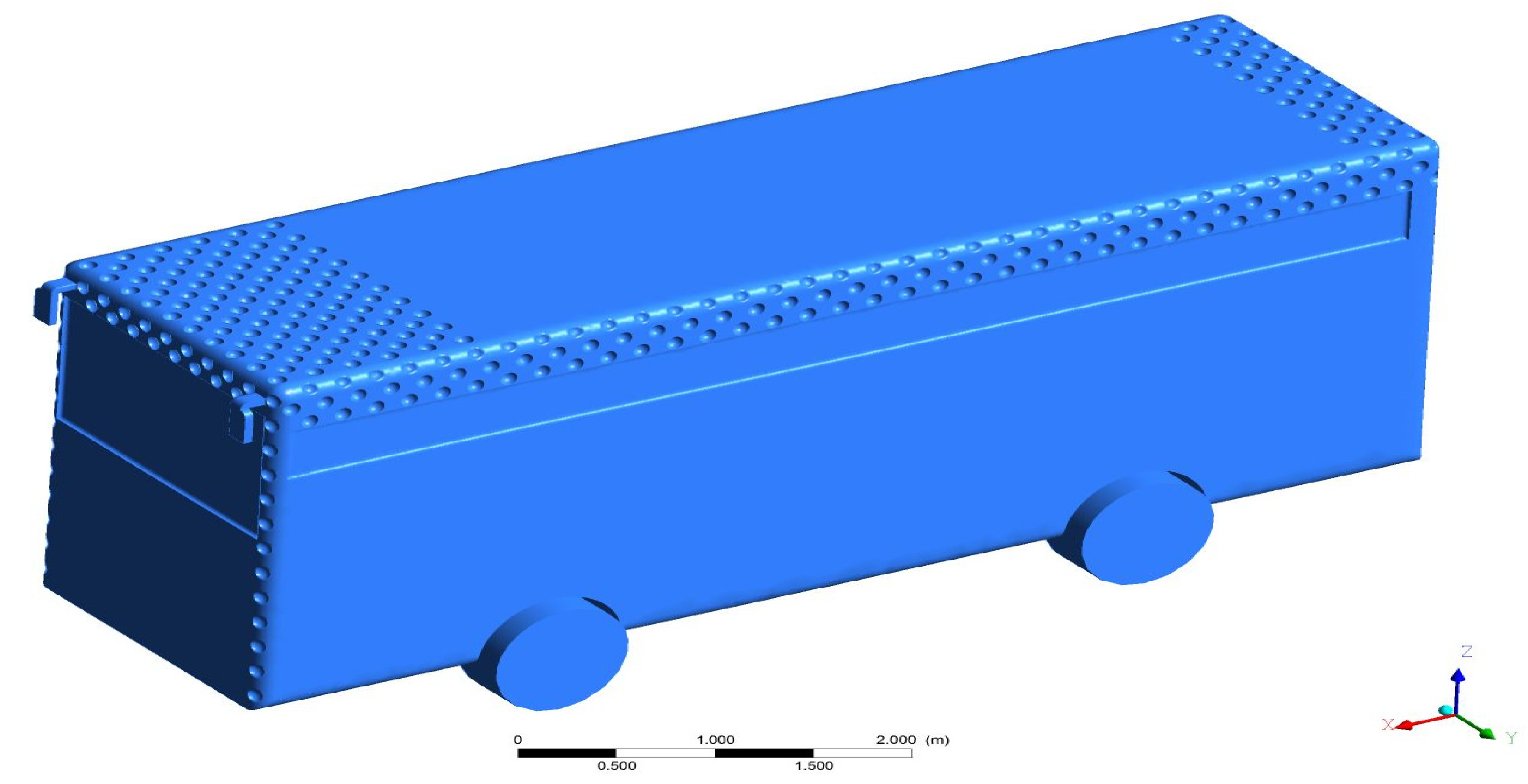
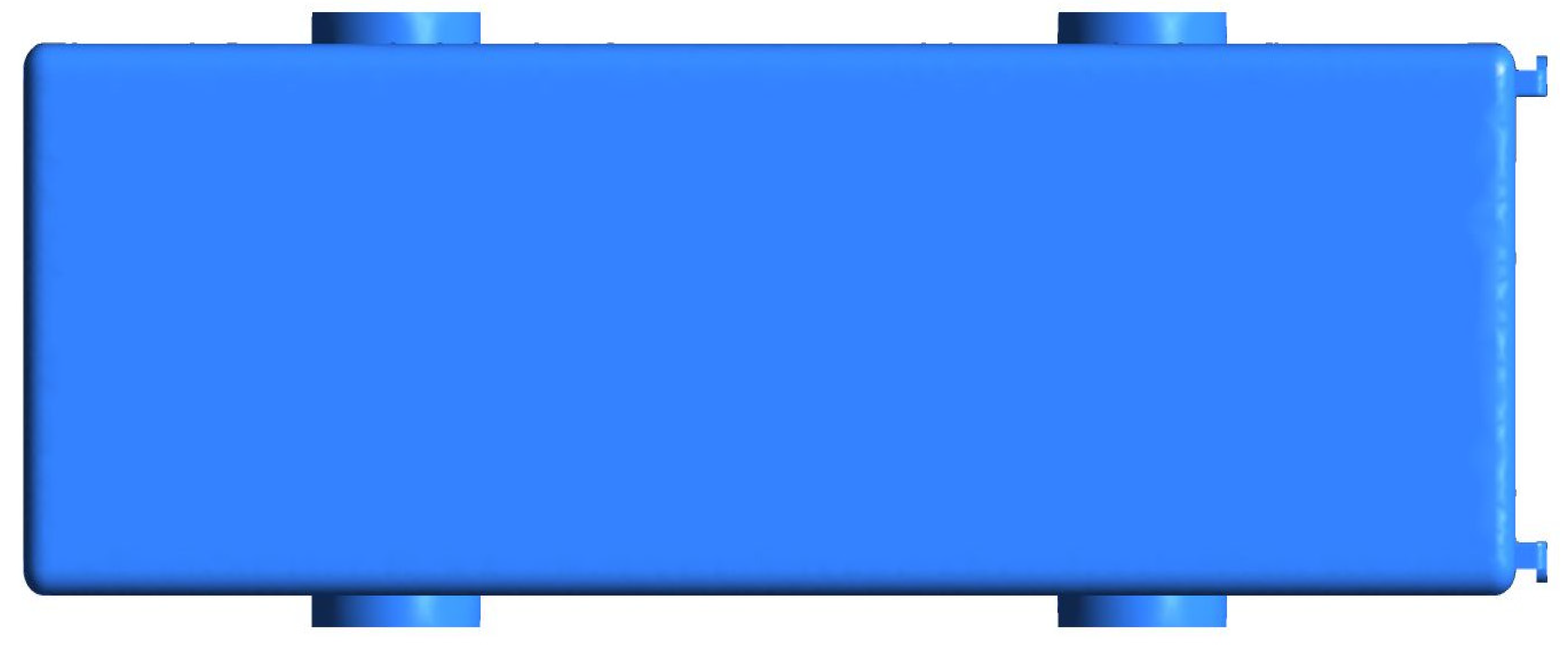
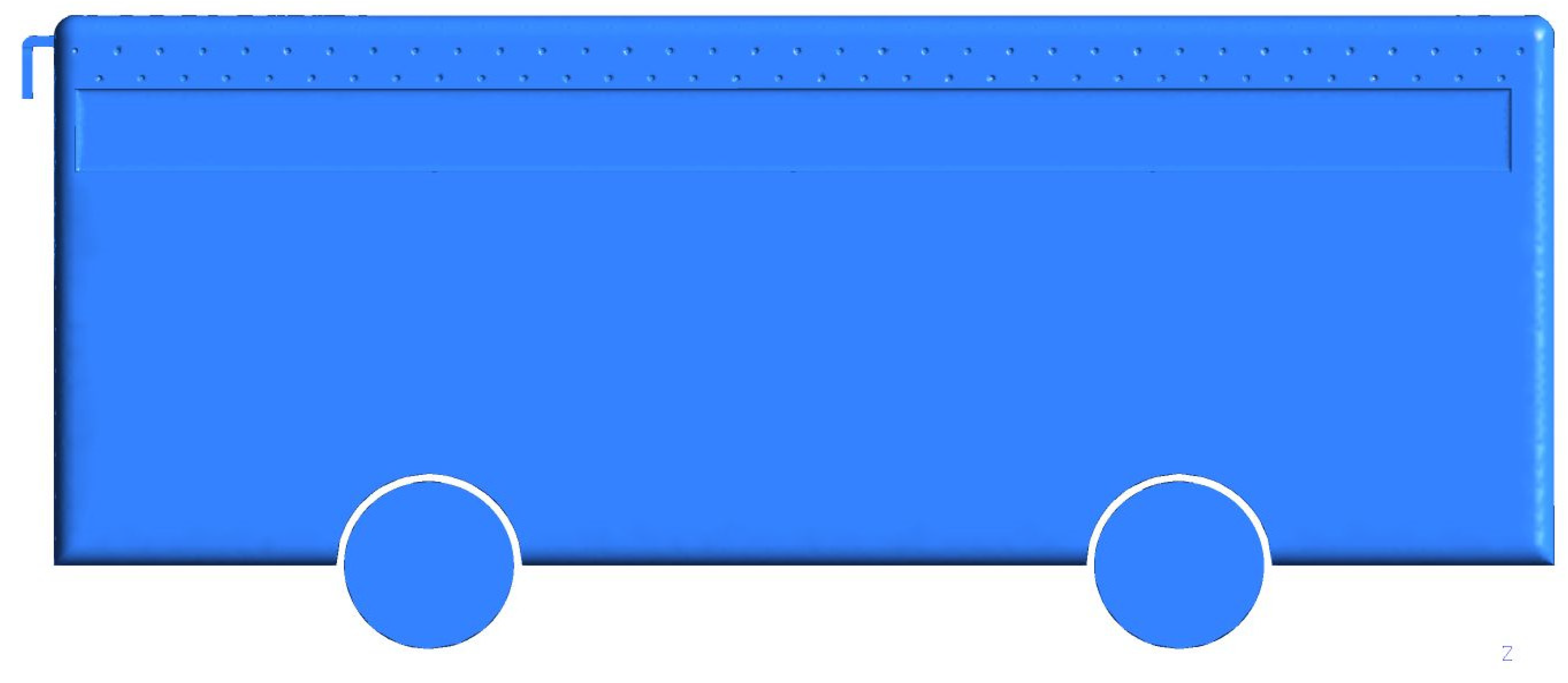
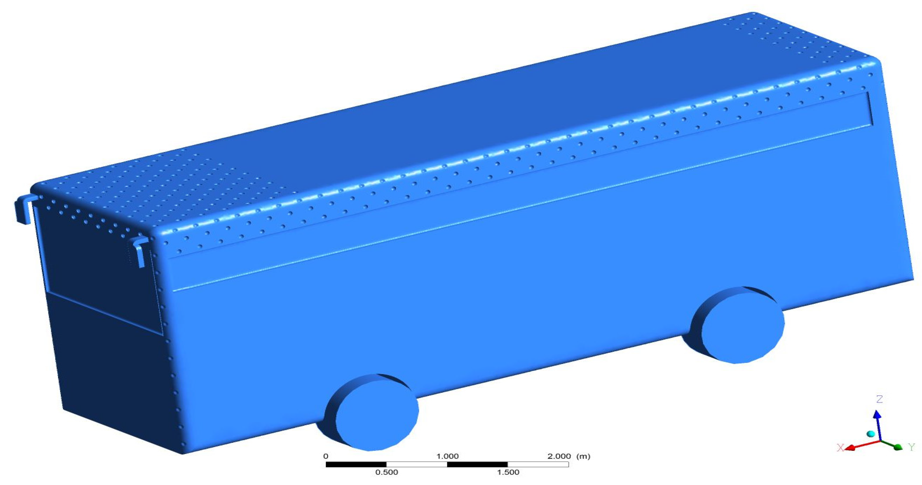
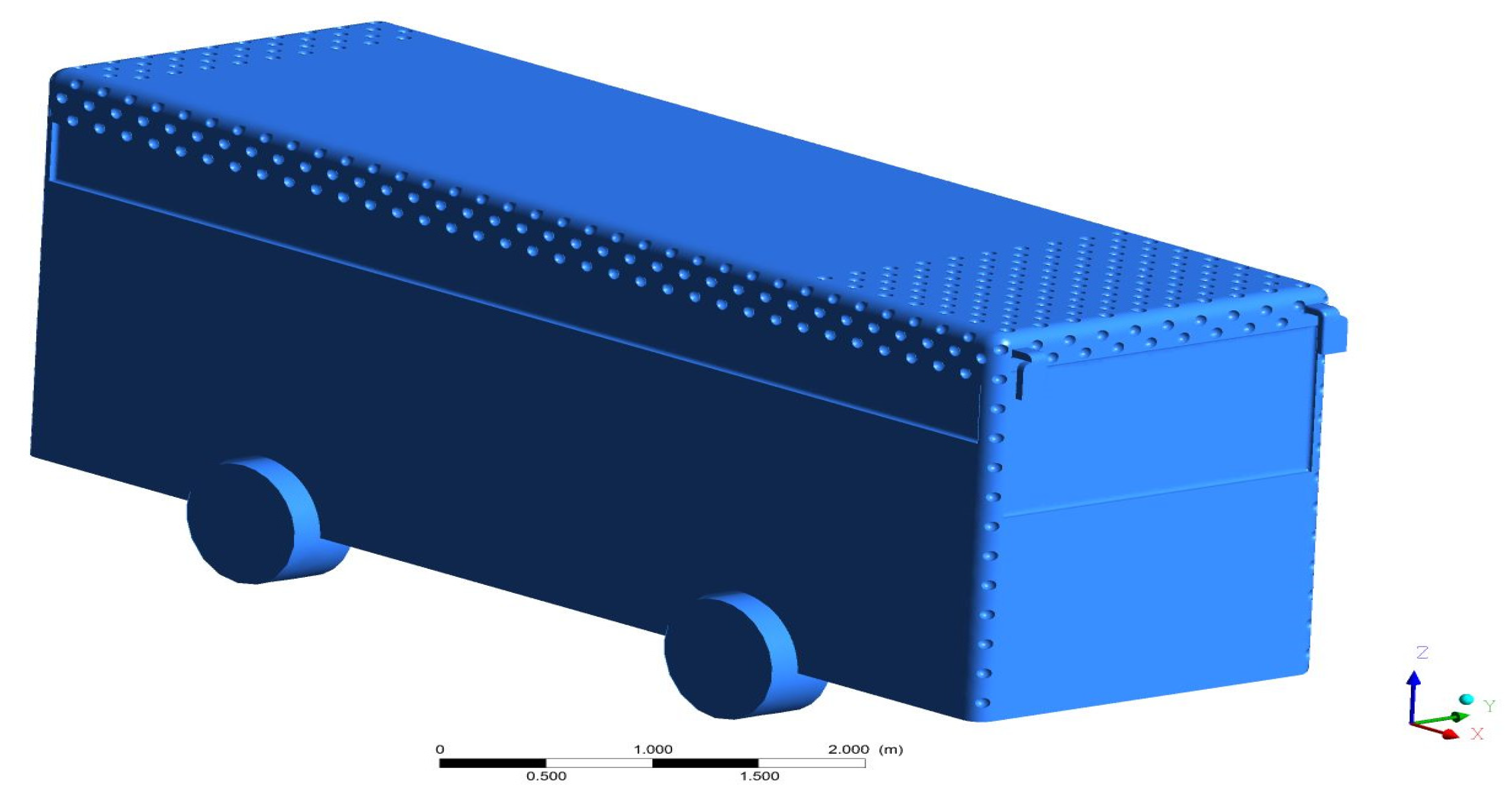
Figure 2.
A typical view of the base design of the intercity bus’s main body.
Figure 2.
A typical view of the base design of the intercity bus’s main body.
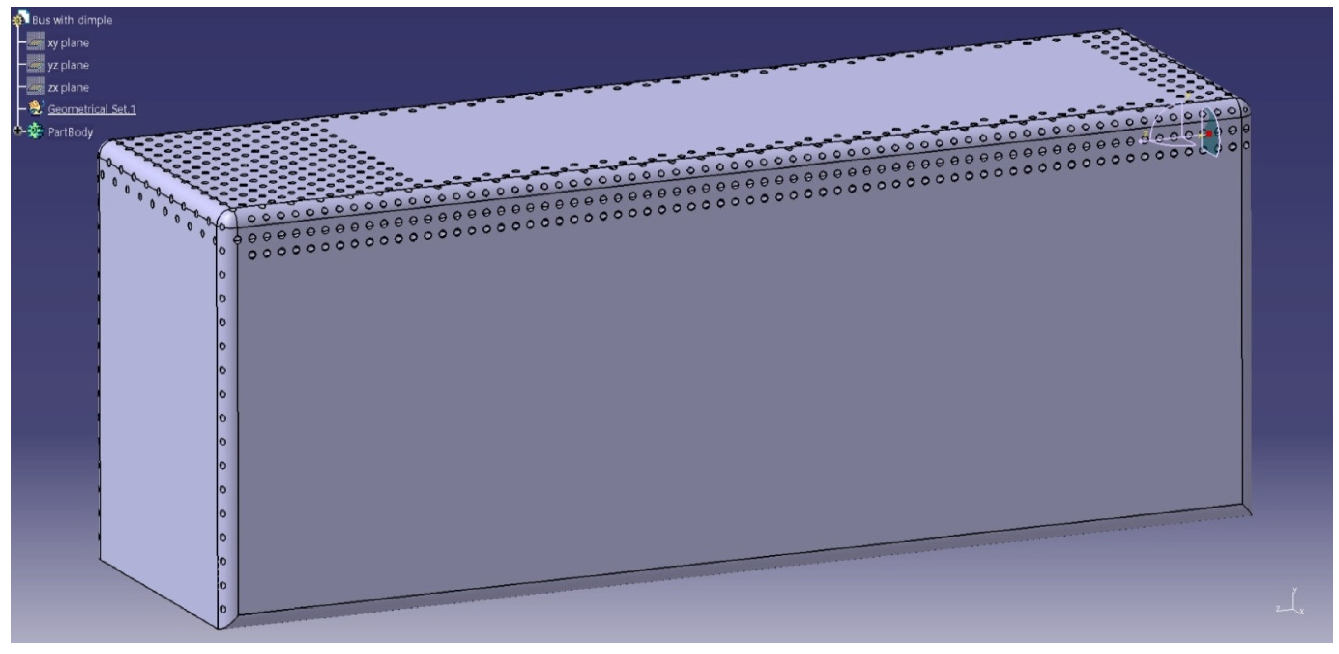
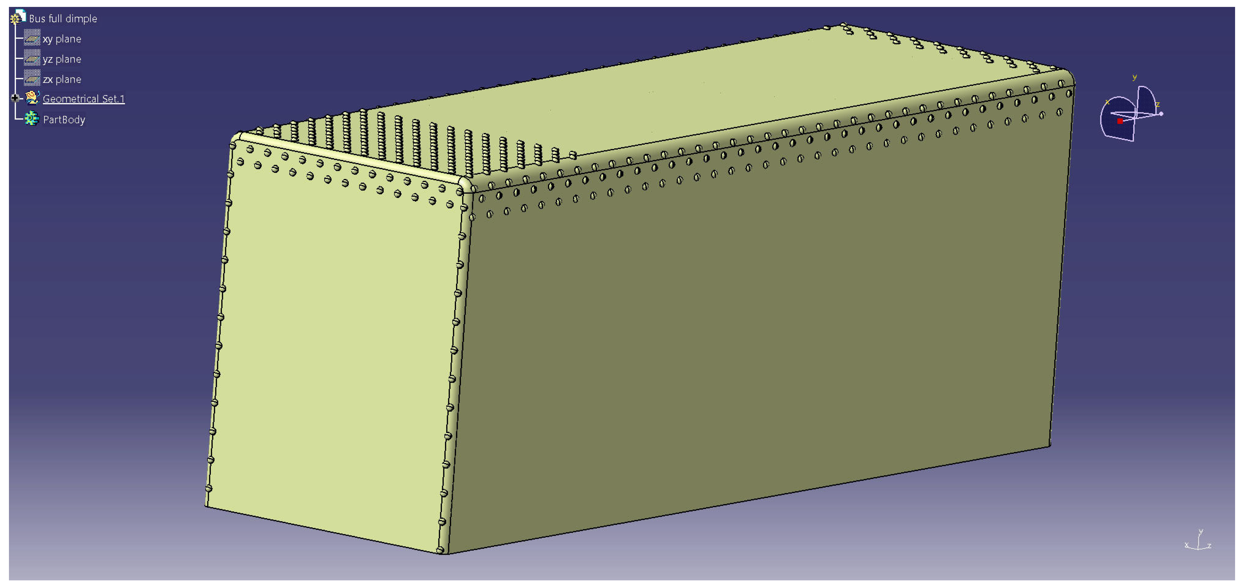
Figure 3.
An isometric view of the main body of an intercity bus loaded with many dimples located partially on the top and side faces.
Figure 3.
An isometric view of the main body of an intercity bus loaded with many dimples located partially on the top and side faces.
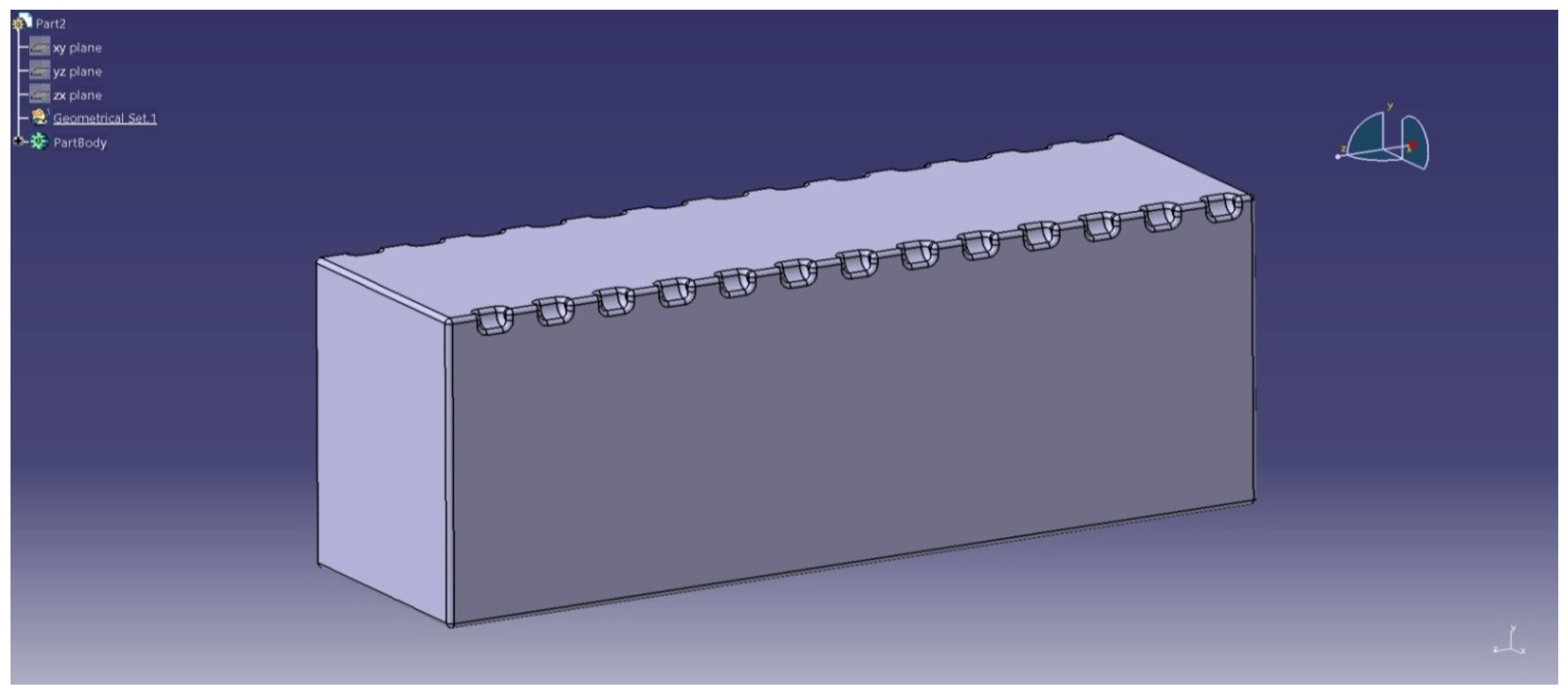
Figure 4.
An isometric view of the main body of an intercity bus loaded with a medium number of inverted dimples located partially on the top and side faces.
Figure 4.
An isometric view of the main body of an intercity bus loaded with a medium number of inverted dimples located partially on the top and side faces.
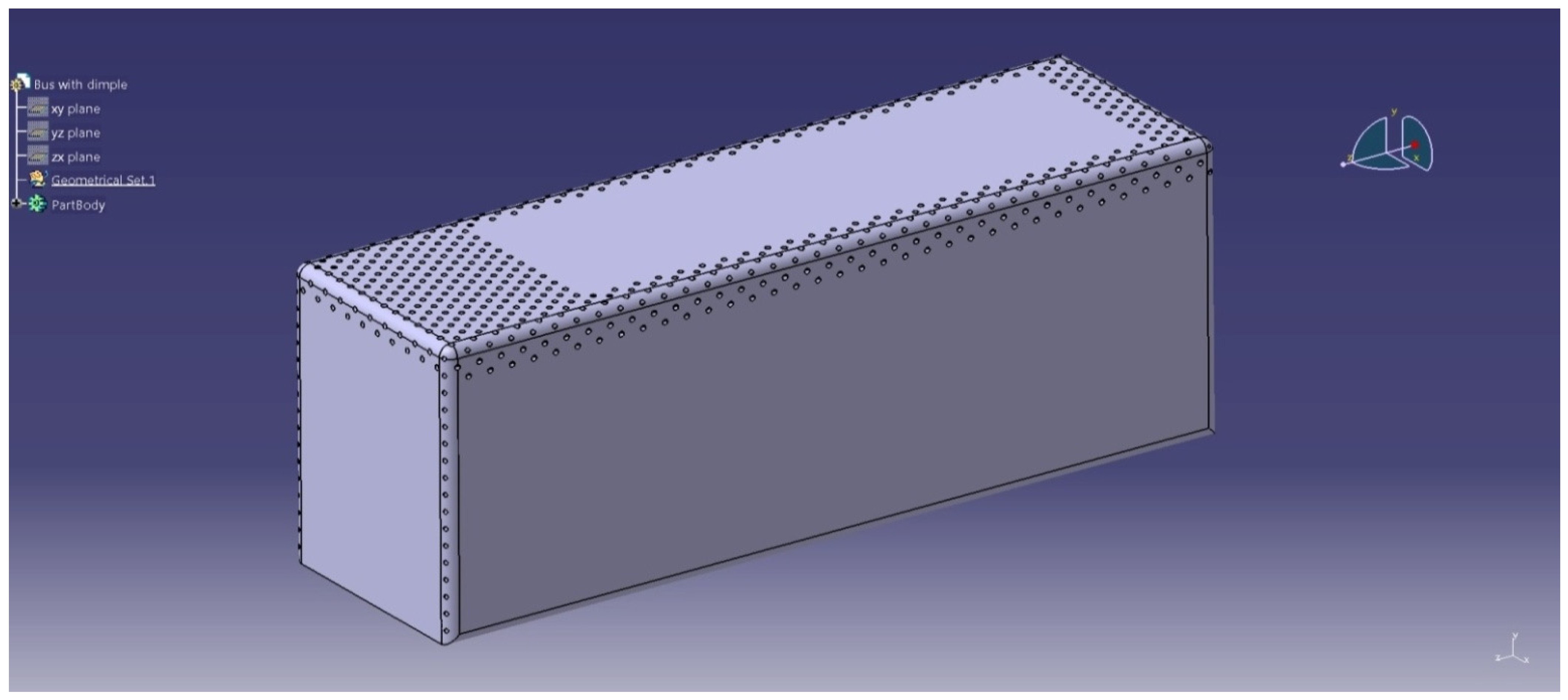
Figure 5.
An isometric view of the main body of an intercity bus loaded with a medium number of dimples located partially on the top and side faces.
Figure 5.
An isometric view of the main body of an intercity bus loaded with a medium number of dimples located partially on the top and side faces.
Figure 6.
An isometric view of the main body of an intercity bus loaded with a small number of square cuts located on the side faces in the longitudinal direction.
Figure 6.
An isometric view of the main body of an intercity bus loaded with a small number of square cuts located on the side faces in the longitudinal direction.
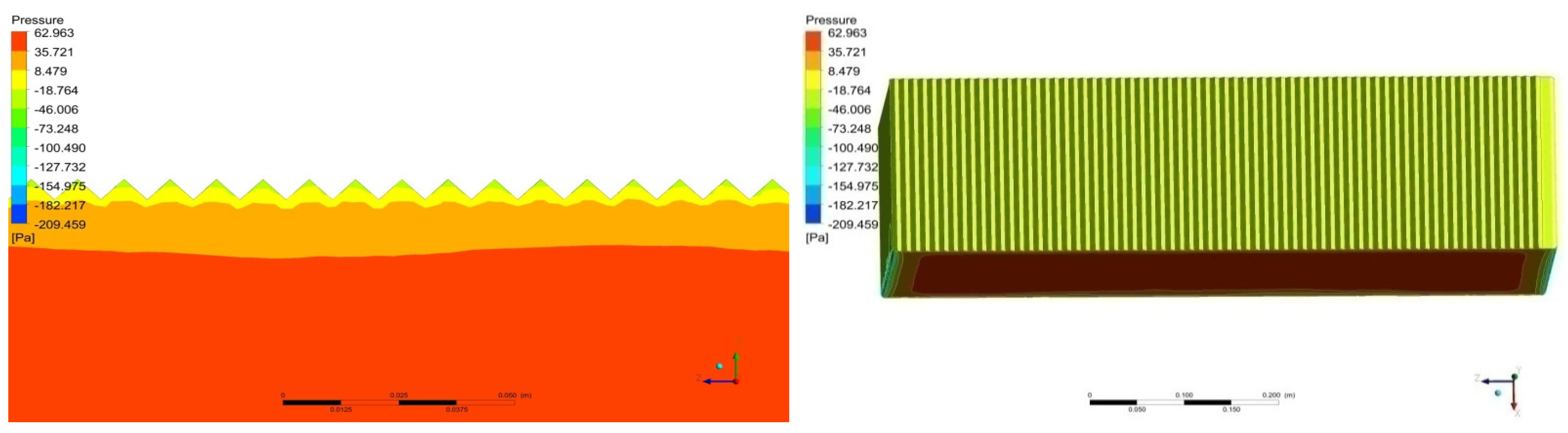
Figure 7.
An isometric view of the main body of an intercity bus loaded with a high number of 10 mm gap-based fins on the top faces.
Figure 7.
An isometric view of the main body of an intercity bus loaded with a high number of 10 mm gap-based fins on the top faces.
Figure 8.
An isometric view of the main body of an intercity bus loaded with a medium number of 20 mm gap-based fins on the top faces.
Figure 8.
An isometric view of the main body of an intercity bus loaded with a medium number of 20 mm gap-based fins on the top faces.
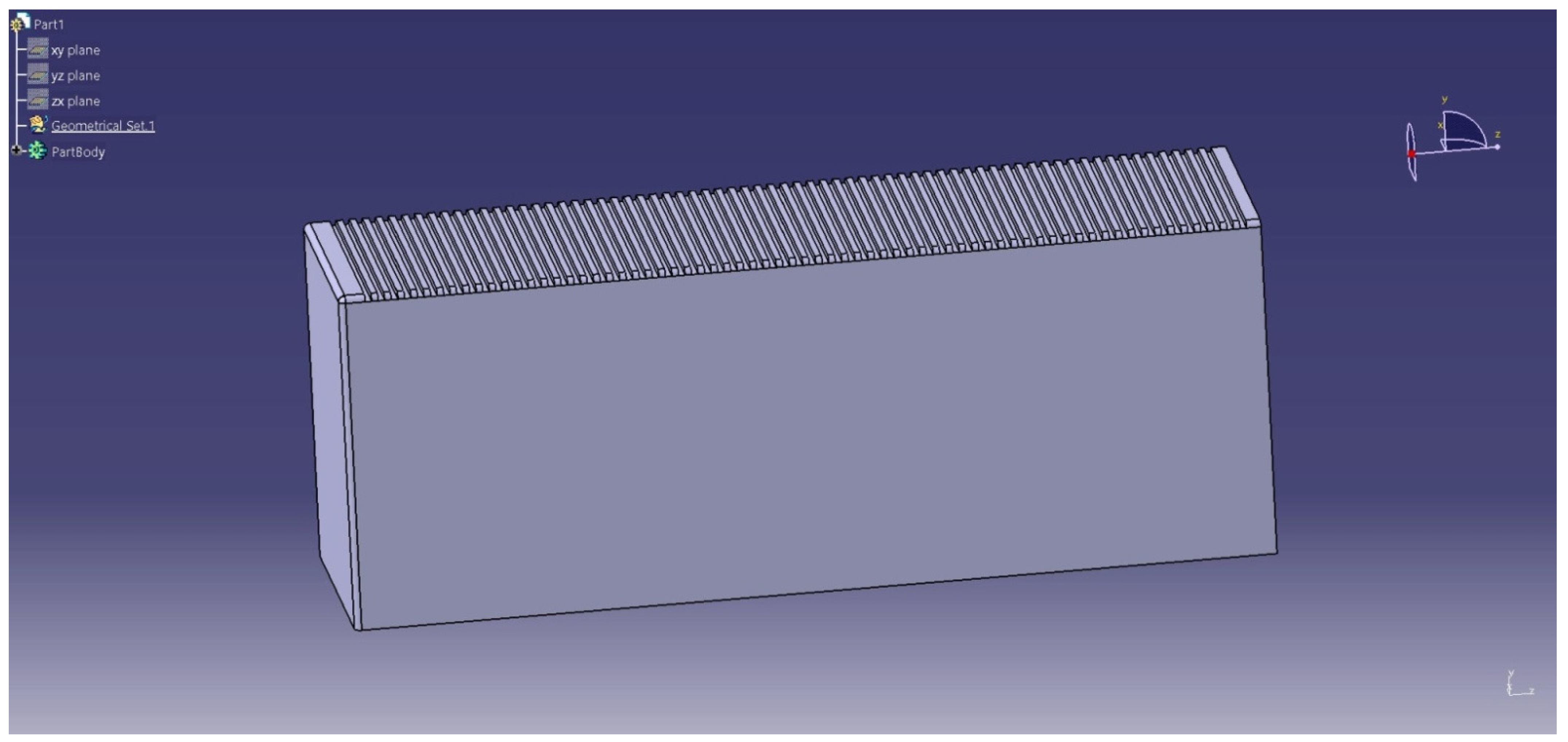
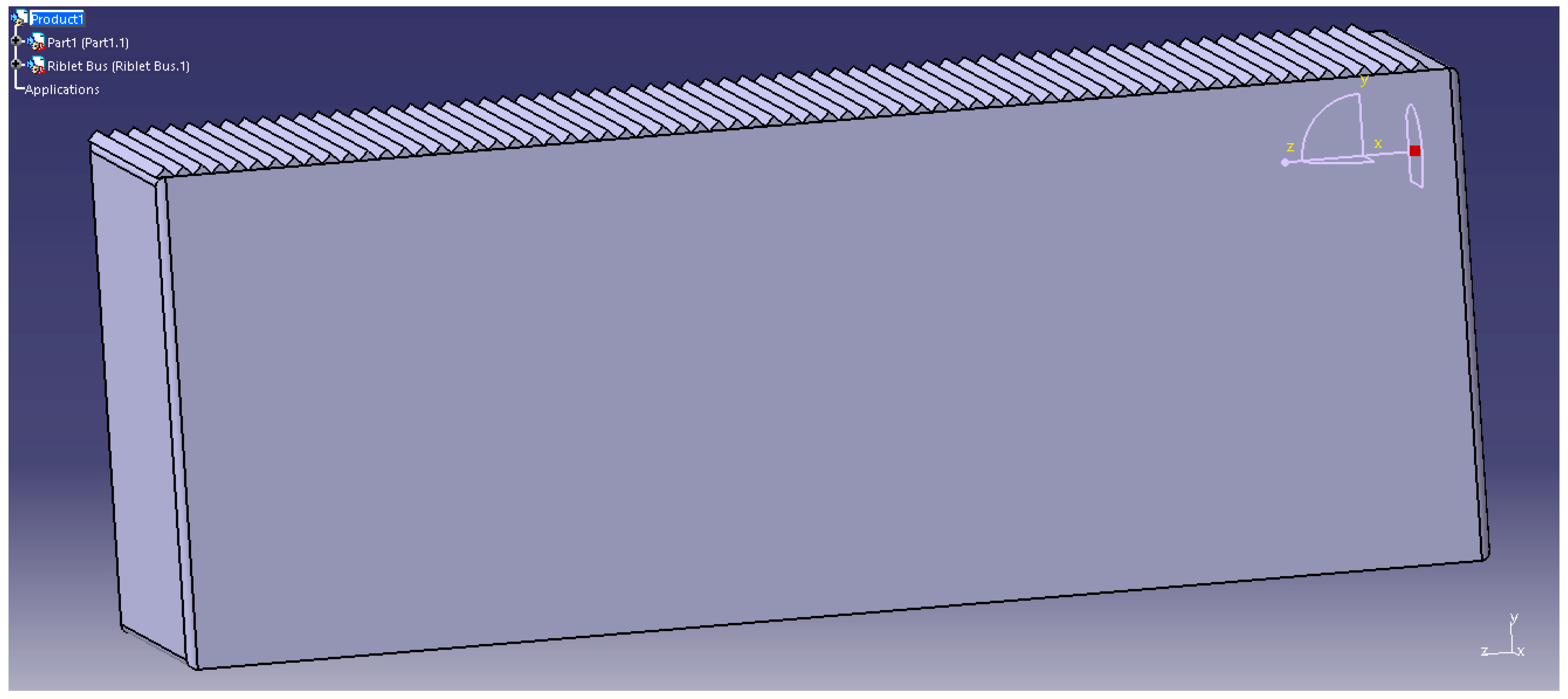
Figure 9.
An isometric view of the main body of an intercity bus loaded with a high number of riblets on the top face.
Figure 9.
An isometric view of the main body of an intercity bus loaded with a high number of riblets on the top face.
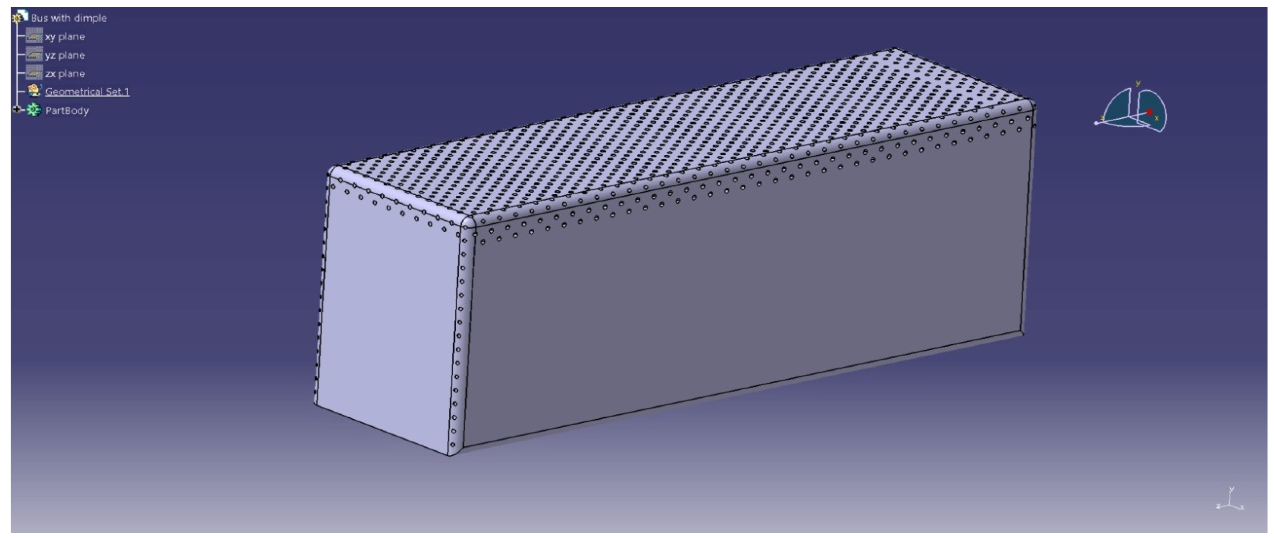
Figure 10.
An isometric view of the main body of an intercity bus loaded with a medium number of dimples located completely on the top and partially on the side faces.
Figure 10.
An isometric view of the main body of an intercity bus loaded with a medium number of dimples located completely on the top and partially on the side faces.
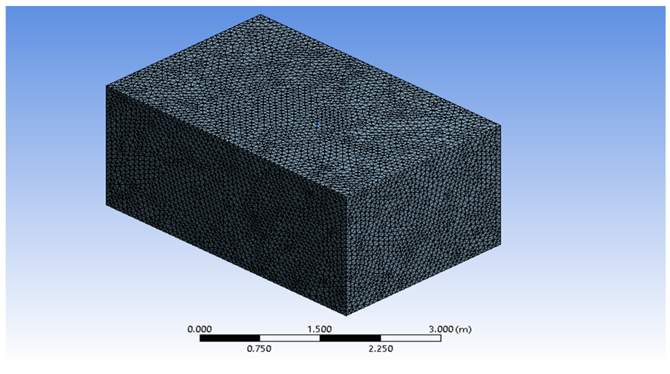
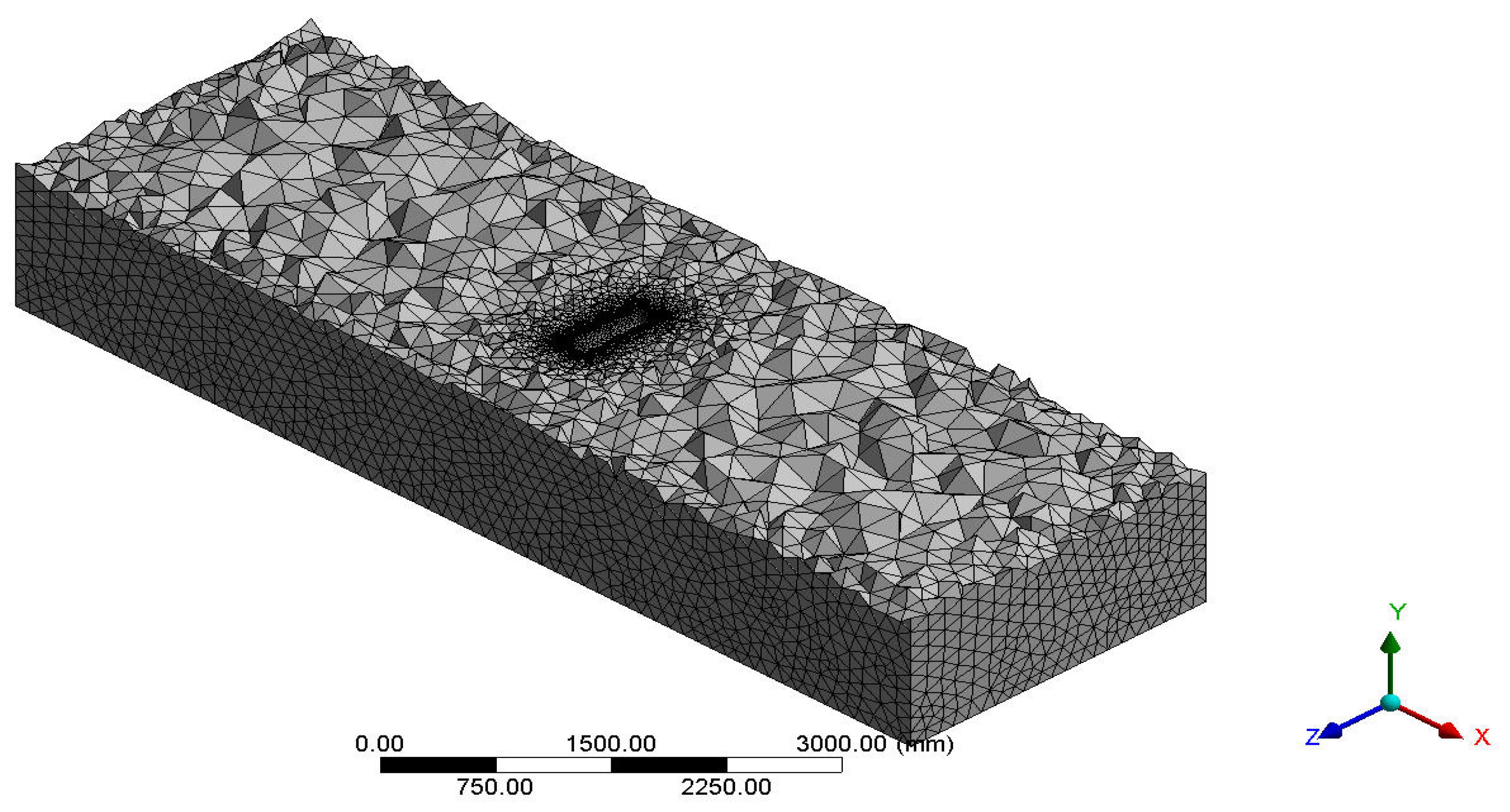
Figure 11.
Solid model view of the discretized structure of the base bus model—curvature-based unstructured mesh.
Figure 11.
Solid model view of the discretized structure of the base bus model—curvature-based unstructured mesh.
Figure 12.
Wireframe model view of the discretized structure—fine curvature with face mesh setup on model VI.
Figure 12.
Wireframe model view of the discretized structure—fine curvature with face mesh setup on model VI.
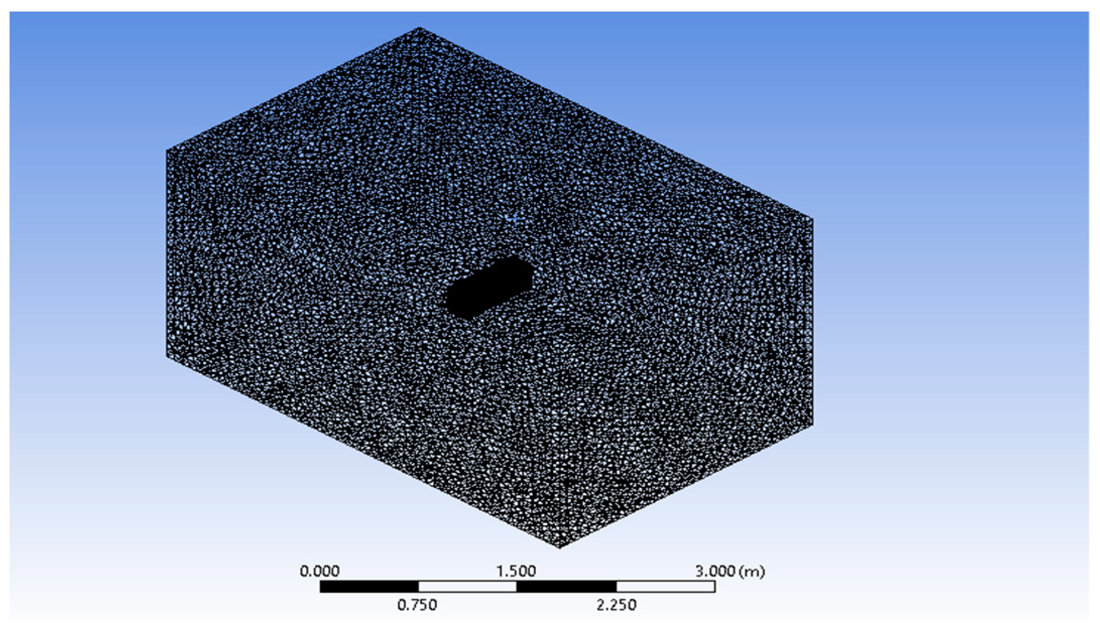
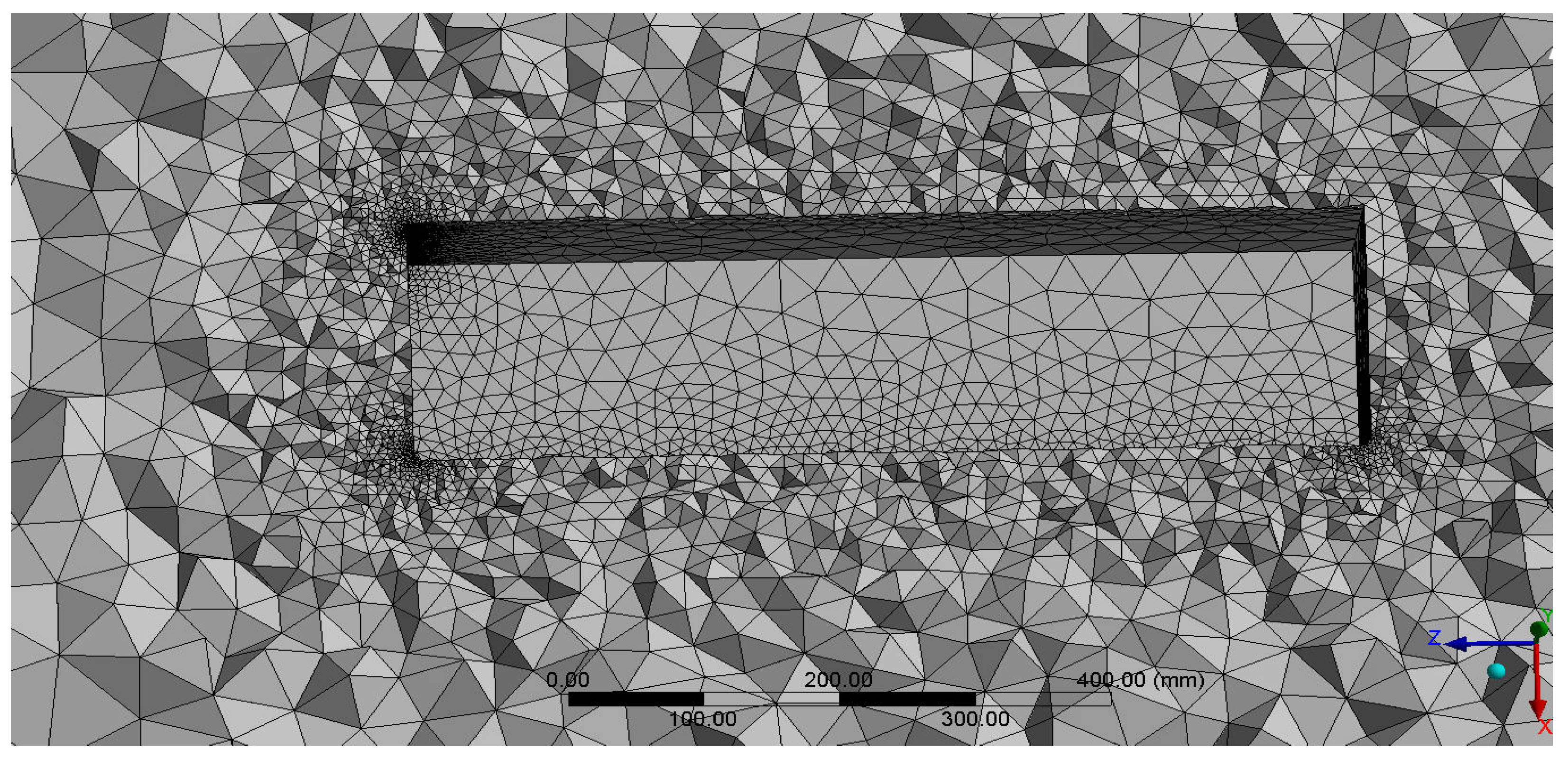
Figure 13.
Wireframe model view of the discretized structure of model IV—area proximity-based unstructured mesh.
Figure 13.
Wireframe model view of the discretized structure of model IV—area proximity-based unstructured mesh.
Figure 14.
Typical view of the fine curvature and proximity with face mesh setup on model VIII.
Figure 14.
Typical view of the fine curvature and proximity with face mesh setup on model VIII.
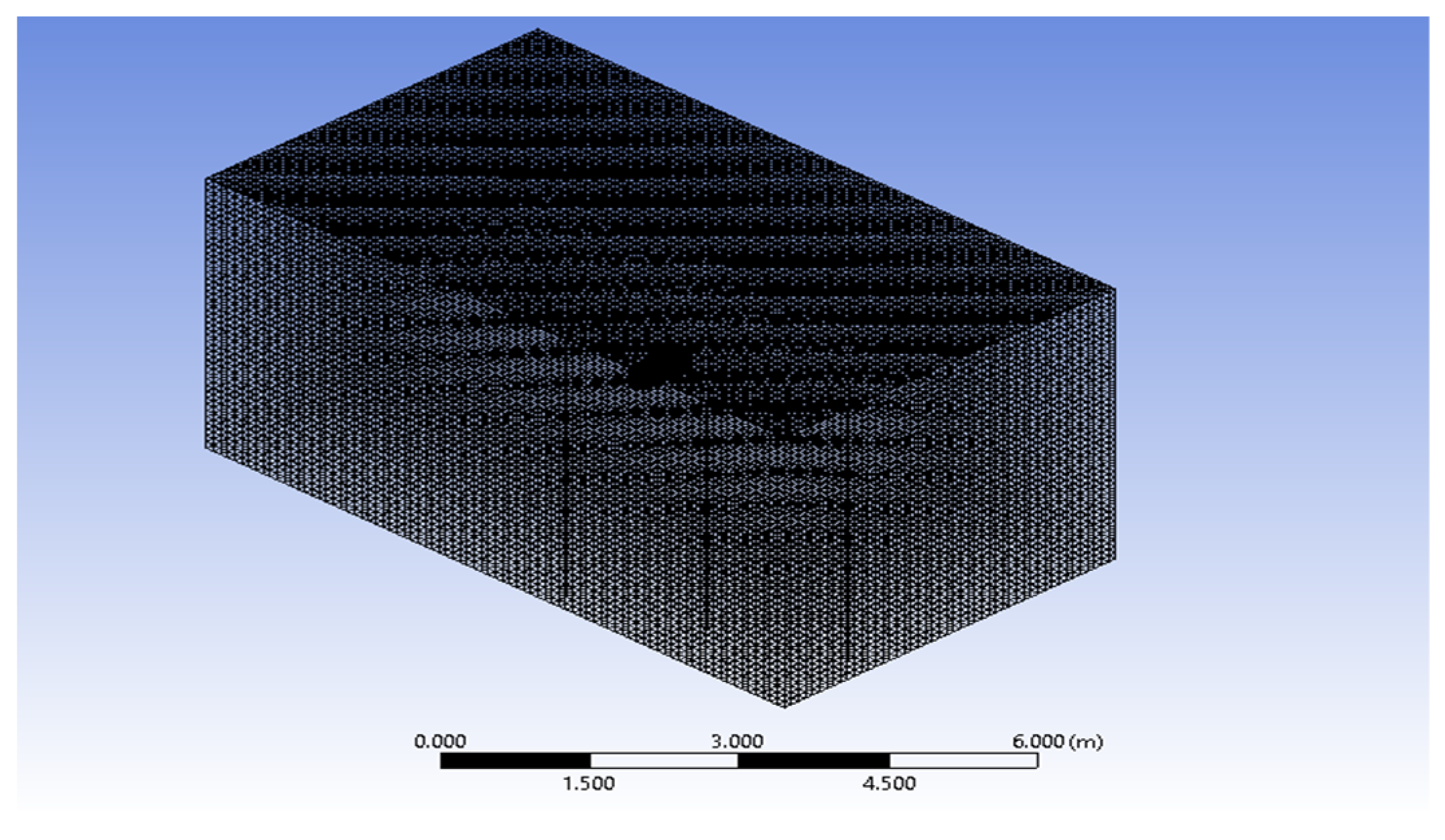
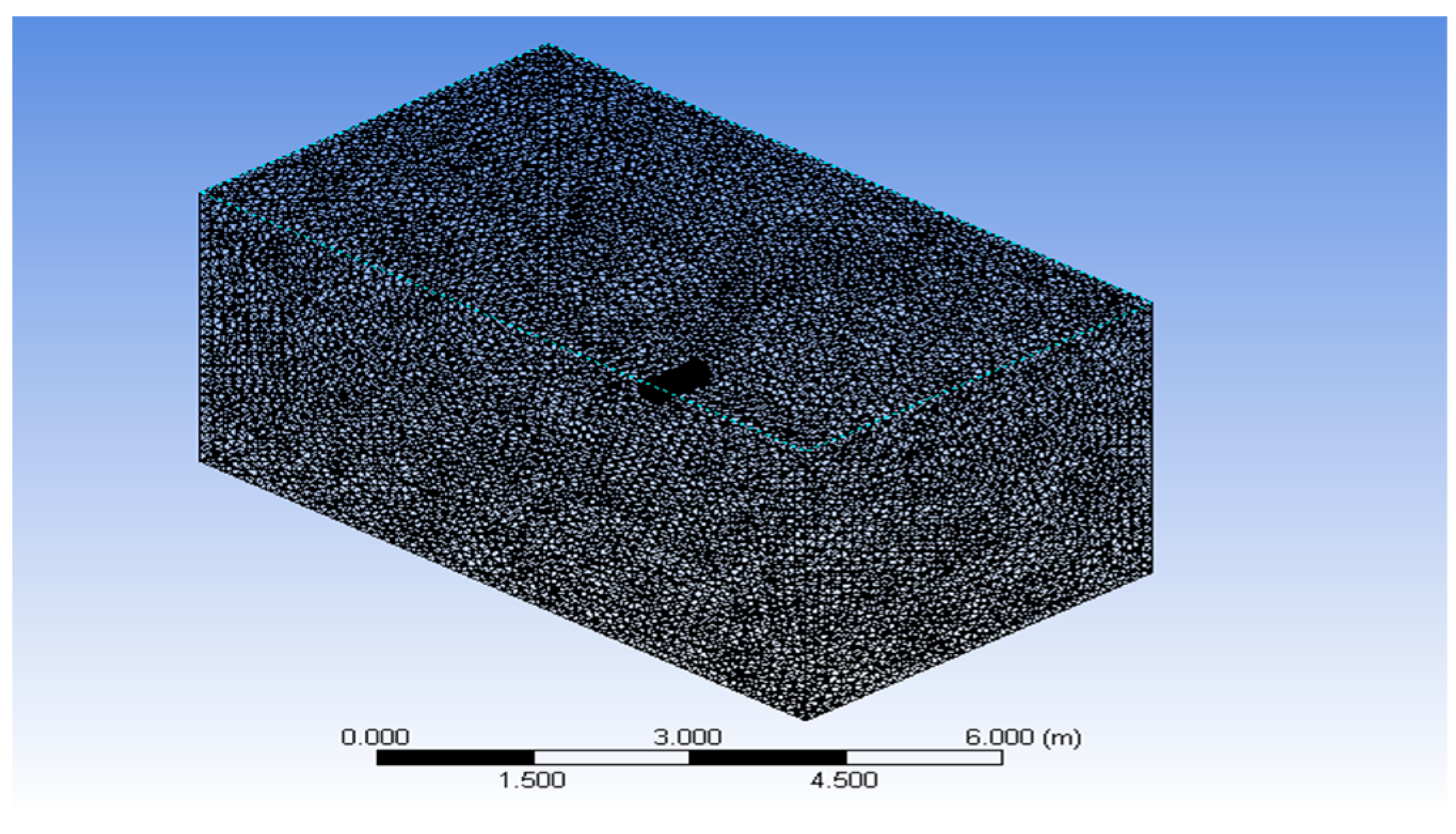
Figure 15.
Typical internal cut-plane view of the entire control volume—sideslip analysis.
Figure 15.
Typical internal cut-plane view of the entire control volume—sideslip analysis.
Figure 16.
Typical internal cut-plane view of the entire control volume—sideslip analysis.
Figure 16.
Typical internal cut-plane view of the entire control volume—sideslip analysis.
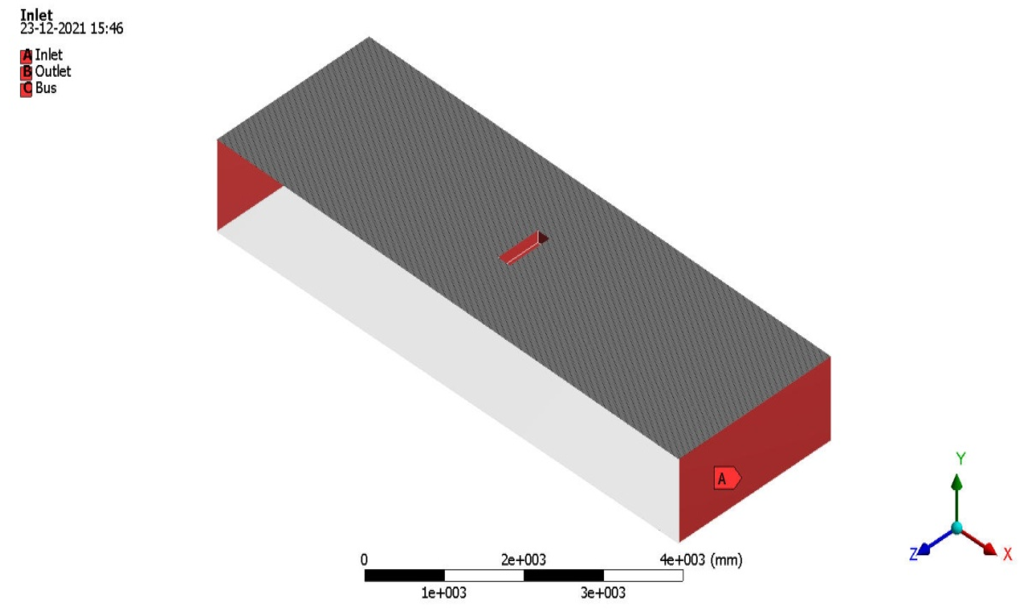
Figure 17.
Details of the initial conditions imposed on the control volume.
Figure 17.
Details of the initial conditions imposed on the control volume.
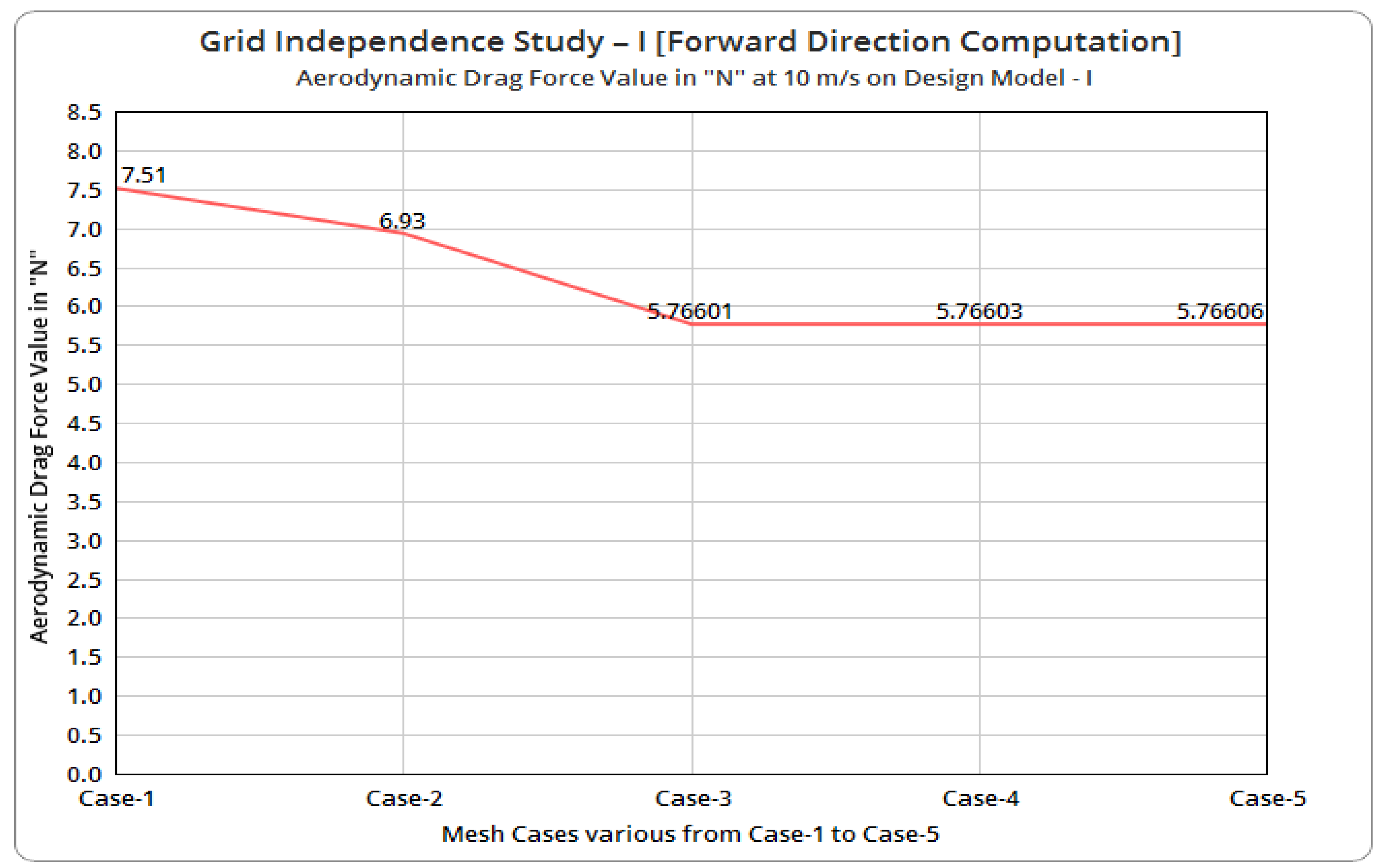
Figure 18.
Comprehensive drag value in N at 10 m/s on model I.
Figure 18.
Comprehensive drag value in N at 10 m/s on model I.
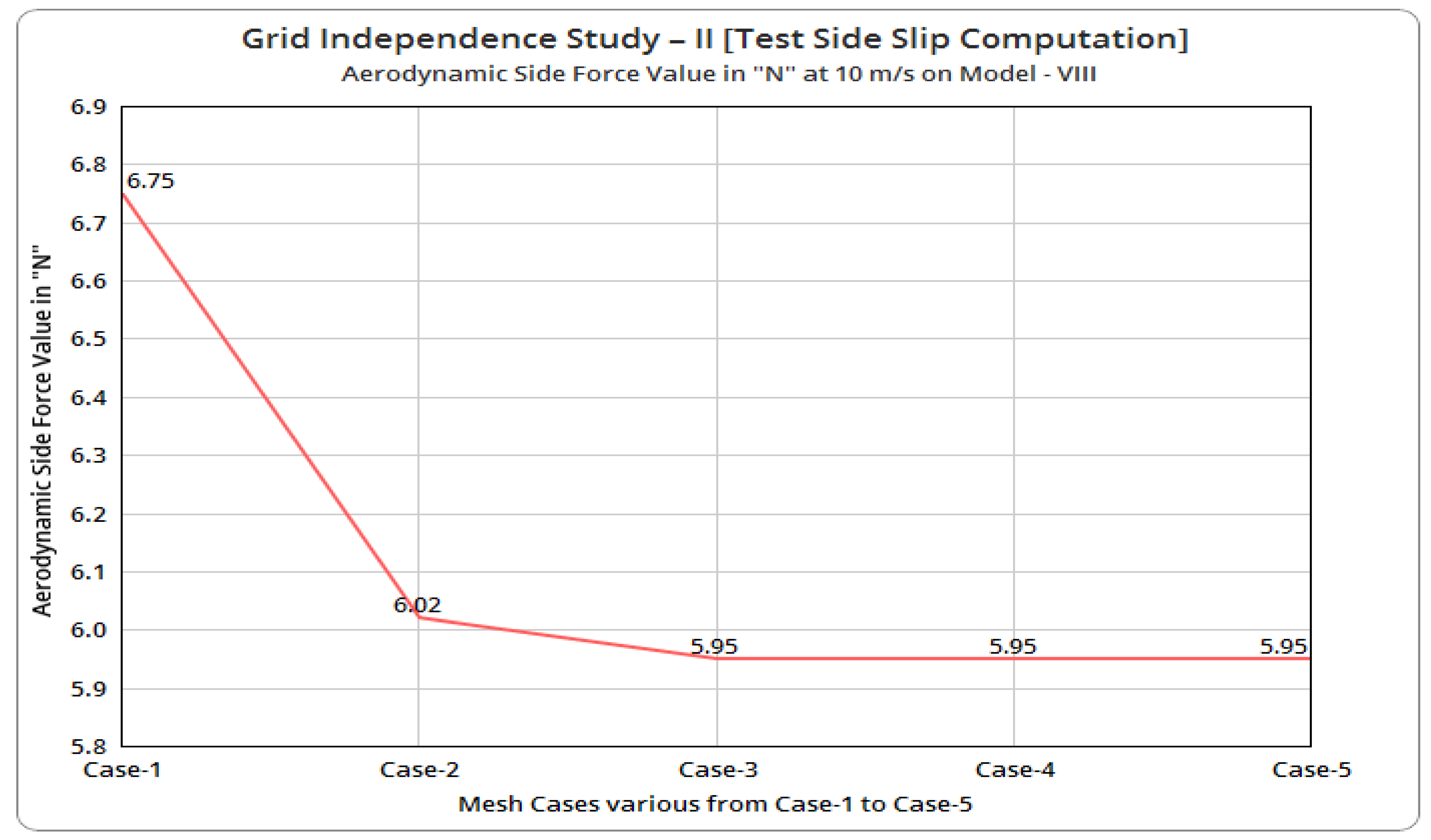
Figure 19.
Comprehensive side force value in N at 10 m/s on model VIII.
Figure 19.
Comprehensive side force value in N at 10 m/s on model VIII.
Figure 20.
Typical full view of the subsonic wind tunnel with the data acquisition system (bottom right).
Figure 20.
Typical full view of the subsonic wind tunnel with the data acquisition system (bottom right).
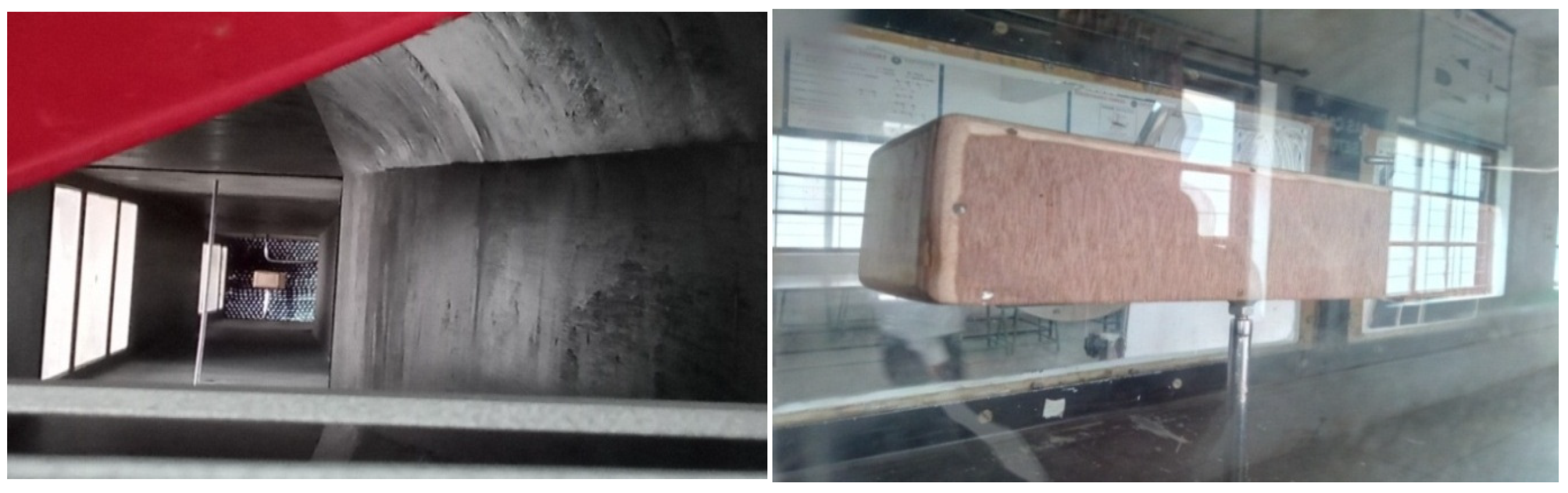
Figure 21.
Typical zoomed-in and normal views of an intercity bus without dimples located in the test section.
Figure 21.
Typical zoomed-in and normal views of an intercity bus without dimples located in the test section.
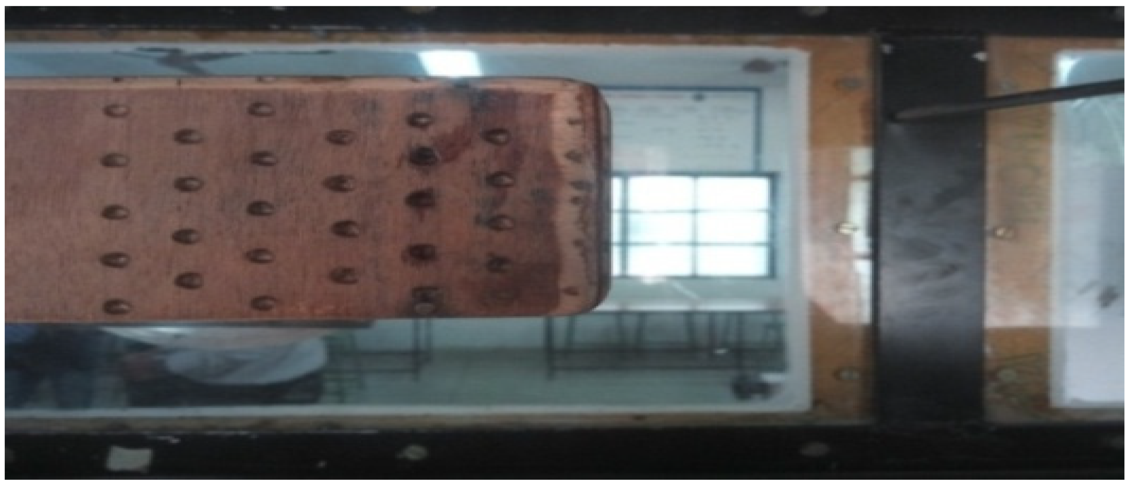
Figure 22.
Typical view of an intercity bus with dimples.
Figure 22.
Typical view of an intercity bus with dimples.
Figure 23.
Velocity distributions over the bus models—tested only for experimental validation.
Figure 23.
Velocity distributions over the bus models—tested only for experimental validation.
Figure 24.
Pressure distributions over the bus models—tested only for experimental validation.
Figure 24.
Pressure distributions over the bus models—tested only for experimental validation.
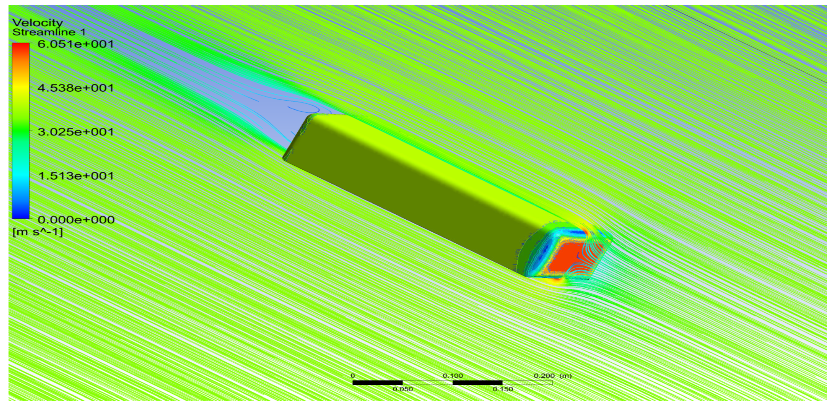
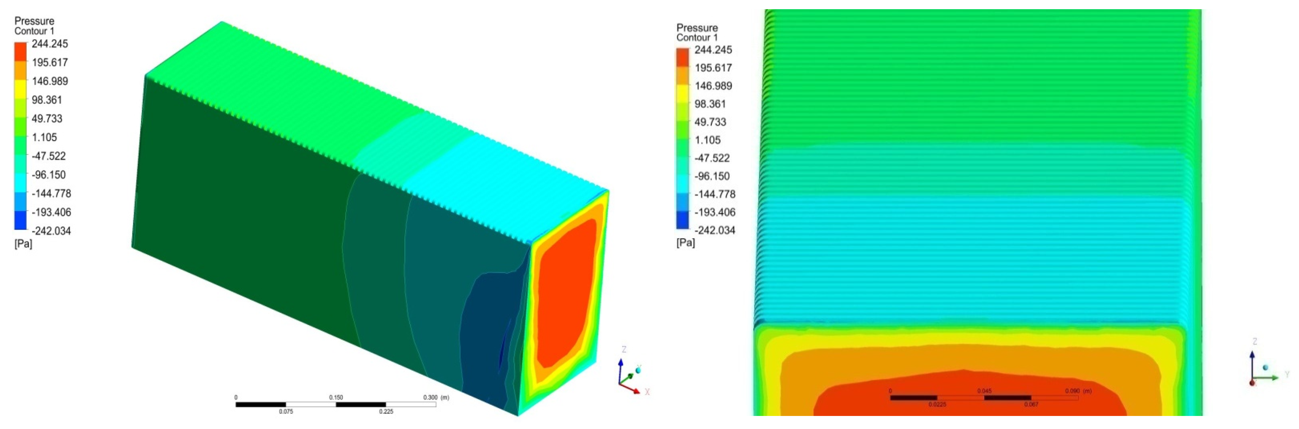
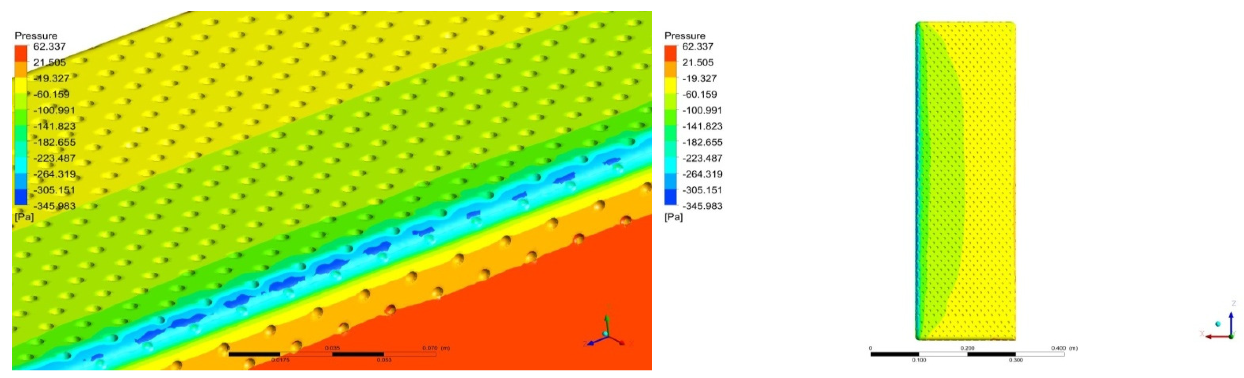
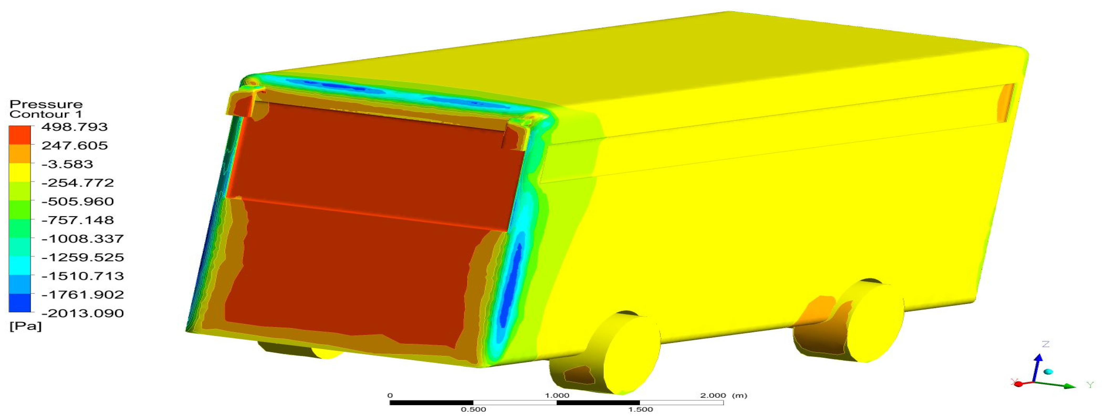
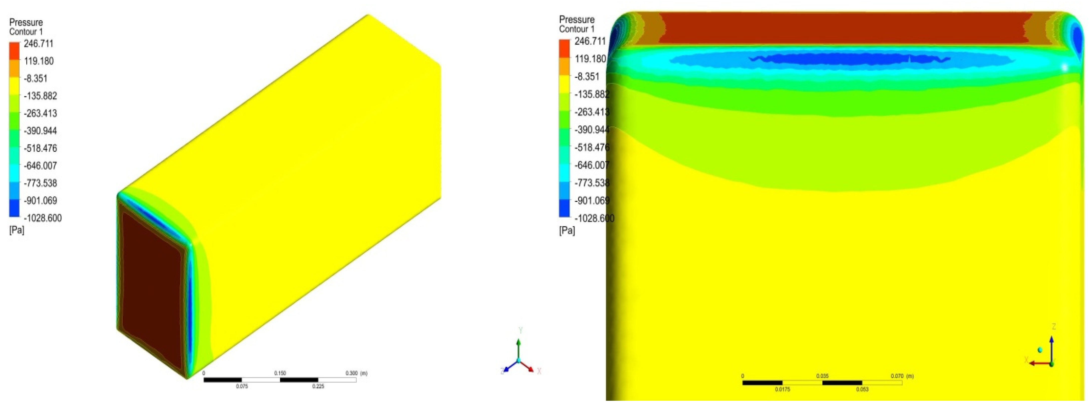
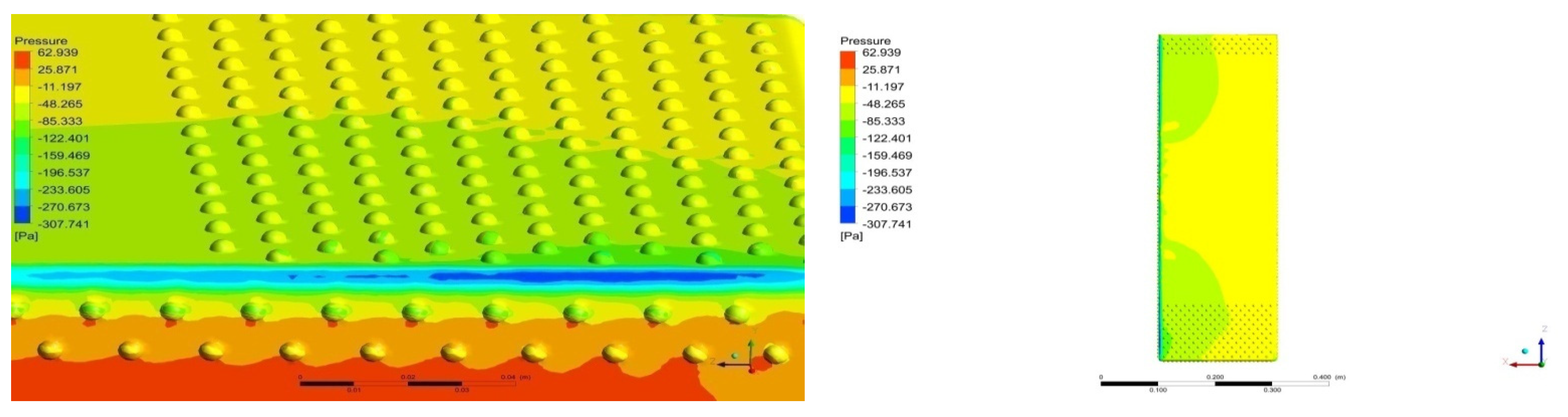
Figure 25.
Typical isometric and zoomed-in frontal views of aerodynamic pressure distributions on the base model.
Figure 25.
Typical isometric and zoomed-in frontal views of aerodynamic pressure distributions on the base model.
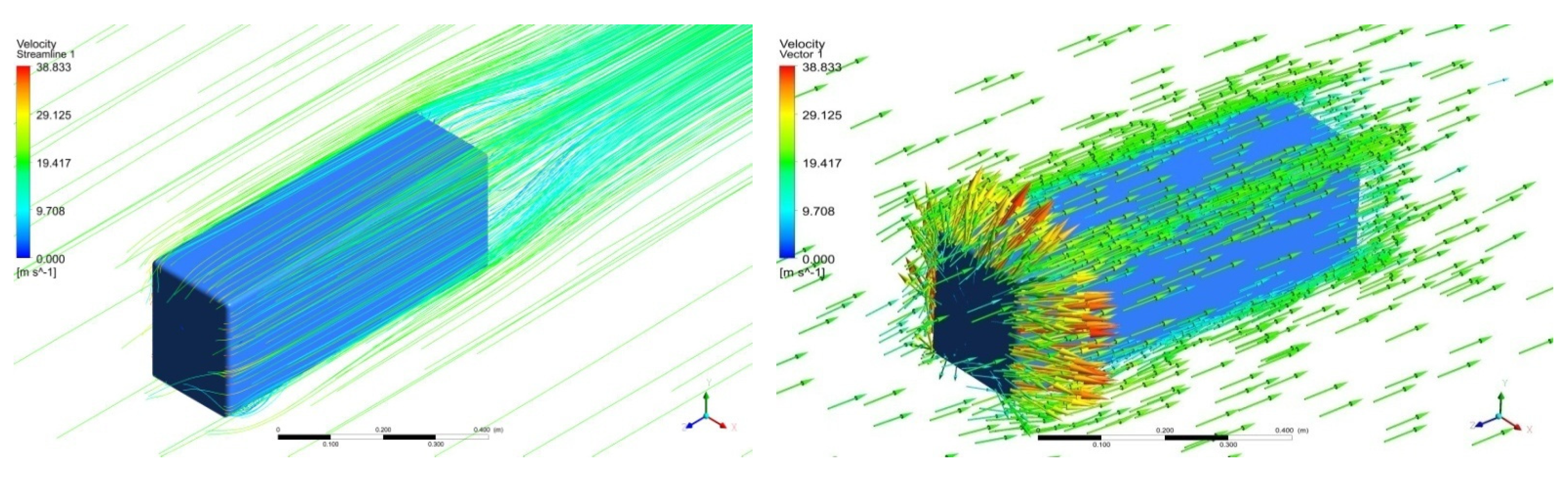
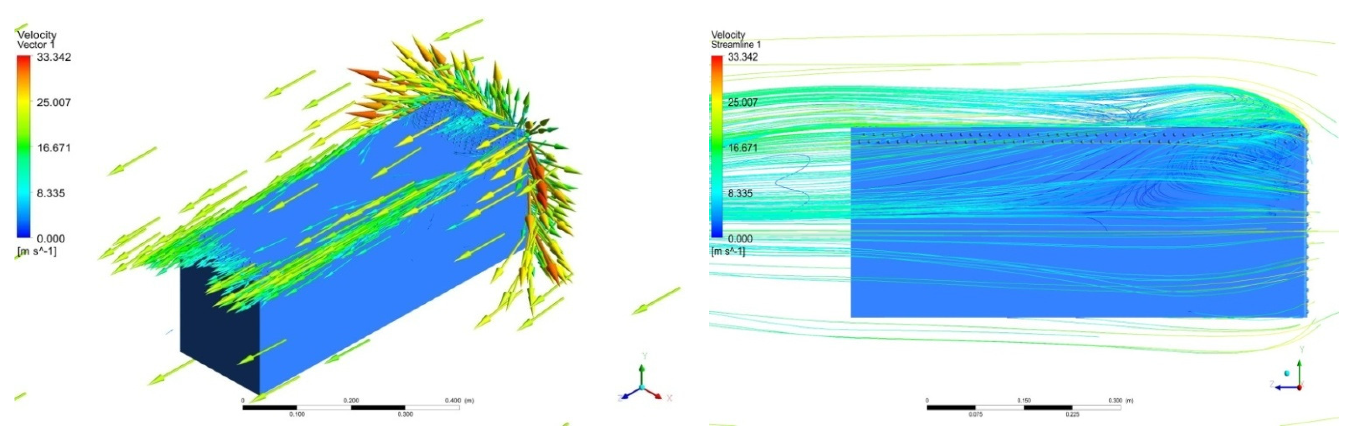
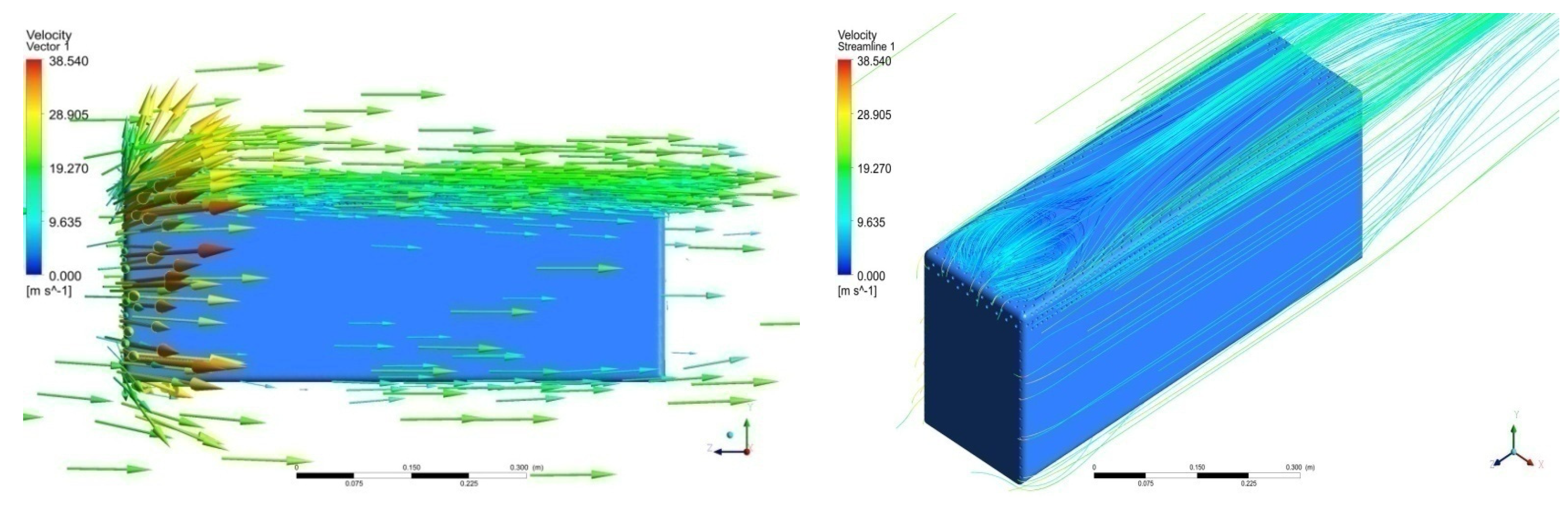
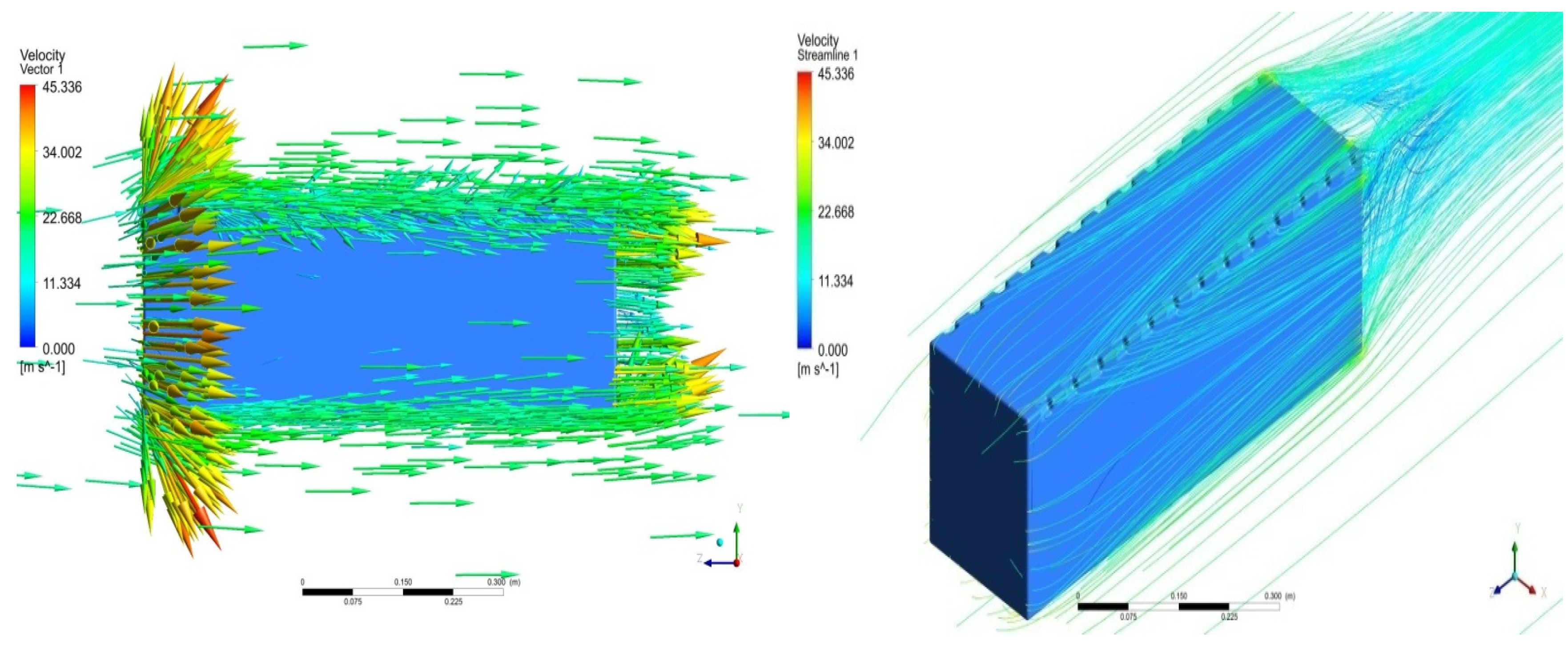
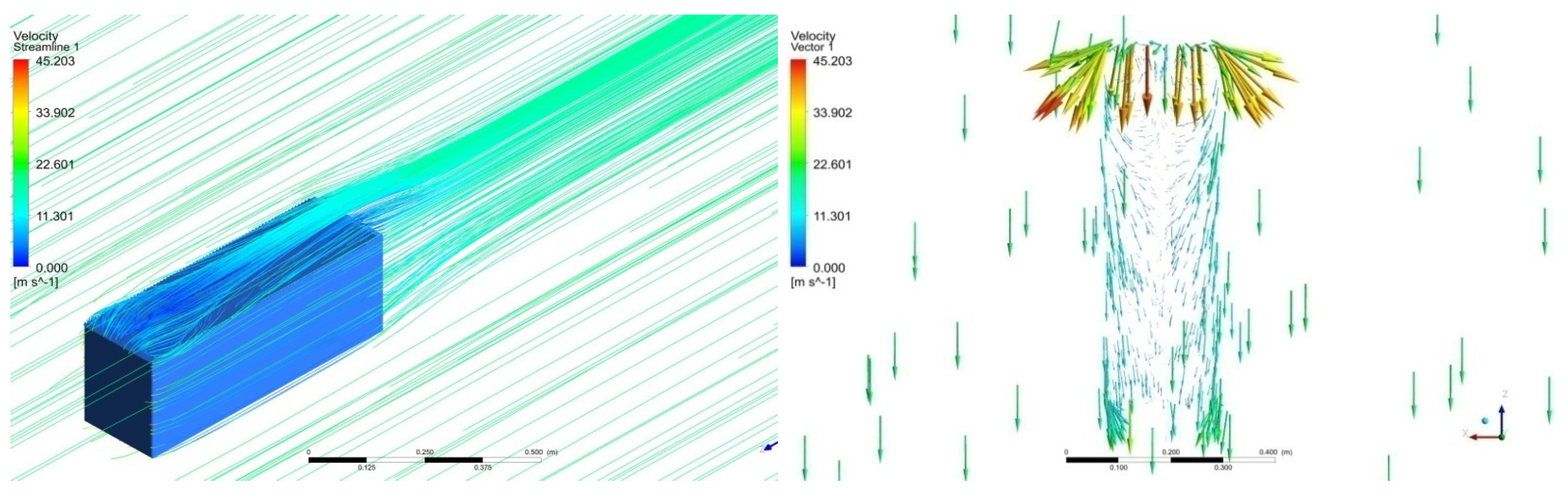
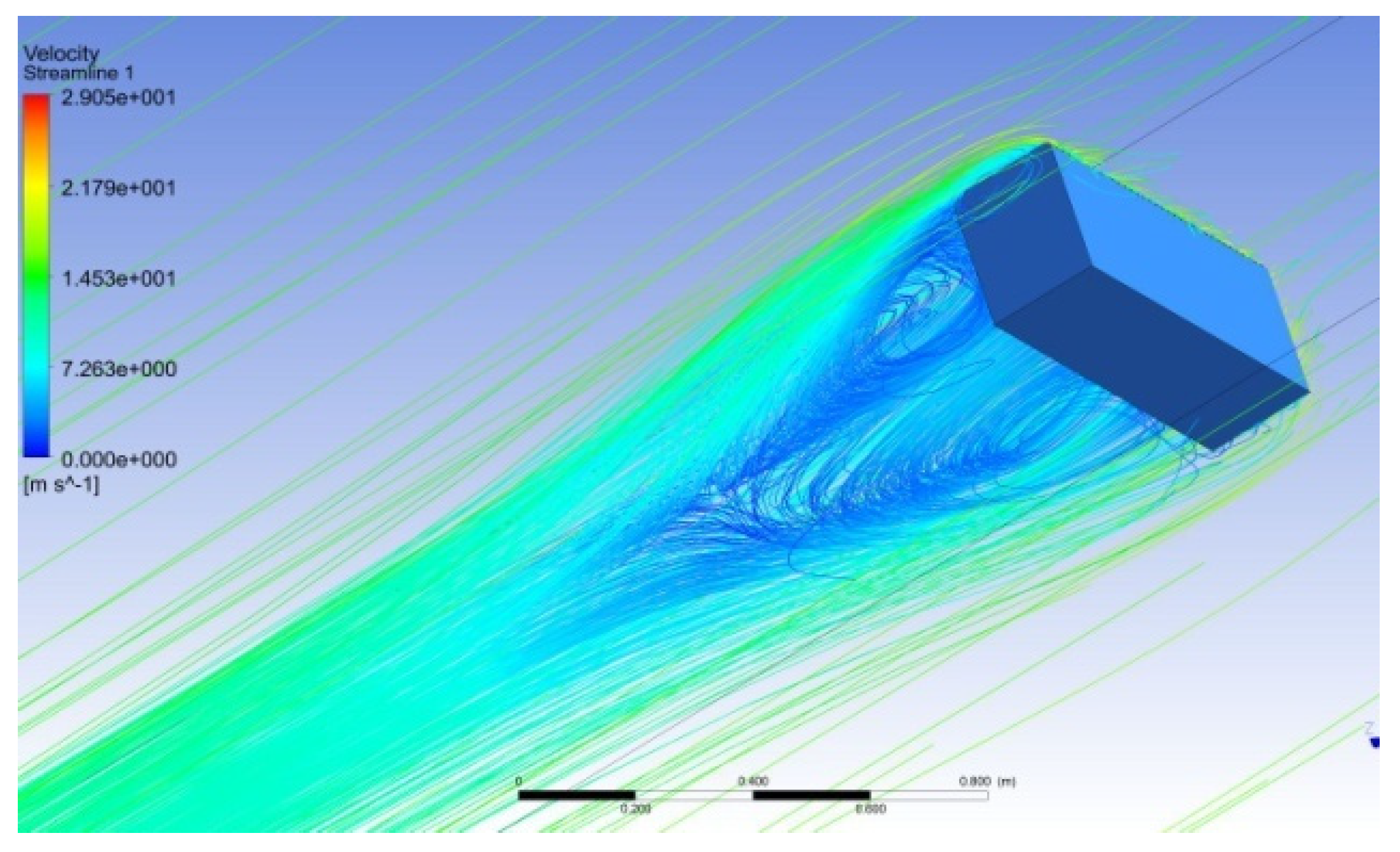
Figure 26.
Streamline- and vector-based representations of air fluid velocity variations over the base model—isometric projections.
Figure 26.
Streamline- and vector-based representations of air fluid velocity variations over the base model—isometric projections.
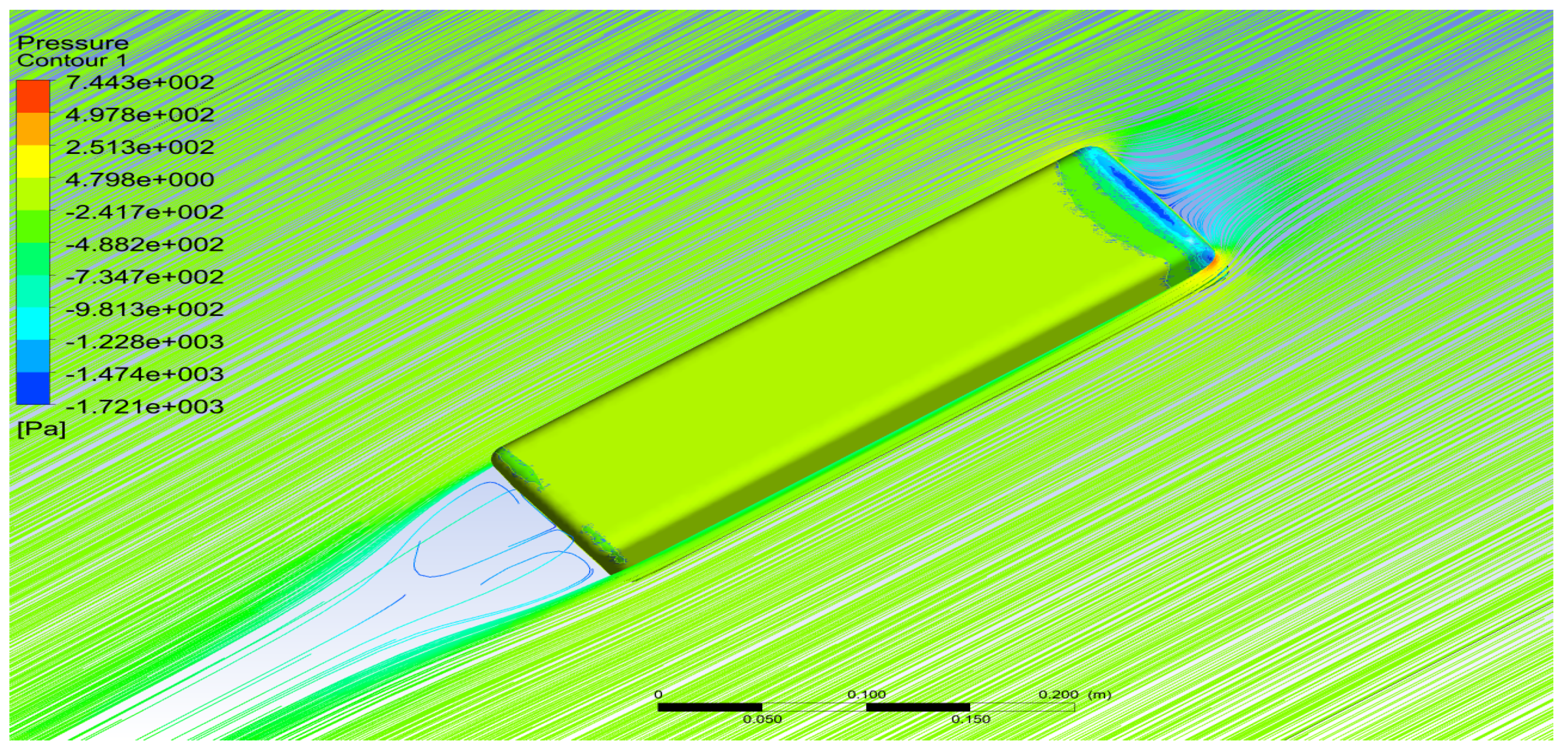
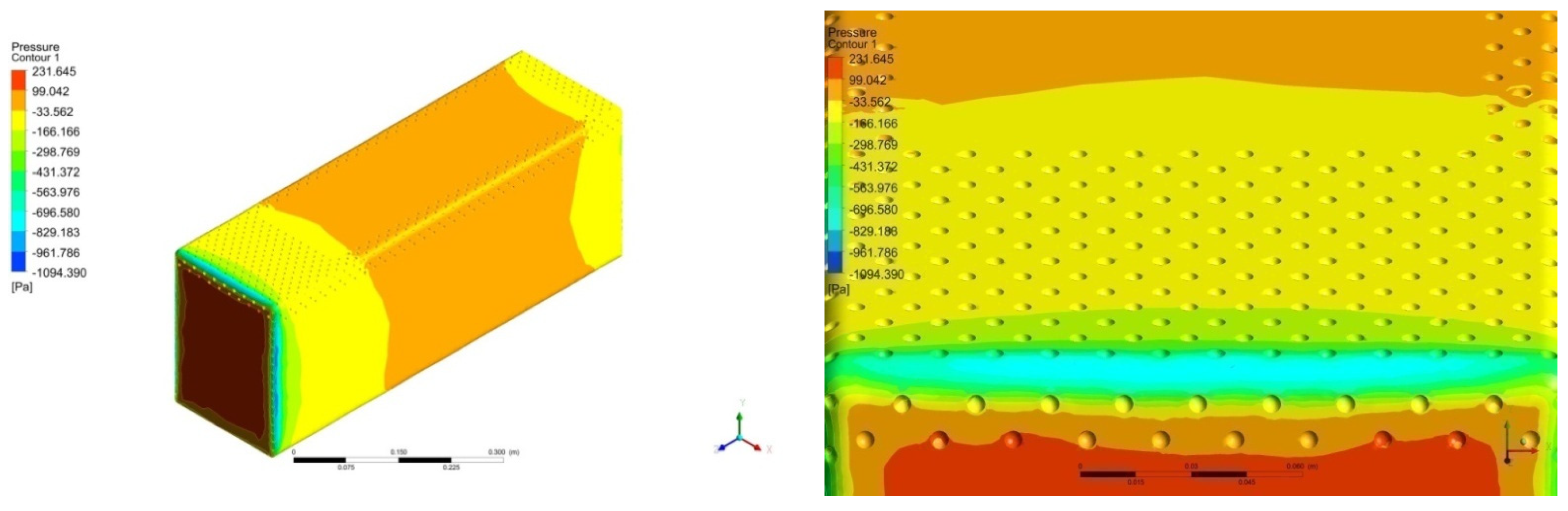
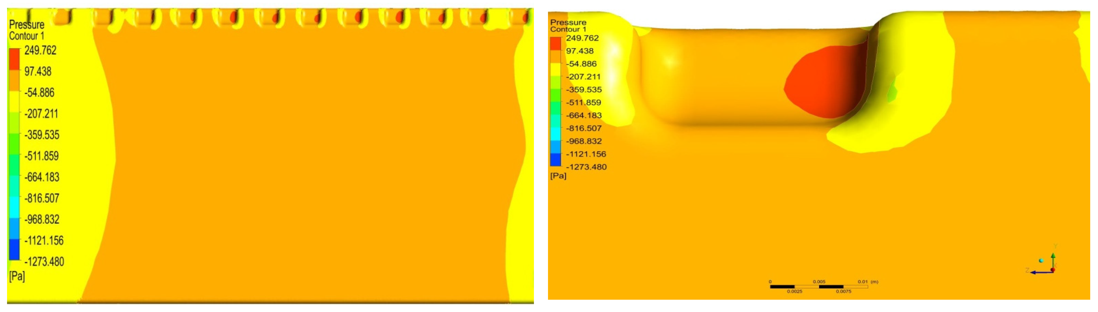
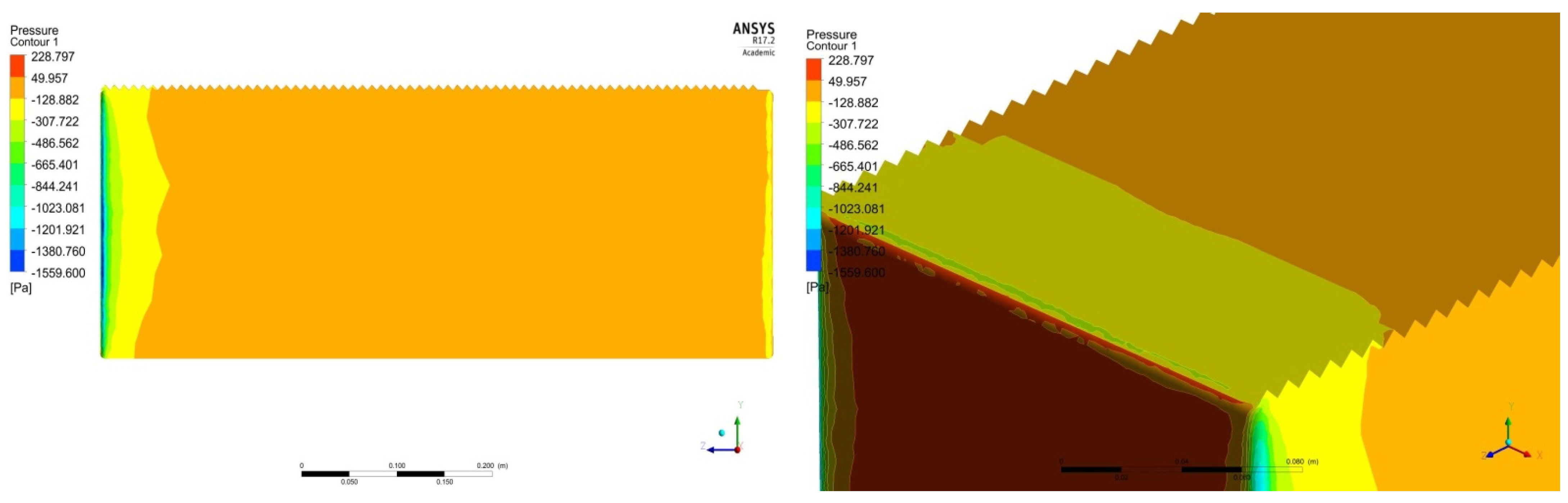
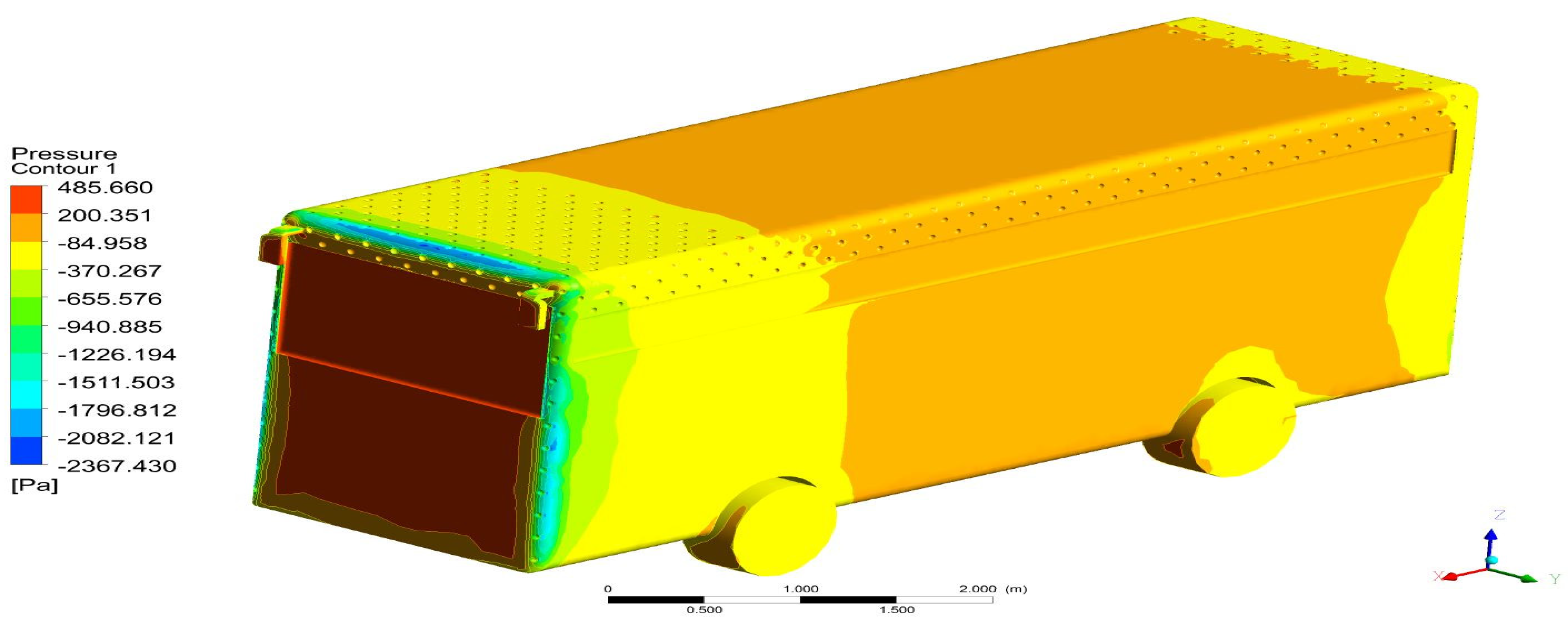
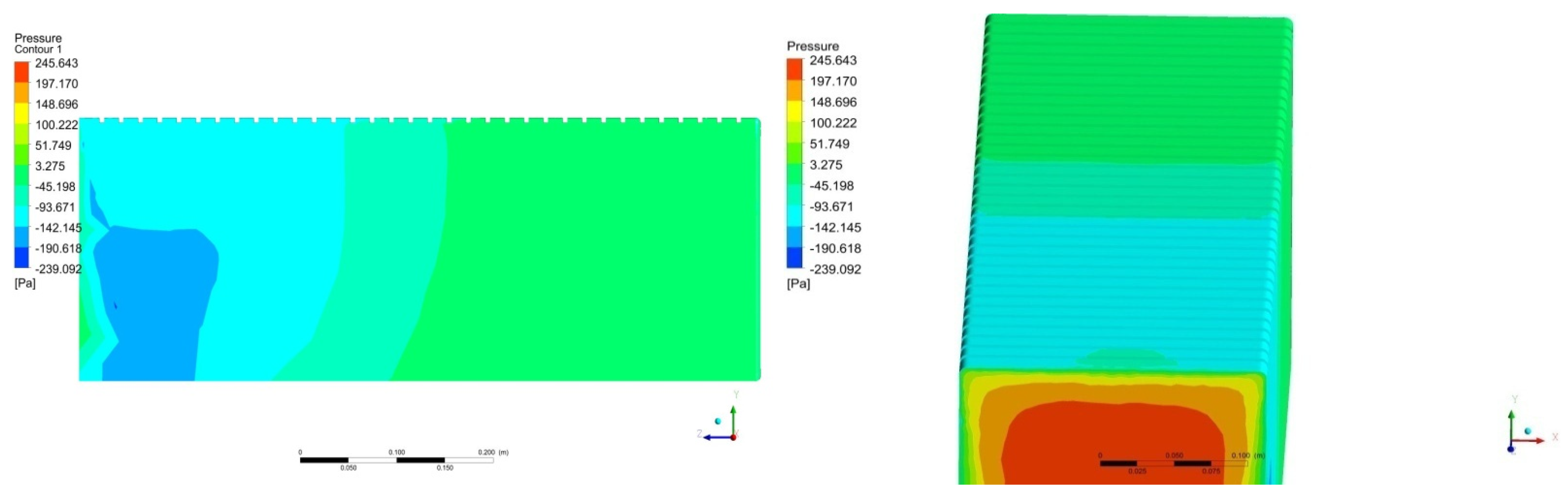
Figure 27.
Methodical side and zoomed-in frontal views of aerodynamic pressure distributions on bus model I.
Figure 27.
Methodical side and zoomed-in frontal views of aerodynamic pressure distributions on bus model I.
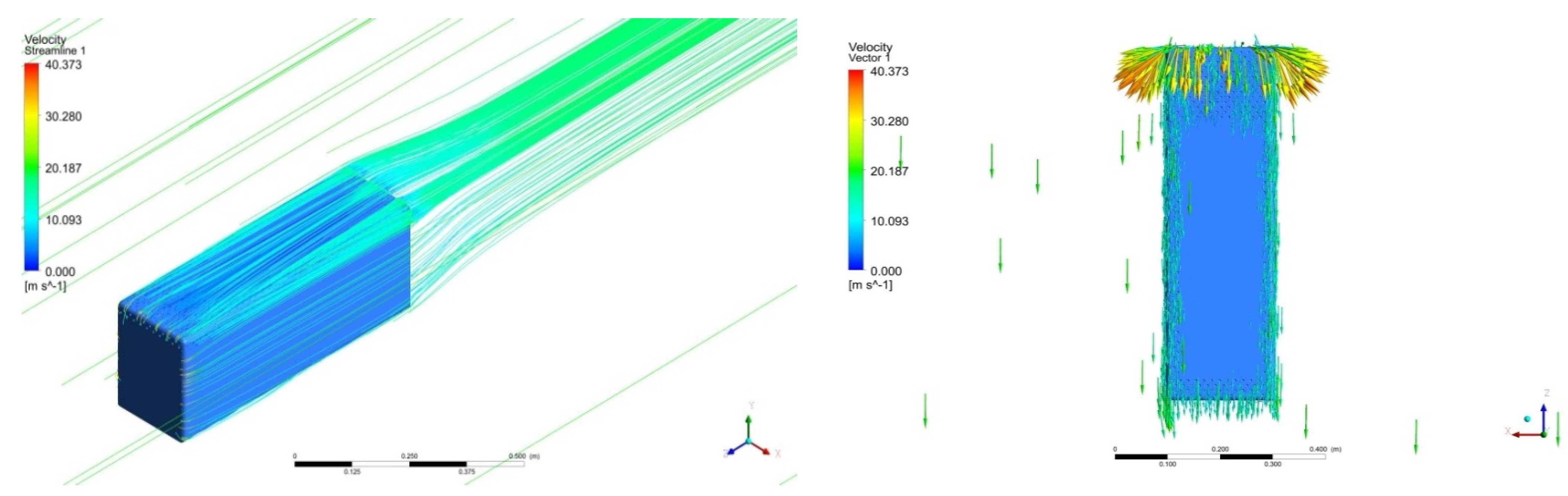
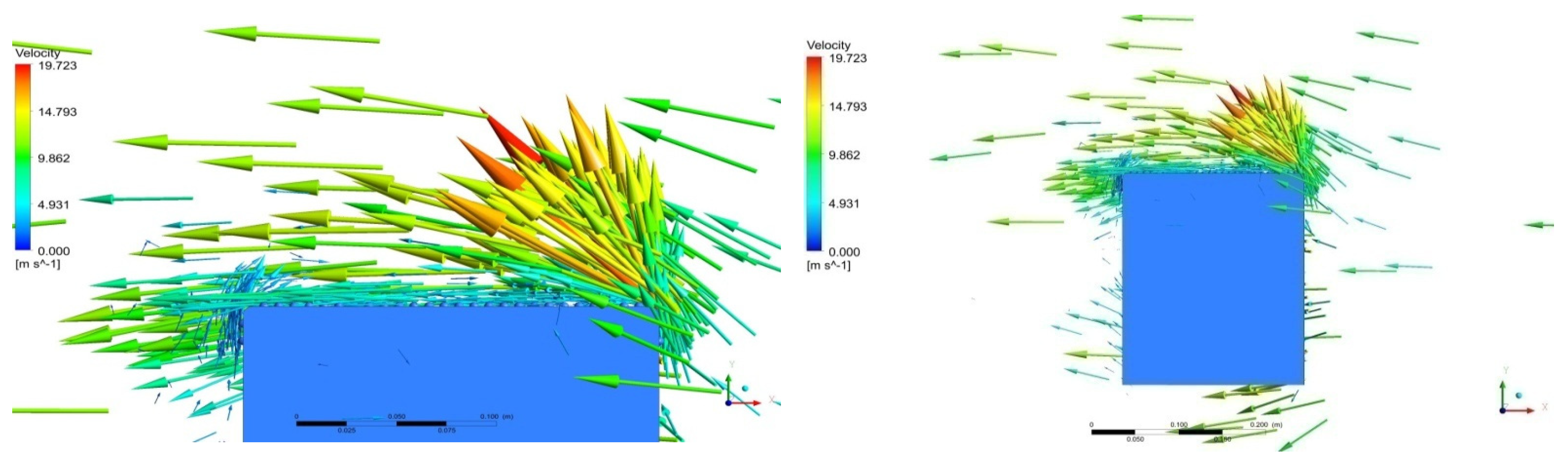
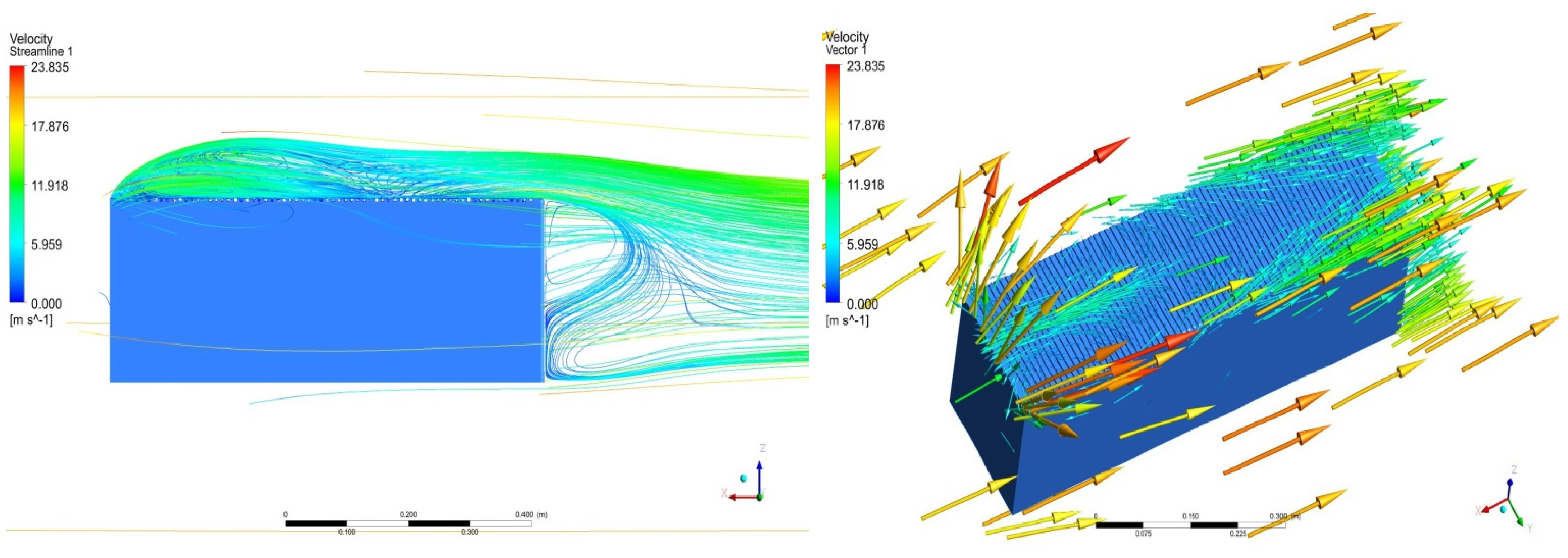
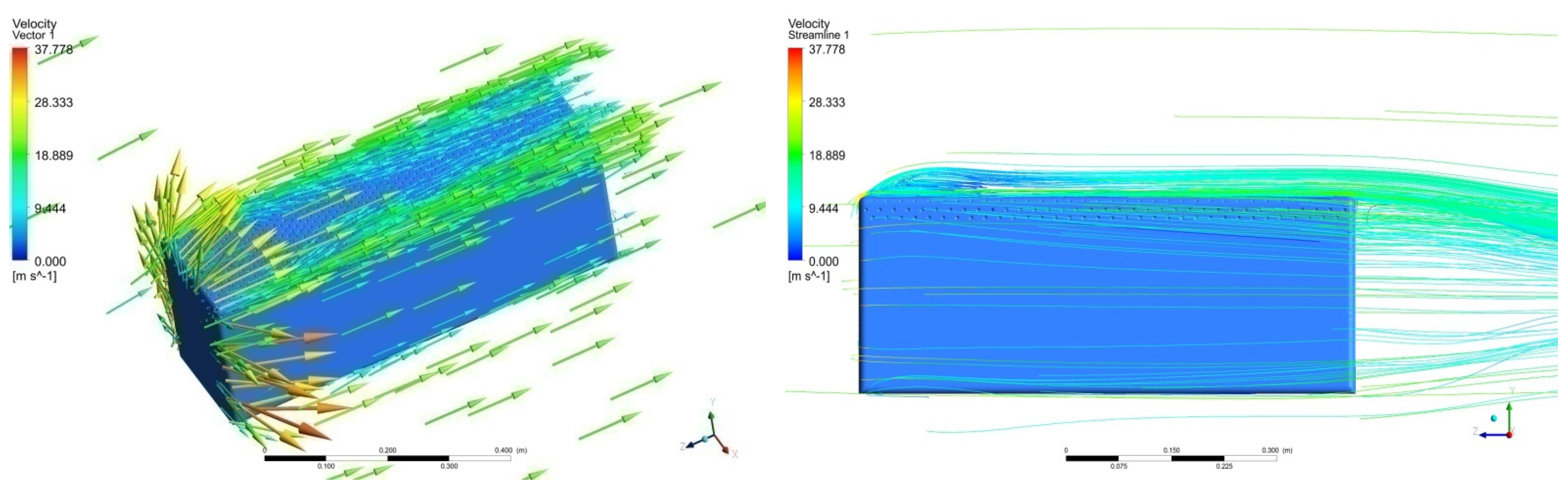
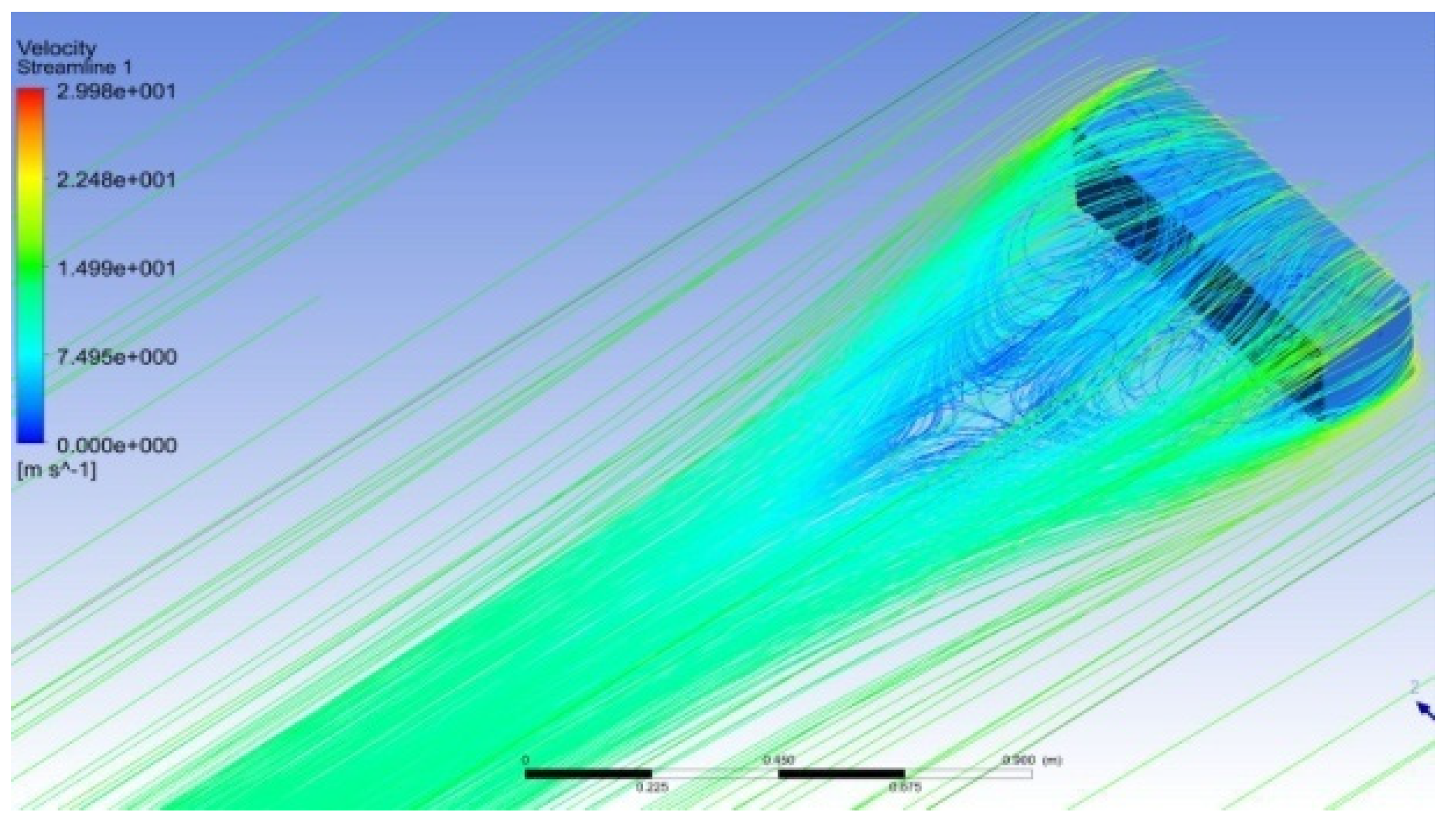
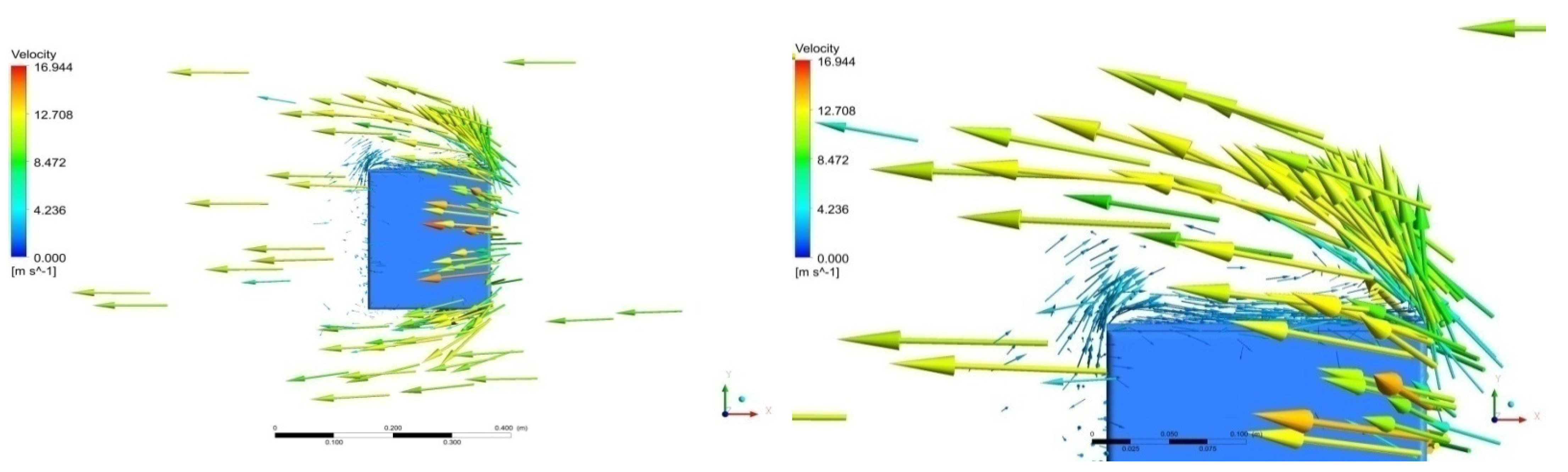
Figure 28.
Vector and streamline-based representations of air fluid velocity variations over the first bus model—side and isometric projections.
Figure 28.
Vector and streamline-based representations of air fluid velocity variations over the first bus model—side and isometric projections.
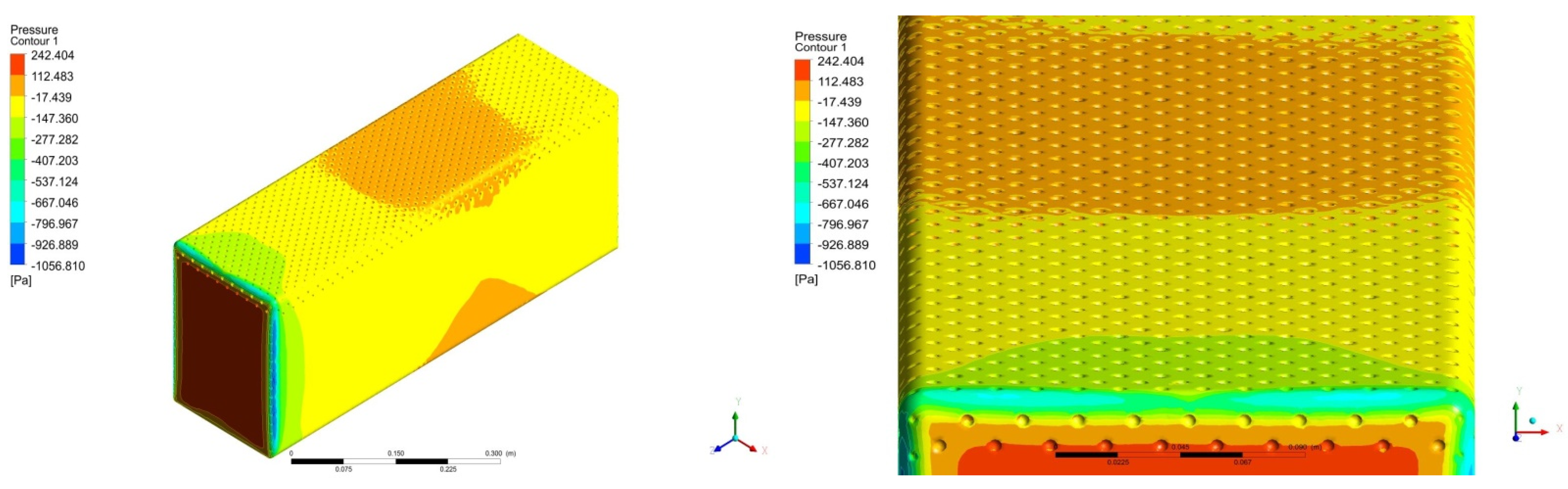
Figure 29.
Systematic representations of isometric and zoomed-in frontal orientations of aerodynamic pressure distributions on the second bus model.
Figure 29.
Systematic representations of isometric and zoomed-in frontal orientations of aerodynamic pressure distributions on the second bus model.
Figure 30.
Streamline- and vector-based representations of air fluid velocity variations over the second bus model—isometric projections.
Figure 30.
Streamline- and vector-based representations of air fluid velocity variations over the second bus model—isometric projections.
Figure 31.
Logical isometric and zoomed-in frontal views of aerodynamic pressure distributions on the third bus model.
Figure 31.
Logical isometric and zoomed-in frontal views of aerodynamic pressure distributions on the third bus model.
Figure 32.
Streamline and vector-based representations of air fluid velocity variations over the third bus model through isometric and top projections.
Figure 32.
Streamline and vector-based representations of air fluid velocity variations over the third bus model through isometric and top projections.
Figure 33.
Emblematic side and zoomed-in frontal views of aerodynamic pressure distributions on the fourth bus model.
Figure 33.
Emblematic side and zoomed-in frontal views of aerodynamic pressure distributions on the fourth bus model.
Figure 34.
Vector- and streamline-based representations of air fluid velocity variations over the fourth bus model with the help of top and isometric projections.
Figure 34.
Vector- and streamline-based representations of air fluid velocity variations over the fourth bus model with the help of top and isometric projections.
Figure 35.
Organized isometric and zoomed-in frontal views of aerodynamic pressure distributions on the fifth bus model.
Figure 35.
Organized isometric and zoomed-in frontal views of aerodynamic pressure distributions on the fifth bus model.
Figure 36.
Streamline- and vector-based representations of air fluid velocity variations over the fifth bus model through side and isometric projections.
Figure 36.
Streamline- and vector-based representations of air fluid velocity variations over the fifth bus model through side and isometric projections.
Figure 37.
Classic side and zoomed-in lengthwise positioned views of aerodynamic pressure distributions on the sixth bus model.
Figure 37.
Classic side and zoomed-in lengthwise positioned views of aerodynamic pressure distributions on the sixth bus model.
Figure 38.
Streamline- and vector-based representations of air fluid velocity variations on the sixth bus model through isometric and top projections.
Figure 38.
Streamline- and vector-based representations of air fluid velocity variations on the sixth bus model through isometric and top projections.
Figure 39.
Typical side and zoomed-in isometric views of aerodynamic pressure distributions on the seventh bus model.
Figure 39.
Typical side and zoomed-in isometric views of aerodynamic pressure distributions on the seventh bus model.
Figure 40.
Streamline- and vector-based representations of air fluid velocity variations on the seventh bus model—isometric- and top-oriented projections.
Figure 40.
Streamline- and vector-based representations of air fluid velocity variations on the seventh bus model—isometric- and top-oriented projections.
Figure 41.
Characteristic views of aerodynamic pressure distributions on the eighth bus model using isometric and top-oriented projections.
Figure 41.
Characteristic views of aerodynamic pressure distributions on the eighth bus model using isometric and top-oriented projections.
Figure 42.
Vector and streamline-based representations of air fluid velocity variations on the eighth bus model.
Figure 42.
Vector and streamline-based representations of air fluid velocity variations on the eighth bus model.
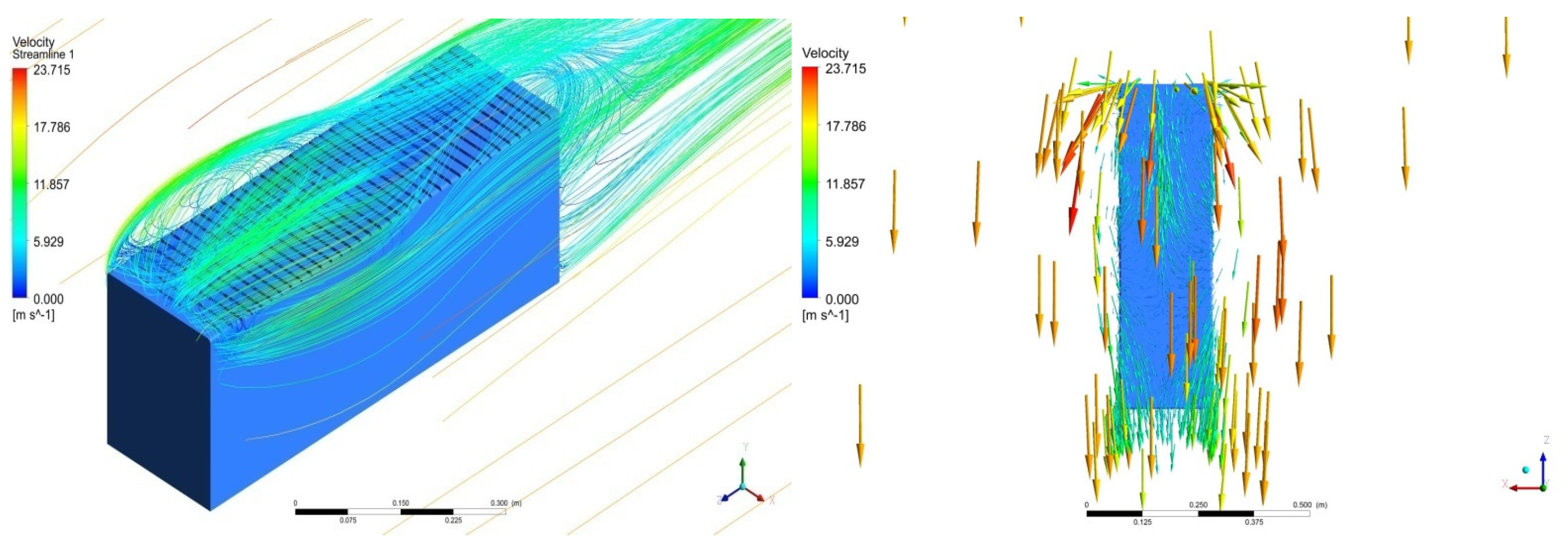
Figure 43.
Representations of sideslip flow velocity distributions over the first bus model.
Figure 43.
Representations of sideslip flow velocity distributions over the first bus model.
Figure 44.
Representations of the dynamic pressure decrement in the presence of dimples in the first model.
Figure 44.
Representations of the dynamic pressure decrement in the presence of dimples in the first model.
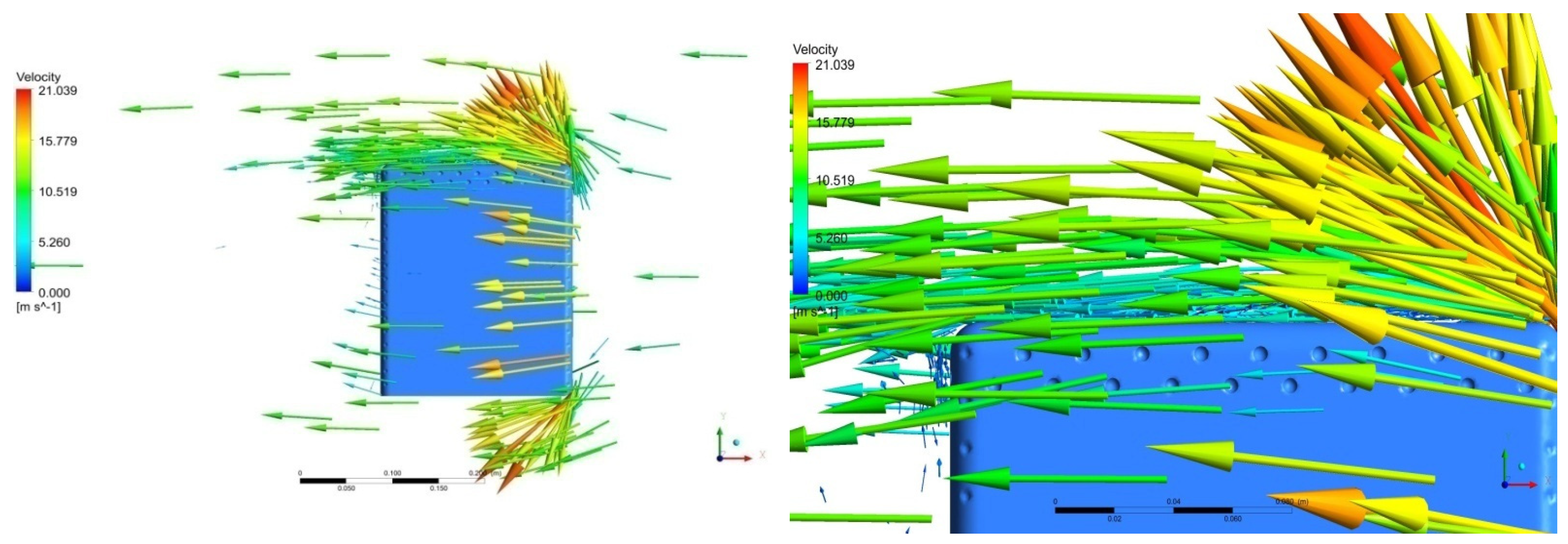
Figure 45.
Systematic views of velocity distributions over the second bus model.
Figure 45.
Systematic views of velocity distributions over the second bus model.
Figure 46.
Archetypal views of dynamic pressure variations over the inverted dimples loaded on the bus surfaces.
Figure 46.
Archetypal views of dynamic pressure variations over the inverted dimples loaded on the bus surfaces.
Figure 47.
A typical isometric view of pressure variations on the third bus model.
Figure 47.
A typical isometric view of pressure variations on the third bus model.
Figure 48.
Streamline-based isometric representation of velocity distributions over the third bus model.
Figure 48.
Streamline-based isometric representation of velocity distributions over the third bus model.
Figure 49.
Typical isometric view of pressure variations on model IV.
Figure 49.
Typical isometric view of pressure variations on model IV.
Figure 50.
Typical representation of velocity distributions over model IV.
Figure 50.
Typical representation of velocity distributions over model IV.
Figure 51.
Typical isometric view of pressure variations on model V.
Figure 51.
Typical isometric view of pressure variations on model V.
Figure 52.
Typical representation of velocity distributions over model V.
Figure 52.
Typical representation of velocity distributions over model V.
Figure 53.
Typical isometric view of pressure variations on model VI.
Figure 53.
Typical isometric view of pressure variations on model VI.
Figure 54.
Typical representation of velocity distributions over model VI.
Figure 54.
Typical representation of velocity distributions over model VI.
Figure 55.
Systematic views of velocity distributions over bus model VII.
Figure 55.
Systematic views of velocity distributions over bus model VII.
Figure 56.
Representative views of dynamic pressure variations over the fins loaded on the bus surfaces.
Figure 56.
Representative views of dynamic pressure variations over the fins loaded on the bus surfaces.
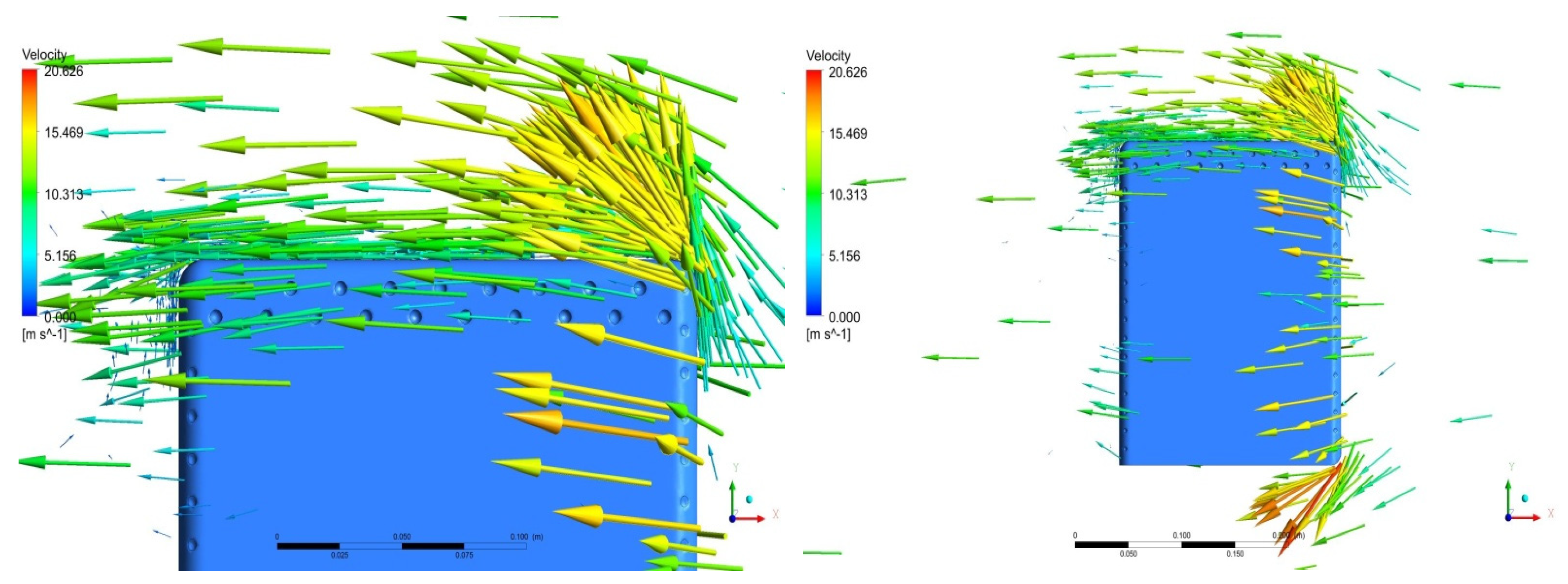
Figure 57.
Systematic views of velocity distributions over bus model VIII.
Figure 57.
Systematic views of velocity distributions over bus model VIII.
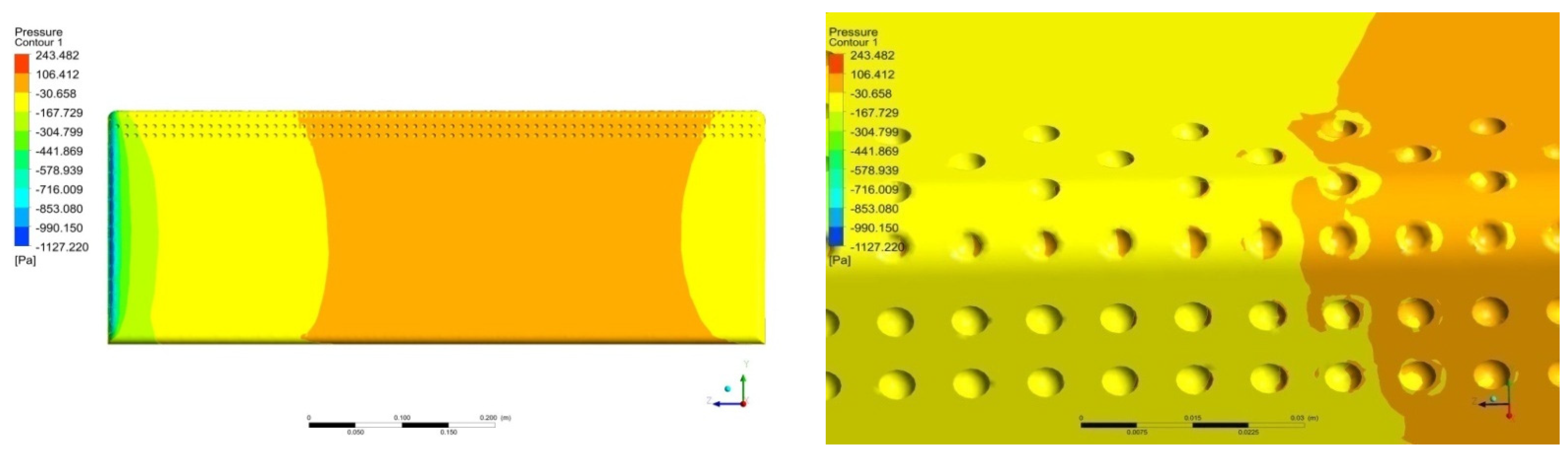
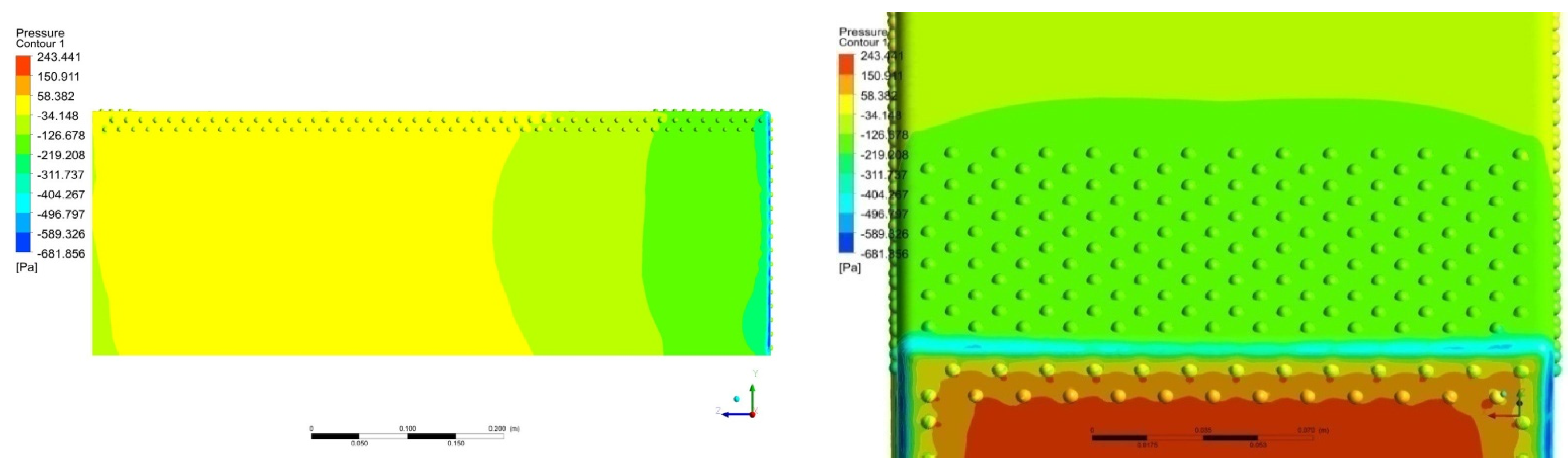
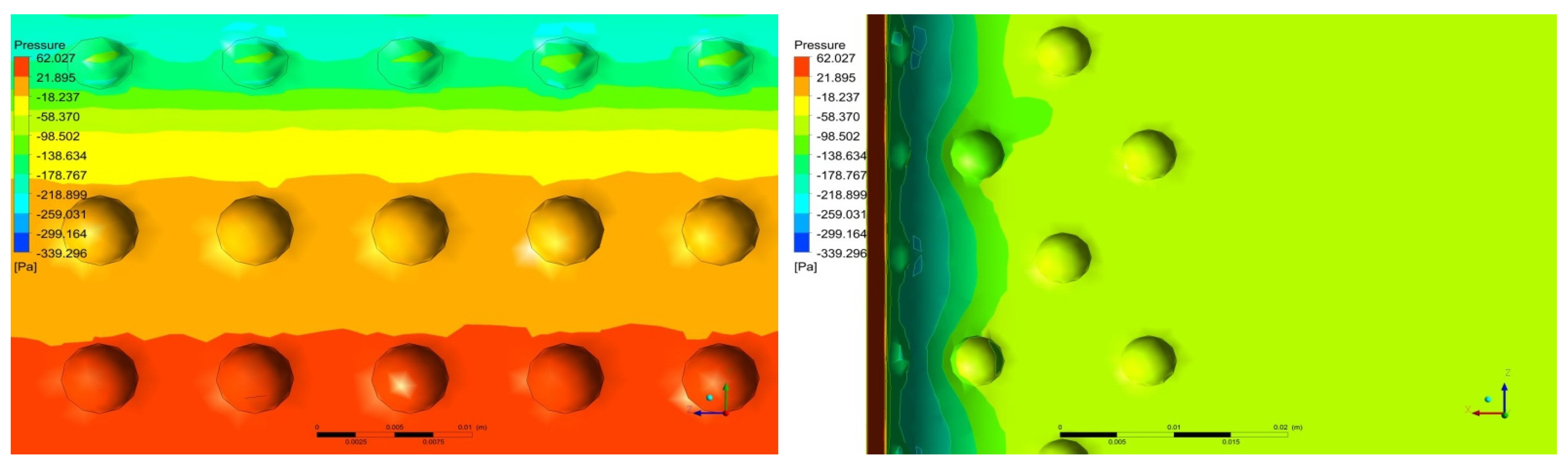
Figure 58.
Exemplary views of dynamic pressure variations over the dimples loaded on the bus surfaces.
Figure 58.
Exemplary views of dynamic pressure variations over the dimples loaded on the bus surfaces.
Figure 59.
Systematic top view-based representation of an intercity bus without dimples (base model).
Figure 59.
Systematic top view-based representation of an intercity bus without dimples (base model).
Figure 60.
Typical side view of an intercity bus loaded with 30 mm dimples in the optimized regions.
Figure 60.
Typical side view of an intercity bus loaded with 30 mm dimples in the optimized regions.
Figure 61.
Typical isometric representation of a bus equipped with 50 mm dimples in the optimized regions.
Figure 61.
Typical isometric representation of a bus equipped with 50 mm dimples in the optimized regions.
Figure 62.
Typical isometric representation of a bus equipped with 75 mm dimples in the optimized regions.
Figure 62.
Typical isometric representation of a bus equipped with 75 mm dimples in the optimized regions.
Figure 63.
Typical isometric representation of a bus equipped with 100 mm dimples in the optimized regions.
Figure 63.
Typical isometric representation of a bus equipped with 100 mm dimples in the optimized regions.
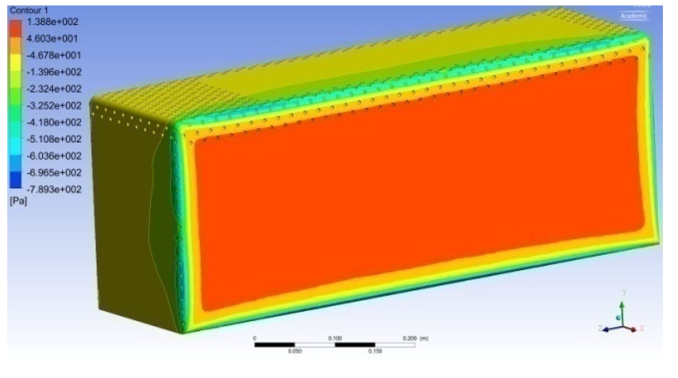
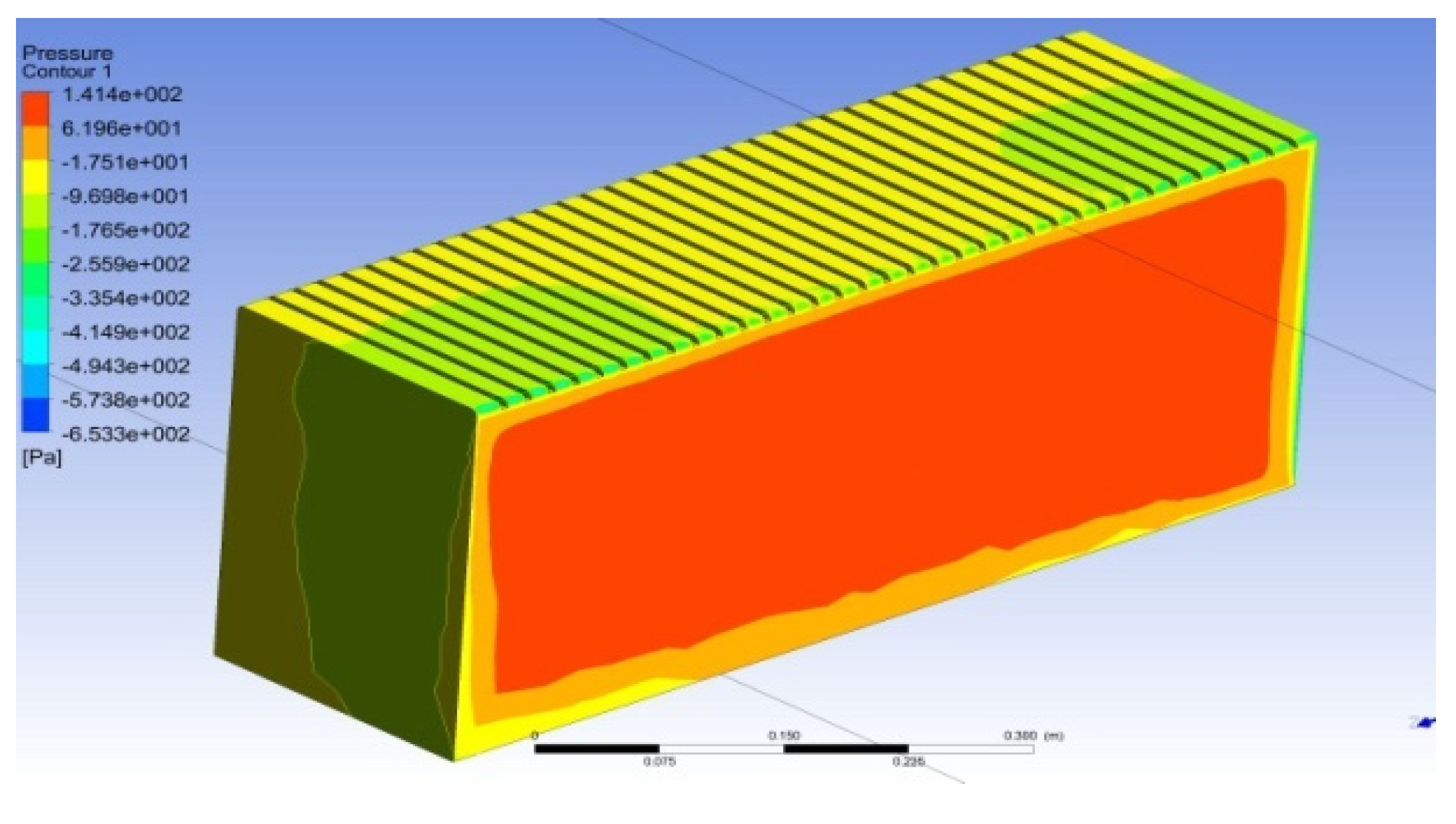
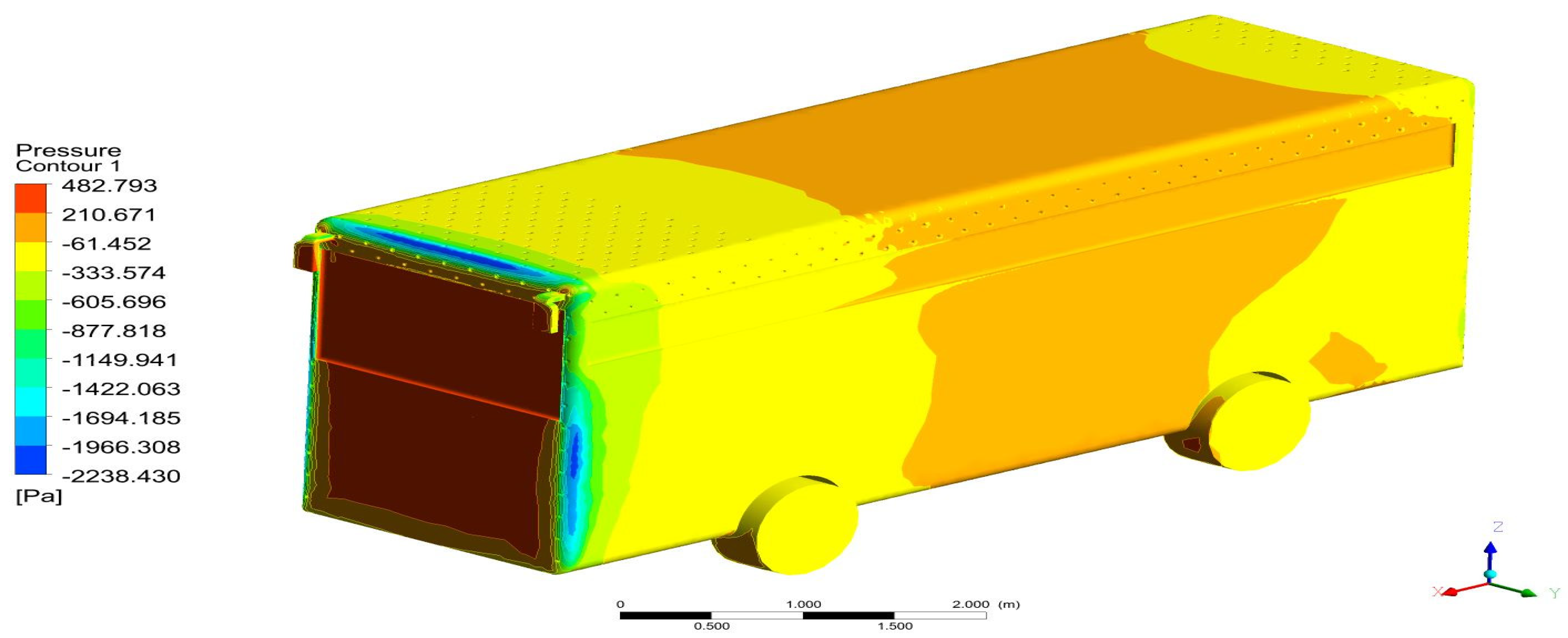
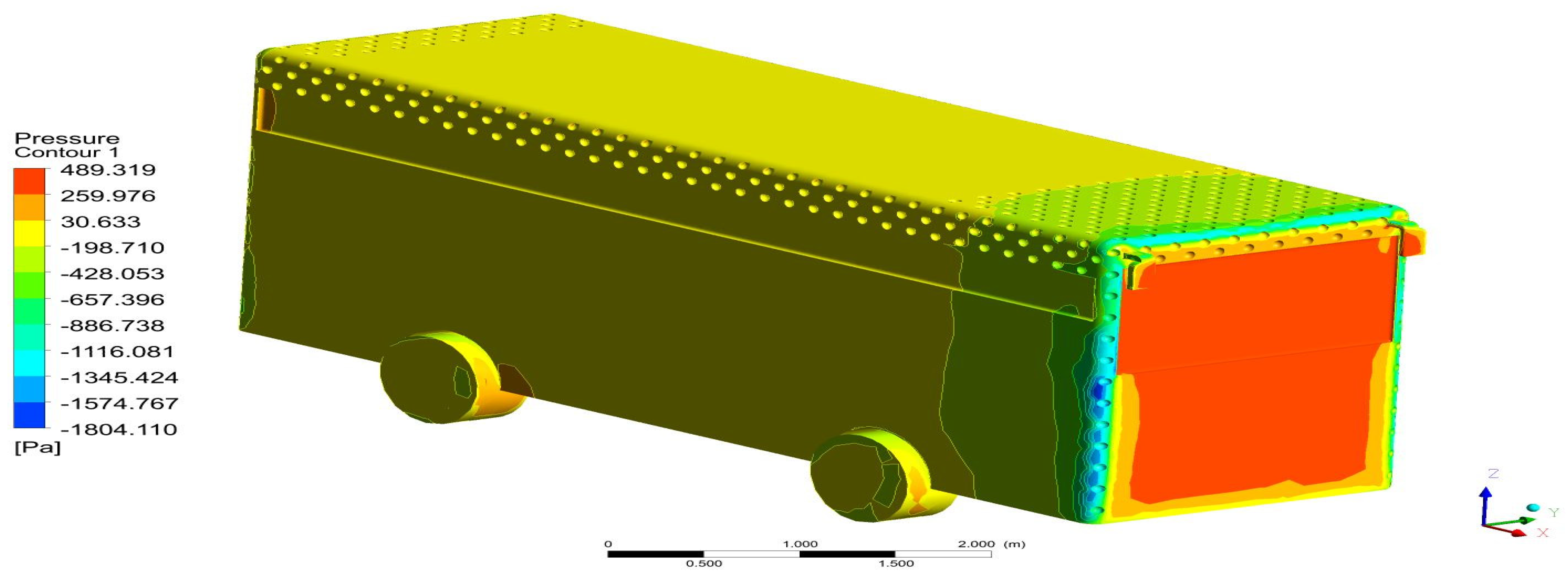
Figure 64.
Aerodynamic pressure variations on the base bus model—isometric view-based representation.
Figure 64.
Aerodynamic pressure variations on the base bus model—isometric view-based representation.
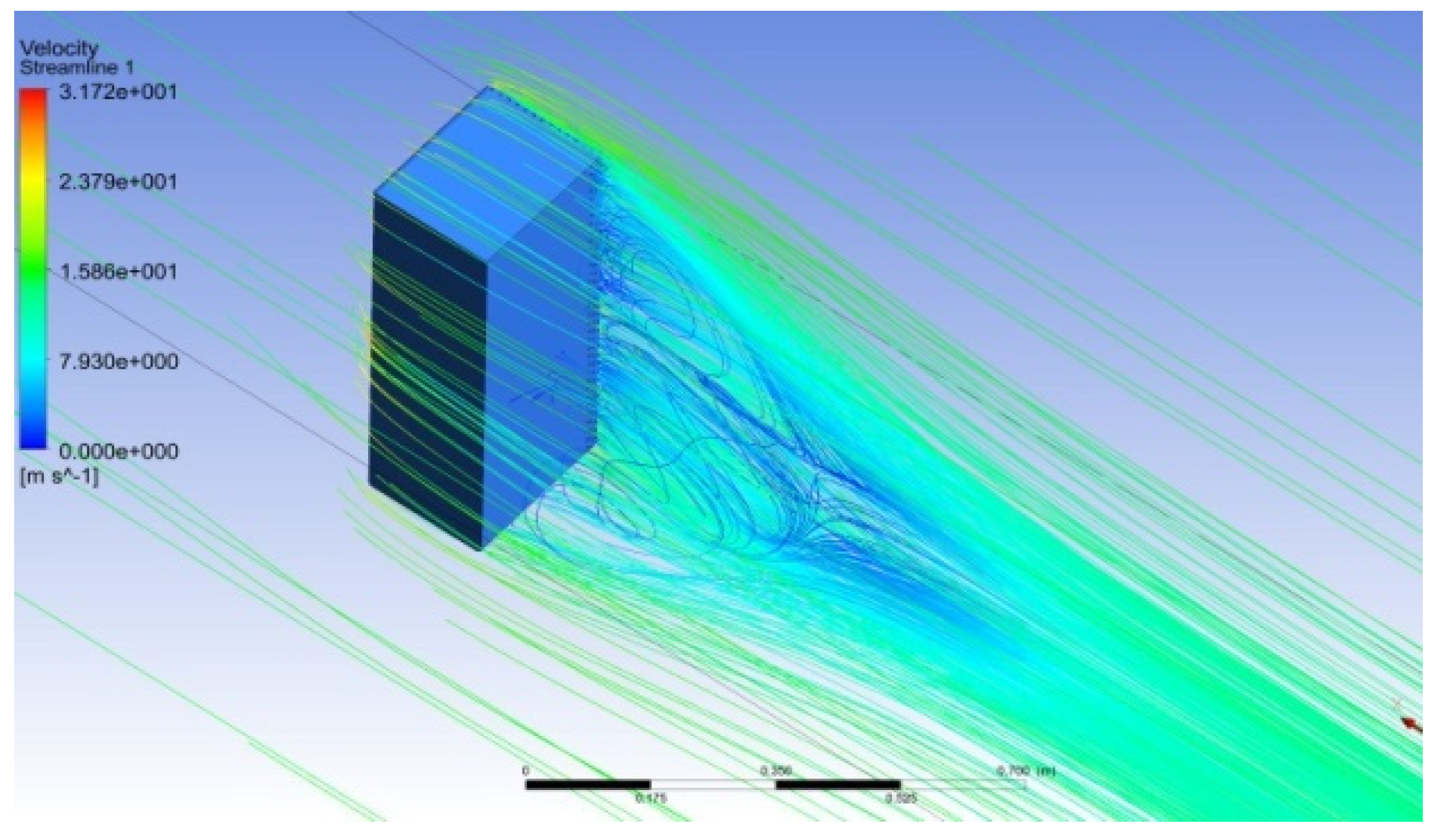
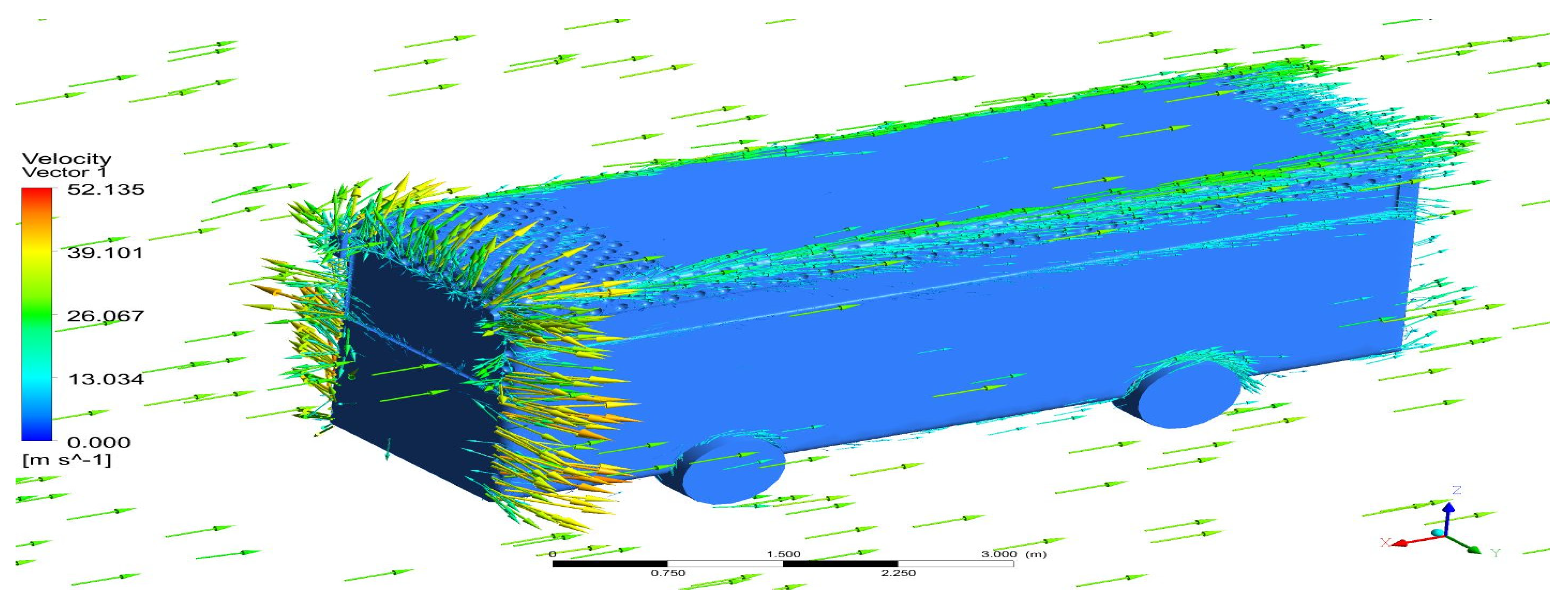
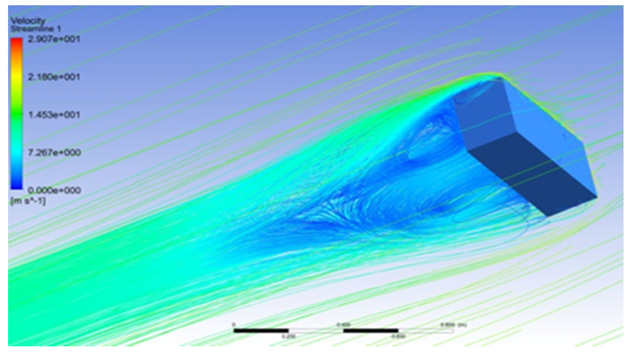
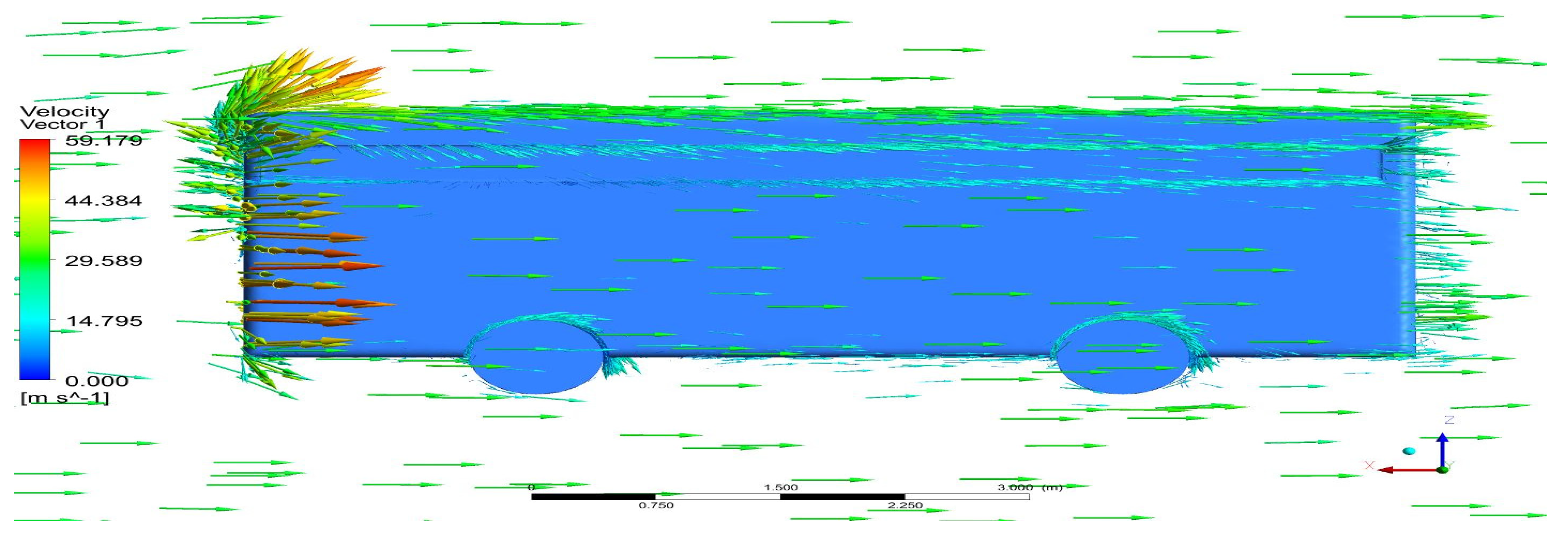
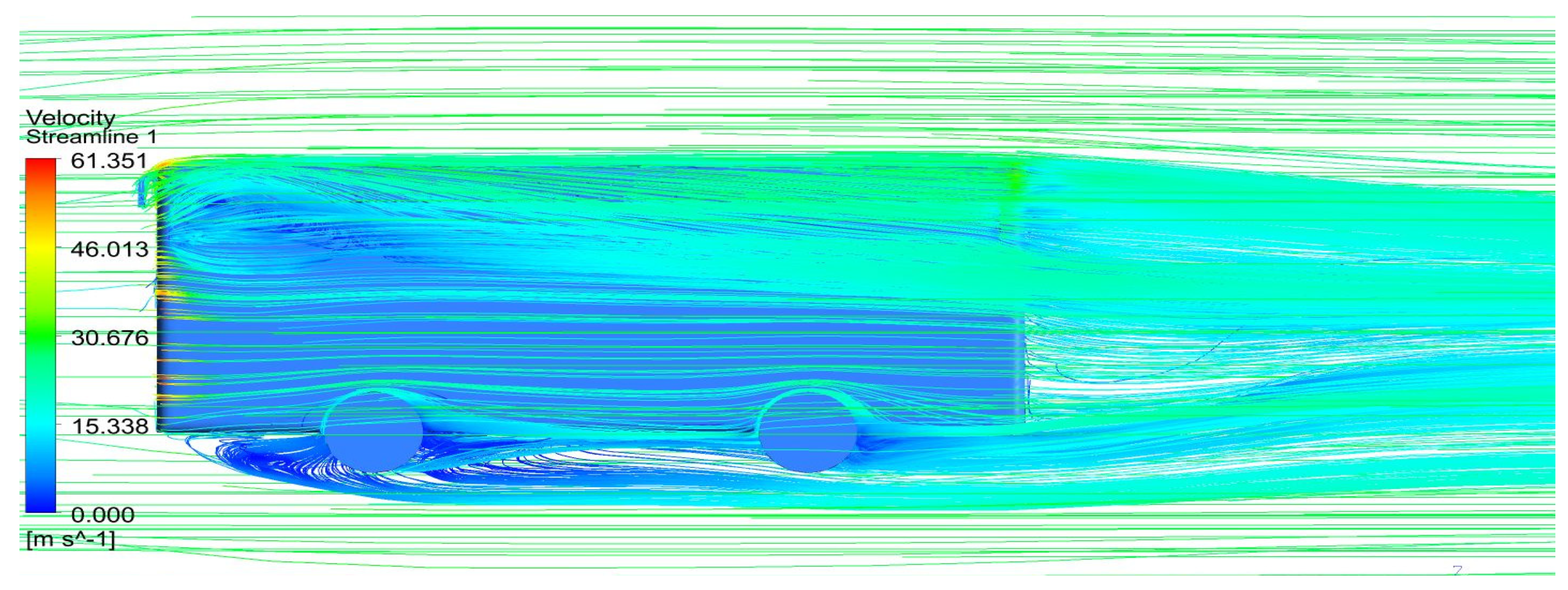
Figure 65.
Aerodynamic fluid velocity variations over the intercity bus through vector-based projections.
Figure 65.
Aerodynamic fluid velocity variations over the intercity bus through vector-based projections.
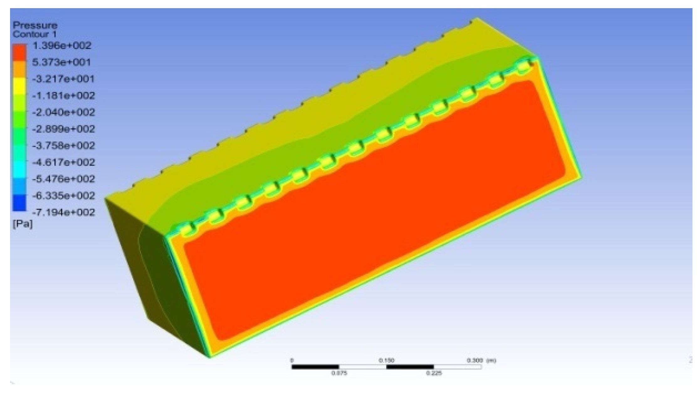
Figure 66.
Typical projection of pressure distributions on the intercity bus loaded with 30 mm dimples.
Figure 66.
Typical projection of pressure distributions on the intercity bus loaded with 30 mm dimples.
Figure 67.
Velocity variations over the intercity bus loaded with 30 dimples through streamline-based projections.
Figure 67.
Velocity variations over the intercity bus loaded with 30 dimples through streamline-based projections.
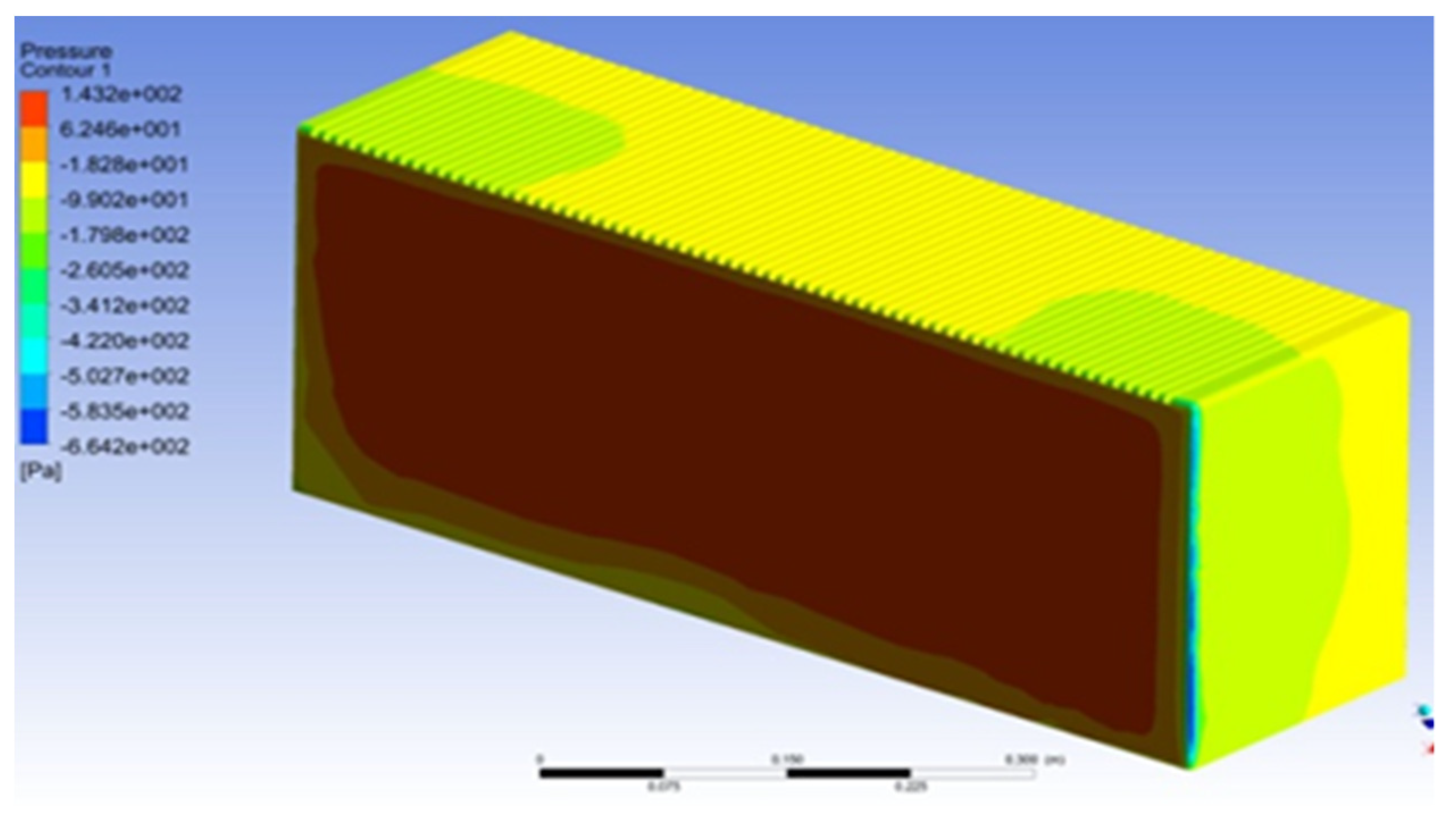
Figure 68.
Aerodynamic pressure variations on the bus model equipped with dimples 50 mm in size—isometric view-based representation.
Figure 68.
Aerodynamic pressure variations on the bus model equipped with dimples 50 mm in size—isometric view-based representation.
Figure 69.
Aerodynamic velocity distributions over the bus model equipped with dimples 50 mm in size—side view-based representation.
Figure 69.
Aerodynamic velocity distributions over the bus model equipped with dimples 50 mm in size—side view-based representation.
Figure 70.
Aerodynamic pressure variations on the bus model equipped with dimples 75 mm in size—isometric view-based representation.
Figure 70.
Aerodynamic pressure variations on the bus model equipped with dimples 75 mm in size—isometric view-based representation.
Figure 71.
Aerodynamic velocity distributions over the bus model equipped with dimples 75 in size—side view-based representations through streamline mode.
Figure 71.
Aerodynamic velocity distributions over the bus model equipped with dimples 75 in size—side view-based representations through streamline mode.
Figure 72.
Aerodynamic pressure variations on the bus model equipped with dimples 100 in size—isometric view-based representation.
Figure 72.
Aerodynamic pressure variations on the bus model equipped with dimples 100 in size—isometric view-based representation.
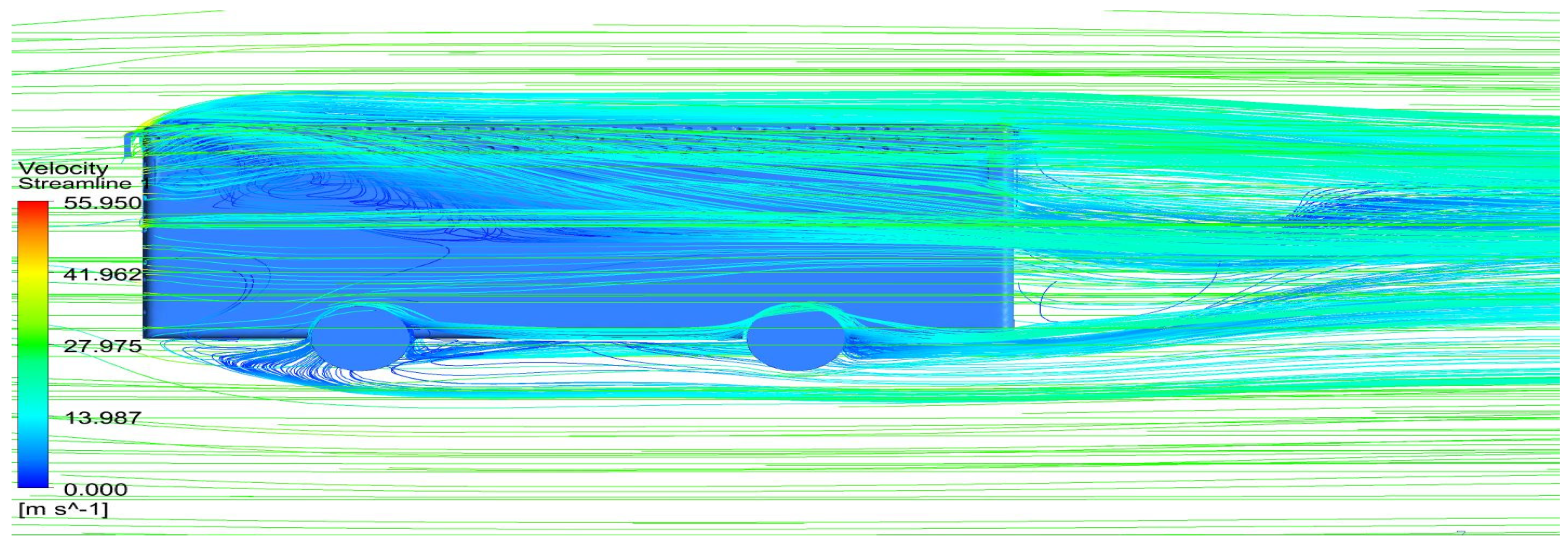
Figure 73.
Velocity variations of the intercity bus loaded with 100 mm dimples at the speed of 100 km/h.
Figure 73.
Velocity variations of the intercity bus loaded with 100 mm dimples at the speed of 100 km/h.
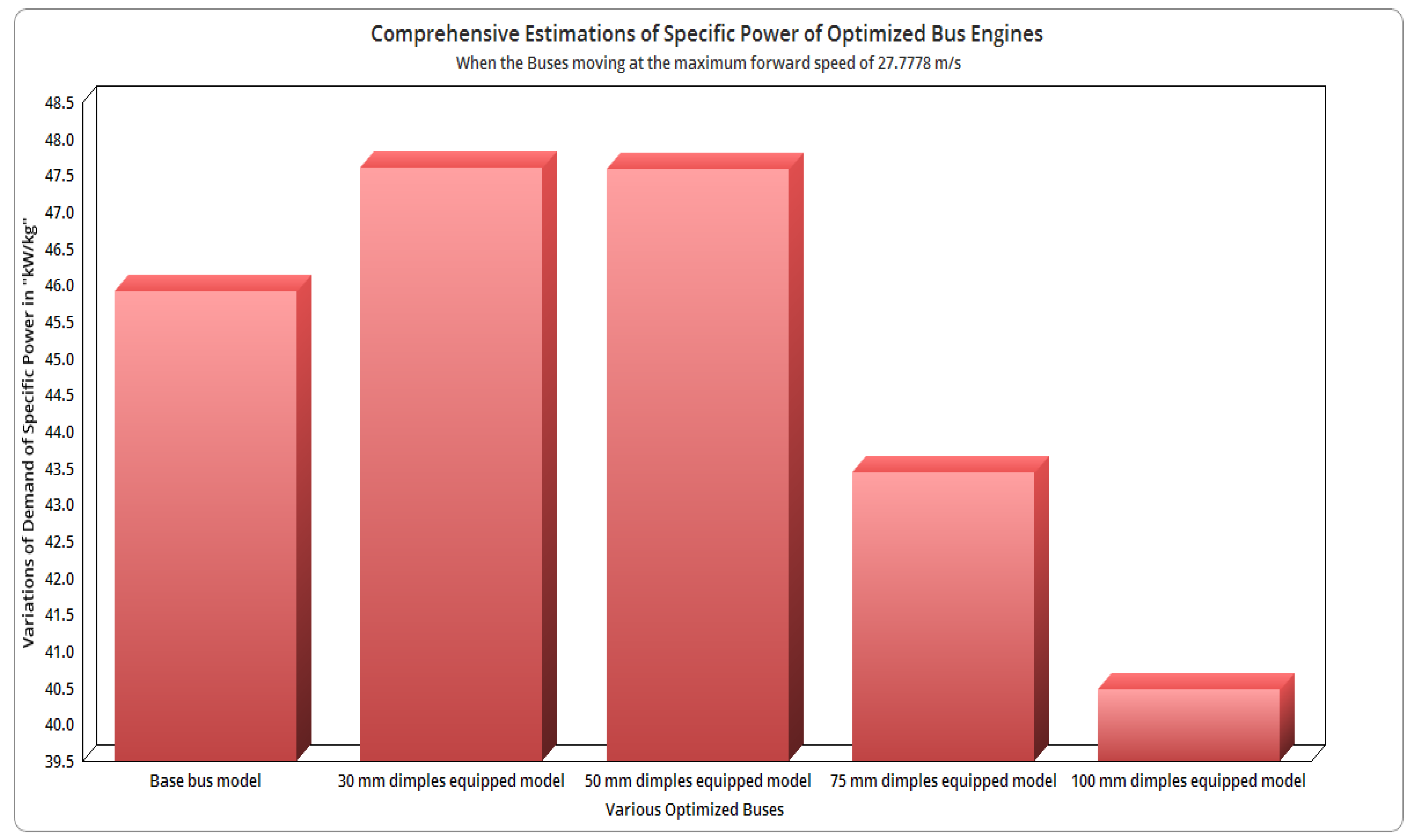
Figure 74.
Comprehensive estimations of specific power of the optimized bus engines.
Figure 74.
Comprehensive estimations of specific power of the optimized bus engines.
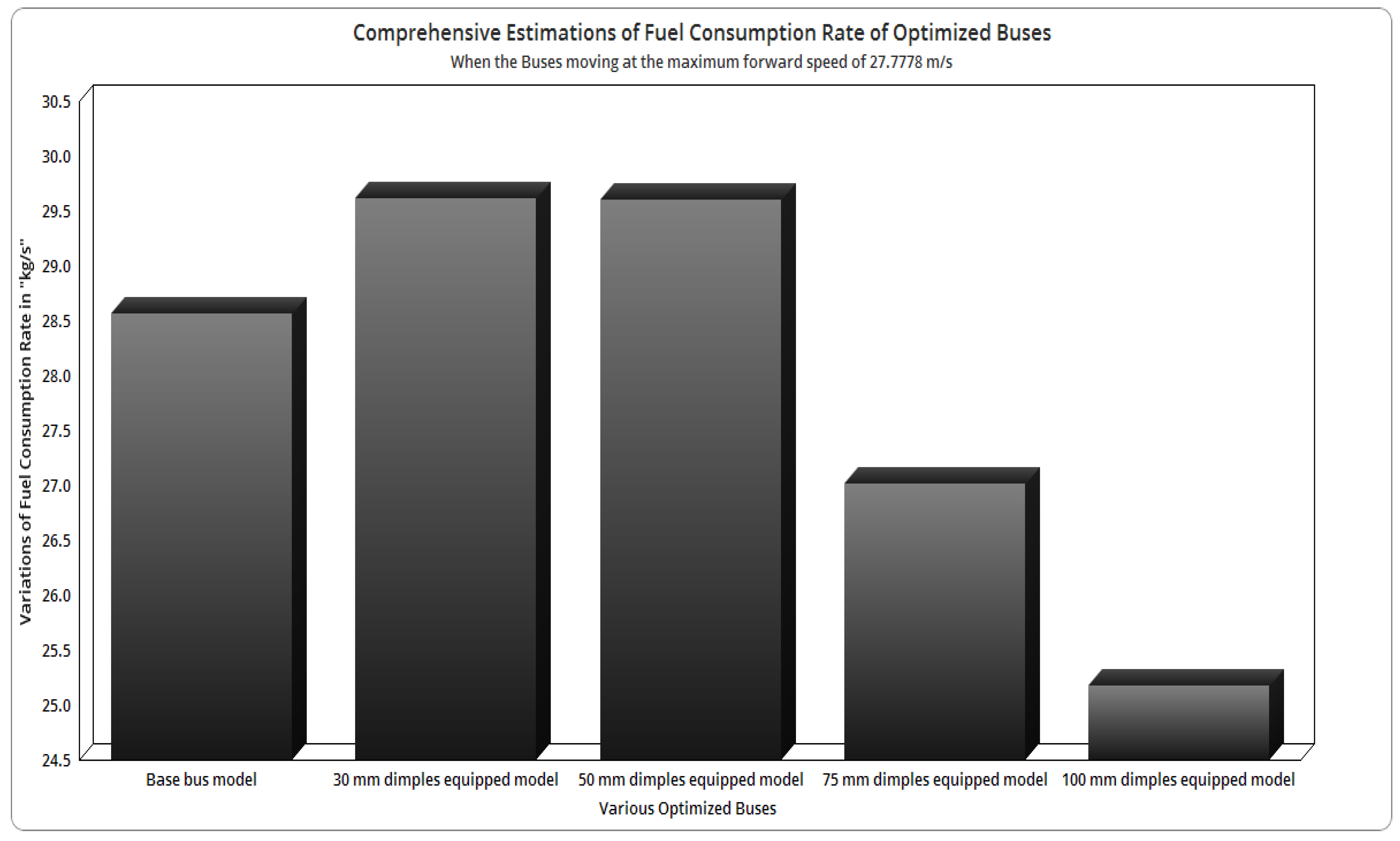
Figure 75.
Comprehensive estimations of the fuel consumption rate of the optimized buses.
Figure 75.
Comprehensive estimations of the fuel consumption rate of the optimized buses.
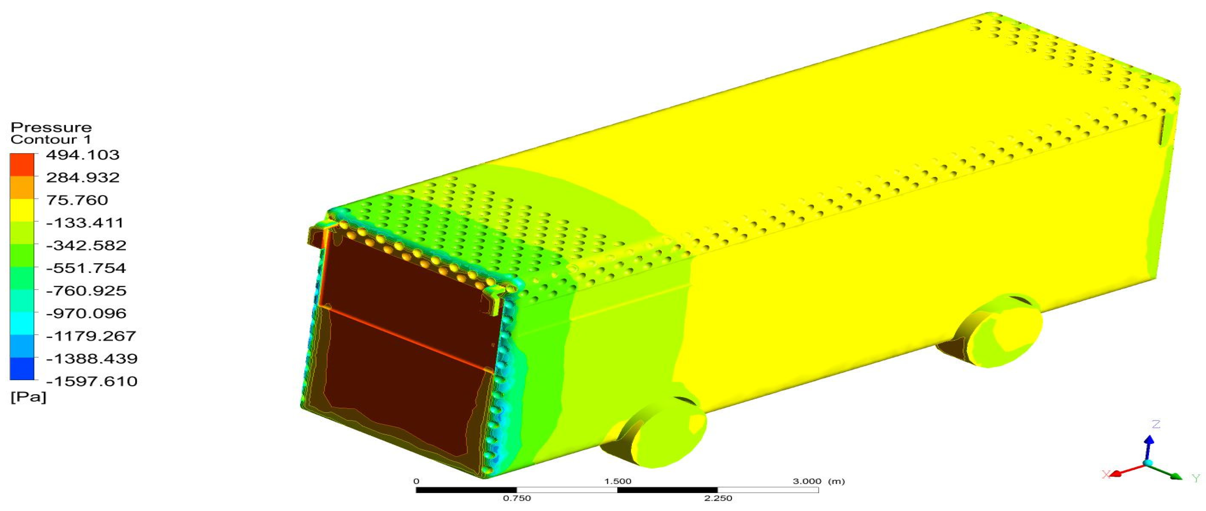
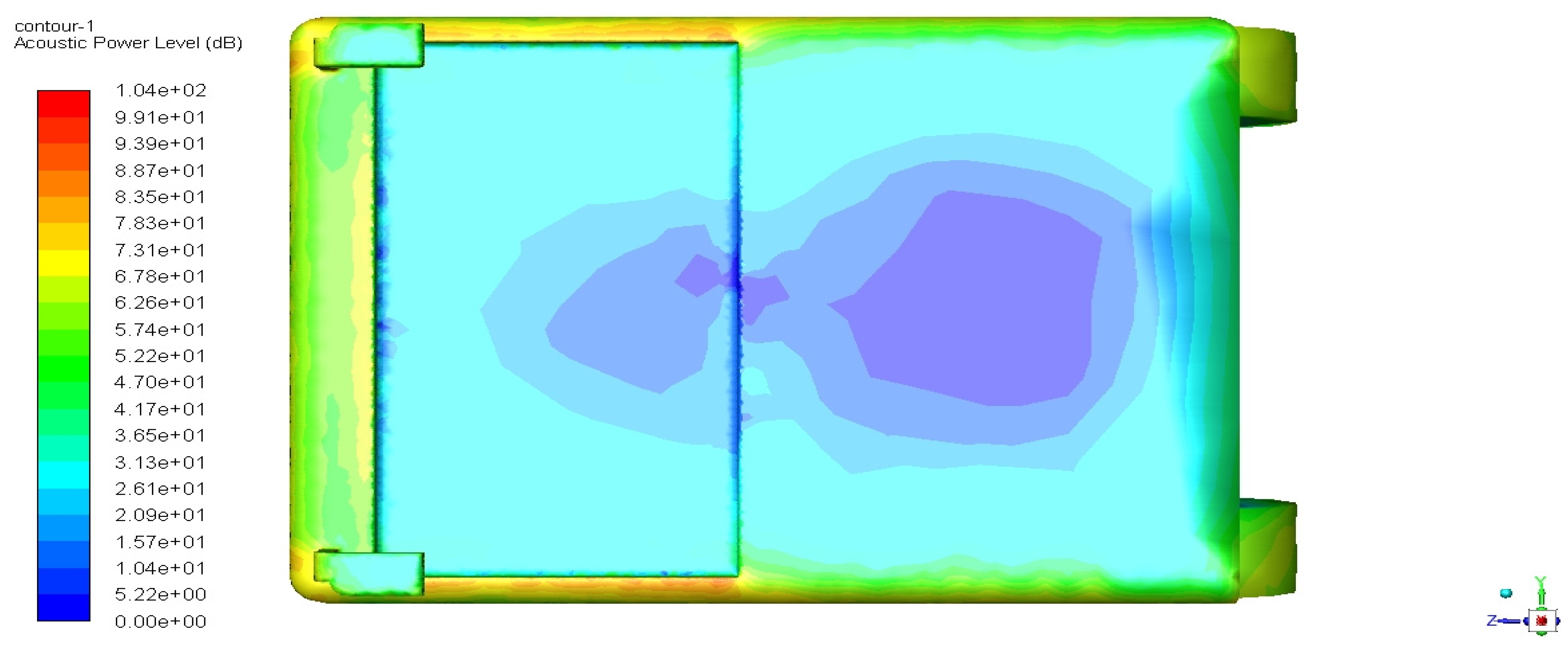
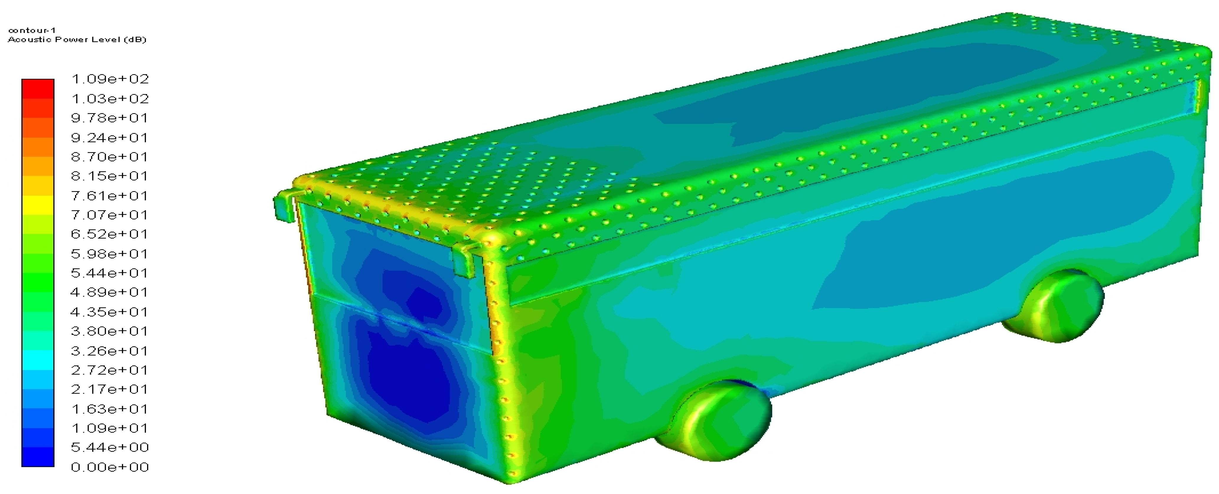
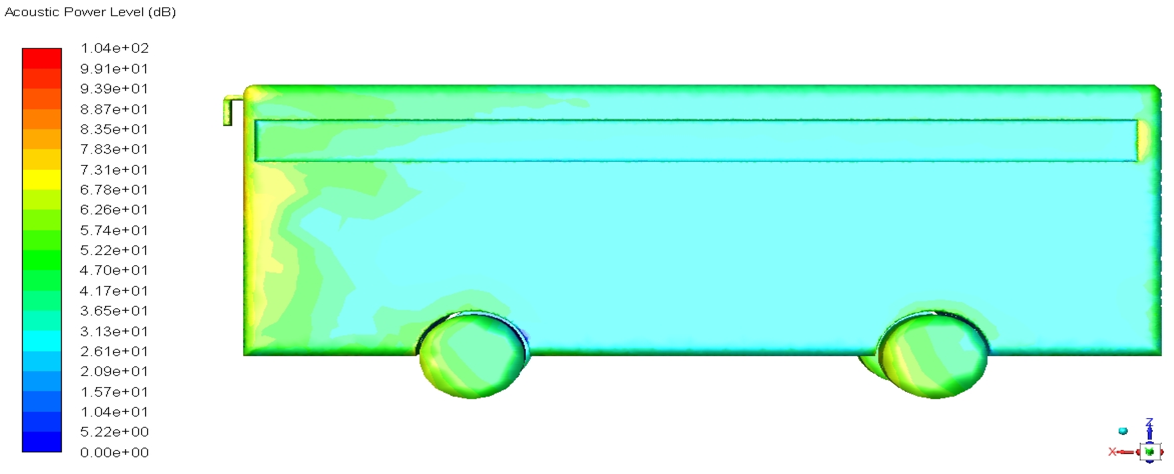
Figure 76.
Typical representation of aeroacoustic outputs of the base bus model—front view.
Figure 76.
Typical representation of aeroacoustic outputs of the base bus model—front view.
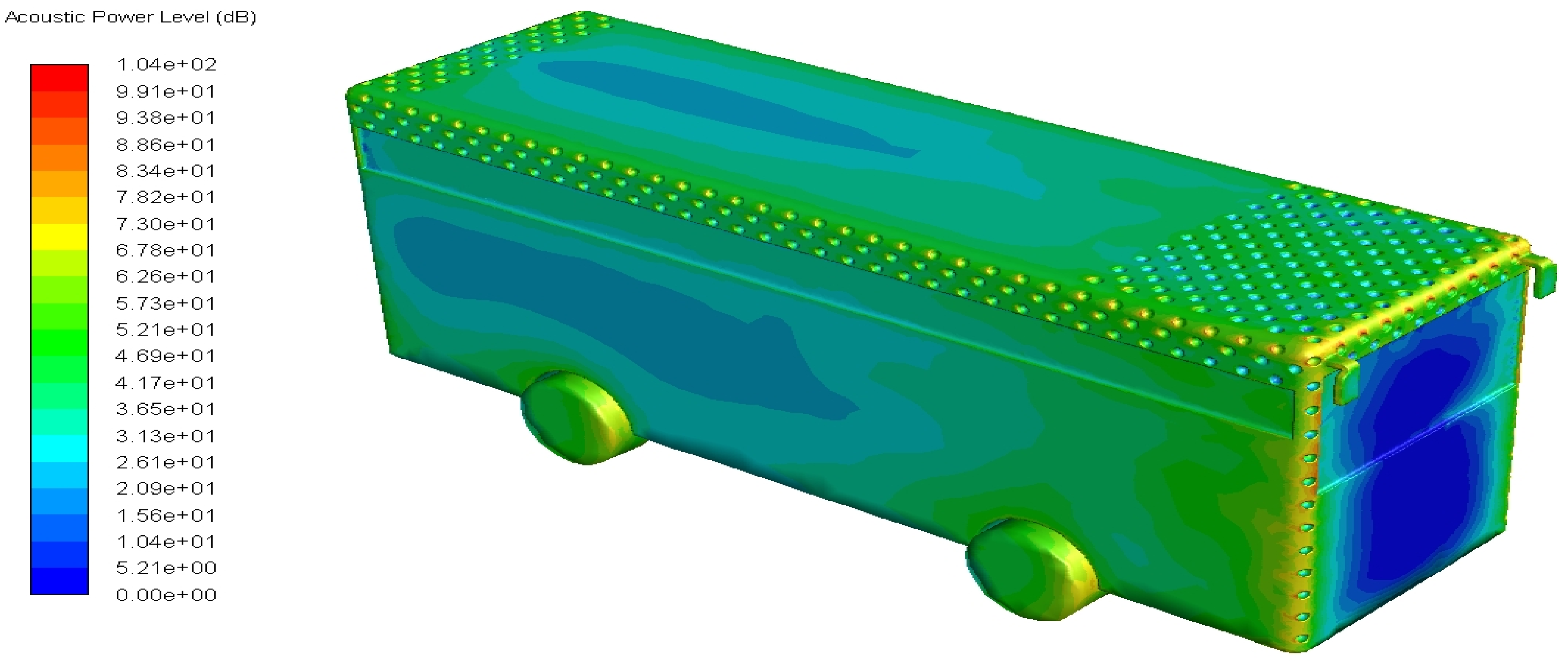
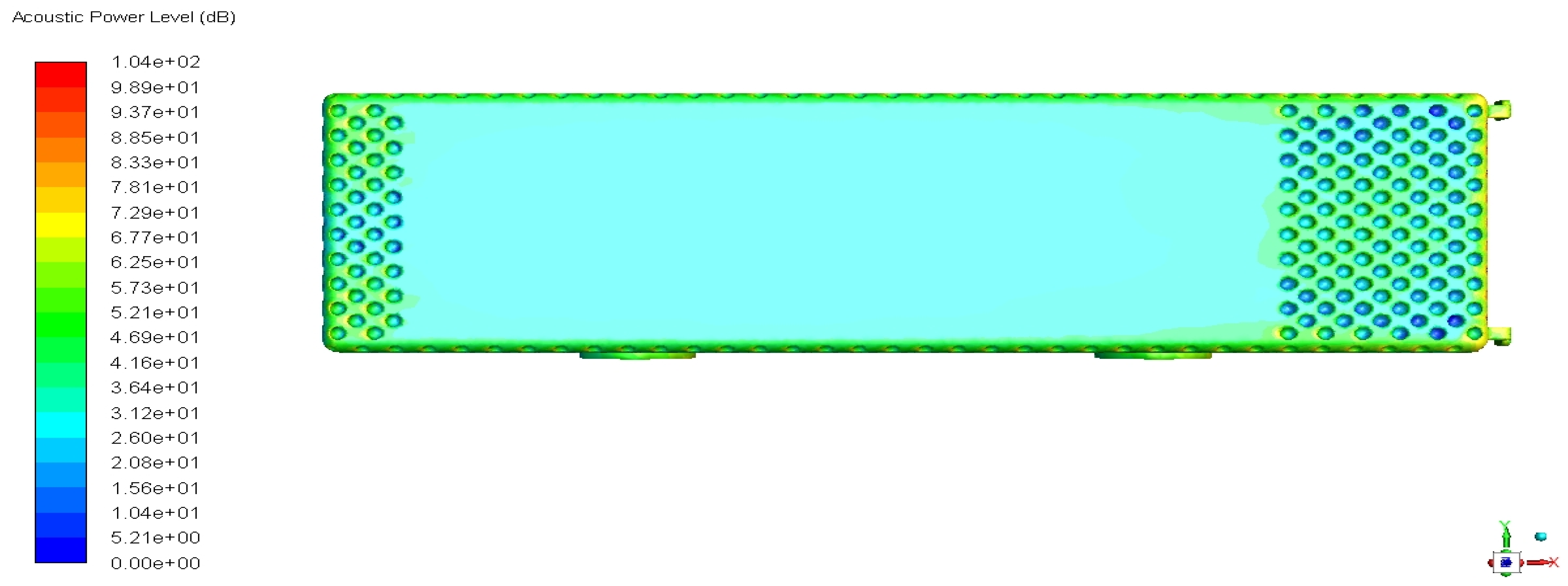
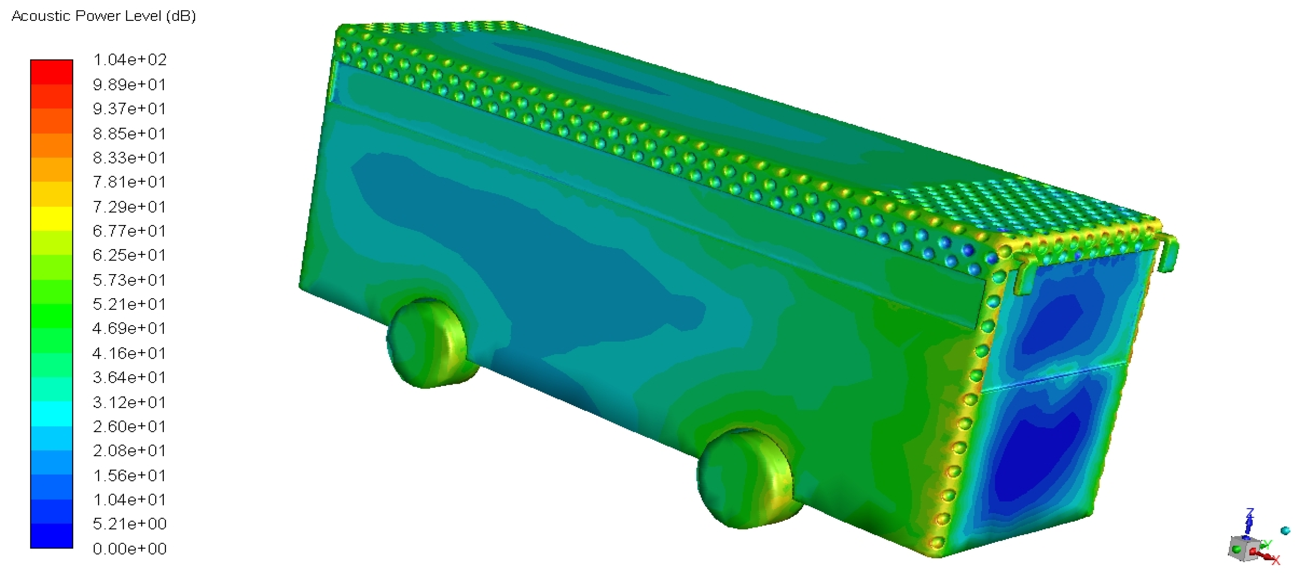
Figure 77.
Typical representation of aeroacoustic outputs of the base bus model—side view.
Figure 77.
Typical representation of aeroacoustic outputs of the base bus model—side view.
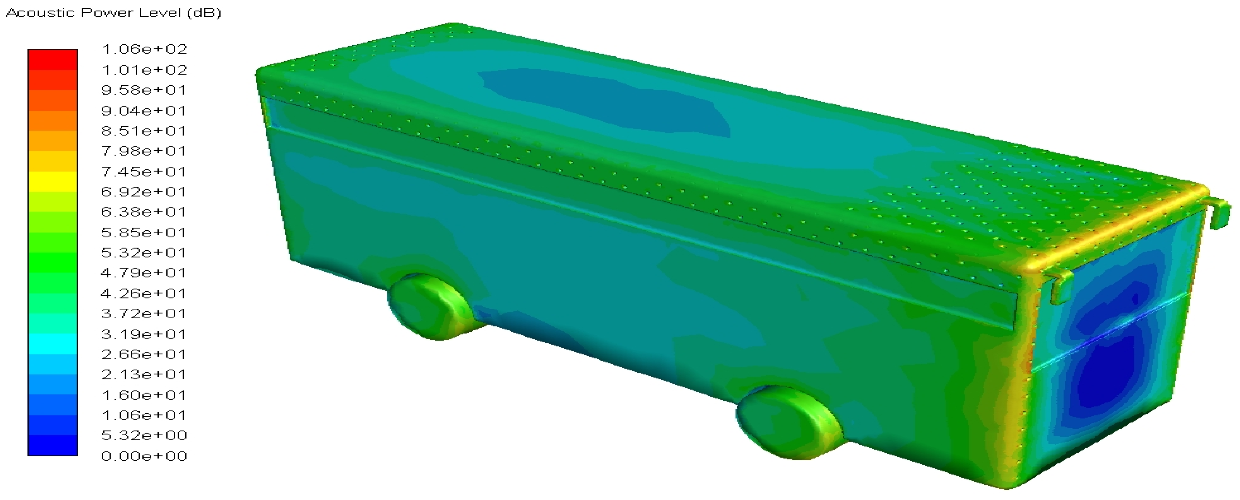
Figure 78.
Typical representation of aeroacoustic outputs of the 30 mm dimple-equipped intercity bus—isometric view.
Figure 78.
Typical representation of aeroacoustic outputs of the 30 mm dimple-equipped intercity bus—isometric view.
Figure 79.
Typical representation of aeroacoustic outputs of 50 mm dimple-equipped intercity bus—isometric view.
Figure 79.
Typical representation of aeroacoustic outputs of 50 mm dimple-equipped intercity bus—isometric view.
Figure 80.
Typical representation of aeroacoustic outputs of 75 mm dimple-equipped intercity bus—isometric view.
Figure 80.
Typical representation of aeroacoustic outputs of 75 mm dimple-equipped intercity bus—isometric view.
Figure 81.
Typical representation of aeroacoustic outputs of 100 mm dimple-equipped intercity bus—top view.
Figure 81.
Typical representation of aeroacoustic outputs of 100 mm dimple-equipped intercity bus—top view.
Figure 82.
Typical representations of aeroacoustic outputs of 100 mm dimple-equipped intercity bus—isometric view.
Figure 82.
Typical representations of aeroacoustic outputs of 100 mm dimple-equipped intercity bus—isometric view.
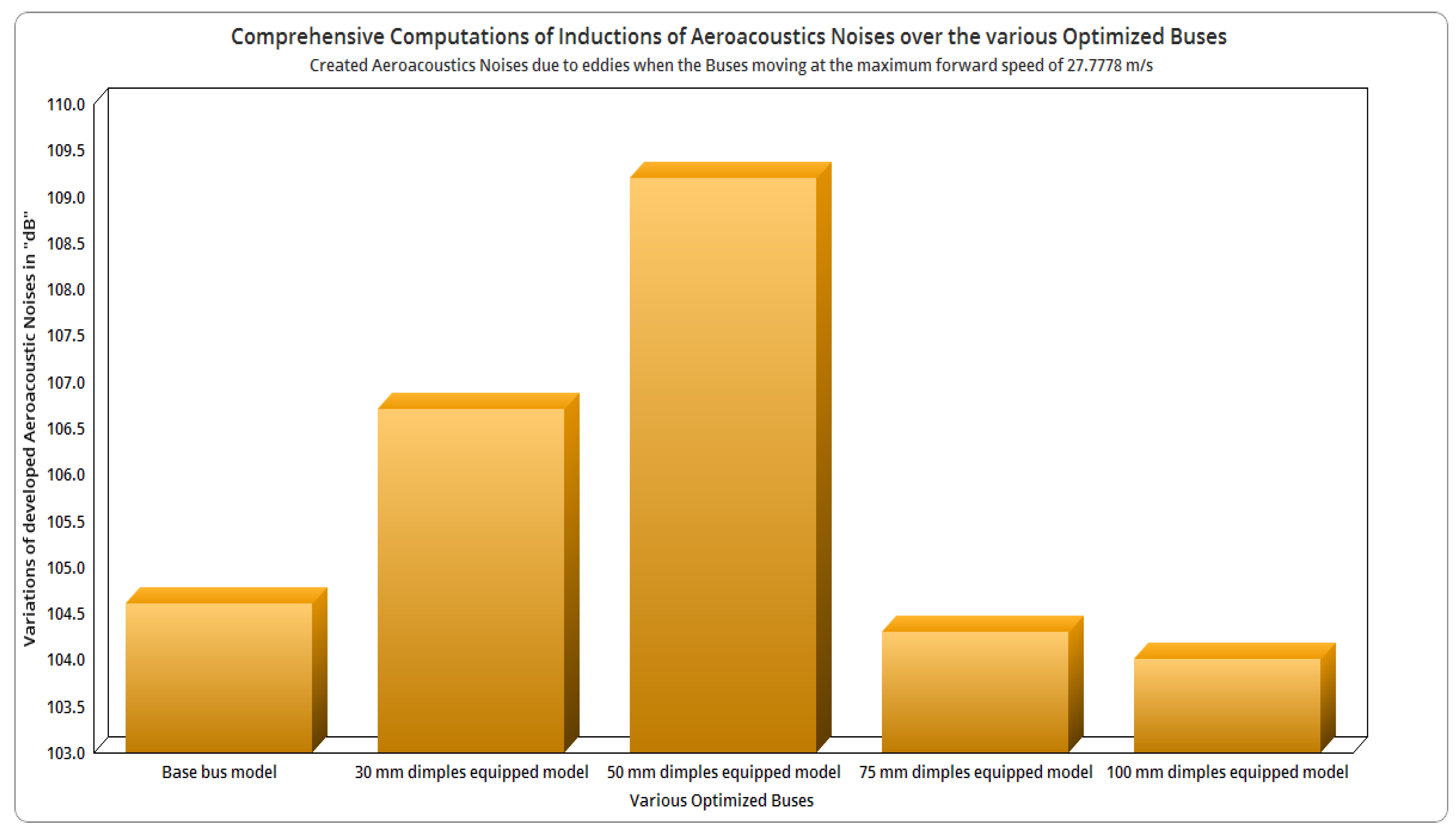
Figure 83.
Comprehensive computations of the inductions of aeroacoustics over the various optimized buses.
Figure 83.
Comprehensive computations of the inductions of aeroacoustics over the various optimized buses.
Table 1.
Comprehensive explanations of various drag reduction techniques.
Table 1.
Comprehensive explanations of various drag reduction techniques.
| Bus Model | Corresponding Figure Number | Description about the Proposed Drag Reduction Techniques |
|---|
| Base model | 2 | The modeled bus is considered the base, so no modifications are imposed on this model. |
| Model I | 3 | A blunt body (outer shape of the bus model) equipped with more dimples on the top and side surfaces |
| Model II | 4 | A blunt body (outer shape of the bus model) equipped with inverted dimples on the top and side surfaces |
| Model III | 5 | A blunt body (outer shape of the bus model) equipped with dimples on the side and top surfaces |
| Model IV | 6 | A blunt body (outer shape of the bus model) equipped with square cuts on the side surface |
| Model V | 7 | A blunt body (outer shape of the bus model) equipped with fins with a gap of 10 mm on the top surface |
| Model VI | 8 | A blunt body (outer shape of the bus model) equipped with fins with a gap of 20 mm on the top surface |
| Model VII | 9 | A blunt body (outer shape of the bus model) equipped with riblets on the top surface |
| Model VIII | 10 | A blunt body (outer shape of the bus model) equipped with dimples on the top surface |
Table 2.
Comparative information of all the mesh cases.
Table 2.
Comparative information of all the mesh cases.
| Types of Meshes | Details of Statics of Mesh |
|---|
| Number of Nodes | Number of Elements |
|---|
| Case 1—coarse mesh | 101,163 | 554,695 |
| Case 2—medium mesh | 252,276 | 1,369,327 |
| Case 3—fine mesh | 523,346 | 2,818,069 |
| Case 4—fine with face mesh set-up | 696,383 | 3,843,318 |
| Case 5—fine with inflation mesh set-up | 643,964 | 3,458,589 |
Table 3.
Comparison of drag on the bus models.
Table 3.
Comparison of drag on the bus models.
| Velocity (m/s) | Drag (N) (Without Dimples) | Drag (N) (With Dimples) |
|---|
| Experimental | Numerical | Error Percentages | Experimental | Numerical | Error Percentages |
|---|
| 14 | 0.26 | 0.2428 | 6.615385 | 0.489 | 0.45 | 7.97546 |
| 17 | 0.59 | 0.394 | 33.22034 | 0.4855 | 0.45 | 7.312049 |
| 20 | 0.7 | 0.67 | 4.285714 | 0.71 | 0.66 | 7.042254 |
| 22 | 1.01 | 0.98 | 2.970297 | 1.01 | 0.996 | 1.386139 |
| 25 | 1.3 | 1.194 | 8.153846 | 1.15 | 1.073 | 6.695652 |
| 28 | 1.37 | 1.2613 | 7.934307 | 1.25 | 1.1973 | 4.216 |
| 35 | 1.695 | 1.55 | 8.554572 | 1.6 | 1.56 | 2.5 |
Table 4.
Comprehensive outcome of drag generated on various bus models—forward direction.
Table 4.
Comprehensive outcome of drag generated on various bus models—forward direction.
| Bus Model | Upward Force (N) | Sideslip Force (N) | Drag Force (N) |
|---|
| Base model | 1.10147 | 0.29927 | 7.037 |
| Model I | 0.0660117 | 0.356574 | 5.76606 |
| Model II | 0.0616214 | 0.0105042 | 9.83527 |
| Model III | 1.82655 | 0.450884 | 7.49661 |
| Model IV | 0.212934 | 0.4451 | 6.5703 |
| Model V | 0.236562 | 0.0588171 | 12.0567 |
| Model VI | 0.13367 | 0.248186 | 11.836 |
| Model VII | 0.270574 | 0.640371 | 6.93219 |
| Model VIII | 1.1323 | 0.209187 | 7.0459 |
Table 5.
Comparison of side forces on various bus models.
Table 5.
Comparison of side forces on various bus models.
| Intercity Bus Models | Side Force Value in “Newton” |
|---|
| Crosswind Velocity (5 m/s) | Crosswind Velocity (10 m/s) | Crosswind Velocity (15 m/s) |
|---|
| Base model | 2.40392 | 9.18491 | 20.2098 |
| Model I | 1.35382 | 6.41537 | 13.7896 |
| Model II | 2.71512 | 11.3569 | 25.3571 |
| Model III | 1.42998 | 6.6384 | 14.2063 |
| Model IV | 1.39427 | 9.72601 | 21.5342 |
| Model V | 3.08994 | 12.4983 | 28.2582 |
| Model VI | 3.03373 | 12.4949 | 27.9074 |
| Model VII | 2.93207 | 13.1211 | 29.4811 |
| Model VIII | 1.30671 | 5.95073 | 12.8353 |
Table 6.
Comprehensive aerodynamic forces on and over the optimized civilian intercity buses.
Table 6.
Comprehensive aerodynamic forces on and over the optimized civilian intercity buses.
| Bus Models | Drag (FD) (N) | Upward Force (N) | Side Slip Force (N) | Induced Velocity (m/s) |
|---|
| Base bus model | 1560.44 | 23.9324 | 114.237 | 59.179 |
| 30 mm dimple-loaded bus model | 1550.41 | 0.940451 | 80.7699 | 61.351 |
| 50 mm dimple-loaded bus model | 1574.78 | 42.3091 | 36.5971 | 61.330 |
| 75 mm dimple-loaded bus model | 1806.74 | 30.8007 | 49.8049 | 55.950 |
| 100 mm dimple-loaded bus model | 1904.09 | 16.3635 | 57.0211 | 52.135 |
Table 7.
Comprehensive estimated data of required energy and its associates of the optimized civilian intercity buses.
Table 7.
Comprehensive estimated data of required energy and its associates of the optimized civilian intercity buses.
| Bus Models | FRR (N) | FD (N) | FIB (N) | FA (N) | ER (W) |
|---|
| Base bus model | 1481.814 | 1560.44 | 564,151.1735 | 138.1694 | 18,114,050.15 |
| 30 mm dimple-loaded bus model | 1481.736 | 1550.41 | 564,121.3957 | 81.71035 | 18,110,974.01 |
| 50 mm dimple-loaded bus model | 1481.345 | 1574.78 | 563,972.5067 | 78.9062 | 18,106,896.28 |
| 75 mm dimple-loaded bus model | 1480.21 | 1806.74 | 563,540.7286 | 80.6056 | 18,100,534.41 |
| 100 mm dimple-loaded bus model | 1478.294 | 1904.09 | 562,811.1725 | 73.3846 | 18,080,057.28 |


 ,
, 


