Abstract
Buildings are currently among the largest consumers of electrical energy with considerable increases in CO2 emissions in recent years. Although there have been notable advances in energy efficiency, buildings still have great untapped savings potential. Within demand-side management, some tools have helped improve electricity consumption, such as energy forecast models. However, because most forecasting models are not focused on updating based on the changing nature of buildings, they do not help exploit the savings potential of buildings. Considering the aforementioned, the objective of this article is to analyze the integration of methods that can help forecasting models to better adapt to the changes that occur in the behavior of buildings, ensuring that these can be used as tools to enhance savings in buildings. For this study, active and passive change detection methods were considered to be integrators in the decision tree and deep learning models. The results show that constant retraining for the decision tree models, integrating change detection methods, helped them to better adapt to changes in the whole building’s electrical consumption. However, for deep learning models, this was not the case, as constant retraining with small volumes of data only worsened their performance. These results may lead to the option of using tree decision models in buildings where electricity consumption is constantly changing.
1. Introduction
Buildings presently produce up to 40% of worldwide energy consumption and 30% of carbon dioxide emissions, numbers which are constantly increasing due to urbanization [1]. Additionally, considering the long life expectancy of buildings, it is assessed that 85–95% of buildings that exist today will still be utilized in 2050 [2]. Hence, changes in energy utilization on buildings are inclined to intensely affect current society, including major economic and environmental changes such as climate change and global warming [3,4]. Buildings are becoming substantially more complex and sophisticated. They integrate conventional energy services systems, on-site energy generation systems, and charging systems [5]. For this reason, energy management is becoming fundamental for buildings around the world, and energy forecasting is essential as an initial step to establish an energy management system [6]. The forecasting of building energy utilization supports smart building performance through low energy and control procedures [7].
In recent times, because of their important application in various fields including electric energy consumption in buildings, data-driven models such as machine- and deep learning-based approaches have become exceptionally well known [8] and are being utilized to improve forecast accuracy [9]. In real life, electrical consumption forecasting models should regularly be made online in real-time. An online setting brings extra challenges since there could be an anticipation of changes to the information distribution over the long haul [10]. However, traditional electric energy forecasting models are normally trained once and not re-trained again with new data, thus missing out on the new information that new data can provide [11]. When this situation happens, it can lead to incorrect forecasting [12].
Recognizing change points and incorporating these uncertain change points into electric energy forecasting models is one of the most difficult tasks [13]. The unexpected changes in the data distribution over time, are known as concept drift [14]. Concept drift has been perceived as the root cause of decreased effectiveness in data-driven decision support systems [15]. Based on how the data change, concept drift can be separated into different kinds: sudden, gradual, recurring, and incremental [16]. Sudden drift happens when the data change quickly and without variation. Whenever the data begin changing in class distribution, this is defined as gradual drift. Recurring drifts happen when the data change for a moment and then return sooner or later. Incremental drift occurs when the data continuously change over the long run [17].
To address those different situations in forecasting models, two main strategies have been used: active and passive methods. For active methods, a model is equipped with a change detection strategy and re-trained when a trigger has been flagged. Nonetheless, in passive methods, algorithms are re-trained at regular intervals regardless of whether a change has occurred or not [18]. There has been a very important effort investigating concept drift in regression tasks (see Table 1) that have focused on load forecasting in houses [19,20], energy consumption in smart grids [21], electricity supply and demand [22], total reactive power [23], energy production for a wind farm [24], power generation in a photovoltaic plant [25], and electricity price [26,27]. However, there have not been many works in real cases where concept drift techniques are used to maintain or improve the results of machine learning techniques in smart buildings. Therefore, this paper’s objective is to provide a novel analysis of the integration of drift detection methods in decision trees and deep learning algorithms for whole building electricity consumption forecasting in smart buildings.

Table 1.
Summary of literature review, their contributions, and their limitations.
Given the above, the main contributions of this paper in this field of research could be summarized as follows:
- Integration of drift detection methods to a multi-step forecasting strategy that forecasts the next 24 h from any hour of the day.
- An analysis of the integration of drift detection methods in decision trees and deep learning algorithms for forecasting the electricity consumption of the entire building.
- Comparison analysis between active and passive drift detection methods for building electricity consumption forecasting in smart buildings.
2. Methodology and Approach
The use of drift detection methods is well known, however, the integration of these methods into a multi-step forecasting strategy to predict continuous hourly electricity energy consumption in the entire building turns out to be a novel topic.
Therefore, this section describes data preprocessing, forecasting algorithms, drift detection methods, and performance metrics used in this article. Section 2.1 provides information on how the datasets from the two buildings used to train the learning algorithms were made. Section 2.2 presents the approach and the learning algorithms used to forecast the electrical consumption in buildings. Section 2.3 describes the drift detection methods and their incorporation into the learning algorithms. Section 2.4 explains the metrics used for evaluating the performance of learning algorithms. A summary of the methodology used is shown in Figure 1.
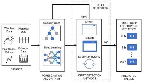
Figure 1.
Methodology used for the analysis of the integration of drift detection methods.
2.1. Datasets Construction
For this research, the data from two buildings located on the campus of the University of Valladolid were used. These data were obtained through smart meters installed in each of the buildings at their electrical power transformer stations, which record the active energy consumed (kWh) of the entire building in intervals of 15 min from 2016 to 2019. At the time of analyzing the data, some missing records were found, because these missing records did not exceed 0.5% of the total value of the data and were not found consecutively, a line interpolation technique was applied to complete these missing records. After completing the missing data, since it was desired to forecast the electricity consumption per hour, the data were conditioned to have the consumption per hour for each building.
Based on previous studies [29,30,31,32,33] where it has been proven that the use of weather, calendar variables, and past values data can help improve the training of learning algorithms, these were included in the datasets. To obtain the past values data, the autocorrelation and partial autocorrelation of the energy consumption variable were analyzed, resulting in a significant autocorrelation up to lag 25. For calendar variables, the timestamps of the historical data were used to obtain the variables of the hour, day, month, and year. Additionally, a variable was added to indicate when it is a working day or not, this variable was made based on the annual calendar of the university. The weather variables that were used were those that are related to the comfort of the occupants inside the building, such as relative humidity, precipitation, minimum temperature, average temperature, maximum temperature, heating degree days, cooling degree days, and all-sky surface longwave downward irradiance. The weather data were obtained from the NASA Langley Research Center (LaRC) POWER Project funded through the NASA Earth Science/Applied Science Program (https://power.larc.nasa.gov/, accessed on 16 March 2022).
2.2. Approach and Forecasting Algorithms
For the electricity consumption forecast, a multi-step forecasting strategy was used, which in this case can predict electricity consumption for the next 24 h from one hour. The advantage of this strategy is that it allows electricity consumption forecasting from any hour of the day, the disadvantage is that it is necessary to prepare the dataset with past values data so that this information can be used by the learning algorithms to forecast the multiple hours more accurately.
Based on studies where decision tree [34,35,36,37] and deep learning algorithms [38,39,40,41] obtained good results in forecasting electrical consumption in buildings, two decision trees, and two deep learning algorithms were selected. From the decision tree algorithms, Random Forest (RF) and eXtreme Gradient Boosting (XGBoost) were selected, while from the deep learning algorithms, Convolutional Neural Network (CNN), and Temporal Convolutional Network (TCN) was chosen. The architectures of the learning algorithms used are shown in Figure 2.
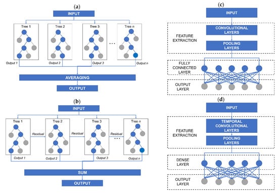
Figure 2.
(a) Basic RF architecture. (b) Basic XGBoost architecture. (c) Basic CNN architecture. (d) Basic TCN architecture.
The algorithms used were programmed in Python using the Scikit-learn, XGBoost, Keras, and TensorFlow libraries. To obtain the best combination of hyperparameters and architecture for the algorithms, backtesting with sliding windows was used. The backtesting with sliding windows procedure consisted of keeping the same training size and sliding a data window to create five different training tests (see Figure 3). For this case, the data from 2016 to 2017 were used for the training set, while the data from 2018 were used for the validation sample. Once the best architecture and parameters were defined through backtesting, the model was adjusted with data from 2016 to 2018, leaving 2019 as the testing set. The best combinations of parameters obtained in the backtesting process are shown in Table 2. The parameters that do not appear in the table are absent because their default values were used.
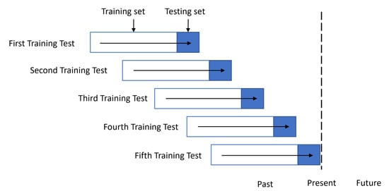
Figure 3.
Backtesting with sliding windows procedure.
Table 2.
Best combinations of parameters obtained through backtesting procedure.
2.3. Drift Detection Methods
Since the selected algorithms are not capable of detecting changes in the data distribution, two well-known active drift detection methods (DDM), Adaptive Window (ADWIN) and Kolmogorov–Smirnov Window (KSWIN) [28] were incorporated into them. These methods were selected because the training uses the latest batch of data with the latest training instances and the size of the window is generally determined by the user.
ADWIN accurately keeps a variable-length window of late values; to such an extent that it holds that there has not been a change in the data distribution. This window is additionally isolated into two sub-windows (W0, W1) used to decide whether a change has occurred. ADWIN contrasts the median of W0 and W1 to affirm that they coincide with a similar distribution. Concept drift is identified assuming the distribution correspondence does not hold anymore. After recognizing a drift, W0 is changed by W1 and a new W1 is introduced. ADWIN utilizes a certainty value to decide whether the two sub-windows coincide with a similar dispersion [42].
KSWIN is a drift detection method based on the Kolmogorov–Smirnov (KS) measurable test. KS-test is a measurable test without really any suspicion of basic information appropriation. KSWIN keeps a sliding window of fixed size (window_size). The last (stat_size) tests of are accepted to address the last idea considered as . From the main examples of , tests are consistently drawn, addressing an approximated last concept . The KS-test is performed on the windows also , of a similar size. KS-test looks at the distance of the observational aggregate data distribution [27].
A sudden change is distinguished by KSWIN if:
where is the probability for the test statistic of the KS-test, and is the size of the statistic window.
The reason for using methods based on window size was because the training utilizes the last batch of data with the last training set. The window of fixed size approach is the least complex rule and the window size is usually decided by the user. By having data on the time size of the change, a window of the fixed size approach is a valuable decision [11].
2.4. Performace Metrics
To analyze the integration of the DDM, in addition to using active methods, it was proposed to use a passive method, which consisted of retraining the algorithms every 24 h regardless of whether there was a change in the data distribution. These methods were compared in each of the algorithms using performance metrics, mean absolute percentage error (MAPE), mean absolute error (MAE), root mean square error (RMSE), and coefficient of determination (R2) were used.
MAPE shows the measure of the precision of the estimated values comparative with the real values (in a percentage) [43], which is determined according to Equation (2).
MAE is utilized to assess how close estimates or expectations are to the real results. It is determined by averaging the absolute differences between the expected values and the real values [44], as shown in Equation (3).
RMSE evaluates the differences between the real values and estimated values [45], which is determined according to Equation (4):
R2 is a statistical measure of the variance between estimated values acquired by the model and real values (level of direct relationship among anticipated and estimated values) [46], which is determined according to Equation (5).
where is the expected value, is the real value, is the average value, and is the total number of estimations.
The reason why these metrics were chosen was to have an overview of the performance of the models. In the case of the MAPE, it was chosen because it is easy to understand since it presents percentage values, but due to its limitations, it was decided to accompany it with the MAE, which shows how much inaccuracy is expected from the forecast on average, helping to determine which models are better. However, because the MAE can have difficulty distinguishing large from small errors, it was combined with the RMSE to be on the safe side. As for R2, it was selected to know how the data fit the models.
3. Experimentation Setup
Two buildings with a continental Mediterranean climate were selected for testing. These buildings have a lighting and air conditioning control system, as well as an energy monitoring system to provide a balance between the comfort of the occupants and the consumption of electrical energy. The first building corresponds to the Faculty of Science of the University of Valladolid located at coordinates 41.663411°, −4.705539°, which is dedicated to administrative offices, while the second building corresponds to the Faculty of Economics located at coordinates 41.658586°, −4.710667°, which is dedicated to teaching activities. These buildings were selected due to their different behavior in electricity consumption during the selected years. In case of Building 1, it has had changes in consumption only in specific periods, while Building 2 has had a decrease in energy consumption gradually each year because energy efficiency improvements were made, and solar panels were integrated into the building (see Figure 4). The energy source used for Building 1 comes from the electrical grid, while for Building 2, the energy source comes from the electrical grid and photovoltaic panels.
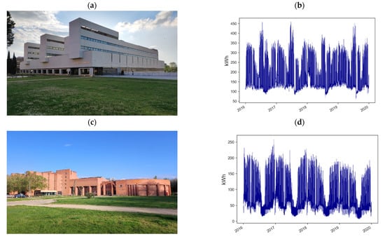
Figure 4.
(a) View of Building 1. (b) Hourly electricity consumption for Building 1. (c) View of Building 2. (d) Hourly electricity consumption for Building 2.
The records of the electrical consumption that were used to test the proposed method were from 2016 to 2019. For the training stage, the years 2016 to 2018 were used, while for the test stage the year 2019 was used. To evaluate the learning algorithms with the DDM, two Python scripts were developed, one for the decision tree algorithms and the other for the deep learning algorithms. Two functions were created in the scripts, the first for updating the algorithms with a passive method and the second for updating with the active methods. In the passive method, the algorithms were retrained every 24 h over a period of one year, while in the active methods, the algorithms were retrained every time a change in the data distribution was detected for the same period. It should be noted that to apply the ADWIN and KSWIN methods to the models, the scikit-multiflow library was used.
For this study, the active methods take the first three years of the dataset as a reference and compare it with the new data. If a change is detected, the model is retrained. The way the model is retrained depends on the type. For decision trees, the model is built from scratch while for deep learning, transfer learning was used, to reduce training time. The transfer learning was carried out by freezing the layers except for the last two, which were updated every time the detection method indicated that it was required to retrain the model.
4. Results and Discussion
4.1. Decision Trees Models Evaluation
After integrating the active and passive DDM with decision tree models, the results obtained for Building 1 (see Table 3) show that the models with DDM obtained better performance for both algorithms than the model without DDM. Likewise, it is highlighted that the passive method used for training presents better results than the active methods.
Table 3.
Decision tree model results for Building 1.
Table 4 shows the results in Building 2 where it is observed that, like Building 1, the models with DDM present better performance for both algorithms than the model without DDM. However, if we focus on the RMSE and R2 metrics, the passive method does not clearly show that it obtains better performance than the KSWIN method in the case of XGBoost.
Table 4.
Decision tree model results for Building 2.
The findings show that the decision tree algorithms certainly benefited from the integration of the DDM, showing improvement in the results. When analyzing the detection number, which corresponds to the number of sudden changes detected by the DDM, it could be concluded that for active methods a higher number of detections, which in our case would be the same as the retraining number, could lead to better results. However, when we compare the passive method with the KSWIN method, it can be seen that the results are very approximate but in the case of the KSWIN method, the number of retraining is less than 50% of the retraining performed by the passive method.
Even though the passive method has shown better performance, it cannot be affirmed with certainty that it would be better to use it since it assumes that the data distribution undergoes daily changes, which would not necessarily be true since it could be the case that the behavior of the occupants or energy savings measures causes changes in electricity consumption in periods greater than 24 h and the model is being retrained at a time when it is not necessary.
4.2. Deep Learning Models Evaluation
After integrating the active and passive DDM with deep learning models, the results obtained for Building 1 (see Table 5) show that for the TCN, the model without DDM obtains better performance than the models with DDM. However, in the case of CNN, it is observed that the model without DDM obtains better performance than the active methods but not better than the passive method if we focus on the RMSE and R2 metrics.
Table 5.
Deep learning model results for Building 1.
Table 6 shows the results in Building 2 where it is observed that, like Building 1, the TCN obtains better performance without DDM. However, for CNN, if we focus on the RMSE and R2 metrics, the KSWIN method obtained better performance than the model without DDM.
Table 6.
Deep learning model results for Building 2.
For the deep learning models, the findings show that the ADWIN method, which performs the smallest amount of retraining, presents the worst performance of the active methods, while the passive method presents the better performance. However, in general, the model without DDM obtains better performance except in the RMSE and R2 metrics for CNN with DDM. Which would suggest that the type of change in the data distribution is not abrupt enough to require the retraining of the deep learning models.
This behavior in the performance of the deep learning models would make us question the need for retraining in this case, but if we compare the outcomes of the decision tree models versus the deep learning models, it can be seen that, in the case of Building 2 where the deep learning models without DDM have better performance than the decision tree models without DDM when DDM is applied, decision tree models perform better than deep learning models without DDM.
Figure 5 shows the average error of the forecast algorithms by hours of the electrical consumption of the entire building from the first hour that is forecast for each algorithm. As can be seen, when we analyze the average error per hour in each of the buildings, we realize that the decision tree models, when integrating the DDMs, improve their performance in each of the hours, however, this is not the case for deep learning models.
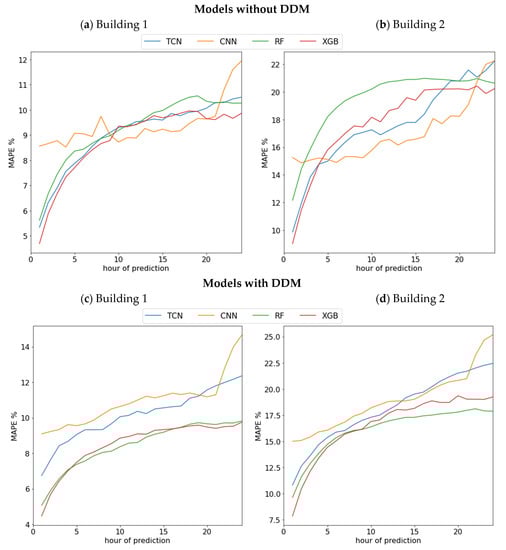
Figure 5.
(a) Performance of forecasting algorithms without DDM by hours in Building 1. (b) Performance of forecasting algorithms without DDM by hours in Building 2. (c) Performance of forecasting algorithms with DDM by hours in Building 1. (d) Performance of forecasting algorithms with DDM by hours in Building 2.
The results show that the proposed method can be applied to maintain or even improve the performance of learning algorithms in situations where there are constant changes in the behavior of electrical consumption in buildings. A limitation is the drift detection methods that were integrated. In the case of ADWIN, only the confidence value parameter was allowed to be modified, while in the case of KSWIN an inappropriate modification of the values of the size of windows would cause the method to not detect sudden changes in the distribution data.
5. Conclusions
In this paper, the integration of drift detection methods is analyzed in models for electricity consumption forecasting in buildings so that these models can adapt to the changing behavior that has been occurring in buildings due to energy-saving measures. Two active methods and one passive method were proposed to be integrated with the decision tree and deep learning models to know when the models should be retrained according to changes in the data distribution. The passive method consisted of retraining the models every 24 h assuming that the models should be constantly updated, while the active methods were ADWIN and KSWIN, which are based on a variable-length window approach.
The main conclusion that can be learned from this study, after analyzing the results, is that in the case of decision tree models, the incorporation of DDM not only allows them to keep up to date with changes in the data distribution but also improves their accuracy. Being the best case RF, without DDM obtained a MAPE of 9.23% for Building 1 and 19.47% for Building 2 while with the passive DDM it obtained a MAPE of 8.46% for building 1 and 16.14% for Building 2. However, in the case of deep learning models, the incorporation of DDM did not turn out to be as favorable as decision tree models. With the CNN being the worst case, without DDM an MAPE of 9.40% was obtained for Building 1 and 16.97% for Building 2 while with the passive DDM it obtained an MAPE of 10.93% for building 1 and 18.89% for Building 2. We can deduce from this that in the case of deep learning models, constantly updating them with small volumes of data would only worsen their performance. In cases such as Building 2 with sudden changes in load curves due to improvements, the model becomes inefficient, because deep learning models cannot adapt with small data to constant changes in the short term.
Considering the results obtained in the deep learning models, for future lines of research it would be necessary to focus on how it would be possible to adapt the deep learning models to constant changes within the electrical consumption forecasting in buildings to avoid model obsolescence.
Author Contributions
Conceptualization, D.M.-H., M.S. and L.H.-C.; methodology, D.M.-H. and L.H.-C.; software, D.M.-H., M.S. and V.A.-G.; validation, A.Z.-L., O.D.-P., L.G.-M. and F.S.G.; data analysis, D.M.-H., M.S., V.A.-G. and H.J.B.; investigation, D.M.-H.; data curation, D.M.-H. and M.S.; writing—original draft preparation, D.M.-H.; writing—review and editing, A.Z.-L., O.D.-P., A.O.-C. and A.J.-D.; visualization, D.M.-H. and M.S.; supervision, L.H.-C. All authors have read and agreed to the published version of the manuscript.
Funding
This research received no external funding.
Institutional Review Board Statement
Not applicable.
Informed Consent Statement
Not applicable.
Data Availability Statement
Not applicable.
Acknowledgments
The authors acknowledge the University of Valladolid and the Instituto Tecnológico de Santo Domingo for their support in this research, which is the result of a co-supervised doctoral thesis.
Conflicts of Interest
The authors declare no conflict of interest.
References
- IEA Tracking Buildings. 2021. Available online: https://www.iea.org/reports/tracking-buildings-2021 (accessed on 16 March 2022).
- Cholewa, T.; Siuta-Olcha, A.; Smolarz, A.; Muryjas, P.; Wolszczak, P.; Guz, Ł.; Bocian, M.; Balaras, C.A. An easy and widely applicable forecast control for heating systems in existing and new buildings: First field experiences. J. Clean. Prod. 2022, 352, 131605. [Google Scholar] [CrossRef]
- Devagiri, V.M.; Boeva, V.; Abghari, S.; Basiri, F.; Lavesson, N. Multi-view data analysis techniques for monitoring smart building systems. Sensors 2021, 21, 6775. [Google Scholar] [CrossRef] [PubMed]
- Izidio, D.M.; de Mattos Neto, P.S.; Barbosa, L.; de Oliveira, J.F.; Marinho, M.H.D.N.; Rissi, G.F. Evolutionary hybrid system for energy consumption forecasting for smart meters. Energies 2021, 14, 1794. [Google Scholar] [CrossRef]
- Hong, T.; Wang, Z.; Luo, X.; Zhang, W. State-of-the-art on research and applications of machine learning in the building life cycle. Energy Build. 2020, 212, 109831. [Google Scholar] [CrossRef] [Green Version]
- Kim, J.Y.; Cho, S.B. Electric energy consumption prediction by deep learning with state explainable autoencoder. Energies 2019, 12, 739. [Google Scholar] [CrossRef] [Green Version]
- Zeng, A.; Ho, H.; Yu, Y. Prediction of building electricity usage using Gaussian Process Regression. J. Build. Eng. 2020, 28, 101054. [Google Scholar] [CrossRef]
- Xu, W.; Peng, H.; Zeng, X.; Zhou, F.; Tian, X.; Peng, X. A hybrid modelling method for time series forecasting based on a linear regression model and deep learning. Appl. Intell. 2019, 49, 3002–3015. [Google Scholar] [CrossRef]
- Cholewa, T.; Siuta-Olcha, A.; Smolarz, A.; Muryjas, P.; Wolszczak, P.; Anasiewicz, R.; Balaras, C.A. A simple building energy model in form of an equivalent outdoor temperature. Energy Build. 2021, 236, 110766. [Google Scholar] [CrossRef]
- Žliobaitė, I.; Pechenizkiy, M.; Gama, J. An Overview of Concept Drift Applications BT—Big Data Analysis: New Algorithms for a New Society; Japkowicz, N., Stefanowski, J., Eds.; Springer International Publishing: Cham, Switzerland, 2016; pp. 91–114. ISBN 978-3-319-26989-4. [Google Scholar]
- Iwashita, A.S.; Papa, J.P. An Overview on Concept Drift Learning. IEEE Access 2019, 7, 1532–1547. [Google Scholar] [CrossRef]
- Baier, L.; Kühl, N.; Satzger, G.; Hofmann, M.; Mohr, M. Handling concept drifts in regression problems—the error intersection approach. In WI2020 Zentrale Tracks; GITO Verlag: Berlin, Germany, 2020; pp. 210–224. [Google Scholar]
- Kahraman, A.; Kantardzic, M.; Kahraman, M.; Kotan, M. A data-driven multi-regime approach for predicting energy consumption. Energies 2021, 14, 6763. [Google Scholar] [CrossRef]
- Webb, G.I.; Lee, L.K.; Goethals, B.; Petitjean, F. Analyzing concept drift and shift from sample data. Data Min. Knowl. Discov. 2018, 32, 1179–1199. [Google Scholar] [CrossRef]
- Lu, J.; Liu, A.; Dong, F.; Gu, F.; Gama, J.; Zhang, G. Learning under Concept Drift: A Review. IEEE Trans. Knowl. Data Eng. 2019, 31, 2346–2363. [Google Scholar] [CrossRef] [Green Version]
- Brzezinski, D.; Stefanowski, J. Reacting to different types of concept drift: The accuracy updated ensemble algorithm. IEEE Trans. Neural Netw. Learn. Syst. 2014, 25, 81–94. [Google Scholar] [CrossRef] [Green Version]
- Wadewale, K.; Desai, S.; Tennant, M.; Stahl, F.; Rana, O.; Gomes, J.B.; Thakre, A.A.; Redes, E.M.; Padmalatha, E.; Rani, P.; et al. Survey on Method of Drift Detection and Classification for time varying data set. Comput. Biol. Med. 2016, 32, 1–7. [Google Scholar]
- Khezri, S.; Tanha, J.; Ahmadi, A.; Sharifi, A. A novel semi-supervised ensemble algorithm using a performance-based selection metric to non-stationary data streams. Neurocomputing 2021, 442, 125–145. [Google Scholar] [CrossRef]
- Fekri, M.N.; Patel, H.; Grolinger, K.; Sharma, V. Deep learning for load forecasting with smart meter data: Online Adaptive Recurrent Neural Network. Appl. Energy 2021, 282, 116177. [Google Scholar] [CrossRef]
- Jagait, R.K.; Fekri, M.N.; Grolinger, K.; Mir, S. Load Forecasting Under Concept Drift: Online Ensemble Learning With Recurrent Neural Network and ARIMA. IEEE Access 2021, 9, 98992–99008. [Google Scholar] [CrossRef]
- Fenza, G.; Gallo, M.; Loia, V. Drift-aware methodology for anomaly detection in smart grid. IEEE Access 2019, 7, 9645–9657. [Google Scholar] [CrossRef]
- Mehmood, H.; Kostakos, P.; Cortes, M.; Anagnostopoulos, T.; Pirttikangas, S.; Gilman, E. Concept drift adaptation techniques in distributed environment for real-world data streams. Smart Cities 2021, 4, 349–371. [Google Scholar] [CrossRef]
- Ceci, M.; Corizzo, R.; Japkowicz, N.; Mignone, P.; Pio, G. ECHAD: Embedding-Based Change Detection from Multivariate Time Series in Smart Grids. IEEE Access 2020, 8, 156053–156066. [Google Scholar] [CrossRef]
- Yang, Z.; Al-Dahidi, S.; Baraldi, P.; Zio, E.; Montelatici, L. A Novel Concept Drift Detection Method for Incremental Learning in Nonstationary Environments. IEEE Trans. Neural Netw. Learn. Syst. 2020, 31, 309–320. [Google Scholar] [CrossRef] [PubMed]
- Silva, R.P.; Zarpelão, B.B.; Cano, A.; Barbon Junior, S. Time series segmentation based on stationarity analysis to improve new samples prediction. Sensors 2021, 21, 7333. [Google Scholar] [CrossRef] [PubMed]
- Heusinger, M.; Raab, C.; Schleif, F.M. Passive concept drift handling via variations of learning vector quantization. Neural Comput. Appl. 2022, 34, 89–100. [Google Scholar] [CrossRef]
- Raab, C.; Heusinger, M.; Schleif, F.M. Reactive Soft Prototype Computing for Concept Drift Streams. Neurocomputing 2020, 416, 340–351. [Google Scholar] [CrossRef]
- Togbe, M.U.; Chabchoub, Y.; Boly, A.; Barry, M.; Chiky, R.; Bahri, M. Anomalies detection using isolation in concept-drifting data streams. Computers 2021, 10, 13. [Google Scholar] [CrossRef]
- Moon, J.; Park, S.; Rho, S.; Hwang, E. A comparative analysis of artificial neural network architectures for building energy consumption forecasting. Int. J. Distrib. Sens. Netw. 2019, 15, 155014771987761. [Google Scholar] [CrossRef] [Green Version]
- Kiprijanovska, I.; Stankoski, S.; Ilievski, I.; Jovanovski, S.; Gams, M.; Gjoreski, H. HousEEC: Day-Ahead Household Electrical Energy Consumption Forecasting Using Deep Learning. Energies 2020, 13, 2672. [Google Scholar] [CrossRef]
- Zor, K.; Çelik, Ö.; Timur, O.; Teke, A. Short-term building electrical energy consumption forecasting by employing gene expression programming and GMDH networks. Energies 2020, 13, 1102. [Google Scholar] [CrossRef] [Green Version]
- Li, Z.; Friedrich, D.; Harrison, G.P. Demand Forecasting for a Mixed-Use Building Using Agent-Schedule Information with a Data-Driven Model. Energies 2020, 13, 780. [Google Scholar] [CrossRef] [Green Version]
- Culaba, A.B.; Del Rosario, A.J.R.; Ubando, A.T.; Chang, J.-S. Machine learning-based energy consumption clustering and forecasting for mixed-use buildings. Int. J. Energy Res. 2020, 44, 9659–9673. [Google Scholar] [CrossRef]
- Wang, Z.; Wang, Y.; Zeng, R.; Srinivasan, R.S.; Ahrentzen, S. Random Forest based hourly building energy prediction. Energy Build. 2018, 171, 11–25. [Google Scholar] [CrossRef]
- Sauer, J.; Mariani, V.C.; dos Santos Coelho, L.; Ribeiro, M.H.D.M.; Rampazzo, M. Extreme gradient boosting model based on improved Jaya optimizer applied to forecasting energy consumption in residential buildings. Evol. Syst. 2021, 1–12. [Google Scholar] [CrossRef]
- Bassi, A.; Shenoy, A.; Sharma, A.; Sigurdson, H.; Glossop, C.; Chan, J.H. Building energy consumption forecasting: A comparison of gradient boosting models. In Proceedings of the 12th International Conference on Advances in Information Technology, Bangkok, Thailand, 29 June–1 July 2021. [Google Scholar] [CrossRef]
- Mariano-Hernández, D.; Hernández-Callejo, L.; Solís, M.; Zorita-Lamadrid, A.; Duque-Perez, O.; Gonzalez-Morales, L.; Santos-García, F. A Data-Driven Forecasting Strategy to Predict Continuous Hourly Energy Demand in Smart Buildings. Appl. Sci. 2021, 11, 7886. [Google Scholar] [CrossRef]
- Olu-Ajayi, R.; Alaka, H.; Sulaimon, I.; Sunmola, F.; Ajayi, S. Building energy consumption prediction for residential buildings using deep learning and other machine learning techniques. J. Build. Eng. 2022, 45, 103406. [Google Scholar] [CrossRef]
- Lemos, V.H.B.; Almeida, J.D.S.; Paiva, A.C.; Junior, G.B.; Silva, A.C.; Neto, S.M.B.; Lima, A.C.M.; Cipriano, C.L.S.; Fernandes, E.C.; Silva, M.I.A. Temporal convolutional network applied for forecasting individual monthly electric energy consumption. In Proceedings of the 2020 IEEE International Conference on Systems, Man, and Cybernetics (SMC), Toronto, ON, Canada, 11–14 October 2020; pp. 2002–2007. [Google Scholar]
- Bendaoud, N.M.M.; Farah, N. Using deep learning for short-term load forecasting. Neural Comput. Appl. 2020, 32, 15029–15041. [Google Scholar] [CrossRef]
- Gao, Y.; Ruan, Y.; Fang, C.; Yin, S. Deep learning and transfer learning models of energy consumption forecasting for a building with poor information data. Energy Build. 2020, 223, 110156. [Google Scholar] [CrossRef]
- Bifet, A.; Gavaldà, R. Learning from time-changing data with adaptive windowing. In Proceedings of the 7th SIAM International Conference on Data Mining, Minneapolis, MN, USA, 26–28 April 2007; pp. 443–448. [Google Scholar]
- Moon, J.; Kim, Y.; Son, M.; Hwang, E. Hybrid Short-Term Load Forecasting Scheme Using Random Forest and Multilayer Perceptron. Energies 2018, 11, 3283. [Google Scholar] [CrossRef] [Green Version]
- Khosravani, H.; Castilla, M.; Berenguel, M.; Ruano, A.; Ferreira, P. A Comparison of Energy Consumption Prediction Models Based on Neural Networks of a Bioclimatic Building. Energies 2016, 9, 57. [Google Scholar] [CrossRef] [Green Version]
- Ali, U.; Shamsi, M.H.; Bohacek, M.; Hoare, C.; Purcell, K.; Mangina, E.; O’Donnell, J. A data-driven approach to optimize urban scale energy retrofit decisions for residential buildings. Appl. Energy 2020, 267, 114861. [Google Scholar] [CrossRef]
- Anđelković, A.S.; Bajatović, D. Integration of weather forecast and artificial intelligence for a short-term city-scale natural gas consumption prediction. J. Clean. Prod. 2020, 266, 122096. [Google Scholar] [CrossRef]


Publisher’s Note: MDPI stays neutral with regard to jurisdictional claims in published maps and institutional affiliations. |
© 2022 by the authors. Licensee MDPI, Basel, Switzerland. This article is an open access article distributed under the terms and conditions of the Creative Commons Attribution (CC BY) license (https://creativecommons.org/licenses/by/4.0/).