
Robust Optimization Model for Single Line Dynamic Bus Dispatching


Abstract
:1. Introduction
2. Literature Review
3. Robust Optimization Model
3.1. Basic Form
3.2. The Three Scenarios Considered
3.3. Assumptions
- The buses on the route during the planning horizon are the same type;
- Operating buses maintain the same order, and passing (overtaking) is not permitted;
- No accidents occur during the planning period, and vehicle operations and road conditions remain normal;
- The buses between stations operate at a constant speed that is set in advance;
- In the three scenarios of the planning horizon, the benchmark passenger flow data are obtained from real-time data and a forecasting algorithm. The respective and low passenger flow data are obtained by setting a certain offset on the base passenger flow data. Functions of passenger flow over time for each station can be obtained in the three scenarios;
- A bus stop exists at every station on the route without a cross-station phenomenon;
- The passenger bus boarding time and exiting time are the same;
- The passenger exiting rate at each station is constant during the same planning cycle.;
- Only the modeling process of the benchmark passenger flow is described; the other two scenarios are exactly the same, except for the passenger flow.
3.4. Objective Function
3.5. Constraint Condition
3.6. Model Summary
4. Solving Algorithms
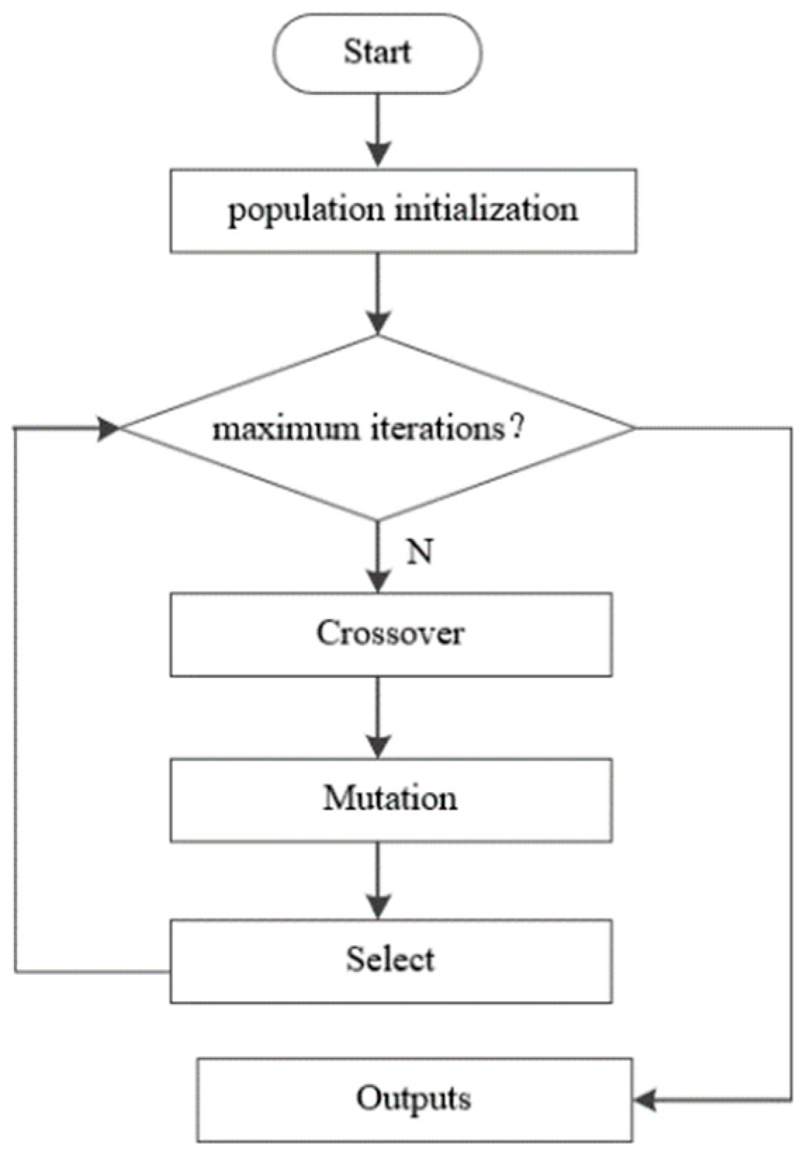
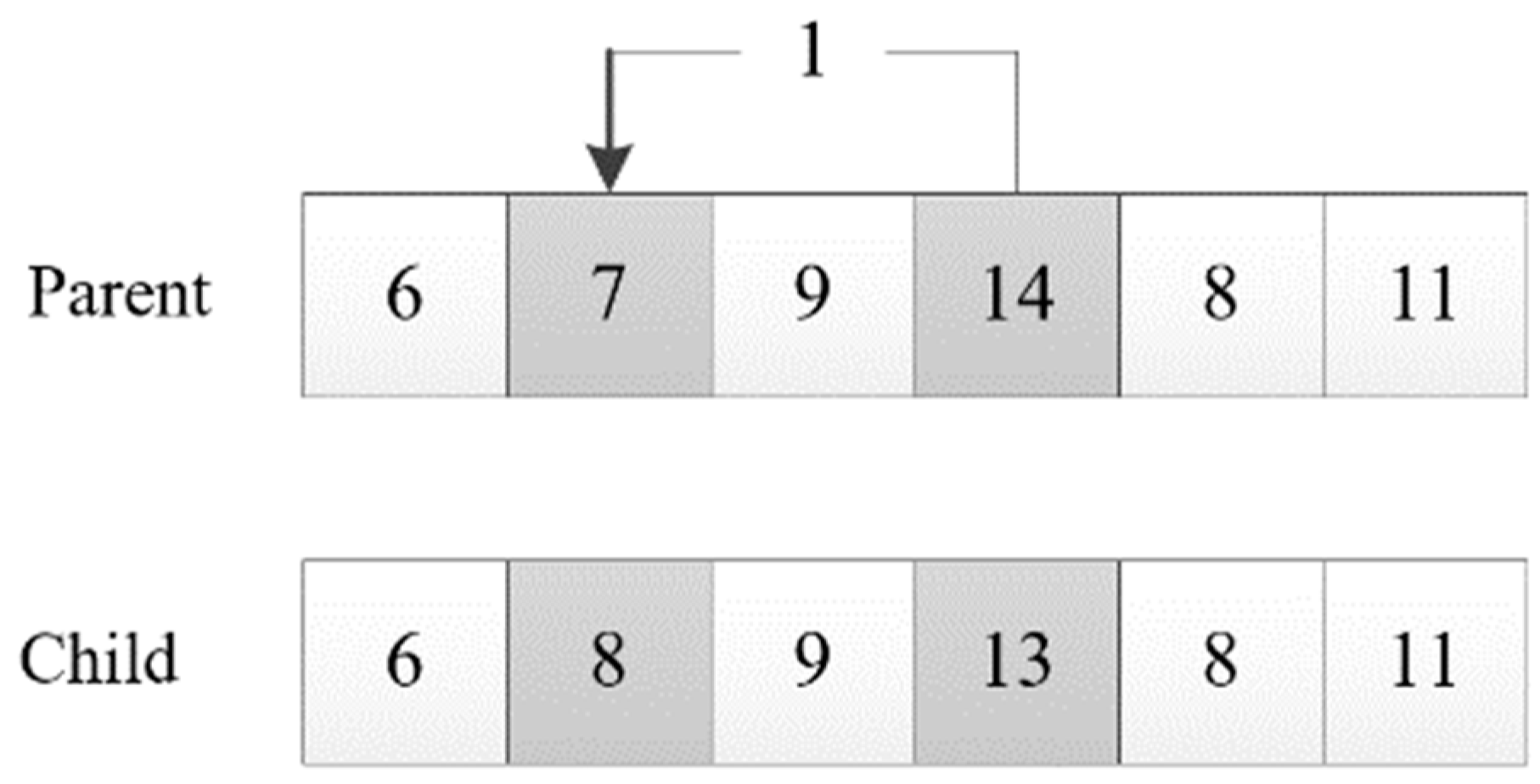
4.1. Genetic Algorithm
4.2. Improved Genetic Algorithm
5. Case Analysis
Experiments for a Single Bus Line
6. Conclusions
- (1)
- It starts with the definition of robust optimization when solving the model, and produces the optimal value in the worst case. In the future, more accurate and efficient methods can be considered, such as the tangent plane method and cone programming;
- (2)
- Considering the complexity of the model solution, the set scenario is relatively simple. In the future, the number of scenarios and detailed information can be considered to be more sufficient, so as to ensure that the complexity of solving the model is acceptable and the model is easy to solve;
- (3)
- The model and the case study are only for a single bus line; however, multiple bus lines may work simultaneously, and passengers may transfer from one line to another. In future research, the optimization model and algorithms can be extended for a multi-line scenario by considering the passengers’ transfers, and by coordination of departure times from different lines.
Author Contributions
Funding
Institutional Review Board Statement
Informed Consent Statement
Data Availability Statement
Acknowledgments
Conflicts of Interest
Nomenclature
| Parameters that are given for the whole planning horizon. | |
| i | the vehicle number, i = 1, 2,..., M + N |
| j | the station number, j = 1, 2,..., J |
| σ | the buffer time that a bus needs when it stops at a station with acceleration and deceleration |
| Cmax | the maximum capacity of a bus |
| α | the average time per passenger boarding and exiting (second/person) |
| qj | the ratio of passengers exiting when the bus arrives at station j (between 0 and 1) |
| DSj | the distance between station j − 1 and j (meters), j = 2, 3,..., J |
| Vj | the bus speed between station j − 1 and j, j = 2, 3,..., J − 1 |
| the stopping time of bus i at station j, i = 1, 2,..., M + N; j = 2, 3,..., J − 1 | |
| the time when bus i leaves station j, i = 1, 2,..., M + N; j = 1, 2,..., J − 1 | |
| the number of passengers waiting for bus i at station j when it arrives at station j, i = 1, 2,..., M + N;j = 1, 2, ..., J − 1 | |
| the number of passengers boarding bus i at station j after it arrives, i = 1, 2, ..., M + N; j = 1, 2, ..., J − 1 | |
| the number of waiting passengers who failed to board bus i at station j after it arrived, i = 1, 2,..., M + P; j = 1, 2,..., J − 1 | |
| the number of passengers exiting bus i at station j, i = 1, 2, …, M + N; j = 2, 3, …, J | |
| the number of passengers on bus i arriving at station j, i = 1, 2,..., M + P; j = 2, 3, ..., J | |
| Tavg | the expected wait time for passengers left behind by the last bus (unit of passengers) |
| Hma | the maximum departure interval |
| Hmin | the minimum departure interval |
| Parameters that can be predicted based on real-time data. | |
| λj = fj(t) | the passenger arrival rate function of station j, j = 1, 2,..., J − 1 |
| Parameters that are collected before the planning horizon starts. | |
| Pi | the number of passengers waiting for a bus at station j, j = 1, 2,..., J − 1 |
| Li | the sequence number of the upstream station that bus i is traveling on the route just passed, i = M + 1, M + 2, ..., M + N |
| Di | the distance between bus i traveling on the route and the upstream station that bus i just passed, i = M + 1, M + 2,..., M + N |
| the time when bus i is traveling on the route departed station j, i = M + 1, M + 2, ..., M + N; j = 1, 2,..., Li | |
| the number of passengers boarding bus i when it arrives at station j, i = M + 1, M + 2,..., M + N; j = 1, 2, ..., Li | |
| the number of passengers exiting bus i when it arrives at station j, i = M + 1, M + 2, ..., M + N; j = 1, 2, ..., Li | |
| Decision variable | |
| the departure time at the first stop of bus i, i = 1, 2,..., M; | |
References
- Song, D. Research on Regional Bus Timetable Scheduling Optimization; Huazhong University of Science and Technology: Wuhan, China, 2013. [Google Scholar]
- Ceder, A. Urban transit scheduling: Framework, review and examples. J. Urban Plan. Dev. 2002, 128, 225–244. [Google Scholar] [CrossRef]
- Ying, Z.; Jianhua, H.; Zhenmin, T. Research on dynamic bus scheduling model. Pract. Underst. Math. 2003, 33, 23–25. [Google Scholar]
- Luo, X.; Liu, Y.X.; Yu, Y.; Tang, J.F.; Li, W. Dynamic bus dispatching using multiple types of real-time information. Transp. B 2019, 7, 519–545. [Google Scholar] [CrossRef]
- Tian, J. Optimization Model and Algorithm of Supply Chain Management under Uncertain Conditions; Southwest Jiaotong University: Chengdu, China, 2005. [Google Scholar]
- Song, R.; Wei, H.; Yang, Y. Integrated optimization model of transit scheduling plan and bus use. China J. Highw. Transp. 2006, 19, 70–76. [Google Scholar] [CrossRef]
- Yan, S.Y.; Chi, C.J.; Tang, C.H. Inter-city bus routing and timetable setting under stochastic demands. Transp. Res. Part A Policy Pract. 2006, 40, 572–586. [Google Scholar] [CrossRef]
- Liu, X.; Wei, H.S. Study on bus dispatching model based on dependent-chance goal programming. Commun. Stand. 2006, 160, 152–155. [Google Scholar]
- Yu, C.S.; Daoud, H.; Li, L. Robust optimization model for stochastic logistic problems. Int. J. Prod. Econ. 2000, 64, 385–397. [Google Scholar] [CrossRef]
- List, G.F.; Wood, B.; Nozick, L.K. Robust optimization for fleet planning under uncertainty. Transp. Res. Part E Logist. Transp. Rev. 2003, 39, 209–227. [Google Scholar] [CrossRef]
- Goerigk, M.; Grün, B. A robust bus evacuation model with delayed scenario information. OR Spectr. 2014, 36, 923–948. [Google Scholar] [CrossRef]
- Goerigk, M.; Deghdak, K.; T’Kindt, V. A two-stage robustness approach to evacuation planning with buses. Transp. Res. Part B: Methodol. 2015, 78, 66–82. [Google Scholar] [CrossRef] [Green Version]
- Wei, W.; Liu, F.; Mei, S. Distributionally robust co-optimization of energy and reserve dispatch. IEEE Trans. Sustain. Energy 2017, 7, 289–300. [Google Scholar] [CrossRef]
- Gkiotsalitis, K.; Alesiani, F. Robust timetable optimization for bus lines subject to resource and regulatory constraints. Transp. Res. Part E Logist. Transp. Rev. 2019, 128, 30–51. [Google Scholar] [CrossRef]
- Liu, H.; Yang, C.; Yang, J. Robust transportation network design modeling with regret value. J. Transp. Syst. Eng. Inf. Technol. 2013, 5, 86–92. [Google Scholar] [CrossRef]
- Ma, C.; Wei, H.; Pan, F.; Wang, X.; Hu, X. Road screening and distribution route multi-objective robust optimization for hazardous materials based on neural network and genetic algorithm. PLoS ONE 2018, 13, e0198931. [Google Scholar] [CrossRef] [PubMed]
- Zhao, F.; Sun, H.; Zhao, F.; Zhang, H.; Li, T. A globalized robust optimization approach of dynamic network design problem with demand uncertainty. IEEE Access 2019, 7, 115734–115748. [Google Scholar] [CrossRef]
- Zhuang, G. Robust Optimization Model Research on Liner Fleet Deployment under Demand Uncertainty; Dalian Maritime University: Dalian, China, 2013. [Google Scholar]
- Bao, H. Robust Optimization of Liner Shipping Network of the Yangtze River Considering Fanba and Weather Influences; Dalian Maritime University: Dalian, China, 2014. [Google Scholar]
- Zhang, E.; Chu, F.; Wang, S.; Liu, M.; Sui, Y. Approximation approach for robust vessel fleet deployment problem with ambiguous demands. J. Comb. Optim. 2020, 5. [Google Scholar] [CrossRef]
- Lu, C.C.; Yan, S.; Li, H.C.; Diabat, A.; Wang, H.T. Optimal fleet deployment for electric vehicle sharing systems with the consideration of demand uncertainty. Comput. Oper. Res. 2021, 135, 105437. [Google Scholar] [CrossRef]
- Zhu, X.; Mengi, X.; Lei, M. Robust design and optimization of Urban Rail Transit Operation Scheme. Mod. Urban Rail Transit 2016, 1, 76–78, 82. [Google Scholar]
- Sels, P.; Dewilde, T.; Cattrysse, D. Reducing the passenger travel time in practice by the automated construction of a robust railway timetable. Transp. Res. Part B 2016, 84, 124–156. [Google Scholar] [CrossRef]
- Cao, Z.; Yuan, Z.; Li, D. Robust optimization model for train working diagram of urban rail transit. China Railw. Sci. 2017, 38, 130–136. [Google Scholar] [CrossRef]
- Wang, X.; Wang, S. Robust optimization of the coordinated passenger inflow control in a metro line under uncertain passenger demand. Shandong Sci. 2019, 12, 69–78. [Google Scholar]
- Qu, Y.; Wang, H.; Wu, J.; Yang, X.; Zhou, L. Robust optimization of train timetable and energy efficiency in urban rail transit: A two-stage approach. Comput. Ind. Eng. 2020, 146, 106594. [Google Scholar] [CrossRef]
- Soyster, A.L. Convex programming with set inclusive constraints and applications to inexact linear programming. Oper. Res. 1973, 21, 1154–1157. [Google Scholar] [CrossRef] [Green Version]
- Mulvey, J.M.; Zenios, S.A. Robust optimization of large-scale systems. Oper. Res. 1995, 43, 264–281. [Google Scholar] [CrossRef] [Green Version]
- Ben-Tal, A.; Nemirovski, A. Robust convex optimization. Math. Oper. Res. 1998, 23, 769–805. [Google Scholar] [CrossRef] [Green Version]
- Ben-Tal, A.; Nemirovski, A. Robust solutions to uncertain programs. Oper. Res. Lett. 1999, 25, 1–13. [Google Scholar] [CrossRef] [Green Version]
- Ben-Tal, A.; Nemirovski, A. Robust solutions of linear programming problems contaminated with uncertain data. Math. Program. 2000, 88, 411–424. [Google Scholar] [CrossRef] [Green Version]
- Bertsimas, D.; Sim, M. Price of Robustness. Oper. Res. 2004, 52, 35–53. [Google Scholar] [CrossRef] [Green Version]
- Yan, S.; Tang, C.H. An Integrated framework for intercity bus scheduling under stochastic bus travel times. Transp. Sci. 2008, 42, 318–335. [Google Scholar]
- Zhang, Y.; Tang, J. Risk-pooling-based robust model for least-time itinerary planning. J. Transp. Syst. Eng. Inf. Technol. 2014, 4, 107–112. [Google Scholar]
- Zhang, W.; Xu, W.A. Simulation-based robust optimization for the schedule of single-direction bus transit route: The design of experiment. Transp. Res. Part E Log. Transp. Rev. 2017, 106, 203–230. [Google Scholar] [CrossRef]
- Meng, J.M.; Liu, N.N.; Shi, H.F. Optimization of bus real-time arrival information based on robust optimization. J. Highw. Transp. Res. Dev. 2019, 9, 103–109. [Google Scholar]
- Ma, W.; Lin, N.; Chen, X.; Zhang, W. A robust optimization approach to public transit mobile real-time information. Promet Traffic Transp. 2018, 30, 501–512. [Google Scholar] [CrossRef]
- Wu, W.; Liu, R.; Jin, W.; Ma, C. Simulation-based robust optimization of limited-stop bus service with vehicle overtaking and dynamics: A response surface methodology. Transp. Res. Part E Log. Transp. Rev. 2019, 130, 61–81. [Google Scholar] [CrossRef]
- Pillac, V.; Gendreau, M.; Guéret, C.; Medaglia, L.A. A review of dynamic vehicle routing problems. Eur. J. Oper. Res. 2013, 225, 1–11. [Google Scholar] [CrossRef] [Green Version]


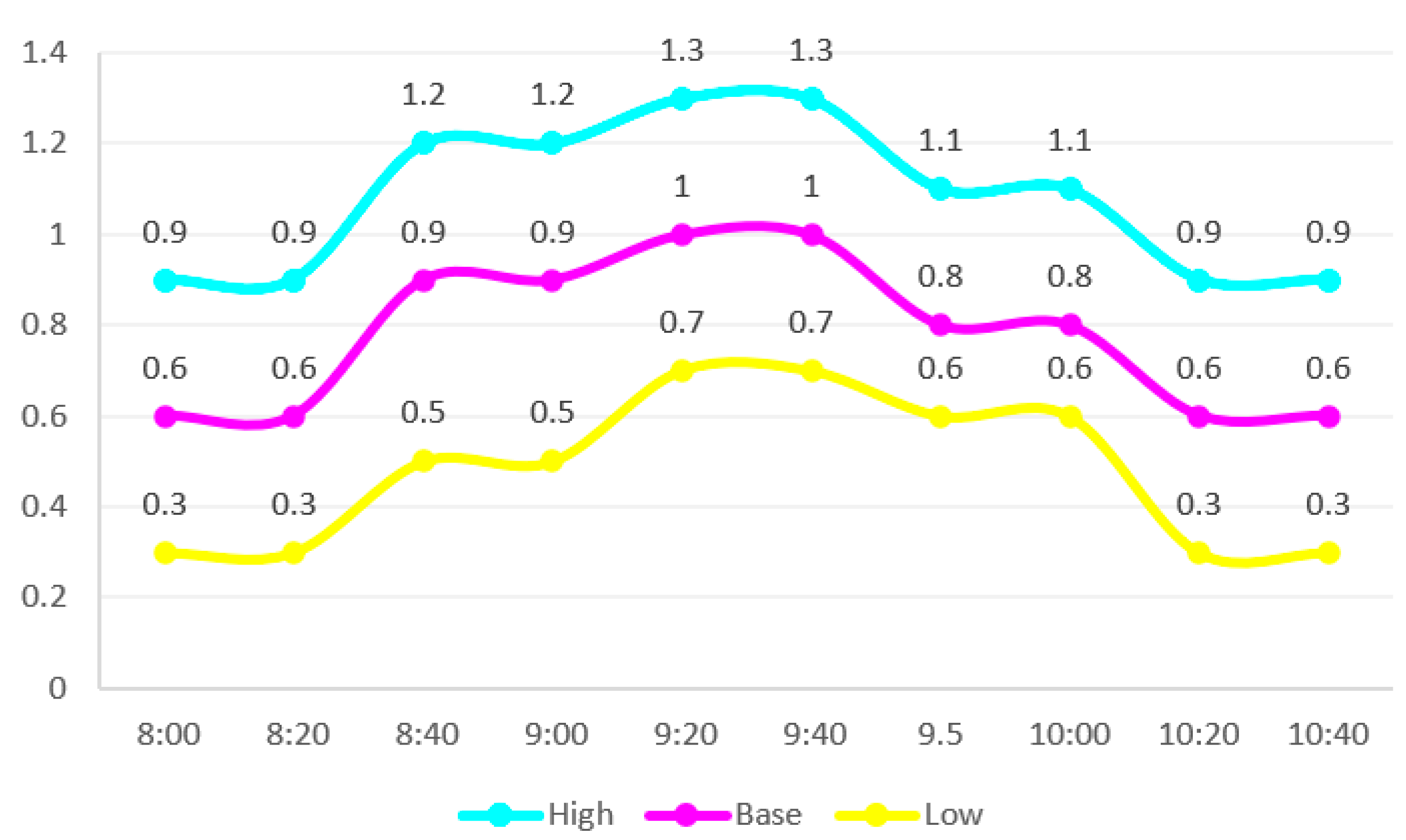
| Flow Scenario | Time | |||||||||
|---|---|---|---|---|---|---|---|---|---|---|
| 8:00 | 8:20 | 8:40 | 9:00 | 9:20 | 9:40 | 9.50 | 10:00 | 10:20 | 10:40 | |
| High | 0.9 | 0.9 | 1.2 | 1.2 | 1.3 | 1.3 | 1.1 | 1.1 | 0.9 | 0.9 |
| Base | 0.6 | 0.6 | 0.9 | 0.9 | 1.0 | 1.0 | 0.8 | 0.8 | 0.6 | 0.6 |
| Low | 0.3 | 0.3 | 0.5 | 0.5 | 0.7 | 0.7 | 0.6 | 0.6 | 0.3 | 0.3 |
| Results | Headway (Min) |
|---|---|
| Robust optimization results | 10 10 10 8 9 9 11 13 |
| Stochastic programming results | 10 10 10 8 9 8 10 15 |
| Scenarios | Optimal Solution Corresponding to the Total Waiting Time | Robust Optimization Solution Corresponding to Total Wait Time | Stochastic Optimization Solution Corresponding to Total Wait Time |
|---|---|---|---|
| Low passenger flow | 3184.99 | 3573.11 | 3831.44 |
| High passenger flow | 20,108.63 | 21,527.16 | 21,207.36 |
| Base passenger flow | 8406.08 | 8943.33 | 8907.29 |
| w | Total Waiting Time | Addition of the Total Waiting Time (%) | Reducing of the Maximum Regret (%) | |
|---|---|---|---|---|
| 1 | 0.23 | 11,582.14 | - | - |
| 2 | 0.20 | 11,585.81 | 0.03% | 13.0% |
| 3 | 0.17 | 11,585.81 | 0.03% | 26.1% |
| 4 | 0.13 | 11,644.43 | 0.32% | 43.4% |
| 5 | 0.10 | 11,668.62 | 1.04% | 56.5% |
| 6 | 0.07 | 11,733.16 | 1.15% | 69.6% |
| Zω* | Zω-ro | Zω-sp | Ws-d(%) | Wr-d(%) | |
|---|---|---|---|---|---|
| Low passenger flow | 3184.99 | 3452.29 | 3831.44 | 16.9% | 7.7% |
| High passenger flow | 20,108.63 | 21,652.20 | 21,207.36 | 5.2% | 7.1% |
| Base passenger flow | 8406.08 | 8965.01 | 8907.29 | 5.6% | 6.2% |
| Average value | 10,566.57 | 11,356.5 | 11,315.36 | - | - |
| Percentage increase | - | 7.0% | 6.6% | - | - |
| Standard deviation | - | - | - | 5.42% | 0.62% |
Publisher’s Note: MDPI stays neutral with regard to jurisdictional claims in published maps and institutional affiliations. |
© 2021 by the authors. Licensee MDPI, Basel, Switzerland. This article is an open access article distributed under the terms and conditions of the Creative Commons Attribution (CC BY) license (https://creativecommons.org/licenses/by/4.0/).
Share and Cite
Liu, Y.; Luo, X.; Wei, X.; Yu, Y.; Tang, J. Robust Optimization Model for Single Line Dynamic Bus Dispatching. Sustainability 2022, 14, 73. https://doi.org/10.3390/su14010073
Liu Y, Luo X, Wei X, Yu Y, Tang J. Robust Optimization Model for Single Line Dynamic Bus Dispatching. Sustainability. 2022; 14(1):73. https://doi.org/10.3390/su14010073
Chicago/Turabian StyleLiu, Yingxin, Xinggang Luo, Xu Wei, Yang Yu, and Jiafu Tang. 2022. "Robust Optimization Model for Single Line Dynamic Bus Dispatching" Sustainability 14, no. 1: 73. https://doi.org/10.3390/su14010073
APA StyleLiu, Y., Luo, X., Wei, X., Yu, Y., & Tang, J. (2022). Robust Optimization Model for Single Line Dynamic Bus Dispatching. Sustainability, 14(1), 73. https://doi.org/10.3390/su14010073