Abstract
MATSim is an open-source simulation framework for mesoscopic traffic simulations that has gained popularity in recent years. In this paper, we present a MATSim model for the city of Vienna, with a particular emphasis on the intermodal routing framework used to create agent trips, and the development of a utility function to specify different agents’ mode preferences. To create agent activity chains, we use mobility diaries from the national transportation survey in Austria and disaggregate the available geospatial information to best fit the reported travel times. The novelty of the intermodal framework is the ability to create trips that do not consist of only one mode of transportation, but to also include bicycle, car, and demand-responsive transport (e.g., cab, car sharing) trips in combination with public transportation. To represent the different mobility behaviors of agents, we divide the population into groups and assign them different utility functions for transportation modes according to their socio-demographic characteristics. After presenting the validation of the model, we discuss ways to improve the model.
1. Introduction
Agent-based simulations have been developed as a popular way of carrying out microscopic simulations. A leading simulation framework in the field of transportation research is MATSim [1]. In several publications, researchers describe different procedures for creating a MATSim model. One of the first models is the model for Zurich [2], while several other MATSim models have since been built (see [1], Chapter 52–97) that incorporate various specifications of local conditions related to data availability and specific transport modes.
In Bekhor et al. [3], the authors described their MATSim model for the Tel Aviv region for which they integrated travel demand generation (an activity-based model) with a dynamic modeling framework (MATSim framework). For the activity-based model, the authors used a hierarchy of logit and nested logit models to determine the purpose, time of day, destination, and mode of the main trip. These trips were then used as agent schedules for the MATSim simulation in which the routing of the trips took place. Another well-known example of creating a MATSim model is the open-source model for Berlin by Ziemke et al. [4]. The authors used the population generator CEMDAP (Comprehensive Econometric Microsimulator for Daily Activity-Travel Pattern) to generate daily activity and travel patterns for the agents. This activity generation was performed multiple times to create multiple schedules for each agent with different activity locations, times, and types. The MATSim framework with its CaDyTS (calibration of dynamic traffic simulations) [5] module was used sequentially to select trips that correspond to the traffic volumes of the counting stations. MATSim models are, at their simplest, based on census data (place of residence and place of work supplemented by additional points of interest) or rely on traffic surveys that already include trip chains to facilitate the search for secondary activity locations. Some models have also integrated various data sources that are increasingly available for some regions. These include, for example, georeferenced data from social media platforms, cell phone data, or smart card data for public transit [6]. The MATSim model for Dublin enriched the census and national travel survey with a destination choice model based on a radiation model. Georeferenced user data from Twitter and Foursquare were used to calibrate this radiation model. The population synthesis in the Singapore [7] model consisted of several models (e.g., population distribution, driver’s license model, car ownership model) and was further improved by Fourie et al. [8] using public transit smart card data.
Another line of research focuses on developing models based on publicly available data. This includes, for example, information on activity travel, as in the model for the city of Santiago de Chile. The city authority published aggregated data on travel behavior in the form of origin-destination matrices which Kickhofer et al. [9] used along with other openly available data to create a MATSim model for the region. Hörl and Balac [10] further elaborated in their work how to assemble a model from open and publicly available data in France. The authors prepared a workflow for building MATSim models in each French region. The raw data served as input for the “Population Pipeline”, an open-source generator of populations. This was then used as input for agent-based simulation programs such as MATSim or SUMO (Simulation of Urban MObility [11]). This approach has also been applied to other countries such as Sao Paolo [12].
In this paper, we present a MATSim model for Vienna and address the problems that many models face. One of them is that population synthesis does not guarantee plausible travel times for trips, since the model has been calibrated with census data. Such problems can be observed, for example, in the Amsterdam model [13]. Another problem we want to address is how to better represent the different mode choices of the agents. This issue of agent-specific preferences is identified as a research gap in Horni et al. [1], p. 540f.
The presented model has already been briefly described in Müller et al. [14]. There are two issues that we describe in more detail: The first is the integration of reported travel time of trips from the travel survey into the process of activity location selection. To do this, we present the routing framework Ariadne, which is used in performing the population synthesis and running the MATSim scenarios. The routing framework is able to compute routes consisting of a combination of different modes. The second objective of this work is to represent the different mode choice behavior of agents according to their socio-demographic characteristics. Usually, the distinctions in the utility functions of mode choice are based on the centrality of the agent’s residence. In Hülsmann [15], for example, agents living in the periphery have a higher tendency to use their cars. In this paper, we present a method that divides the population into several subpopulations based on a latent class model for which the parameters of the mode choice model have been estimated.
This article is structured as follows: Section 2 will explain the methods to build the model. After explaining the creation of the necessary input of the model (network, population, facilities), we introduce the generation of intermodal plans and describe the procedure of assigning different utility functions to groups of agents in the simulation to better distinguish heterogeneous mode choice behaviors. In Section 3, we describe the calibration and validation of our model. We conclude with the discussion of the results in Section 4.
2. Materials and Methods
2.1. Population Synthesis: Network, Facilities and Activity Chains
In order to represent the city traffic in Vienna in our model in an adequate way, the periphery outside of the city borders in the simulation is included. The area does not cover the whole agglomeration of Vienna but several commuter suburban areas within a 30 km radius from the city center as shown in Figure 1. The boundary of the simulation area is chosen in a way that includes important infrastructure (like bridges over the Danube river). Trips to and from locations outside of the simulation area are not included in the current version of the model.
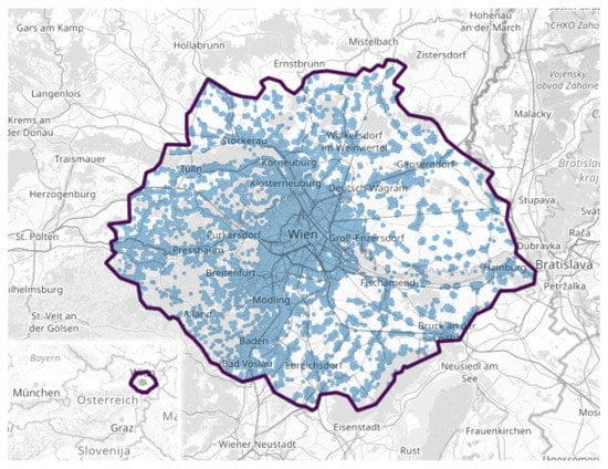
Figure 1.
Map of the simulation area. Blue dots indicate the location of facilities.
The population of the city of Vienna and of the simulated metropolitan area amounts to a total of 2.33 million people (2019) [16] with the simulation area covering 4170 km. The car routing graph for the simulation area is based on the OpenStreetMap (OSM) road network and consists of about 156,000 links and 71,000 nodes. The conversion of the network graph is done by using the pt2matsim framework. Time schedules for public transit (subway, trains, buses) are provided through GTFS (general transit feed specification) data sets provided by the transit operators.
MATSim requires the exact locations where activities of agents take place. The spatial information for these facilities are estimated by combining several geospatial data sets including land-use (OSM), points of interest (OSM), population density [17] and workforce [18].
Once the possible locations for performing an activity have been identified, they are used as the input for the generation of agent plans. The basis for the trip chains comes from the Austrian national mobility survey (“Österreich unterwegs 2013/2014” [19]) which provides daily travel-diaries that include each trip start and end along with the corresponding time, location (on municipal district level), purpose, and main mode of transportation used. The main mode is hereby determined by the hierarchy as defined in Fellendorf et al. [20]: PT > car > bike > walk. This means that a trip consisting of, for example, a car leg and a PT leg is categorized as a PT trip, regardless of how long the car leg was.
Due to observed misreporting of the travel distances, amendments based on travel times and detailed locations were derived by the survey authors. The resulting base data consists of 17,070 households and 38,220 persons each providing data on two sampling days and a total sample size of 196,604 trips. Each household is assigned a grossing-up factor to indicate the representativeness of the household within the sample relative to the total population.
Creating a simulation population requires several cleaning steps to fill in missing fields with derivable information; correct the coding of inconsistent time data; and remove records that are insufficient for this purpose. As a result, the cleaned data includes approximately 32,000 unique person-days as prototypical mobility patterns of persons over 6 years of age from 15,000 households which corresponds to persons in the national population. Restricting these samples to one working day in the study area yields 9900 unique person-days and describes the mobile population traveling in the model area of Greater Vienna. Additional data on households, such as household size, vehicle availability, self-assessment of economic situation, accessibility of public transport, and socio-economic data such as age, occupational status, highest level of education, or possession of season tickets for public transport are included in the national survey. The socio-economic characteristics are assigned to the synthesized agents, providing information that is later used to specify the mode choice behavior (see Section 2.3).
Activity locations are available at the municipal district level and these may be larger than the usual traffic analysis zones. Since districts in Vienna vary widely in size and can encompass large parts of the city, randomly selecting facilities from a district would, for an agent, result in widely varying trip suggestions. This would likely lead to the above mentioned issue of a mismatch between reported and simulated average trip distance and duration. Therefore, a spatial disaggregation algorithm is developed to select locations for agent activities such that the routed trip durations best fit the survey information. To obtain the necessary multi-modal trip durations, the optimization algorithm uses the Ariadne routing framework which is described in Section 2.2. It is computationally inefficient to provide a travel time for each mode and for each location of activity in the network. Therefore, the facilities are assigned to clusters with an edge length of approximately 500 m. For each cluster centroid, travel time to all other centroids is specified for each mode by Ariadne.
When drawing agents, the grossing-up factor is also taken into account, as this ensures the representativeness of the sample. As a result, reported trip diaries are used multiple times to generate agent plans in the simulation. For this reason, randomization of the facilities within the cluster is performed when drawing from the sample ensuring varied travel patterns for agents generated from the same survey prototype.
In our simulation model, 12.5% of the mobile population is represented over 6 years, which represents about 83% of the total population. Hence, we obtain in the simulation area a set of about agents performing trips in the simulation area and trips in the city of Vienna.
Running 100 iterations of the MATSim simulation on a server with an Intel Xeon CPU E5-2660 v3 @ 2.60 GHz processor and 30 GB RAM took about 12 h. For the baseline model, we ran 500 iterations in about 60 h, resulting in differences in modal split from one iteration to the next of less than for each mode (in percent).
2.2. Intermodal Routing
The default approach to the generation of varying departure times, activity locations or travel modes in MATSim, the so-called plan innovation, is strongly based on random mutations of an agent’s plan. The choice of transport mode works well for unimodal day plans (e.g., driving everywhere or solely using public transport (and walking) the whole day). The simulation converges to a stable optimum in an acceptable amount of time. However, when intermodal traffic is considered, the combinatorial options grow exponentially and so does the simulation time. In Hörl et al. [21] a mode choice framework is presented, which narrows down potential possible options to the most attractive ones from the agent’s perspective. The key concept is to look at the plausibility of the whole plan (i.e., all trips of an agent’s day) holistically and not at separate trips. Only plausible plans will be executed in the simulation.
MATSim supports intermodal routing through the Swiss rail raptor public transport router [22], which allows other modes than walking for access and egress to public transport. It respects mode availability (e.g., bike and car ownership) at the start of the agent’s day and keeps track of personal vehicles during the day so that a parked vehicle can only be retrieved at the place where it is parked. The process is based on the mode choice framework presented in Hörl et al. [21].
Ariadne as outlined by Prandtstetter et al. [23] is a closed source intermodal routing framework developed for research purposes at AIT Austrian Institute of Technology [24]. Route calculation supports individual traffic such as walking and cycling (respecting terrain) or driving as well as public transport and all possible intermodal combinations thereof. Free-floating and station-based sharing modes are supported as well.
We aim to build a completely intermodal MATSim model that does not restrict mode combinations to access and egress of public transport but instead enabling a bike sharing trip between two public transport trips. Our model combines Ariadne with the concept from Hörl et al. [21]. In short, Ariadne is used to calculate a few realistic intermodal plans (for the agent’s day) and feeds them randomly into the simulation during the replanning phase in the MATSim loop (see Figure 2). The MATSim network only consists of car links while the detailed routes for other modes are calculated with a detailed intermodal graph by Ariadne. Mode availability and the location of the agent’s personal vehicles are taken into account. This means that the personal vehicles must be returned home at the end of the day and can only be used at a given location if the agent has previously driven there. Together with a caching mechanism for the intermodal routing process, this achieves a fully intermodal traffic simulation that converges towards a state of equilibrium quickly.
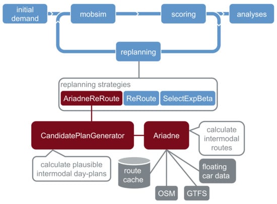
Figure 2.
Extension of the standard MATSim loop with intermodal plan generation.
2.2.1. Replanning Strategies
Ariadne is linked to the replanning stage of MATSim by providing the AriadneReRoute strategy. If this strategy is selected for replanning, the previous plan is replaced with a new plan calculated by the CandidatePlanGenerator. This strategy is intended to be used in combination with the strategies ReRoute and SelectExpBeta, which are part of MATSim core and recalculate routes for main modes and select plans, respectively (details in Horni et al. [1], pp. 39–41). The configuration is set in the way that the replanning strategies AriadneReRoute, ReRoute and SelectExpBeta are chosen with a probability of , , and , respectively. The weights chosen guarantee a sufficient balance between plan innovation and convergence of utilities.
2.2.2. CandidatePlanGenerator
The CandidatePlanGenerator calculates intermodal plans for the whole day based on the agents’ original plans. Before explaining the process in detail we first define the building blocks of an agent’s plan.
- activity an agent’s activity such as work, leisure, shopping
- trip route between two activities (can use one or more modes, e.g., walk + public transport + walk)
- trip type mode of transport or a combination thereof
- subtour two or more trips that form a loop, i.e., the start of the first trip is the end of the last trip
- home-subtour a subtour that starts and ends at a home location
- plan multiple trips (and activities in between) representing the whole day of an agent
Trip types vary from model to model but typically include:
- unimodal: walk, bike, car, public transport (PT)
- intermodal: bike and ride (B + R), park and ride (P + R)
For the model described in this work, the additional unimodal type demand responsive transport (DRT) (such as carsharing) and the intermodal type DRT and ride (D + R) can be added. In the described baseline mode in this article however, we will not consider DRT as it is not mentioned as a specific mode in the transport survey.
The basic principle of the CandidatePlanGenerator is to calculate routes for different (combinations of) modes of transport for all trips and then combine these trips into new plans. Simply generating all possible combinations of trips with all modes of transport would result in an unfeasible amount of plans that are also unrealistic (e.g., using a private car in the middle of the day when the agent did not leave the house by car in the morning). Therefore, we use the following algorithm to generate a limited number of plans that cover the most feasible mode combinations.
For each agent:
- The agent’s plan is split into home-subtours—for most plans there will only be one home-subtour. Note that these subtours are not necessarily loops because the locations for home activities may be different (e.g., one home location can be the agent’s flat, another home location the agent’s partner’s flat).
- For each home-subtour candidate plans are calculated.
- The candidate plans (of all home-subtours) are then combined per trip type to represent the whole day of the agent. The result is one candidate plan spanning the agent’s day for each trip type—except for trip types where one or more candidate plan are invalid (e.g., because cycling 200 km is not feasible)
For each home-subtour the candidate plans are calculated as follows:
- For each trip in the home-subtour alternative trips according to the defined trip types (i.e., mode combinations) are calculated.
- For unimodal trip types (and trip types containing DRT) the different trips are chained together. In case a trip is not available for a certain mode (e.g., a trip may be too long to be feasible for walking) a fallback mode can be used as follows:
- walk: combine walk trips, fallback to insert (replace with) PT if necessary
- bike: no fallback
- car: no fallback
- PT: combine PT trips, fallback to walk if necessary
- DRT: combine DRT trips, fallback to walk if necessary
- D + R: combine D + R trips, fallback to PT, DRT, walk if necessary
- For B + R and P + R (i.e., trip types with private vehicles in combination with public transport plans), we ensure that the private vehicle is used for at least the first and last trip so that the vehicle is returned home. In between, we combine PT trips and fall back to walk if necessary.
The availability of bikes and cars and driving license ownership are respected. It is assumed that the use of public transport, public transport and walking is possible for each agent. If a private vehicle (such as a bike) is available for an agent, it is assumed to be present at the first activity of the original plan, cannot be taken on public transport, and must be returned to the last activity of the plan.
For every plan, activity times of the original plan are adjusted. This is necessary to avoid bad scores for being to late as a consequence of a plan that was originally synthesized for a fast mode of transport but is unfeasible for a slower mode of transport. We argue that most activities, except for education and work, which remain fixed, are flexible. For home activities, start and end times as well as the duration can be changed. For errand, leisure, and shopping activities, the duration is preserved but they may be shifted in time. That means, for example, that agents switching to a slower mode of transport on their way to work leaves home earlier in order to avoid being late.
2.2.3. Route Cache
Without caching, the route calculations required for building candidate plans consume a (much too) high percentage of the MATSim run. Candidate plans are quickly created when needed during the simulation because routing requests to Ariadne are cached in an on-disk cache that is initialized once and can be used for multiple scenarios as long as the population does not change.
The key for a cached route consists of the location of the trip’s origin and destination, the modes of transport and the departure time. To maximize reuse of public transport routes, the departure times can be reduced to categories such as night, morning, noon, etc. The performance benefit weighs greater than the loss in precision for most projects.
Changing travel or waiting times due to evolution patterns in MATSim are considered even for cached routes: all segments using modes that are simulated on the network (i.e., not teleported) are re-routed using MATSim’s internal router.
2.3. Mode Choice Behavior
Agents in the simulation evaluate their activity durations and mode choices according to a utility (or scoring) function [1]. The parameters of this function are commonly estimated with a mode choice model. These mode choice models generally do not differentiate between different behaviors among the population groups. In our model, however, we try to incorporate different behaviors of the population in dependence of the socio-economic variables by applying a Latent Class Mode Choice Model (LCMCM). LCMCMs have been applied in Mode Choice Modeling regularly (see e.g., [25,26,27]). There are also first inclusions of latent class models in microscopic simulations for car following behavior in Koutsopoulos and Farah [28] but to our knowledge they are not applied to model group specific behavior in mesoscopic simulation models.
2.3.1. Parameter Estimation
The mode choice model taken for simulation is derived from the mobility, activity and expenditure diary data presented in Hössinger et al. [29] and is a simplified version of the model presented in Schmid et al. [30]. This data set contains a weekly mobility and activity diary and expenditure data from a representative sample in Austria. The study participants are also asked about their hypothetical transport mode choices (stated preferences). This detailed data set allows not only the estimation of the value of travel time saving (VTTS) and other mobility-related preference parameters, but also the estimation of the value of leisure (VoL). The VoL refers to the marginal (dis-)utility associated to the loss of time for leisure due to extended times spent on other activites. The VTTS and other travel-related preference parameters are derived from a LCMCM with two classes, applied to all trips included in the sample. For the Austrian data set, these estimations have been performed separately in Hössinger et al. [29] for the VoL and in Schmid et al. [30] for the VTTS. For our model, we refer to the joint estimated parameters as done by Jokubauskaitė et al. [31] which has the advantage that correlations between time use, expenditures and mode choice behavior can be accounted for in a coherent way. The parameters are slightly simplified to match the socio-economic characteristics used by the national transport survey data. Estimating VoL requires fitting observed expenditures and time use patterns to the utility maximization framework developed by Jara-Díaz et al. [32] using maximum likelihood estimation.
The LCMCM has two (latent) classes of coefficients for all parameters (see Figure 3). A higher number of classes turns out be unnecessary since there is no observable increase in the explanatory power. The latent classes are linked to the observable discrete variables via a common likelihood function and a common class membership equation [33]. This equation determines the class membership probability for each individual. The probability can be considered as the likelihood that an agent being part of the reference class and is a linear function based on binary socio-economic variables. The considered variables for our model are selected because of their availability in the estimated mode choice data and the synthesized population of agents. They are gender, age under 35, age over 55, income higher than the median, schooling higher than the median, living in an urban area, children in the household, single household, and working full-time at least 38 h per week. The exception is the variable high income for which self-reported standard of living was used as a proxy.
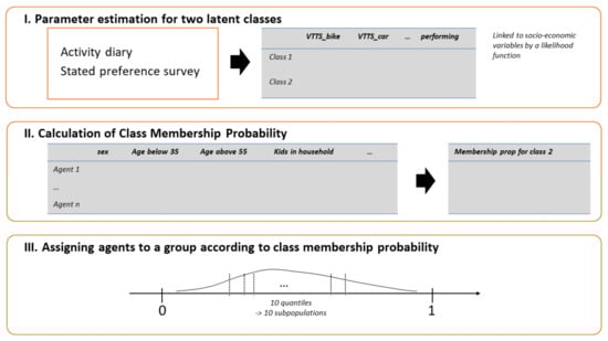
Figure 3.
Overview of the latent class model for the mode choice model and the derivation of subpopulations.
The quantiles of the class membership probabilities are used to split the populations into ten equally large subpopulations, with parameters calculated according to the average class membership probabilities. More specifically, the mode-specific constants, the VTTS, VoL, and the disutility associated with transferring public transport vary across subpopulations. The parameters are presented in Section 3.1, Table 1.

Table 1.
Parameters from the choice model to calculate the subpopulations’ parameters for the Charypar-Nagel function. refers to the not yet calibrated constants, to the value of travel time savings (VTTS), here noted as disutility, and indicates the value of leisure.
In addition, the parameters for lateArrival, waiting, and waitingPt are set different from the default. According to the meta-analysis of [34], the disutility for arriving 10 min late to an activity is on average times the disutility associated with a 10-min increase in in-vehicle time. Waiting for a facility to open is penalized by times the pt-in-vehicle time and waiting for public transportation is penalized by times the pt-in-vehicle time. Thus, consistent with the implementation in MATSim ([1], p. 29), the parameters are set as follows:
with and representing the VTTS for car and public transit and indicating the VoL.
2.3.2. Permanent Costs
The cost of owning and driving a car follows estimates from ADAC [35] for average vehicles. The fixed cost of a car is assumed to be EUR per day excluding an additional expenditure of EUR per kilometer driven. These costs are implemented by the parameters dailyMonetaryConstant and monetaryDistanceRate. Bicycle costs are estimated to be 1 EUR per day [36]. Public transportation travel costs for agents without a concession card or an annual ticket card are manually configured by taking the average of station-to-station fares. This results in a cost of EUR per day in Vienna ( EUR per day for trains) and EUR per day (and an additional EUR per kilometer) outside of Vienna. All financial expenditures are direct disutilities in the utility function in case the mode has been used at least once.
3. Results
3.1. Scoring Parameters
Based on the model described in Section 2.3, the parameters in Table 1 show the estimated VTTS for each mode () and the corresponding mode-specific constants (). The constant for walking is set to 0 for all subpopulations as reference parameter. The values are already normalized by the marginal utility of the mode choice model’s income, so that the marginalUtilityOfMoney is left at 1.
The VTTS is equal to VoL (i.e., the opportunity cost of time) minus the direct utility (or disutility) associated with time spent traveling (which typically depends on travel conditions such as crowding, comfort, and the ability to use travel time productively). The VoL, often referred to as in the MATSim literature, and is used directly as MATSim configuration parameters performing and utilityOfLineSwitch respectively. The performing parameter is rarely estimated in mode choice models. For this reason, the parameter is usually set to the VTTS of the car and all other modes are set relative to it ([1], p. 32). With an estimated VoL as in our case, however, we can define the marginalUtilityOfTraveling_util_hr parameter as the sum of and for all modes.
3.2. Calibration
The calibration of the model is carried out using count data on motorways and main roads, as well as adjusting the constants for the traffic modes in the utility function. In the calibration process we follow the approaches of Kickhofer et al. [9] and Ziemke et al. [37]. For each agent, multiple plans are provided, resulting from multiple sampling as described in Section 2.1. As recommended by Ziemke et al. [4], the number of initial plans is set to 4, and the maximum number of plans per agent is set to 8. Together with CaDyTs, calibration of the initial mode constants (see Table 1) is performed until the modal split per main mode matches the reported data [9]. To obtain the calibrated population, the constants were adjusted by −9 for bike, −2 for car, and −5.25 for PT. A differentiation of the adjustment according to subpopulations could not take place due to the lack of precise measurement data of the mode choice. Figure 4a presents the final modal split with an error of less than 1% per mode. Figure 4b shows how the modal splits differ in the subpopulations. In particular, for agents of subpopulations 9 and 10, who primarily live in non-urban areas, a reduced share of walk-trips and an increased share of car trips is evident. Intermodal trips are not specifically mentioned in the national transport survey, since they categorize trips by the main mode. In the simulation, around % of the agents’ trips are done with bike and PT, and % are done with car and PT. Though the share is quite low, the option of intermodal routing becomes important when new transportation modes (such as DRT shuttles) are introduced to the model.
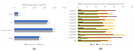
Figure 4.
(a) Modal split by main mode in the simulation (blue) and the report (grey). (b) Modal split by main mode for each subpopulation.
For the peak hours, we obtain a normalized mean relative error at counting stations in Vienna is 34.2% in the morning and 33.0% in the evening rush hour. The sum of the relative errors, is −5.9% in the morning and −14.2% in the evening.
Figure 5 shows a comparison between measured and simulated traffic volumes for a counting point close to the city center. The simulated night-time activities are underrepresented as they are often carried out at the end of an agent’s day in hours 24–30.
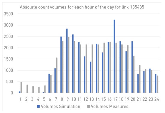
Figure 5.
Comparison between simulated and measured count volumes at Franz-Josefs-Kai near Schwedenplatz (outbound).
3.3. Validation
Validation of the simulation is also performed for traffic indicators other than those used for calibration. We compare the reported data from the national transport survey with the results from the simulation in terms of trip distance, trip duration, trip purpose and trip speeds.
3.3.1. Distance
Figure 6a shows the percentage distributions of the reported and simulated trip distances. The distributions are largely in line with each other, with deviations for very short and very long distances; mid-range distances of 1 to 2.5 km are overrepresented. The fact that short distances are underrepresented is assumed to come from the fact that start and end facility locations of a trip are not drawn from the same cluster. Therefore, very short trips of less than 500 m are not adequately included. The overall average distance in the simulation is 7.5 km, which is slightly lower than the reported distance of 8.3 km. An explanation for this observation is that surveyed outliers (e.g., those trips >50 km) can greatly distort the average of reported travel distances. Figure 6b shows the average trip distance per main mode which is simulated quite correctly for every mode except for car. The modal split per distances category, as presented in Figure A1 (in the Appendix A), shows a quite correct pattern for all modes. Just the walk trips in between 1–2.5 km are overrepresented in the simulation.
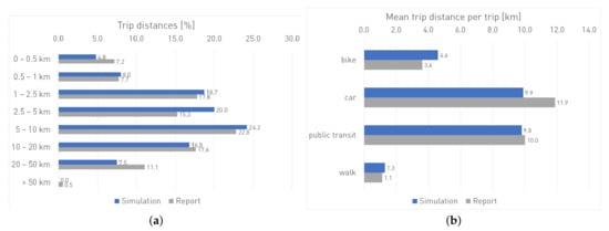
Figure 6.
(a) Distribution of trip distances and (b) mean trip distances by main mode in the simulation (blue) and the report (grey).
3.3.2. Duration
Further validation is possible by comparing the trip durations. The comparison between the reported and the simulated trip durations, as shown in Figure 7a, displays a similar pattern to the trip distances. Very short trips are clearly underrepresented in the simulation, while trips between 20 and 30 min are overrepresented. The reasons for this discrepancy are likely similar to the differences between the simulated and the reported trip distances. The mean trip duration of 28.5 min in the simulation is consistent with the reported trip duration of 27.8 min. Figure 7b shows that the simulated and reported trip durations show good consistence, where only simulated walking distances appear slightly too long.
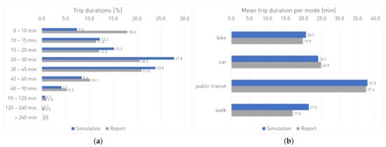
Figure 7.
(a) Distribution of trips’ duration and (b) mean trip durations by main mode in the simulation (blue) and the report (grey).
3.3.3. Purpose
The model proves to be very accurate for trip purposes. The distribution of trip purposes matches the reported values almost perfectly (Figure 8a). A comparison of the distribution of main modes by trip purpose in Figure 8b exhibits very good consistence for all purposes.
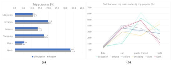
Figure 8.
(a) Distribution of trips’ purposes in the simulation (blue) and the report (grey). (b) Distribution of trip main modes by trip purposes. Reported values are marked as dashed lines.
Figure A2 (in the Appendix A) describes the distribution of distance category by trip purpose. Work trips and visits show only minor differences between the reported and simulated distributions. While leisure activities, education trips and errands are mostly consistent, an underestimation of the very short distances—and a resulting slight surplus of longer trips—is discernible. For shopping activities, this difference is more pronounced. Almost every fifth shopping trip is reported to be less than half a kilometer, while in simulations, these trips tend to be longer. The aforementioned restriction to draw trips within a cluster is the suspected cause of the inconsistency here.
3.3.4. Speed
Speeds for trips are examined by main mode and distance categories. Figure A3 shows that most similarities exist for the teleported modes of walk, bike, and public transit. For car, there are matches for longer distances above 10 km/h, while shorter distances are represented with a lower speed in the simulation. One reason for this may be the inadequately specified trip durations in the report by the survey participants, which are based only on roughly recorded start and end times, but not on measured trip durations and vehicle speeds.
4. Discussion
In this article a mesoscopic traffic simulation model for Vienna is presented, focusing on two objectives: The first concerns the description of an integrative routing framework which allows the integration of travel times in the population synthesis and the representation of intermodal trips in the model, and the second the representation of different mode choice behaviors of agents with different socio-demographic characteristics.
The routing framework Ariadne is a solution to provide intermodal trips for agents’ travel plans in MATSim. The efficiency of the integrated framework comes from considering whole home-subtour trip chains instead of single trips and storing already routed trips by time categories in a route cache. It is applicable in all parts of the world, provided that the OSM and GTFS data are available for the respective region. Stations can be generally specified as intermodal hubs or specifically indicated. The framework can be used outside of a MATSim simulation (e.g., to provide travel times during population synthesis). Validation of the model shows good fit with reported travel times and destinations. However, there is a difference in the distribution of travel times that leads to a mismatch between the reported and simulated values, especially for very short trips. Therefore, further improvement of the model will include facility selection in the plans generation that includes intra-cluster trips. A further improvement and better fit to the traffic volumes will be achieved by the integration of external traffic through cordons. Furthermore, the described methods will be applied to other parts of Austria as well, since the corresponding data are available for all parts of the country. Another limitation of the model is that it does not include a validation with traffic speeds for car trips. Other scholars [38] point out that comparison with measured speed data is essential for integrating sophisticated policies such as congestion pricing.
The consideration of agents’ attributes in their mode choice behavior is done by applying a latent class model to the mode choice model and dividing the population according to their membership probabilities of these classes. A first criticism of the design of the subpopulations is that the segmentation into ten subpopulations seems rather arbitrary. Furthermore, it is not possible to calibrate the transport behavior for each individual subpopulation. Distinguishing between different mode choice behaviors is generally a challenge in transport modeling, as data for detailed mode choice behavior is usually not available. The subdivision of the population we have presented appears to be better justified than those that are only made on the basis of one attribute, such as place of residence. To ensure a better interpretation, it is advisable to compare the subpopulations with the milieus commonly used in social science. The trips to and from the simulation area will be extended in further versions of the model by introduction of cordon points. This is expected to result in a better alignment of the simulated and surveyed trip distances and traffic volumes. Another interesting model extension would be the representation of (parts of) commercial traffic, which currently is only taken into account by a general load on the network. In particular, the integration of delivery traffic would expand the application range of the model.
Author Contributions
Conceptualization, all authors; methodology, all authors; software, M.S.; validation, J.M.; formal analysis, J.M. and G.R.; data curation, M.S. and G.R.; writing—original draft preparation, J.M.; writing—review and editing, all authors; visualization, J.M., M.S.; funding acquisition, C.R. and others. All authors have read and agreed to the published version of the manuscript.
Funding
This research has received funding from the Austrian Climate and Energy Fund, grant number KR17AC0K13731, the Austrian Research Promotion Agency (FFG project No. 873364), and the European Union’s Horizon 2020 research and innovation programme under grant agreement No. 824361.
Institutional Review Board Statement
Not applicable.
Informed Consent Statement
Not applicable.
Data Availability Statement
The MATSim model Vienna is published on GitHub to make it openly accessible to other researchers. The repository on https://www.github.com/ait-energy/matsim-model-vienna (accessed on 2 December 2021) is a modified version of the model available which works without the Ariadne routing framework.
Acknowledgments
The authors would like to thank Stefanie Peer of the Vienna University of Economics and Business (WU Wien) and Asjad Naqvi of the International Institute for Applied Systems Analysis (IIASA) for their support in building our transport model.
Conflicts of Interest
The authors declare no conflict of interest.
Abbreviations
The following abbreviations are used in this manuscript:
| AIT | Austrian Institute of Technology |
| CaDyTS | Calibration of Dynamic Traffic Simulations |
| DRT | demand responsive transport |
| D + R | DRT and ride |
| LCMCM | Latent class mode choice model |
| MATSim | Multi Agent Transportation Simulation |
| PT | public transport or public transit |
| P + R | park and ride |
| SAEV | shared autonomous electric vehicles |
| SUMO | Simulation of Urban Mobility |
| VoL | Value of Leisure |
| VTTS | Value of Travel Time Savings |
| B + R | bike and ride |
Appendix A

Figure A1.
Modal split per main mode for each distance category. The reported values are marked as black lines.

Figure A2.
Distribution of trip distance categories by trip purposes. Reported values are marked as dashed lines.

Figure A3.
Average Speed per main mode and distance category. Reported values are marked as dashed lines.
References
- Horni, A.; Nagel, K.; Axhausen, K. The Multi-Agent Transport Simulation MATSim; Ubiquity Press: London, UK, 2016. [Google Scholar] [CrossRef]
- Balmer, M.; Meister, K.; Rieser, M.; Nagel, K.; Axhausen, K.W. Agent-based simulation of travel demand: Structure and computational performance of MATSim-T. Arbeitsberichte-Verkehrs-Und Raumplan. 2008, 504. [Google Scholar] [CrossRef]
- Bekhor, S.; Dobler, C.; Axhausen, K.W. Integration of activity-based and agent-based models: Case of Tel Aviv, Israel. Transp. Res. Rec. 2011, 2255, 38–47. [Google Scholar] [CrossRef]
- Ziemke, D.; Nagel, K.; Bhat, C. Integrating CEMDAP and MATSIM to Increase the Transferability of Transport Demand Models. Transp. Res. Rec. 2015, 2493, 117–125. [Google Scholar] [CrossRef]
- Flötteröd, G.; Bierlaire, M.; Nagel, K. Bayesian demand calibration for dynamic traffic simulations. Transp. Sci. 2011, 45, 541–561. [Google Scholar] [CrossRef]
- Anda, C.; Erath, A.; Fourie, P.J. Transport modelling in the age of big data. Int. J. Urban Sci. 2017, 21, 19–42. [Google Scholar] [CrossRef]
- Erath, A.; Fourie, P.J.; van Eggermond, M.A.; Ordonez Medina, S.A.; Chakirov, A.; Axhausen, K.W. Large-scale agent-based transport demand model for Singapore. Arbeitsberichte-Verkehrs-Und Raumplan. 2012, 790. [Google Scholar] [CrossRef]
- Fourie, P.J.; Erath, A.; Ordóñez Medina, S.A.; Chakirov, A.; Axhausen, K.W. Using smartcard data for agent-based transport simulation. In Public Transport Planning with Smart Card Data; CRC Press: Boca Raton, FL, USA, 2016; pp. 133–160. [Google Scholar] [CrossRef]
- Kickhofer, B.; Hosse, D.; Turnera, K.; Tirachini, A. Creating an Open MATSim Scenario from Open Data: The Case of Santiago de Chile; TU Berlin, Transport System Planning and Transport Telematics: Berlin, Germany, 2016. [Google Scholar]
- Hörl, S.; Balac, M. Synthetic population and travel demand for Paris and Île-de-France based on open and publicly available data. Transp. Res. Part C Emerg. Technol. 2021, 130, 103291. [Google Scholar] [CrossRef]
- Lopez, P.A.; Behrisch, M.; Bieker-Walz, L.; Erdmann, J.; Flötteröd, Y.P.; Hilbrich, R.; Lücken, L.; Rummel, J.; Wagner, P.; Wießner, E. Microscopic Traffic Simulation using SUMO. In Proceedings of the 21st IEEE International Conference on Intelligent Transportation Systems, Maui, HI, USA, 4–7 November 2018. [Google Scholar] [CrossRef]
- Sallard, A.; Balać, M.; Hörl, S. An open data-driven approach for travel demand synthesis: An application to São Paulo. Reg. Stud. Reg. Sci. 2021, 8, 371–386. [Google Scholar] [CrossRef]
- Melnikov, V.; Krzhizhanovskaya, V.V.; Lees, M.H.; Boukhanovsky, A.V. Data-driven travel demand modelling and agent-based traffic simulation in Amsterdam urban area. Procedia Comput. Sci. 2016, 80, 2030–2041. [Google Scholar] [CrossRef][Green Version]
- Müller, J.; Straub, M.; Naqvi, A.; Richter, G.; Peer, S.; Rudloff, C. MATSim Model Vienna: Analyzing the Socioeconomic Impacts for Different Fleet Sizes and 2 Pricing Schemes of Shared Autonomous Electric Vehicles. In Proceedings of the 100th Annual Meeting of the Transportation Research Board, Online, 9–13 January 2021; Madisch, I., Hofmayer, S., Fickenscher, H., Eds.; Transportation Research Board: Washington, DC, USA, 2021. [Google Scholar]
- Hülsmann, F. Integrated Agent-Based Transport Simulation and Air Pollution Modelling in Urban Areas-the Example of Munich. Ph.D. Thesis, Technische Universität München, Garching, Germany, 2014. [Google Scholar]
- Wien, S. Stadt Wien Bevölkerungsstand—Statistiken. 2019. Available online: https://www.wien.gv.at/statistik/bevoelkerung/bevoelkerungsstand/index.html (accessed on 24 July 2020).
- Eurostat. Eurostat Bevölkerungsraster. 2019. Available online: https://ec.europa.eu/eurostat/de/web/gisco/geodata/reference-data/population-distribution-demography/geostat (accessed on 24 July 2020).
- Wirtschaftskammer Österreichs. Beschäftigungsstruktur AT 2019. 2019. Available online: http://wko.at/statistik/eu/europa-beschaeftigungsstruktur.pdf (accessed on 24 July 2020).
- Tomschy, R.; Herry, M.; Sammer, G.; Klementschitz, R.; Riegler, S.; Follmer, R.; Gruschwitz, D.; Josef, F.; Gensasz, S.; Kirnbauer, R.; et al. “Österreich unterwegs 2013/2014” Ergebnisbericht zur österreichweiten Mobilitätserhebung; Technical, Report; im Auftrag von: Bundesministerium für Verkehr, Innovation und Technologie, Autobahnen- und Schnellstraßen-Finanzierungs-Aktiengesellschaft, Österreichische Bundesbahnen Infrastruktur AG, Amt der Burgenländischen Landesregierung, Amt der Niederösterreichischen Landesregierung, Amt der Steiermärkischen Landesregierung und Amt der Tiroler Landesregierung; Bundesministerium für Verkehr, Innovation und Technologie: Vienna, Austria, 2016. [Google Scholar]
- Fellendorf, M.; Herry, M.; Karmasin, H.; Klementschitz, R.; Kohla, B.; Meschik, M.; Rehrl, K.; Reiter, T.; Sammer, G.; Schneider, C.; et al. KOMOD–Konzeptstudie Mobilitätsdaten Österreichs: Handbuch für Mobilitätserhebungen. In KOMOD–Concept Study Mobility Data Austria: Manual for Mobility Surveys, Project Report; Bundesministerium für Klimaschutz, Umwelt, Energie, Mobilität, Innovation und Technologie: Wien, Austria, 2011. [Google Scholar]
- Hörl, S.; Balać, M.; Axhausen, K. Pairing discrete mode choice models and agent-based transport simulation with MATSim. In Proceedings of the 98th Annual Meeting of the Transportation Research Board, Washington, DC, USA, 13–17 January 2019. [Google Scholar]
- Haslebacher, R. Intermodal Routing in MATSim Applied to SBB Green Class. Master’s Thesis, IVT, ETH Zurich, Zürich, Switzerland, 2018. [Google Scholar]
- Prandtstetter, M.; Straub, M.; Puchinger, J. On the way to a multi-modal energy-efficient route. In Proceedings of the IECON 2013-39th Annual Conference of the IEEE Industrial Electronics Society, Vienna, Austria, 10–13 November 2013; pp. 4779–4784. [Google Scholar]
- AIT. Digital Resilient Cities—Integrated Digital Urban Planning. Available online: https://www.ait.ac.at/en/research-topics/integrated-digital-urban-planning (accessed on 22 September 2021).
- Rudloff, C.; Straub, M. Mobility surveys beyond stated preference: Introducing MyTrips, an SP-off-RP survey tool, and results of two case studies. Eur. Transp. Res. Rev. 2021, 13, 1–16. [Google Scholar] [CrossRef]
- Fu, X. How habit moderates the commute mode decision process: Integration of the theory of planned behavior and latent class choice model. Transportation 2020, 48, 2681–2707. [Google Scholar] [CrossRef]
- Etzioni, S.; Daziano, R.A.; Ben-Elia, E.; Shiftan, Y. Preferences for shared automated vehicles: A hybrid latent class modeling approach. Transp. Res. Part C Emerg. Technol. 2021, 125, 103013. [Google Scholar] [CrossRef]
- Koutsopoulos, H.N.; Farah, H. Latent class model for car following behavior. Transp. Res. Part Methodol. 2012, 46, 563–578. [Google Scholar] [CrossRef]
- Hössinger, R.; Aschauer, F.; Jara-Díaz, S.; Jokubauskaite, S.; Schmid, B.; Peer, S.; Axhausen, K.; Gerike, R. A joint time-assignment and expenditure-allocation model: Value of leisure and value of time assigned to travel for specific population segments. Transportation 2020, 47, 1439–1475. [Google Scholar] [CrossRef] [PubMed]
- Schmid, B.; Jokubauskaite, S.; Aschauer, F.; Peer, S.; Hössinger, R.; Gerike, R.; Jara-Diaz, S.R.; Axhausen, K. A pooled RP/SP mode, route and destination choice model to investigate mode and user-type effects in the value of travel time savings. Transp. Res. Part A Policy Pract. 2019, 124, 262–294. [Google Scholar] [CrossRef]
- Jokubauskaitė, S.; Hössinger, R.; Aschauer, F.; Gerike, R.; Jara-Díaz, S.; Peer, S.; Schmid, B.; Axhausen, K.; Leisch, F. Advanced continuous-discrete model for joint time-use expenditure and mode choice estimation. Transp. Res. Part B Methodol. 2019, 129, 397–421. [Google Scholar] [CrossRef]
- Jara-Díaz, S.R.; Munizaga, M.A.; Greeven, P.; Guerra, R.; Axhausen, K. Estimating the value of leisure from a time allocation model. Transp. Res. Part B Methodol. 2008, 42, 946–957. [Google Scholar] [CrossRef]
- Greene, W.H.; Hensher, D.A. A latent class model for discrete choice analysis: Contrasts with mixed logit. Transp. Res. Part B Methodol. 2003, 37, 681–698. [Google Scholar] [CrossRef]
- Wardman, M.; Chintakayala, V.P.K.; de Jong, G. Values of travel time in Europe: Review and meta-analysis. Transp. Res. Part A Policy Pract. 2016, 94, 93–111. [Google Scholar] [CrossRef]
- ADAC. ADAC Autokosten. 2020. Available online: https://www.adac.de/infotestrat/autodatenbank/autokosten (accessed on 24 July 2020).
- DieEinsparBerater. Kosten-, Zeit- und Verbrauchsvergleich Verschiedener Fahrradtypen. 2020. Available online: http://www.dieeinsparinfos.de/guenstige-mobilitaet/fahrrad/kosten/uebersicht-energieverbrauch-und-kosten-beim-radfahren (accessed on 24 July 2020).
- Ziemke, D.; Kaddoura, I.; Nagel, K. The MATSim Open Berlin Scenario: A multimodal agent-based transport simulation scenario based on synthetic demand modeling and open data. Procedia Comput. Sci. 2019, 151, 870–877. [Google Scholar] [CrossRef]
- He, B.Y.; Zhou, J.; Ma, Z.; Wang, D.; Sha, D.; Lee, M.; Chow, J.Y.; Ozbay, K. A validated multi-agent simulation test bed to evaluate congestion pricing policies on population segments by time-of-day in New York City. Transp. Policy 2021, 101, 145–161. [Google Scholar] [CrossRef]
Publisher’s Note: MDPI stays neutral with regard to jurisdictional claims in published maps and institutional affiliations. |
© 2021 by the authors. Licensee MDPI, Basel, Switzerland. This article is an open access article distributed under the terms and conditions of the Creative Commons Attribution (CC BY) license (https://creativecommons.org/licenses/by/4.0/).