A Novel Feature Selection Technique to Better Predict Climate Change Stage of Change

Abstract

Indications of people’s environmental concern are linked to transport decisions and can provide great support for policymaking on climate change. This study aims to better predict individual climate change stage of change (CC-SoC) based on different features of transport-related behavior, General Ecological Behavior, New Environmental Paradigm, and socio-demographic characteristics. Together these sources result in over 100 possible features that indicate someone’s level of environmental concern. Such a large number of features may create several analytical problems, such as overfitting, accuracy reduction, and high computational costs. To this end, a new feature selection technique, named the Coyote Optimization Algorithm-Quadratic Discriminant Analysis (COA-QDA), is first proposed to find the optimal features to predict CC-SoC with the highest accuracy. Different conventional feature selection methods (Lasso, Elastic Net, Random Forest Feature Selection, Extra Trees, and Principal Component Analysis Feature Selection) are employed to compare with the COA-QDA. Afterward, eight classification techniques are applied to solve the prediction problem. Finally, a sensitivity analysis is performed to determine the most important features affecting the prediction of CC-SoC. The results indicate that COA-QDA outperforms conventional feature selection methods by increasing average testing data accuracy from 0.7% to 5.6%. Logistic Regression surpasses other classifiers with the highest prediction accuracy.

1. Introduction

Governments around the world are trying to reduce transportation-related greenhouse gas (GHG) emissions in response to concerns about climate change. An important aspect of trying to reduce emissions is individual attitudes towards climate change [1]. Awareness plays a crucial role in minimizing the negative impacts on climate change. It has been demonstrated that individuals’ environmental awareness could affect their behaviors in aiming to protect the environment and reduce their adverse effects on the environment [2]. Various research within the field of transport has demonstrated that environmental attitudes can also help explain travel behavior (e.g., Anable [3]; Susilo et al. [4]; Gaker and Walker [5]); this link is important to understand as it is a major challenge with regards to personal emissions [6].

A few common measures of environmental behavior and attitudes exist. One of the most established measures is the General Ecological Behavior (GEB) tool which includes roughly 50 questions on various behaviors, including a few on transport. Another more general “world view” measure for the environment is the New Environmental Paradigm (NEP) tool that includes 15 questions related to attitudes towards the environment. A simpler measure is the Climate Change Stage of Change (CC-SoC), which was developed to quickly capture attitudes and behavior with respect to personal climate emissions [7]. CC-SoC was developed based on the Transtheoretical Model (e.g., Prochaska et al. [8]), where individuals are presumed to go through stages with respect to a problematic behavior. Essentially, the process starts from whether or not an individual believes there is a problem (precontemplation), moves through stages of motivation to act to address the problem (contemplation, preparation), taking action, maintaining it, and then establishing a habit (termination). Detailed descriptions of these stages can be found in Prochaska et al. [8]. The CC-SoC was first proposed and used to examine differences in response strength to information on climate change emissions in the Carbon Aware Travel Choices (CATCH) research project by Waygood and Avineri [9] and subsequently used in various studies (e.g., Daziano et al. [10]; Wang et al. [11]). It has been demonstrated that the simpler CC-SoC measure can replace the more complex measures of GEB and NEP with a good assessment of people’s environmental motivations [7]. Thus, it is worthy of predicting CC-SoC accurately, if possible.

In contrast to other environmental behaviors, such as recycling or heating and cooling practices, transport is essential for conducting many daily activities, and a disconnect may exist between its use and climate change. As demonstrated, common environmental behaviors such as recycling are not strong predictors of climate change behavior [7], and people may conduct these as “token” environmental behaviors. Behaviors such as recycling may be so commonplace that they might not be a good measure of whether a person has strong climate change attitudes or behaviors, though an individual may see themselves as so for having performed such token behaviors. Knowing what environmental and transport behaviors and attitudes are associated with stronger climate change attitudes and behaviors can help create proxies for such measures to better estimate how individuals might respond to climate change policies.

In previous work [12], a variable attrition approach was used to analyze what behaviors and attitudes related to the CC-SoC. In this regard, an ordered logistic regression was performed to model and predict CC-SoC. In the modeling process, 89 variables were employed, and the model reached the Pseudo R² of 0.1364. However, Artificial Intelligence (AI) methods have the potential to improve the accuracy of the predictions, as well as the selection of the most important predictive variables. At the same time, when dealing with large numbers of variables, such as from the General Environmental Behavior questions (50), it is difficult to determine which combination of variables will provide the most accurate prediction model. Therefore, feature selection techniques are needed to select the most important predictors. Several research questions will be investigated here:

• Can the prediction accuracy of belonging to a CC-SoC be improved considerably by applying AI techniques such as machine learning (ML) or deep learning?
• Many ML methods exist, but which might be the most accurate for this type of measure (non-linear nominal variable)?
• When dealing with large numbers of variables, can using all variables in the prediction model maximize the prediction accuracy?

2. Literature Review

Analyzing individual levels of concern about the environment has been investigated in various studies. For example, Zha et al. [13] attempted to examine customers’ environmental level of concern while purchasing electrical appliances, such as washing machines and refrigerators. The authors used the appliance’s energy label as a proxy measure for individuals’ environmental concerns. A mixed logit model was used to consider the effects of various parameters, including energy label, power consumption, performance, price, and brand, on customers’ choices. The results showed that energy labels, power consumption, price, and brand significantly affected customers.

Bedard and Tolmie [14] investigated the effects of online interpersonal and social media usage on sustainable behavior in terms of purchasing. The relation between the cultural dimensions and green purchase intentions was examined in their study. The dataset came from the Mechanical Turk service of Amazon, and only those belonging to the “millennial” generation were considered the target group. Subsequently, a linear regression was applied for the modeling process. The results indicated that the impacts of online interpersonal and social media usage on green purchase intentions were significant. However, the influences of individualism were insignificant.

Cheung et al. [15] investigated the role of consumer–brand interaction and consumer–consumer interaction in driving the consumer–brand engagement’s cognitive, behavioral, and emotional dimensions. Furthermore, the influences of consumer–brand interaction and consumer–consumer interaction on consumers’ behavioral intentions were examined considering ongoing search behavior and repurchase intention. A case study including 316 customers was applied, and Partial Least Square Structural Equation Modelling was used for the modeling process. The results indicated that consumer participation influenced ongoing search behavior, and behavioral and emotional engagements significantly impacted repurchase intention.

Likewise, environmental concern has been considered in making transport-based decisions. For example, Liu and Cirillo [16] modeled vehicle purchase behavior and predicted future preferences using a generalized dynamic discrete choice approach. Impacts of different scenarios, including changes in vehicle purchase prices, vehicle characteristic improvements, and fuel price changes, on environmental behavior were taken into account. The results indicated that all the mentioned scenarios influenced environmental behavior and could significantly affect the adoption of electric vehicles.

Although discrete choice models are easily interpretable methods and powerful models to scrutinize variables, it has been recognized that they generally have lower prediction accuracy than machine learning techniques. Moreover, discrete choice models have longer computational time than machine learning techniques [17]. Although some ML techniques are black-box, sensitivity analysis can be applied to find the influence strength of different features. Hence, researchers have begun to apply AI classification techniques to predict environmental behaviors. Researchers have applied different classification techniques to predict environmental behaviors.

Lee et al. [18] applied three prediction methods: a deep learning neural network; an ordinary artificial neural network; and least square regression to predict environmental consumption levels in different regions. Six features—i.e., health expenditure, pre-primary education, pro-environmental consumption index, past orientation, and two features related to the gross domestic product—were used in the classification modeling. The results indicated that deep learning neural performed better than other prediction methods based on the prediction accuracy.

Amasyali and El-Gohary [19] proposed an approach to predict the energy consumption of cooling in office buildings. Five sets of parameters, including window status, occupancy density, cooling setpoint, the power density of electric equipment, and density of lighting power, were considered as the model’s input variables. Decision tree, deep neural network, artificial neural network, and ensemble bagging tree were used for the classification process. The results showed that the proposed approach could predict energy consumption as an environmental behavior. Furthermore, the deep neural network was the most accurate classification method. Aiming to predict whether people adopted green electricity policies, Lee et al. [20] applied a machine learning approach to information on anti-environmental and pro-environmental attitudes. The outcomes of the mentioned study revealed that environmental attitudes had a significant role in adopting green electricity policies.

In a transport-related study, the prediction of fuel consumption was examined by Ping et al. [21]. To this objective, trip route, vehicle type, weather condition, and traffic conditions were used as features of the prediction model. A deep learning network method was modeled for classification purposes. The proposed deep learning method could effectively detect the relationship between fuel consumption and driving behavior.

Given the many variables now available and considered in real-life prediction problems, feature selection techniques are increasingly used and can increase prediction accuracy. Feature selection techniques can make a prediction model easier to interpret, increase the model’s generalization capability, and remove noisy features [22]. Chang et al. [22] proposed a model to predict individual behavior in terms of transportation mode choice and detect the most important features. The travel history of 162 households over 6 years, comprising roughly 52,000 trips, was considered for the dataset. Twenty-three parameters relating to individual characteristics, household characteristics, and trip properties were considered in the initial feature set. A feature selection technique was employed, and the 14 features with the highest importance weights were retained. Subsequently, a set of feature selection techniques were utilized, and the results revealed that Random Forest was the most accurate prediction method.

Wade et al. [23] compared the performance of two feature selection methods, Random Forest Feature Selection and LASSO, on a subcortical brain surface morphometry prediction problem. Three machine learning algorithms, including Random Forest, Naïve Bayes, and Support Vector Machine, were used for classification. The results indicated that Random Forest feature selection outperformed LASSO based on the prediction accuracy. On the other hand, LASSO was the better alternative for minimizing running time.

Sanchez-Pinto et al. [24] compared the performance of various feature selection methods on two datasets. Four regression-based feature selection methods, including LASSO, Elastic Net, stepwise backward selection, Akaike information criterion, and four tree-based feature selection methods, including Regularized Random Forest Feature Selection, Random Forest Feature Selection, Gradient Boosted Feature Selection, and Boruta, were considered in their comparison. The results showed that regression-based methods obtained better parsimony in the smaller dataset, while tree-based methods achieved better parsimony in the larger dataset. The regression-based feature selection methods showed better (or equal) performance than the model without feature selection. However, some performance loss was reported for tree-based methods.

CC-SoC was demonstrated to be an important indicator to estimate the influence of climate change attitudes on vehicle choice [7]. To the best of the authors’ knowledge, although environmental behavior prediction has been investigated in some studies, the prediction of individual CC-SoC has not received enough attention considering the crisis at hand. The transport industry generates 22.7% of global GHG emissions [25], and understanding how transport-related behavior relates to CC-SoC is essential to address the crisis. However, the role of transport-related behavior in predicting CC-SoC is not well known. Perhaps it is not a behavior that people consider when they self-assess their climate change attitudes and behavior. Further, how a multitude of general environmental behaviors, attitudes, and socio-demographic characteristics are related to the CC-SoC is not well known.

Although there are a number of features to predict the CC-SoC, such as transport-related behavior, GEB, NEP, and socio-demographic characteristics, model prediction accuracy may not be improved simply by increasing the number of features. To this end, using robust feature selection techniques to detect the optimal features can be vital. However, detecting the optimal features for environmental behavior prediction has rarely been taken into account. As well as this, comparing the performance of several AI techniques to obtain the highest accuracy is essential and is often overlooked in environmental behavior predictions. Furthermore, prioritizing the model’s features and detecting the most important parameters can be critical for policymakers. Nonetheless, detecting the features’ importance and ranking may be neglected in the aforementioned classification problem.

Research Contributions

To address the aforementioned concerns, in this study a new approach is proposed to predict individuals’ environmental attitudes and behaviors (i.e., CC-SoC). Due to the significant effects of transportation on generating harmful emissions, transport-related behavior is taken into account as a variable as well as socio-demographic characteristics and environmental behaviors (GEB) and attitudes (NEP). This large number of variables increases the model’s computational complexity and may reduce the prediction accuracy [21]. Thus, a new feature selection technique is introduced, capable of finding the optimal number of features and the optimal feature set to maximize the prediction accuracy. Moreover, different common feature selection techniques are implemented and compared, and the new approach improves model performance in the context of the CC-SoC prediction problem. Similarly, various AI prediction methods are used to detect the best prediction algorithms for the CC-SoC prediction problem. Finally, a sensitivity analysis is performed to prioritize the optimal features and determine the effectiveness of each variable on prediction accuracy increment.

3. Methodology

This study proposes a methodology to predict individual CC-SoC using several different types of variables, including socio-demographic characteristics, the 50 questions from the GEB, and the 15 questions from the New Ecological Paradigm (NEP) indices. Moreover, it aims to detect which variables have the greatest effect on people’s CC-SoC. With this objective in mind, eight classification techniques are applied as prediction tools. Hence, one of the primary objectives of this study is to compare different prediction methods and detect the most accurate classifiers to solve the mentioned prediction problem. Subsequently, a new feature selection technique, named Coyote Optimization Algorithm-Quadratic Discriminant Analysis (COA-QDA), is introduced to determine the optimal features and the optimal number of features to obtain the highest prediction accuracy. The COA-QDA is compared with five conventional feature selection techniques based on the average accuracy of classification methods to assess their effectiveness and determine the most valuable feature selection technique. Finally, a sensitivity analysis is proposed to rank the features based on their importance on CC-SoC prediction accuracy.

The methodology flowchart is illustrated in Figure 1. As can be seen, the first step of this research was data preparation. Afterward, the proposed feature selection technique (COA-QDA) was developed. Then, different feature selection techniques were applied, and their performance was improved using classifier average prediction accuracy. A model without applying feature selection (i.e., using all features) was used to evaluate the effectiveness of feature selection methods on prediction accuracy. In the next step, the variables resulting from the different feature selection methods were employed to predict CC-SoC using eight classification techniques. Accordingly, the performance of feature selection techniques and classifiers were compared. The best combination of feature selection and classification techniques was determined, and its optimal features were applied in a proposed sensitivity analysis to prioritize the optimal features.

In this section, the data preparation process is first described. Then, the classification techniques applied in this study are presented. Following that, feature selection methods are explained. Finally, the sensitivity analysis is presented.

3.1. Data Preparation

The data comes from a project on framing CO₂ emissions to predict individual willingness to pay for emissions [10]. An online survey was conducted between December 2015 and March 2016 in Boston and Philadelphia, USA. As the original project was focused on vehicle purchases, the survey was restricted to only car owners. As such, the transport questions in this survey were predominantly car-focused. A total of 1,580 complete responses were collected through the recruitment agency Qualtrics. Some selected socio-demographic information for the survey participants is displayed in

Table 1. Selected socio-demographic characteristics of the respondents.

Socio-Demographic Variables		Frequency	Percent	Mode
Gender	Male	794	50.2	☑
	Female	787	49.8
Household cars	1	616	39.0
	2	739	46.7	☑
	3	155	9.8
	4 or more	71	4.5
Residence location	Greater Philadelphia	926	58.6	☑
	Greater Boston	655	41.4
Education	Professional or Doctorate degree	80	5.1
	Master’s degree	229	14.5
	Bachelor’s degree	610	38.6	☑
	Associate degree	145	9.2
	Some college, no degree	314	19.9
	High School Graduate (Diploma or equivalent GED)	192	12.1
	1–12th grade	11	0.7
Household income	Less than $30,000	105	6.7
	$30,000–$39,999	105	6.6
	$40,000–$49,999	134	8.5
	$50,000–$59,999	163	10.3
	$60,000–$74,999	247	15.6	☑
	$75,000–$84,999	133	8.4
	$85,000–$99,999	165	10.4
	$100,000–$124,999	174	11.0
	$125,000–$149,999	109	6.9
	$150,000–$174,999	66	4.2
	More than $175,000	103	6.5
	I prefer not to answer	77	4.9
Hispanic	Yes	104	6.6
	No	1477	93.4	☑
Political	Strongly conservative	110	7.0
	Moderately conservative	364	23.0
	Independent	633	40.0	☑
	Moderately liberal	320	20.2
	Strongly liberal	154	9.7

.

The survey included questions on attitudes towards the environment including the NEP and GEB questions, attitudes towards various relevant government policies, a CC-SoC question (see below), and various transport-related questions. Additional information about GEB and NEP questions was presented by Kaiser and Wilson [26] and Dunlap et al. [27], respectively. All questions in the survey were quantitative, and as a result, all input variables in the problem were categorical. The prediction model’s input variables (features) can be divided into five groups, including: socio-demographic (18 features); GEB (53 features; small changes were made in the GEB questions such as separating cycling and public transport.); NEP (15 features); transport-related features (14 features); and extra features (11 features). The extra features category included some questions on policy support for emission reduction and climate change attitudes. Hence, the prediction problem included 111 features.

After collecting data, incomplete responses and responses where individuals failed “trap questions” (i.e., questions that are used to identify whether or not the respondent is paying attention) were eliminated from the initial dataset. The final dataset included 1536 samples. The final data were divided into three groups: training data; testing data; and validation data. Training data was applied to educate the prediction models. Validation data was employed to tune hyperparameters. Testing data was used to assess and compare the prediction ability of soft computing methods. The portion of training, testing, and validation data was considered 70%, 15%, and 15% [28]. The model attempted to predict classes (categories) of respondent-reported Climate Change Stage of Change (CC-SoC). The label of classes was based on the responses to the question “Please choose the phrase that most corresponds to you for reducing greenhouse gases”. The possible responses were as follows:

(1)

I am not concerned;

(2)

I would like to reduce my emissions, but I don’t know how;

(3)

I would like to reduce my emissions, and will do so in the future;

(4)

I have already reduced my emissions significantly.

3.2. Classification Techniques

Eight classification techniques, including Multi-Layered Perceptron (MLP), Gaussian Naïve Bayes (NB), Logistic Regression (LR), Decision Tree classifier (DT), K-Nearest Neighbor classifier (KNN), Random Forest classifier (RF), Support Vector Machine classifier (SVM), and AdaBoost (AB) were applied to model and predict the CC-SoC. Moreover, these methods were employed to compare the performance of different classifiers and obtain the highest possible accuracy. The classifiers were briefly explained in this section.

3.2.1. Multi-Layered Perceptron

MLP is a deep Artificial Neural Network (ANN) containing more than one hidden layer. ANNs can be employed to model complicated problems in a short time. They are good at nonlinear prediction problems in a reasonable amount of time [29]. An MLP generally includes an input layer, some hidden layers, and an output layer. There are some processing units in each layer, called neurons. All neurons are connected to other neurons by various connection weights (unidirectional connections). The input layer receives the row information, adjusts them, and transfers them to the first hidden layer. The function of the hidden layers is to allocate different weights to each neuron. Then, activation functions are applied to change data representation, and the combination of neuron information and their corresponding weights are transferred to the next hidden layer. Finally, the output layer receives information from the last hidden layer and presents the prediction values or labels [30].

3.2.2. Gaussian Naïve Bayes

Gaussian Naïve Bayes (NB) is one of the fastest and most straightforward classification methods. In NB, each sample’s posterior probability is maximized during the labels’ allocation. NB assumes that the voxel contributions follow a Gaussian distribution, and they are conditionally independent. NB applies a discriminant function for each category. The mentioned function is based on the summation of the squared distances to each classes’ centroid weighted by its variance. Then, Bayes’ rules are used to calculate the logarithm of the priori probability to train the model. Ultimately, for each testing data sample, the discriminant function is calculated for all classes, and the testing data sample is assigned to a class including the maximum discriminant function value [31].

3.2.3. Logistic Regression

Logistic Regression (LR) is a powerful statistical modeling method that has been applied to solve classification problems. LR considers an explanatory variables’ set to assess the dichotomous outcome event probability [32]. Dichotomous variables generally denote the occurrence or not of some events. Generally, LR assumes the relationship between the explanatory variables is linear. Thus, LR applies linear decision boundaries while using a non-linear model [33].

3.2.4. Decision Tree Classifier

The Decision Tree classifier (DT) was inspired by the shape of trees and their nodes and leaves. DT is easy to understand and interpret. Furthermore, DT easily supports adding new scenarios if introduced, can work as a white-box method, and can be efficient while using an enormous volume of data. Classification rules are mainly modeled based on a set of selections in DT. DT is constituted of decision rules according to optimal feature cut-off thresholds. These thresholds divide each feature into different groups in every leaf node. Then, this process is continued in a hierarchical manner, and at each level, the available samples are divided into different groups based on the splitting criterion [34]. At each step, the current node’s branching condition is assessed by splitting criteria. All the mentioned processes are called DT construction. Subsequently, the pruning process is performed. Pruning is a back forward process that eliminates the additional branches to reduce the computational costs and improve the algorithm’s efficiency [35].

3.2.5. K-Nearest Neighbor Classifier

K-Nearest Neighbor classifier (KNN) is a black-box classification technique, which has been applied for statistical analysis since the 1970s. KNN is a non-parametric prediction algorithm, and it predicts a sample’s label based on the labels of similar samples [36]. KNN plots all samples in a hyper-dimensional space based on their features’ values. Afterward, a distance function is utilized, and K nearest samples to the test sample are detected. The test sample’s label is the most frequent label in the corresponding K nearest neighbor’s label set. Considering a large value for K leads to high running time. Moreover, KNN cannot perform well in the circumstances where more than one frequent label is detected in the K nearest neighbor’s label set [37].

3.2.6. Random Forest Classifier

Random Forest (RF) is a prediction technique employed for solving regression of classification problems. RF is an ensemble method that combines different DTs to improve prediction accuracy. A particular number of DTs are modeled in the modeling process, and each tree is generated from a random vector. Subsequently, all DT models are run, and the label is determined by considering all DTs’ results [38]. Different DT models are run in RF simultaneously, and the majority of class votes determine the predicted label. Research in transport has shown that RF is a powerful method when the problem is large-scale such as an origin-destination survey [39].

3.2.7. Support Vector Machine classifier

Support Vector Machine (SVM) is a powerful method used for classification, estimation, and pattern recognition. A set of kernel-based functions are generally applied by SVM to predict class labels in classification problems. Low-dimensional data are converted to high-dimensional vector spaces by nonlinear mapping functions in SVM. As SVM utilizes the theory of structural risk minimization, the over-fitting probability of the problem is reduced [40]. Furthermore, nonlinear complex models can be transformed into simple linear form problems by SVM. Accordingly, SVM can apply linear regression function in a high dimensional space. Consequently, SVM allocates different values of bias and various weights to the model. The SVM model is replaced with a mathematical optimization problem using the principle of structural risk minimization. Afterward, slack variables are added to the new model, and the ultimate prediction model is generated considering fitting error. Ultimately, the optimal solution to the optimization problem is presented as the final classification model [41].

3.2.8. AdaBoost

AdaBoost (AB) is an ensemble prediction method that works iteratively. AB combines different weak classifiers in a model to generate an accurate classification method. First, some weak classifiers (sub-classifiers) are generated, and equal weights are assigned to them. Subsequently, the sub-classifiers are trained, and their corresponding error is calculated. Then, the assigned weights are updated based on sub-classifiers’ errors, and the updated weights are allocated to sub-classifiers in the next iteration. This iterative process is continued, and ultimately, the class labels are predicted using the results of sub-classifiers and their corresponding weight in the last iteration [42].

3.3. Feature Selection Process

This study aims to introduce an accurate model to predict an individual’s CC-SoC. One approach to generate a precise model and obtain the highest accuracy is to detect optimal features that should be applied as the classifiers’ inputs. In this regard, a new feature selection technique capable of finding the optimal number of features is introduced in the current study. In other words, the proposed technique can detect the optimal number of features and optimal features simultaneously based on an optimization approach. Moreover, different conventional feature selection methods—Lasso, Elastic Net, Random Forest Feature Selection, Extra Trees, and Principal Component Analysis Feature Selection—are applied. Their structure is improved to enhance their performance. Hence, the other objective of this study is to compare the performance of the introduced feature selection technique with the improved version of some conventional feature selection techniques to detect the best set of variables that leads to the maximum possible accuracy. In this section, the introduced feature selection technique is presented. Afterward, the conventional feature selection technique and the method applied to improve their performance are described.

3.3.1. COA-QDA Feature Selection

As mentioned, a new feature selection technique is introduced in this study to find the optimal features leading to the highest accuracy. COA-QDA is developed with a combination of the Coyote Optimization Algorithm (COA), as a metaheuristic optimization algorithm, and Quadratic Discriminant Analysis (QDA), as a robust and fast machine learning technique. In this section, COA and QDA are described respectively, and afterward, the modeling of COA-QDA is presented.

COA is a metaheuristic optimization algorithm introduced by Pierezan and Coelho [43]. COA is a swarm intelligence algorithm inspired by the interactions and social behavior of Canis Latrans (coyotes). This algorithm applies a particular number of solution vectors, called coyotes, to investigate the problems’ feasible regions and find optimal solutions. In the metaheuristic optimization process, each solution vector includes one value for each optimization problem’s dependent variable. The set of independent variable values for each solution vector (coyote) is called the coyote social behavior in COA, as presented in Equation (1).

$$so{c}_c^{h,iter}=x=\left(x_1,x_2,\dots x_D\right)$$

(1)

where $so{c}_c^{h,iter}$ signifies the social behavior of coyote $c$ in herd $h$ at the iteration of $iter$. Meanwhile, $x_i$ and $D$ imply the value of independent variable $i$ and the optimization problem’s dimension (number of independent variables), respectively.

Initially, various solution vectors are generated by assigning random values to each independent variable. The assigned values should be between the lower and upper bounds of independent variables. Subsequently, all coyote social condition (fitness value) is determined using the problem’s objective function. Then, coyotes are divided into different groups (herds). In other words, solution vectors are classified in order to investigate different parts of the problem’s feasible region simultaneously. The coyotes are ranked based on their fitness value in their herds, and the coyote with the highest fitness value (i.e., the least objective function value in minimization optimization problems) is called alpha in each herd. That is to say, alpha coyotes are the best solution vectors in their groups. Equation (2) is applied to spot the alpha in each herd at each iteration [44].

$$alph{a}^{h,iter}=\left\{so{c}_c^{h,iter}\right|ar{g}_{c=\left\{1,2,\dots ,N_c\right\}}\min f(so{c}_c^{h,iter})$$

(2)

where $alph{a}^{h,iter}$ is the alpha in herd $h$ at the iteration of $iter$.

Consequently, “culture” is transferred within each herd. Each coyote moves toward its groupmates and alpha in the feasible region in the culture transfer operation. The gravity of each groupmate to attract a coyote depends on the social condition, and the solution vectors with higher fitness values generate more attraction (gravity). Similarly, each coyote is transferred to the nearest point to the group alpha [45]. Therefore, the capable regions can be investigated meticulously by attracting more solution vectors. Some coyotes are transferred between herds, and this process is called culture transfer. The culture transfer operator avoids remaining in the local optimal solutions by scattering some solution vectors across the problem’s feasible region. The death and birth process is another operator improving algorithm performance by removing the weakest coyotes and generating new coyotes. In each iteration, the solution vectors with the lowest fitness values are removed from the society (through death), and new solution vectors are generated randomly to investigate unseen areas [46]. The mentioned operators are run until the termination criteria are met. Ultimately, the solution vector with the highest fitness value is introduced as the optimal solution to the problem. More details about the algorithm’s pseudo-codes and the algorithm process are provided by Pierezan and Coelho [43] and Pierezan et al. [45].

QDA is a supervised classification technique. QDA applies a Gaussian distribution to model each category likelihood. Consequently, posterior distributions are employed to predict the labels for testing data samples. The Gaussian parameters for all categories can be predicted using maximum likelihood estimation and training data samples [47]. In QDA, it is assumed that the feature vector is multivariate normally distributed in the group with a given mean vector in a particular group and a specific covariance matrix. Hence, non-linear decision boundaries are used in the classification process [48].

The COA-QDA aims to maximize the prediction accuracy by selecting the optimal features; that is, maximizing the prediction accuracy is an optimization problem that should be solved by an optimization algorithm. Since the type of the mentioned problem is Integer Programming, and the number of decision variables is high, the problem is non-deterministic polynomial-time (NP-hard). Exact optimization algorithms (e.g., branch and bound) cannot solve NP-hard problems. Moreover, exact optimization cannot be synced with machine learning techniques. Therefore, a metaheuristic optimization algorithm should be employed to solve the mentioned problem [49]. As a result, as a robust metaheuristic algorithm, COA is applied for optimization purposes.

Moreover, a powerful and fast classifier is required to predict the labels for each solution vector in COA and calculate the accuracy. Hence, QDA is used as the classifier in the proposed method. The modeling of the COA-QDA is as follows:

$$Maximize z=\left({\alpha }_1\times Accurac{y}_{training}\right)+({\alpha }_2\times Accurac{y}_{validation}$$

(3)

Subject to:

$${\alpha }_1\in \left\{1,2,\dots ,{\alpha }_{max}\right\}$$

(4)

$${\alpha }_2\in \left\{1,2,\dots ,{\alpha }_{max}\right\}$$

(5)

$$N_{OPT}=n n\in \left\{1,2,\dots , N-1\right\}$$

(6)

$$x_i\in \left\{fe{a}_1,fe{a}_2,\dots ,fe{a}_N\right\} \forall i\in \left\{1,2,\dots , N_{OPT}\right\}$$

(7)

$$i\le N_{OPT}$$

(8)

$$If x_j=x_k \Rightarrow fe{a}_j=fe{a}_k \forall j,k\in \left\{1,2,\dots ,N_{OPT}\right\}$$

(9)

where ${\alpha }_1$ and ${\alpha }_2$ are the calibration weights. $Accurac{y}_{training}$ and $Accurac{y}_{validation}$ signify the accuracy of QDA for predicting training data and validation data, respectively. ${\alpha }_{max}$ denotes the maximum value of calibration weights. $N_{OPT}$ and $N$ imply the optimal number of features and the number of features in the initial features set. $x_i$ and $fe{a}_i$ are the optimal feature $i$ and the feature $i$ in the initial features set.

In the proposed optimization process, Equation (3) is the problem’s objective function. This equation maximizes the model’s training and prediction accuracy. Considering validation data accuracy is necessary to avoid over-fitting in the feature selection process and selecting the optimal features that increase the model’s prediction power. Moreover, calibration weights are applied to investigate the optimal calibration weights according to the details provided by Naseri et al. [50]. After running the model and obtaining the solutions, the testing data is applied to determine the calibration weight optimal value. That is to say, the calibration weights leading to the highest testing data accuracy are considered the optimal calibration weights. Equations (4) and (5) guarantee that the calibration weights are selected from the given range. ${\alpha }_{max}$ is considered to be 3 based on Naseri et al. [51]. Equation (6) is another constraint that prevents the model from selecting the optimal number of features higher or equal to the number of features in the initial dataset. This constraint is applied due to us not limiting the model to select each feature once at most. That is to say, the model can select one feature as an optimal feature more than once if the feature’s duplication improves the model’s performance. Additionally, the approach is to reduce the input’s dimension, and the number of features should be reduced.

Equation (7) guarantees that exactly one feature is assigned to each optimal feature. Meanwhile, Equation (8) forces the model to select exactly $N_{OPT}$ features, which is the optimal number of features. Based on Equation (9), only one feature from the initial feature set should be assigned to each optimal feature. After running the model, the $x_i$ set related to the optimal solution is considered as the optimal feature set.

3.3.2. Lasso

Lasso is a soft computation technique proposed by Tibshirani [52]. Lasso has been extensively applied to feature selection and regularization processes. Lasso shrinks the model’s input size by minimizing the summation of the coefficients’ absolute value (L1-penalty function) using conventional least squares regression. The L1-penalty function is utilized to avoid overfitting and detect the selected features. That is to say, the penalty parameter prevents the model from selecting significant values for coefficients [53]. Hence, the coefficient of unimportant features becomes zero automatically. The features with the assigned coefficient of zero are removed from the model. On the other hand, the parameters with the corresponding non-zero coefficients are considered the selected features [54].

3.3.3. Elastic Net

Elastic net (EN) is another feature selection technique applied to improve the performance of prediction models influenced by multicollinearity. In the cases that the data is affected by multicollinearity, the model’s variance is significant while least squares predictions are unbiased. Accordingly, the model estimation can be inaccurate. EN is a conventional least squares regression modified with two penalty parameters, including the L1-penalty function and L2-penalty function [55]. In other words, EN is the combination of lasso regression and ridge regression. EN minimizes all coefficients’ absolute values by adding the summation of coefficients’ absolute value and summation of coefficients’ square to the least-squares function. Moreover, each penalty function is multiplied by a tuning parameter that controls the shrinkage amount. Ultimately, the features with the coefficients of zero are eliminated from the input sets, and the other features are taken into account as selected features [56].

3.3.4. Random Forest Feature Selection

Random Forest Feature Selection (RFFS) is a robust feature selection reducing the number of features based on the features’ importance score. It has been proved that RFFS is efficient on dimensionality reduction when the model includes hundreds of features [57]. RFFS is an ensemble technique that generates several decision trees by choosing random observations and random variables and combining them. Then, the votes generated by each decision tree are aggregated; hence, the variables’ predicted likelihood and features’ importance score are calculated. The features with the highest importance scores are generally considered the chosen features, and the other features are overlooked [58]. Nonetheless, there is not a particular threshold for features’ importance score, and it is a complicated task to detect the number of optimal features in RFFS.

3.3.5. Extra Trees Feature Selection

Extra Trees Feature Selection (ETFS) is an ensemble method that has been used for feature selection. ETFS is a variant of RFFS with higher randomization for selecting decision boundaries at all steps. The generated trees in ETFS have more leaf nodes compared with RFFS, and the computational efficiency of ETFS can be higher than RFFS. Meanwhile, the variance-bias trade-off in ETFS may be higher than that of RFFS due to a higher level of randomization. However, more randomization may lead to a reduction in the model’s accuracy. ETFS combines different decision trees, and the aggregated votes are presented as the features’ importance factor [59]. Like RFFS, ETFS cannot detect the optimal number of features that should be selected to obtain the highest classification accuracy.

3.3.6. New Feature Selection-Based Principal Component Analysis

Principal component analysis (PCA) is a powerful technique in data structure investigation. PCA generates new variables (principal components or latent variables) by data variance maximization. Hence, PCA application reduces the problem’s dimensionality. Although PCA reduces the dimensionality, the number of original features is not reduced as all original features can be applied to generate principal components [60]. In the current investigation, the PCA is converted to PCA feature selection based on the details provided by Song et al. [61]. The weight of each feature to generate all principal components are summed, and the obtained value is considered the importance weight of the corresponding feature. Moreover, the PCA model is run $N-2$ times by considering the number of principal components equal to 2, 3, …, $N-1$. Where $N$ represents the number of original features in the initial features set. Consequently, the average value of importance weights over $N-2$ runs is calculated for all features, which is called the ultimate importance weight. Finally, the features are ranked based on their ultimate importance weight, and the feature with the highest ultimate importance weight is the most important feature, followed by the features with the next rankings.

3.3.7. Finding the Optimal Number of Features for Conventional Feature Selection Techniques

One of the primary drawbacks of most feature selection techniques is not presenting the optimal number of features. RFFS, ETFS, and PCA prioritize the features based on their importance weights. However, there may not be a practical rule in order to define a threshold for importance weights and remove features from the data set. Hence, it may be impossible to realize the optimal number of features based on importance weights. On the other hand, Lasso and EN can present the optimal number of features by removing unimportant features. Nevertheless, there may be some features with very small coefficients in Lasso and EN, and similarly, there may not be a standard threshold for selecting or not selecting features with small coefficients. Thus, there is a need to improve the performance of these feature selection techniques. In this regard, Equation (10) is used for finding the optimal number of features for conventional feature selection techniques. Initially, the features are ranked based on their importance weights. Then, all classification techniques are run by considering the first and the second most important features, and the average value of validation data for all classifiers is calculated. Subsequently, all classifiers are run considering the first, second, and third most important features, and the average value of validation data for all classifiers is calculated. Then, the four most important features are applied, and validation data average accuracy is assessed. This process is continued until the most important $N-1$ features are employed in the model. Consequently, different combinations of features are compared based on validation data average accuracy, and the optimal number of features is determined for each feature selection technique. Finally, the optimal feature set is used to train all classifiers, and the average value of testing data accuracy is applied to compare the performance of different feature selections.

$$N_{opt}^i=Argmax\left\{Accurac{y}_{val}F{S}_n^i\right\} \forall n\in \left\{2,3,\dots ,N-1\right\}$$

(10)

where $N_{opt}^i$ is the optimal number of features for conventional feature selection $i$. $Accurac{y}_{val}F{S}_n^i$ represents the validation data accuracy of feature selection $i$ run by considering n features with the highest importance weights in the model.

3.4. Sensitivity Analysis

After detecting the best optimal feature set leading to the highest prediction accuracy, a sensitivity analysis is performed to prioritize the optimal features. Initially, one optimal feature is removed from the optimal feature set. Then, all classifiers are run, and their average testing data accuracy is calculated. Afterward, the average testing data accuracy reduction for all classifiers is recorded. This process is performed for all optimal features. The features are ranked based on their average testing data accuracy reduction. Accordingly, the feature with the highest average testing data accuracy reduction is considered the most important feature (first rank) and so on.

4. Results and Discussion

As mentioned, this research proposes an approach for predicting CC-SoC. In addition to conventional environmental indexes (GEB and NEP) and socio-demographic variables, transport-related features are considered to generate a robust prediction model. Different feature selection techniques were applied to select optimal features. Various classifiers were used to obtain the highest accuracy and spot the best classifier that fit the problem. The results of this investigation are presented here. First, the results of improving conventional feature selection techniques and their optimal number of features are presented. Then, the performance of different feature selection methods is scrutinized. Classification technique performance is then analyzed, and accuracy results are presented. Finally, the results of the proposed sensitivity analysis for the most accurate feature set are presented.

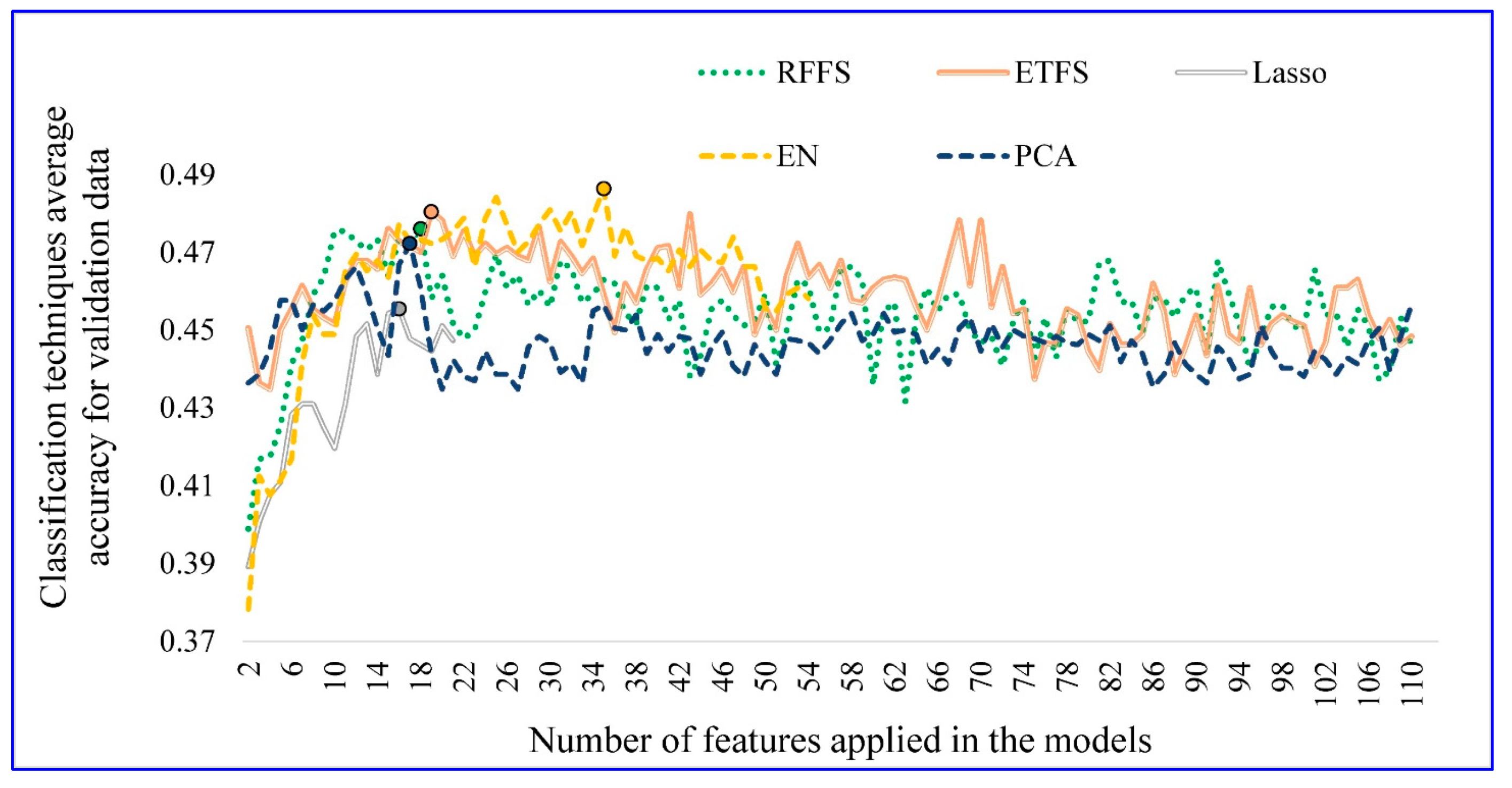
4.1. Optimal Number of Features

Initially, conventional feature selection techniques were ran, and feature importance weights were obtained. Then, the optimal number of features were tested incrementally from 2 to 110 by decreasing value of importance weight. All classifiers were run, and the average value of validation data accuracy was calculated for each possible optimal number of features and for each conventional feature selection technique. The results of this analysis are shown in Figure 2. As can be seen, the optimal number of features for RFFS, ETFS, Lasso, EN, and PCA were 18, 19, 16, 35, and 17, respectively. A more detailed look at this graph reveals that the applied method enhanced the performance of feature selection techniques, even for EN and Lasso that already determine the optimal number of features. The average accuracy of classifiers for EN and Lasso features were increased by 2.8% and 0.8% respectively by considering the introduced improvement to find the optimal number of features. Therefore, it can be inferred that the conventional versions of Lasso and EN do not present the optimal number of features if the introduced improvement technique is overlooked in their process. Additionally, these versions of RFFS, ETFS, and PCA can present the optimal number of features. It should be noted that there is not a direct correlation between increasing the number of features and an increase in the prediction accuracy. By increasing the number of features, the accuracy was increased until a threshold, and afterward, it reduced for all feature selection techniques. Thus, applying the improved versions to find the optimal number of features for conventional feature selection techniques in problems with a high number of features could be vital.

The optimal feature sets for all feature selection techniques were used to train all classifiers, and then the accuracy of the testing data was calculated to compare their performance. COA-QDA directly obtained the optimal number of features. The optimal number of features was determined to be 46 by COA-QDA. Furthermore, the optimal value of ${\alpha }_1$ and ${\alpha }_2$ was 1 and 2, respectively.

4.2. Feature Selection Technique Performance

The training and testing data accuracy of all classifiers for different feature selection techniques is shown in

Table 2. The accuracy of classifiers based on various feature selection technique’s optimal features.

Feature Selection Techniques	Data Type	MLP	NB	LR	DT	KNN	RF	SVM	AB	Average Accuracy	Maximum Accuracy	Accuracy Standard Deviation
All features	Training	0.461	0.528	0.623	0.570	0.438	0.979	0.838	0.519	0.620	0.979	0.179
	Testing	0.338	0.481	0.502	0.351	0.390	0.502	0.506	0.459	0.441	0.506	0.066
ETFS	Training	0.571	0.521	0.554	0.557	0.514	0.900	0.687	0.503	0.601	0.900	0.125
	Testing	0.498	0.476	0.494	0.446	0.407	0.494	0.468	0.494	0.472	0.498	0.030
EN	Training	0.735	0.505	0.561	0.554	0.497	0.935	0.754	0.515	0.632	0.935	0.149
	Testing	0.476	0.485	0.524	0.398	0.420	0.489	0.498	0.472	0.470	0.524	0.039
Lasso	Training	0.620	0.473	0.507	0.532	0.477	0.887	0.647	0.474	0.577	0.887	0.133
	Testing	0.437	0.433	0.455	0.416	0.394	0.481	0.437	0.398	0.431	0.481	0.027
RFFS	Training	0.556	0.491	0.517	0.559	0.473	0.914	0.659	0.479	0.581	0.914	0.138
	Testing	0.459	0.481	0.494	0.394	0.381	0.494	0.511	0.446	0.457	0.511	0.045
PCA	Training	0.620	0.408	0.470	0.548	0.473	0.927	0.627	0.477	0.569	0.927	0.153
	Testing	0.398	0.381	0.459	0.420	0.407	0.476	0.455	0.394	0.424	0.476	0.033
COA-QDA	Training	0.529	0.500	0.553	0.569	0.428	0.946	0.768	0.493	0.598	0.946	0.161
	Testing	0.494	0.506	0.537	0.433	0.385	0.506	0.502	0.472	0.479	0.537	0.046

. According to the results presented in Table 2, COA-QDA provided the highest average testing data accuracy, followed by ETFS, EN, RFFS, all features, Lasso, and PCA. That is to say, the average testing data accuracy of COA-QDA was 0.7%, 0.9%, 2.2%, 3.8%, 4.8%, and 5.6% higher than that of ETFS, EN, RFFS, all features, Lasso, and PCA, considering all classifiers, respectively. Thus, it can be inferred that COA-QDA is better at detecting the optimal features for CC-SoC prediction. Meanwhile, applying COA-QDA, ETFS, EN, RFFS could improve the average prediction accuracy compared with a model without using any feature selection. On the other hand, the average testing data accuracy of Lasso and PCA was lower than the all-features model, so the application of these feature selection techniques is not recommended for the CC-SoC prediction problem.

Drawing on the results presented in Table 2, the highest accuracy was obtained by COA-QDA, with a value of 53.7%. The maximum accuracy achieved by EN, RFFS, all features, ETFS, Lasso, and PCA were 1.3%, 2.6%, 3%, 3.9%, 5.6%, and 6.1% lower than COA-QDA, respectively. Hence, it can be proposed that COA-QDA outperformed other feature selection techniques based on obtaining the highest accuracy. The performance of EN and RFFS were also desirable as their maximum accuracy was higher than that of the all-features model. However, ETFS, Lasso, and PCA could not improve the accuracy if they were replaced with the model without using any feature selection.

Another purpose of the current study was to find the best combination of feature selection techniques and classifiers to achieve the highest prediction accuracy. For the column of Maximum accuracy in Table 2, the highest testing data accuracy was related to COA-QDA optimal features trained by logistic regression (COA-QDA/LR). The combination of COA-QDA and LR led to the highest testing data accuracy of 53.7%, followed by EN/LR, RFFS/SVM, COA-QDA/NB, COA-QDA/RF, and all features/SVM, with the values of 52.4%, 51.1%, 50.6%, 50.6%, and 50.6%, respectively.

Computational complexity is a vital criterion to compare different soft computing techniques., while running time is a straightforward method that is generally taken into consideration to compare different methods. To this end, the running time of feature selection techniques was evaluated and presented in Figure 3. The running time considered the whole-cycle running time, including running the method and the time spent on finding the optimal number of features. As can be seen from Figure 3, Lasso required the minimum time to find the optimal feature set. Lasso’s short running time may be due to removing a significant portion of features in the first step. Hence, in the second step, the number of runs for different classifiers is reduced considerably. EN was the second fastest feature selection technique. Hence, considering the average accuracy, maximum accuracy, and running time, EN is the best option among the conventional feature selection techniques. COA-QDA was the third fastest feature selection technique. Thus, the performance of COA-QDA is highly attractive considering its average testing data accuracy, highest testing data accuracy, and running time. Therefore, COA-QDA is found to be a competent approach to the CC-SoC prediction problem. PCA, RFFS, and ETFS were the fourth, fifth, and sixth algorithms based on running time ranking.

4.3. Classifiers’ Accuracy

The average testing data accuracy of different classifiers over different datasets, generated by various feature selection techniques, is presented in Figure 4. As can be seen, LR provided the highest average accuracy considering testing data. The average testing data accuracy of LR was 0.1%, 0.76%, 1.57%, 3.36%, 4%, 6.93%, and 7.26% higher than that of RF, SVM, NB, AB, MLP, KNN, and DT, respectively. The average testing data accuracy of all classifiers on all datasets was 42.51%. Considering this value (i.e., 42.51%) as a threshold, LR, RF, SVM, and NB can be considered appropriate classification techniques to predict CC-SoC. On the other hand, the average testing data accuracy of AB, MLP, KNN, and DT was less than the average prediction accuracy of all classifiers. Furthermore, it can be deduced that LR and RF outperformed other classifiers based on testing data average accuracy. In contrast, DT and KNN may not be appropriate techniques to predict CC-SoC as they obtained the lowest testing data accuracy.

4.4. The Most Important Features

As mentioned, one of the main purposes of this investigation is to detect the vital features that should be used in classifiers to obtain the highest prediction accuracy. Thus, COA-QDA/LR (LR trained by COA-QDA optimal features), as the most accurate model, is applied in the introduced sensitivity analysis to prioritize the optimal features. COA-QDA contained 46 features in the optimal features set. Each individual feature was eliminated from the dataset to test for its influence. The model was then run, and the average testing data accuracy reduction of all classifiers was calculated. In other words, the features were ranked based on their effects on the prediction accuracy reduction. The ranking of optimal features is presented in

Table 3. The optimal features for CC-SoC prediction and their corresponding feature groups.

Ranking	Questions (Features)	Group
1	What was your total household income before taxes during the past 12 months?	Socio-demographic
2	I buy milk in returnable bottles	GEB
3	How much would you be willing to pay per ton of additional GHG emissions?	Extra features
4	The production year of the current vehicle	Transport-related
5	I talk with friends about problems related to the environment	GEB
6	In summer, I turn the AC off when I leave my home for more than 4 h.	GEB
7	I own a fuel-efficient automobile	GEB
8	Government rules allow mini-vans, vans, pick-ups, and SUVs to pollute more than passenger cars, for every gallon of gas used	Extra features
9	For long trips (more than 6 h), I take an airplane.	GEB
10	Do you have the base model or do you have a model with optional upgrades?	Transport-related
11	Age	Socio-demographic
12	When do you expect to purchase (or lease) your next car?	Transport-related
13	I buy convenience foods	GEB
14	Please select the make of your car	Transport-related
15	What is your relationship status?	Socio-demographic
16	I reuse my shopping bags.	GEB
17	I have pointed out unecological behavior to someone.	GEB
18	How many people have driver licenses in your household (including you)?	Socio-demographic
19	What is your gender?	Socio-demographic
20	Human destruction of the natural environment has been greatly exaggerated.	NEP
21	We are approaching the limit of the number of people the earth can support.	NEP
22	How many people are in your household including you?	Socio-demographic
23	I buy beverages in cans	GEB
24	Plants and animals have as much right as humans to exist	NEP
25	I wait until I have a full load before doing my laundry	GEB
26	I put dead batteries in the garbage.	GEB
27	If I am offered a plastic bag in a store, I take it.	GEB
28	How long would you plan on keeping your next car?	Transport-related
29	Current car annual mileage	Transport-related
30	Will you purchase or lease your next car?	Transport-related
31	After meals, I throw leftovers in the garbage disposal.	GEB
32	How often do you commute by car?	Transport-related
33	Describe your housing type	Socio-demographic
34	I drive my car into the city	GEB
35	All cars, mini-vans, vans, pickups, and SUVs pollute about the same amount for each mile driven.	Extra features
36	In hotels, I have the towels changed daily.	GEB
37	Please select the model of your car	Transport-related
38	When humans interfere with nature it often produces disastrous consequences	NEP
39	I am a member of a carpool.	GEB
40	I bought solar panels to produce energy	GEB
41	I drive in such a way as to keep my fuel consumption as low as possible	GEB
42	I requested an estimate on having solar power installed	GEB
43	The earth has plenty of natural resources if we just learn how to develop them	NEP
44	If things continue on their present course, we will soon experience a major ecological disaster	NEP
45	For distances up to 20 miles, I use public transport	GEB
46	I bring empty bottles to a recycling bin	GEB

.

As can be seen from Table 3, the portion of GEB, transport-related, socio-demographic, NEP, and extra features in the optimal feature set is 45.7%, 19.6%, 15.2%, 13%, and 6.5%. Before highlighting the transportation features, we should point out the sample only contained Americans who owned at least one car. In this sample, the production year of the current vehicle was the most important transport-related feature on CC-SoC prediction. Similarly, availability of a car with optional upgrades, expectation time to buy or lease a new car, current car makes, the expected time to keep the next car, annual mileage driving, selecting between purchase or lease, frequency of using a car, and model of the current car were selected in the optimal feature sets, and they should be applied in order to generate an accurate CC-SoC prediction model. Interestingly, six GEB questions in the optimal set were based on transport behavior. Owning a fuel-efficient car, taking a plane for long trips, driving the car into the city, being a member of a carpool, driving in such a way as to keep one’s fuel consumption as low as possible, and using public transport for distances up to 20 miles were the transport-based GEB questions that were selected as the optimal features. Thus, 32.6% of features were related to transport behavior considering transport-related and GEB questions. Therefore, it can be postulated that transport-related behavior can be considered as climate-change related indices, and they should be applied to predict CC-SoC.

4.5. Comparing the Results with Previous Studies

Ramachandran et al. [62] compared the performance of random forest classifier and logistic regression on predicting an ordinal variable (fall detection in geriatric healthcare systems). Their study showed that logistic regression outperformed random forest classifier based on prediction accuracy on ordinal variable prediction, which is in line with the outcomes of the current study. Meti et al. [63] applied five machine learning techniques, including Random Forest classifier, Support Vector Machine, K-Nearest Neighbor classifier, Multi-Layered Perceptron, and Naive Bayes, to predict neoadjuvant chemotherapy response in breast cancer. Subsequently, they compared the prediction accuracy of the mentioned classifiers, and the results indicated that the random forest classifier had a better prediction performance than the other machine learning techniques. Hence, their results are in harmony with the results of this study, shown in Figure 3.

In another study, Vanhoenshoven et al. [64] compared the performance of different classification techniques, including Multi-Layer Perceptron, Naïve Bayes, Decision Trees, k-Nearest Neighbors, Random Forest Classifier, and Support Vector Machines, on a binary classification problem. The results demonstrated that Random Forest Classifier was the best classifier in terms of prediction accuracy, which is consistent with the results of this investigation.

Ahmad et al. [65] employed k-Nearest Neighbors, Multi-Layer Perceptron, Naïve Bayes, Random Forest Classifier, and Support Vector Machine to model a gender recognition task problem. Comparing the prediction accuracy of classifiers revealed that Support Vector Machine was the best classifier to predict gender using speech. Therefore, this outcome contradicts the results of the current study that SVM could not perform well. This contradiction is due to the difference in prediction problems’ output. That is, the prediction output variable of this study is an ordinal variable, while a binary variable (i.e., gender) was considered the prediction output in Ahmad et al. [65] study.

5. Conclusions

This study proposed a new AI approach that was applied to predict individual CC-SoC. Behaviors such as recycling may be more commonly thought of as environmental, but transport must be considered as it is a major contributor of CO₂ emissions. As such, so transport’s role in predicting CC-SoC was examined. Transport-related behaviors, socio-demographic characteristics, General Environmental Behaviors (GEB; established tool for measuring environmental attitudes and behavior), and New Environmental Paradigm (NEP; established tool for measuring environmental attitudes) features were all employed to generate a prediction model. As the model included several features (variables), a new feature selection technique was introduced to find the optimal number of features and optimal features to obtain the highest accuracy. Different conventional feature selection methods, including Lasso, Elastic Net, Random Forest Feature Selection, Extra Trees, and Principal component analysis feature selection, were used to select the most valuable feature selections. Moreover, a new approach was presented to improve the performance of conventional feature selection techniques and find their optimal feature sets. Consequently, eight different classification techniques were applied to achieve the highest accuracy. Ultimately, a sensitivity analysis was utilized to prioritize and rank the optimal features. The main conclusions are as follows:

• Fifteen optimal features (out of forty-six) are based on transport behavior: nine from transport-related questions and six from GEB transport-based questions. Hence, 32.6% of optimal features are related to transport behavior. This suggests that the application of transport behavior to predict CC-SoC is vital. It should be noted that the original survey focus was on vehicle choice and included only car owners. As such, future research should examine a larger array of transport behaviors with a general population sample.
• The introduced improvement method for conventional feature selection models can increase the average prediction accuracy of EN and Lasso by 2.8% and 0.8%, respectively. RFFS, ETFS, and PCA can also determine the optimal number of features using the proposed improvement method.
• The average testing data accuracy of COA-QDA is 0.7%, 0.9%, 2.2%, 4.8%, and 5.6% higher than that of ETFS, EN, RFFS, Lasso, and PCA. Accordingly, COA-QDA outperforms other feature selection techniques in terms of accuracy. Using an appropriate feature selection technique, such as COA-QDA, can increase the average accuracy by 3.8% as compared to not using all features in the model.
• COA-QDA provides the highest testing accuracy, with a value of 53.7%. The highest COA-QDA testing data accuracy is 1.3%, 2.6%, 3.9%, 5.6%, and 6.1% higher than that of EN, RFFS, ETFS, Lasso, and PCA, respectively. Furthermore, using all features in the prediction models results in a model with 3% lower testing data accuracy than COA-QDA.
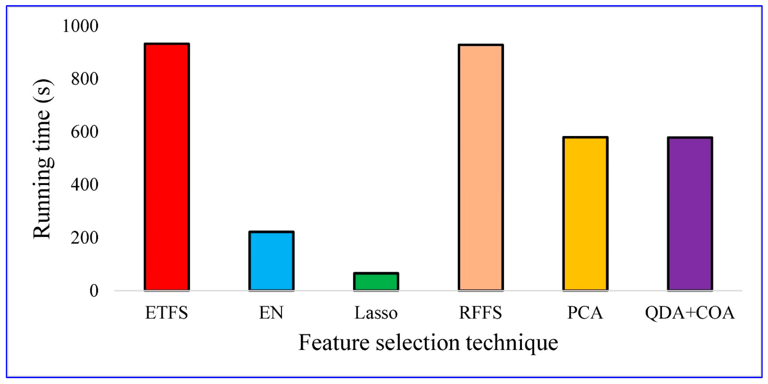
• Lasso is the fastest feature selection method regarding the average running time, followed by EN, COA-QDA, PCA, RFFS, and ETFS.
• The highest testing data accuracy is obtained by combining COA-QDA and LR (COA-QDA/LR), followed by EN/LR, RFFS/SVM, COA-QDA/NB, COA-QDA/RF, and all features/SVM. The testing data accuracy these methods is equal to 53.7%, 52.4%, 51.1%, 50.6%, 50.6%, and 50.6%, respectively. This may be a result of the type of dependent variable (ordinal).
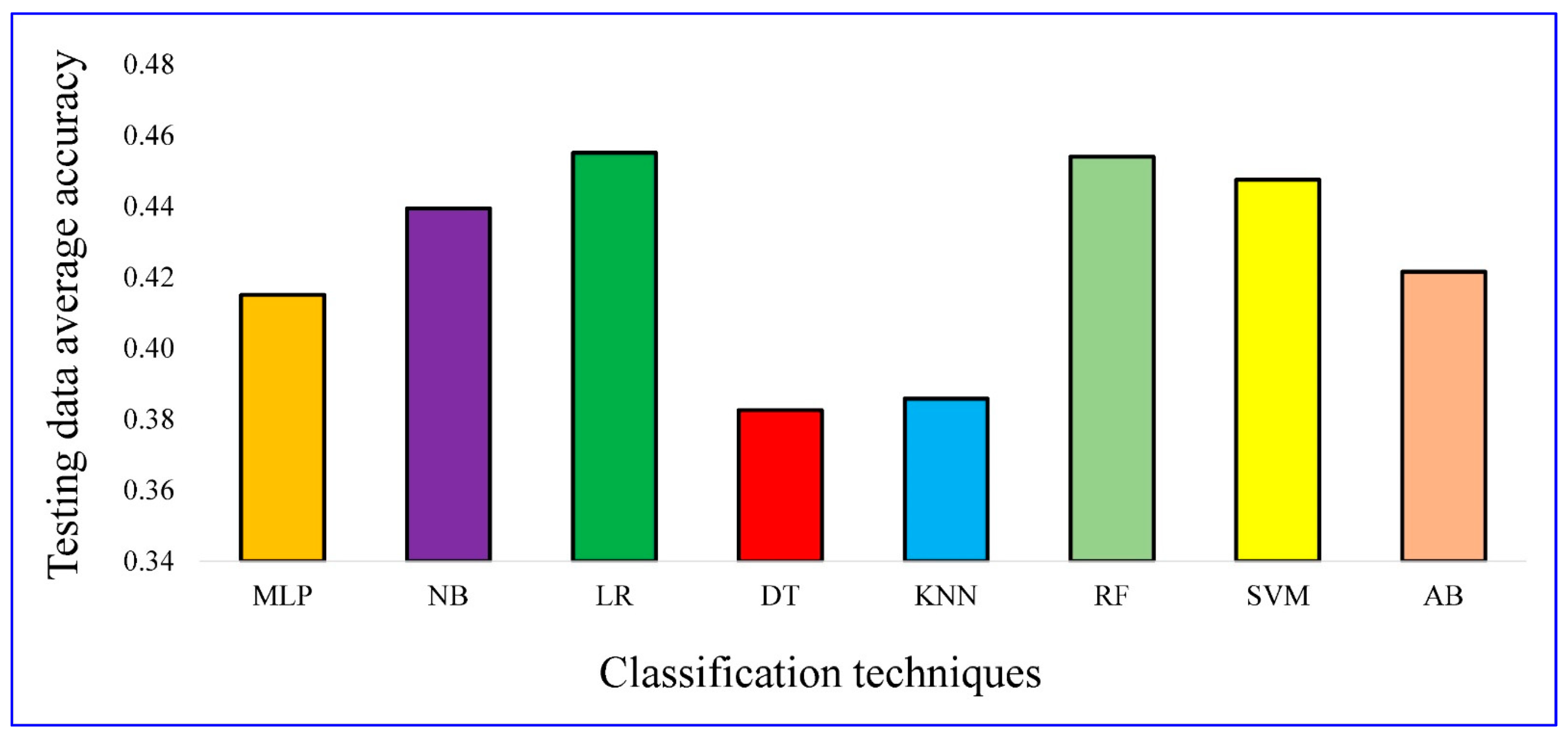
• The average testing data accuracy of LR, RF, SVM, NB, AB, MLP, KNN, DT is 45.5%, 45.4%, 44.8%, 43.9%, 42.2%, 41.5% 38.6%, and 38.3%, in the order given. Therefore, in this study LR and RF outperformed other classifiers based on the average prediction accuracy.

6. Limitations and Recommendations for Future Studies

The limitations of this study and some recommendations for considering in future studies are presented in this section:

• The measure, Climate Change Stage of Change, captures individuals’ self-assessment of their climate concern and behavioral intentions. It does measure what their actual climate impacts are. It is possible for a person not to be concerned about climate change and lead a low-carbon lifestyle. It should only be considered with respect to how strongly they would likely support or react to climate-related information.
• In this study, the performance of COA-QDA is only examined on the CC-SoC prediction study. Accordingly, it is recommended that assessing the performance of COA-QDA on different prediction problems with different complexities will be considered in future studies.
• This study applies Coyote Optimization Algorithm to propose a feature selection method (i.e., COA-QDA). Hence, it is suggested to employ various robust metaheuristic algorithms to generate new feature selection methods using the proposed approach.
• One of the limitations of this study is to consider testing data accuracy as the performance indicator. It is recommended that the effects of COA-QDA on testing data F1-score will be examined in future studies.

References

1. McCright, A.M.; Marquart-Pyatt, S.T.; Shwom, R.L.; Brechin, S.R.; Allen, S. Ideology, capitalism, and climate: Explaining public views about climate change in the United States. Energy Res. Soc. Sci. 2016, 21, 180–189. [Google Scholar] [CrossRef]
2. Yang, M.X.; Tang, X.; Cheung, M.L.; Zhang, Y. An institutional perspective on consumers’ environmental awareness and pro-environmental behavioral intention: Evidence from 39 countries. Bus. Strat. Environ. 2020, 30, 566–575. [Google Scholar] [CrossRef]
3. Anable, J. ‘Complacent Car Addicts’ or ‘Aspiring Environmentalists’? Identifying travel behaviour segments using attitude theory. Transp. Policy 2005, 12, 65–78. [Google Scholar] [CrossRef] [Green Version]
4. Susilo, Y.O.; Williams, K.; Lindsay, M.; Dair, C. The influence of individuals’ environmental attitudes and urban design features on their travel patterns in sustainable neighborhoods in the UK. Transp. Res. Part D Transp. Environ. 2012, 17, 190–200. [Google Scholar] [CrossRef] [Green Version]
5. Gaker, D.; Walker, J.L. Revealing the Value of “Green” and the Small Group with a Big Heart in Transportation Mode Choice. Sustainability 2013, 5, 2913–2927. [Google Scholar] [CrossRef] [Green Version]
6. Wynes, S.; Nicholas, K.A. The climate mitigation gap: Education and government recommendations miss the most effective individual actions. Environ. Res. Lett. 2017, 12, 074024. [Google Scholar] [CrossRef] [Green Version]
7. Waygood, E.O.D.; Wang, B.; Daziano, R.A.; Patterson, Z.; Kohlová, M.B. The climate change stage of change measure: Vehicle choice experiment. J. Environ. Plan. Manag. 2021, 1–30. [Google Scholar] [CrossRef]
8. Prochaska, J.; Colleen, O.; Redding, A.; Evers, K.E. The transtheoretical model and stages of change. In Health Behavior: Theory, Research, and Practice; John Wiley & Sons: San Francisco, CA, USA, 2015. [Google Scholar]
9. Waygood, E.; Avineri, E. Does “500g of CO2 for a mile trip” mean anything? Towards more effective presentation of CO2 Information. In Proceedings of the Transportation Research Board 90th Annual Meeting, Washington, DC, USA, 23–27 January 2011. [Google Scholar]
10. Daziano, R.A.; Waygood, E.O.D.; Patterson, Z.; Kohlová, M.B. Increasing the influence of CO2 emissions information on car purchase. J. Clean. Prod. 2017, 164, 861–871. [Google Scholar] [CrossRef] [Green Version]
11. Wang, B.; Waygood, E.; Daziano, R.A.; Patterson, Z.; Feinberg, M. Does hedonic framing improve people’s willingness-to-pay for vehicle greenhouse gas emissions? Transp. Res. Part D Transp. Environ. 2021, 98, 102973. [Google Scholar] [CrossRef]
12. Waygood, E.O.; Wang, B.; Daziano, R.A.; Patterson, Z.; Kohlová, M.B. Vehicle choice and CO2 emissions information: Framing effects and individual climate change stage of change. In Proceedings of the Annual Meeting Transportation Research Board, Washington, DC, USA, 12–16 January 2020. [Google Scholar]
13. Zha, D.; Yang, G.; Wang, W.; Wang, Q.; Zhou, D. Appliance energy labels and consumer heterogeneity: A latent class approach based on a discrete choice experiment in China. Energy Econ. 2020, 90, 104839. [Google Scholar] [CrossRef]
14. Bedard, S.A.N.; Tolmie, C.R. Millennials’ green consumption behaviour: Exploring the role of social media. Corp. Soc. Responsib. Environ. Manag. 2018, 25, 1388–1396. [Google Scholar] [CrossRef]
15. Cheung, M.L.; Pires, G.D.; Rosenberger, P.J.; Leung, W.K.; Sharipudin, M.-N.S. The role of consumer-consumer interaction and consumer-brand interaction in driving consumer-brand engagement and behavioral intentions. J. Retail. Consum. Serv. 2021, 61, 102574. [Google Scholar] [CrossRef]
16. Liu, Y.; Cirillo, C. A generalized dynamic discrete choice model for green vehicle adoption. Transp. Res. Part A Policy Pract. 2018, 114, 288–302. [Google Scholar] [CrossRef]
17. Wang, S.; Mo, B.; Hess, S.; Zhao, J. Comparing hundreds of machine learning classifiers and discrete choice models in predicting travel behavior: An empirical benchmark. arXiv 2021, arXiv:2102.01130. [Google Scholar]
18. Lee, D.; Kang, S.; Shin, J. Using Deep Learning Techniques to Forecast Environmental Consumption Level. Sustainability 2017, 9, 1894. [Google Scholar] [CrossRef] [Green Version]
19. Amasyali, K.; El-Gohary, N. Machine learning for occupant-behavior-sensitive cooling energy consumption prediction in office buildings. Renew. Sustain. Energy Rev. 2021, 142, 110714. [Google Scholar] [CrossRef]
20. Lee, D.; Kim, M.; Lee, J. Adoption of green electricity policies: Investigating the role of environmental attitudes via big data-driven search-queries. Energy Policy 2016, 90, 187–201. [Google Scholar] [CrossRef]
21. Ping, P.; Qin, W.; Xu, Y.; Miyajima, C.; Takeda, K. Impact of Driver Behavior on Fuel Consumption: Classification, Evaluation and Prediction Using Machine Learning. IEEE Access 2019, 7, 78515–78532. [Google Scholar] [CrossRef]
22. Chang, X.; Wu, J.; Liu, H.; Yan, X.; Sun, H.; Qu, Y. Travel mode choice: A data fusion model using machine learning methods and evidence from travel diary survey data. Transp. A Transp. Sci. 2019, 15, 1587–1612. [Google Scholar] [CrossRef]
23. Wade, B.S.; Joshi, S.H.; Gutman, B.A.; Thompson, P.M. Machine learning on high dimensional shape data from subcortical brain surfaces: A comparison of feature selection and classification methods. Pattern Recognit. 2017, 63, 731–739. [Google Scholar] [CrossRef]
24. Sanchez-Pinto, L.N.; Venable, L.R.; Fahrenbach, J.; Churpek, M.M. Comparison of variable selection methods for clinical predictive modeling. Int. J. Med. Inform. 2018, 116, 10–17. [Google Scholar] [CrossRef]
25. Climate Watch. Global GHG Emissions. Available online: https://www.climatewatchdata.org (accessed on 20 May 2018).
26. Kaiser, F.; Wilson, M.R. Goal-directed conservation behavior: The specific composition of a general performance. Pers. Individ. Differ. 2004, 36, 1531–1544. [Google Scholar] [CrossRef]
27. Dunlap, R.E.; Van Liere, K.D.; Mertig, A.G.; Jones, R.E. New Trends in Measuring Environmental Attitudes: Measuring Endorsement of the New Ecological Paradigm: A Revised NEP Scale. J. Soc. Issues 2000, 56, 425–442. [Google Scholar] [CrossRef]
28. Majidifard, H.; Jahangiri, B.; Rath, P.; Contreras, L.U.; Buttlar, W.G.; Alavi, A.H. Developing a prediction model for rutting depth of asphalt mixtures using gene expression programming. Constr. Build. Mater. 2020, 267, 120543. [Google Scholar] [CrossRef]
29. Naseri, H.; Jahanbakhsh, H.; Khezri, K.; Shirzadi Javid, A.A. Toward sustainability in optimizing the fly ash concrete mixture ingredients by introducing a new prediction algorithm. Environ. Dev. Sustain. 2021. [Google Scholar] [CrossRef]
30. Hasan, K.; Alam, A.; Das, D.; Hossain, E.; Hasan, M. Diabetes Prediction Using Ensembling of Different Machine Learning Classifiers. IEEE Access 2020, 8, 76516–76531. [Google Scholar] [CrossRef]
31. Ontivero-Ortega, M.; Lage-Castellanos, A.; Valente, G.; Goebel, R.; Valdes-Sosa, M. Fast Gaussian Naïve Bayes for searchlight classification analysis. NeuroImage 2017, 163, 471–479. [Google Scholar] [CrossRef] [PubMed]
32. Dong, L.; Wesseloo, J.; Potvin, Y.; Li, X. Discrimination of Mine Seismic Events and Blasts Using the Fisher Classifier, Naive Bayesian Classifier and Logistic Regression. Rock Mech. Rock Eng. 2015, 49, 183–211. [Google Scholar] [CrossRef]
33. Hajmeer, M.; Basheer, I. Comparison of logistic regression and neural network-based classifiers for bacterial growth. Food Microbiol. 2003, 20, 43–55. [Google Scholar] [CrossRef]
34. Suresh, A.; Udendhran, R.; Balamurgan, M. Hybridized neural network and decision tree based classifier for prognostic decision making in breast cancers. Soft Comput. 2019, 24, 7947–7953. [Google Scholar] [CrossRef]
35. Rau, C.-S.; Wu, S.-C.; Chien, P.-C.; Kuo, P.-J.; Cheng-Shyuan, R.; Hsieh, H.-Y.; Hsieh, C.-H. Prediction of Mortality in Patients with Isolated Traumatic Subarachnoid Hemorrhage Using a Decision Tree Classifier: A Retrospective Analysis Based on a Trauma Registry System. Int. J. Environ. Res. Public Health 2017, 14, 1420. [Google Scholar] [CrossRef] [Green Version]
36. Duca, A.L.; Bacciu, C.; Marchetti, A. A K-nearest neighbor classifier for ship route prediction. In Proceedings of the OCEANS 2017—Aberdeen, Aberdeen, UK, 19–22 June 2017; pp. 1–6. [Google Scholar] [CrossRef]
37. Noi, P.T.; Kappas, M. Comparison of Random Forest, k-Nearest Neighbor, and Support Vector Machine Classifiers for Land Cover Classification Using Sentinel-2 Imagery. Sensors 2017, 18, 18. [Google Scholar] [CrossRef] [Green Version]
38. Dogru, N.; Subasi, A. Traffic accident detection using random forest classifier. In Proceedings of the 2018 15th Learning and Technology Conference (L&T), Jeddah, Saudi Arabia, 25–26 February 2018. [Google Scholar]
39. Chapleau, R.; Gaudette, P.; Spurr, T. Application of Machine Learning to Two Large-Sample Household Travel Surveys: A Characterization of Travel Modes. Transp. Res. Rec. J. Transp. Res. Board 2019, 2673, 173–183. [Google Scholar] [CrossRef]
40. Fan, J.; Wang, X.; Zhang, F.; Ma, X.; Wu, L. Predicting daily diffuse horizontal solar radiation in various climatic regions of China using support vector machine and tree-based soft computing models with local and extrinsic climatic data. J. Clean. Prod. 2020, 248, 119264. [Google Scholar] [CrossRef]
41. Li, L.-L.; Zhao, X.; Tseng, M.-L.; Tan, R.R. Short-term wind power forecasting based on support vector machine with improved dragonfly algorithm. J. Clean. Prod. 2020, 242, 118447. [Google Scholar] [CrossRef]
42. Hu, G.; Yin, C.; Wan, M.; Zhang, Y.; Fang, Y. Recognition of diseased Pinus trees in UAV images using deep learning and AdaBoost classifier. Biosyst. Eng. 2020, 194, 138–151. [Google Scholar] [CrossRef]
43. Pierezan, J.; Coelho, L.D.S. Coyote optimization algorithm: A new metaheuristic for global optimization problems. In Proceedings of the 2018 IEEE Congress on Evolutionary Computation (CEC), Rio de Janeiro, Brazil, 8–13 July 2018. [Google Scholar] [CrossRef]
44. Pierezan, J.; Maidl, G.; Yamao, E.M.; Coelho, L.D.S.; Mariani, V.C. Cultural coyote optimization algorithm applied to a heavy duty gas turbine operation. Energy Convers. Manag. 2019, 199, 111932. [Google Scholar] [CrossRef]
45. Pierezan, J.; Coelho, S.; Mariani, V.C.; Lebensztajn, L. Multiobjective Coyote Algorithm Applied to Electromagnetic Optimization. In Proceedings of the 2019 22nd International Conference Computation of Electromagnetic Fields, Paris, France, 15–19 July 2019; pp. 1–4. [Google Scholar]
46. Naseri, H.; Ehsani, M.; Golroo, A.; Nejad, F.M. Sustainable pavement maintenance and rehabilitation planning using differential evolutionary programming and coyote optimisation algorithm. Int. J. Pavement Eng. 2021, 1–18. [Google Scholar] [CrossRef]
47. Srivastava, S.; Gupta, M.R.; Frigyik, B.A. Bayesian quadratic discriminant analysis. J. Mach. Learn. Res. 2007, 8, 1277–1305. [Google Scholar]
48. Kim, K.S.; Choi, H.H.; Moon, C.S.; Mun, C.W. Comparison of k-nearest neighbor, quadratic discriminant and linear discriminant analysis in classification of electromyogram signals based on the wrist-motion directions. Curr. Appl. Phys. 2011, 11, 740–745. [Google Scholar] [CrossRef]
49. Naseri, H.; Shokoohi, M.; Jahanbakhsh, H.; Golroo, A.; Gandomi, A.H. Evolutionary and swarm intelligence algorithms on pavement maintenance and rehabilitation planning. Int. J. Pavement Eng. 2021, 1–16. [Google Scholar] [CrossRef]
50. Naseri, H.; Fani, A.; Golroo, A. Toward equity in large-scale network-level pavement maintenance and rehabilitation scheduling using water cycle and genetic algorithms. Int. J. Pavement Eng. 2020, 1–13. [Google Scholar] [CrossRef]
51. Naseri, H.; Jahanbakhsh, H.; Hosseini, P.; Nejad, F.M. Designing sustainable concrete mixture by developing a new machine learning technique. J. Clean. Prod. 2020, 258, 120578. [Google Scholar] [CrossRef]
52. Tibshirani, R. Regression Shrinkage and Selection Via the Lasso. J. R. Stat. Soc. Ser. B 1996, 58, 267–288. [Google Scholar] [CrossRef]
53. Muthukrishnan, R.; Rohini, R. LASSO: A feature selection technique in predictive modeling for machine learning. In Proceedings of the 2016 IEEE International Conference on Advances in Computer Applications (ICACA), Coimbatore, India, 24 October 2016. [Google Scholar]
54. Fonti, V. Feature Selection Using LASSO; VU Amsterdam: Amsterdam, The Netherlands, 2017. [Google Scholar]
55. Cui, L.; Bai, L.; Wang, Y.; Jin, X.; Hancock, E.R. Internet financing credit risk evaluation using multiple structural interacting elastic net feature selection. Pattern Recognit. 2021, 114, 107835. [Google Scholar] [CrossRef]
56. Zou, H.; Hastie, T. Regularization and variable selection via the elastic net. J. R. Stat. Soc. Ser. B 2005, 67, 301–320. [Google Scholar] [CrossRef] [Green Version]
57. Jaiswal, J.K.; Samikannu, R. Application of Random Forest Algorithm on Feature Subset Selection and Classification and Regression. In Proceedings of the 2017 World Congress on Computing and Communication Technologies (WCCCT), Tiruchirappalli, India, 2–4 February 2017; pp. 65–68. [Google Scholar] [CrossRef]
58. Yamauchi, T. Mouse trajectories and state anxiety: Feature selection with random forest. In Proceedings of the 2013 Humaine Association Conference on Affective Computing and Intelligent Interaction, Geneva, Switzerland, 2–5 September 2013. [Google Scholar]
59. Sharma, J.; Giri, C.; Granmo, O.-C.; Goodwin, M.; Sharma, J.; Giri, C.; Granmo, O.-C.; Goodwin, M. Multi-layer intrusion detection system with ExtraTrees feature selection, extreme learning machine ensemble, and softmax aggregation. EURASIP J. Inf. Secur. 2019, 2019, 15. [Google Scholar] [CrossRef] [Green Version]
60. Guo, Q.; Wu, W.; Massart, D.; Boucon, C.; de Jong, S. Feature selection in principal component analysis of analytical data. Chemom. Intell. Lab. Syst. 2002, 61, 123–132. [Google Scholar] [CrossRef]
61. Song, F.; Guo, Z.; Mei, D. Feature selection using principal component analysis. In Proceedings of the 2010 International Conference on System Science, Engineering Design and Manufacturing Informatization, Yichang, China, 12–14 November 2010. [Google Scholar]
62. Ramachandran, A.; Anupama, K.R.; Adarsh, R.; Pahwa, P. Machine learning-based techniques for fall detection in geriatric healthcare systems. In Proceedings of the 2018 9th International Conference on Information Technology in Medicine and Education (ITME), Hangzhou, China, 19–21 October 2018; pp. 232–237. [Google Scholar]
63. Meti, N.; Saednia, K.; Lagree, A.; Tabbarah, S.; Mohebpour, M.; Kiss, A.; Lu, F.-I.; Slodkowska, E.; Gandhi, S.; Jerzak, K.J.; et al. Machine Learning Frameworks to Predict Neoadjuvant Chemotherapy Response in Breast Cancer Using Clinical and Pathological Features. JCO Clin. Cancer Inform. 2021, 5, 66–80. [Google Scholar] [CrossRef]
64. Vanhoenshoven, F.; Napoles, G.; Falcon, R.; Vanhoof, K.; Koppen, M. Detecting malicious URLs using machine learning techniques. In Proceedings of the 2016 IEEE Symposium Series on Computational Intelligence (SSCI), Athens, Greece, 6–9 December 2016. [Google Scholar]
65. Ahmad, J.; Fiaz, M.; Kwon, S.; Sodanil, M.; Vo, B.; Baik, S.W. Gender Identification using MFCC for Telephone Applications—A Comparative Study. arXiv 2016, arXiv:1601.01577. [Google Scholar]
Figure 1. The methodology flowchart.
Sustainability 14 00040 g001
Figure 2. The average validation data accuracy of classifiers by considering different values as the optimal number of features.
Sustainability 14 00040 g002
Figure 3. Whole cycle running time of feature selection techniques.
Sustainability 14 00040 g003
Figure 4. The average testing data accuracy of different classification techniques.
Sustainability 14 00040 g004