
Improving the Resilience of Port–Hinterland Container Logistics Transportation Systems: A Bi-Level Programming Approach

Abstract
:1. Introduction
- (1)
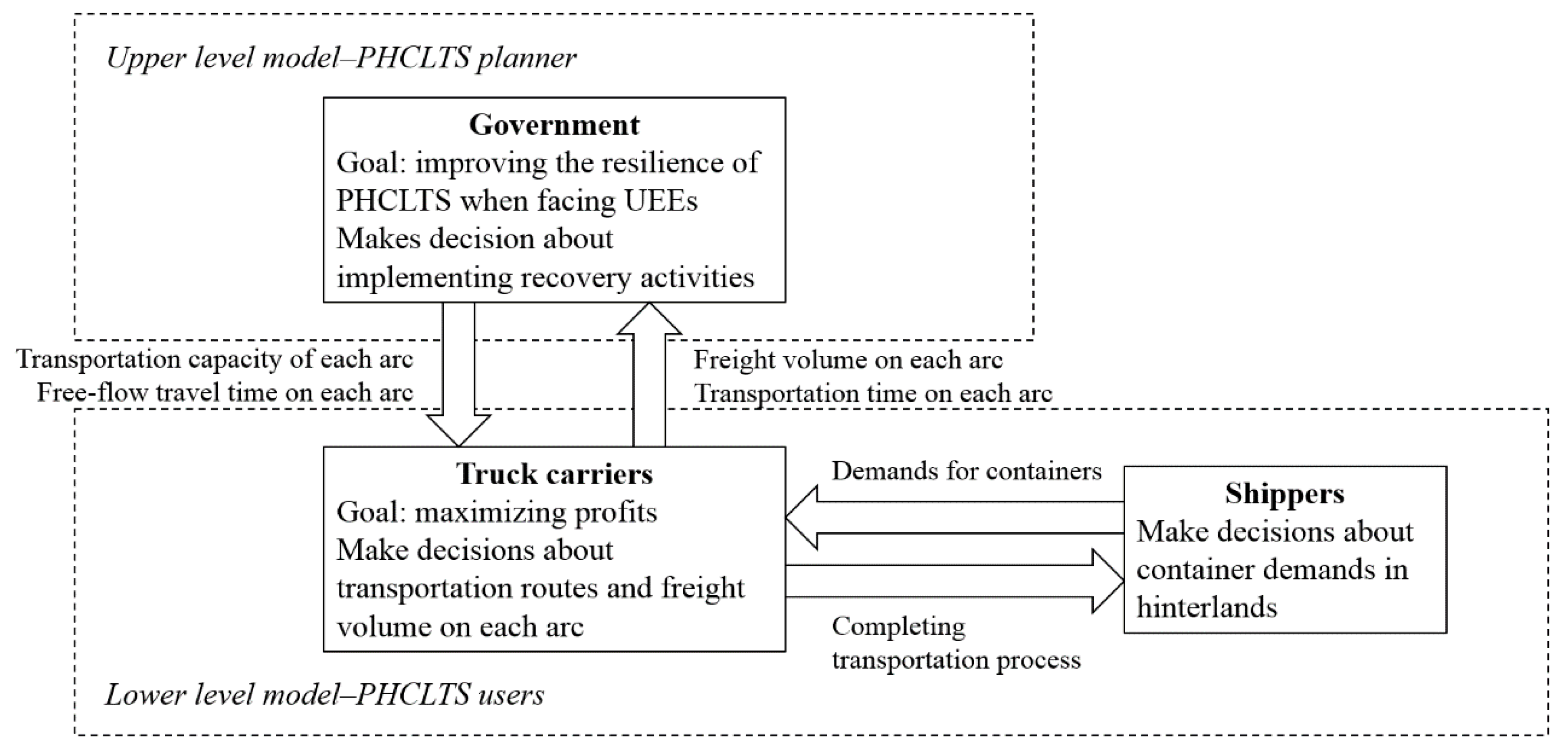
- Time resilience is adopted to measure and improve the resilience of a PHCLTS with considerations of PHCLTS user behaviors and the hierarchical relationship and interaction of government and truck carriers.
- (2)
- Bi-level programming models with two different lower level models are established according to different behavior patterns of PHCLTS users, supporting the government in selecting a reasonable budget level and implementing efficient recovery decisions to aid the PHCLTS to recover the operational capacity in the face of UEEs.
- (3)
- It expands the prearranged planning about UEEs and provides a decision-making reference and scientific theoretical support for an efficient response to UEEs.
2. Literature Review
2.1. Resilience of Transportation Systems
2.2. Logistics Transportation System Assignment and Equilibrium
2.3. Bi-Level Programming Model for Logistics Transportation System Problems
2.4. Summary of Literature Review
3. Model
3.1. Model Description and Assumptions
- (1)
- The daily transportation demands of containers are constant and unaffected by UEEs.
- (2)
- All containers are homogeneous, are the same size, and have the same value of goods loaded.
- (3)
- A recovery activity is implemented only once for each attacked arc in a PHCLTS.
- (4)
- The government has sufficient time to complete the recovery activities.
- (5)
- Road impedance exists in the PHCLTS.
3.2. Time Resilience of a PHCLTS
3.3. Model Formulation
3.3.1. Upper Level Model
3.3.2. Lower Level Model 1: The SO Model
3.3.3. Lower Level Model 2: The UE Model
4. Solution Algorithm
4.1. Description of Standard PSO
- (1)
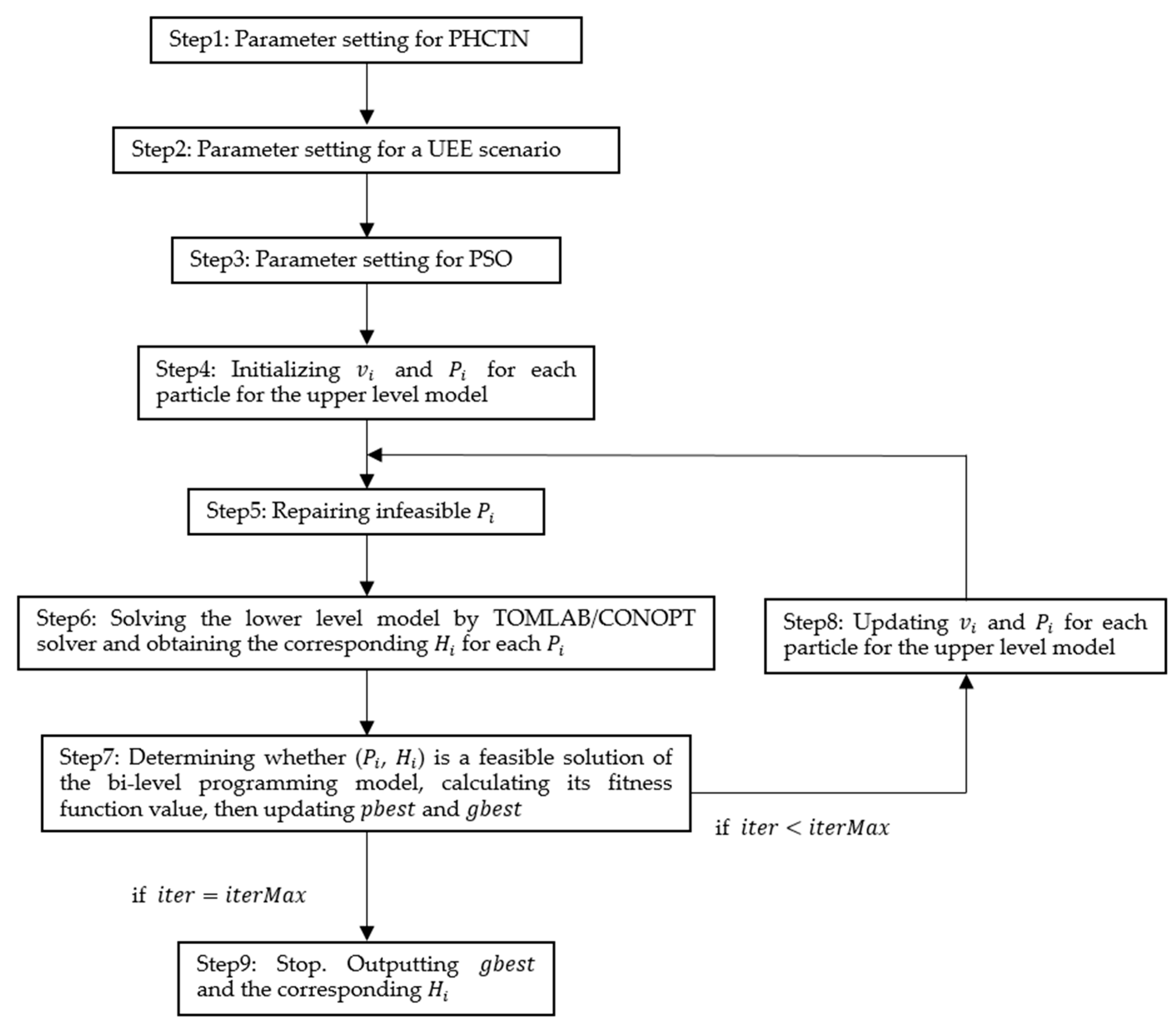
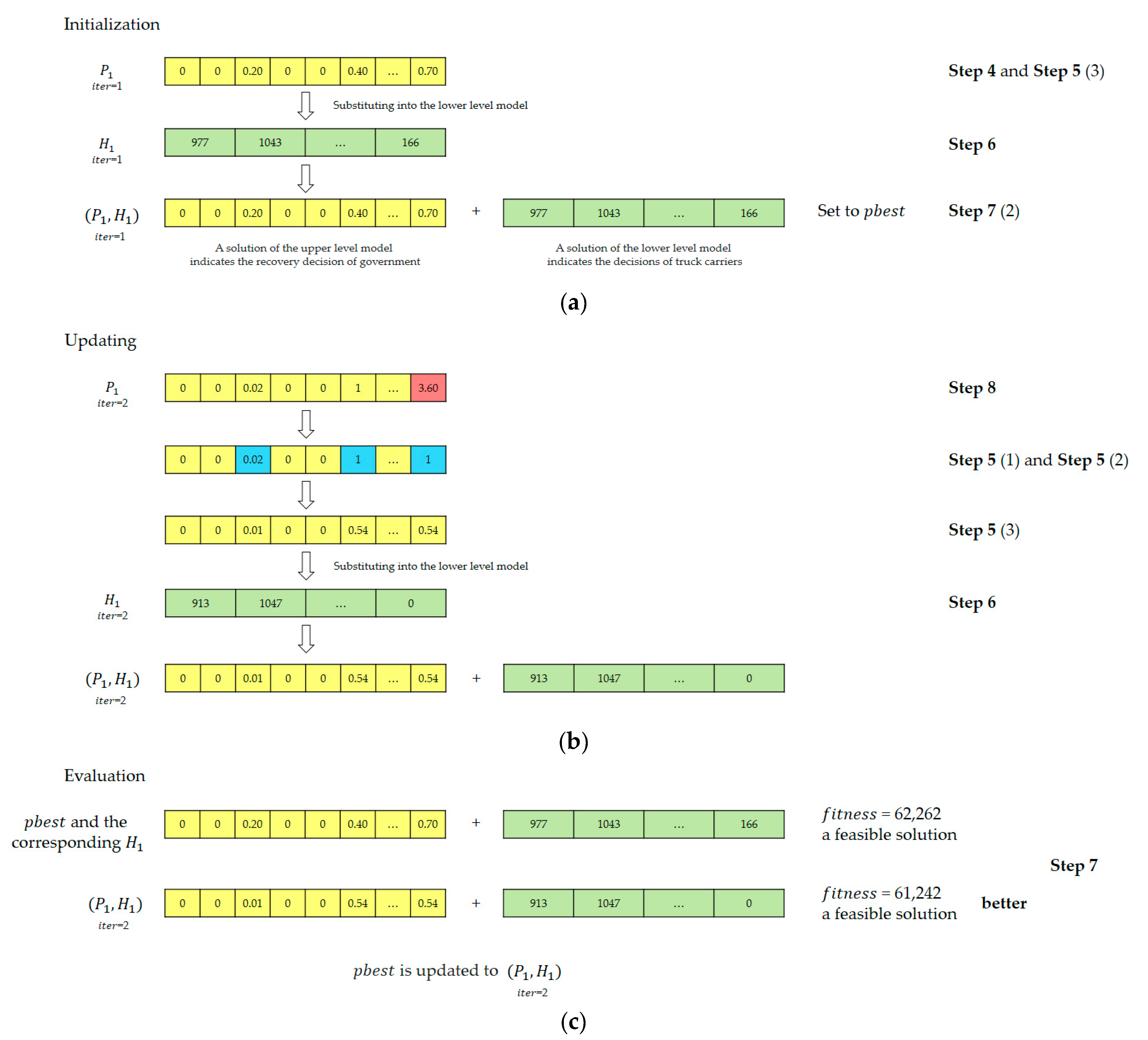
- The velocity vi and position Pi of particle i of the particle swarm are initialized through random generation, . Each particle i corresponds to a solution of the model needed to be solved. A fitness function is adopted to evaluate the particle. The position Pi of each particle i in the initialized population is set to pbest, . The particle with the best fitness function value is set to gbest.
- (2)
- In each iteration, Equations (17) and (18) are adopted to update the velocity vi and position Pi of particle i to generate a newswarm, .where w is the inertia weight. According to Shi [34], when w decreases linearly as the iteration increases, the convergence performance of the PSO algorithm will be improved. The following equation is adopted to calculate the value of w in each iteration:
- (3)
- The iteration process is repeated until the algorithm termination condition is reached, then the gbest is output to be solution of the model.
4.2. An Algorithm Combining PSO and Traditional Optimization Algorithms
- (1)
- The initial velocity vi for each particle i, , is randomly generated with a restriction of −4 to 4. In the subsequent iterations, the restrictions of particle velocities are removed due to the adopted inertia weight w [38].
- (2)
- (1)
- For Constraint (5), , if pi,a > 1, then it is adjusted to pi,a = 1; if pi,a < 0, then it is adjusted to pi,a = 0.
- (2)
- For Constraint (6), , if , then it is adjusted to pi,a = 0.
- (3)
- For Constraint (4), if position Pi does not meet this budget constraint, the corresponding total implementation cost of recovery activities for position Pi is calculated as
- (1)
- The capacity and free-flow travel time of arc a after recovery, and , are calculated.
- (2)
- The optimal solution of the lower level model Hi (, ) is obtained by the TOMLAB/CONOPT solver. Vector Hi corresponds to particle position Pi.
- (1)
- The evaluation method for different particles is as follows: First, whether (Pi, Hi) is a feasible solution is determined. Small errors may exist when using the TOMLAB/CONOPT solver, which lead to the possibility that equality constraints of lower level models, Constraints (12) and (13), cannot be accurately satisfied. In this case, with reference to Soares et al. [31], a small positive tolerance is set for Constraints (12) and (13) as follows:
- (2)
- For the initial population, the position Pi of each particle i is set to pbest, , and the corresponding vector Hi is also recorded. In accordance with the evaluation criteria in Table 3, the best particle is set to gbest, and the corresponding vector Hi is also recorded.
- (3)
- For noninitial populations, in accordance with the evaluation criteria in Table 3, if particle i is better than pbest, then pbest is updated to the current location Pi of particle i, and the corresponding vector Hi is also updated. If particle i is better than gbest, then gbest is updated to the current location Pi of particle i, and the corresponding vector Hi is also updated.
5. Numerical Studies
5.1. Description of Numerical Studies
- (1)
- For each UEE scenario, the Monte Carlo simulation is applied, a UEE subtype is randomly chosen and a set of numbers is randomly generated using the preset probability distribution function based on the particular UEE subtype following the setting information in Appendix A. This numerical set represents the decreasing capacity level of each affected arc. Thus, a scenario in which a UEE harms the test PHCLTS is created.
- (2)
- The bi-level programming model is solved with corresponding parameters to implement an efficient decision of recovery activities and obtain the resilience of the test PHCLTS under a particular UEE scenario, called point resilience [12].
- (3)
- The mean value of point resilience in all UEE scenarios is calculated, and it is the resilience level of the test PHCLTS under this UEE type.
5.2. Comparison of PHCLTS with and without Recovery Activities
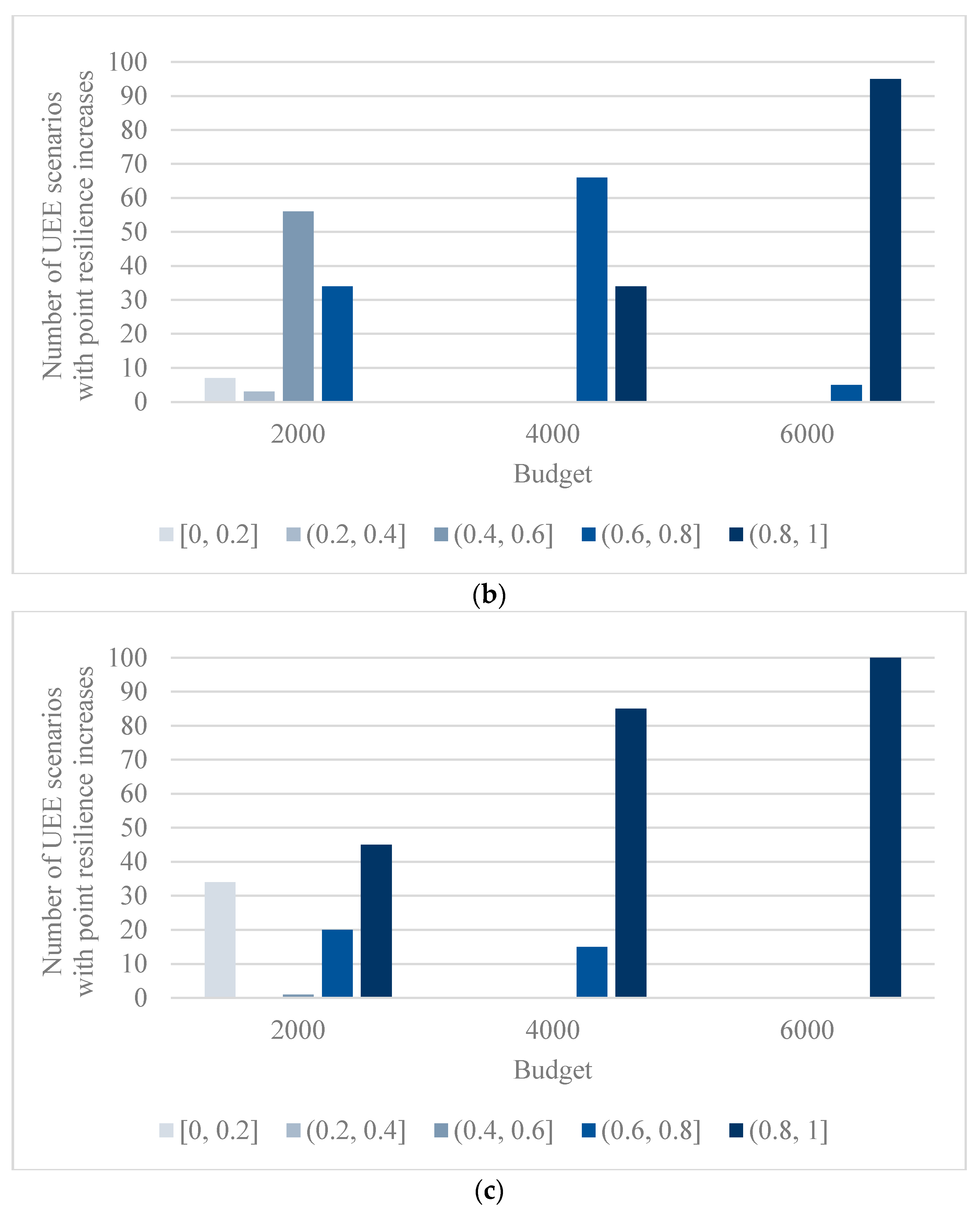
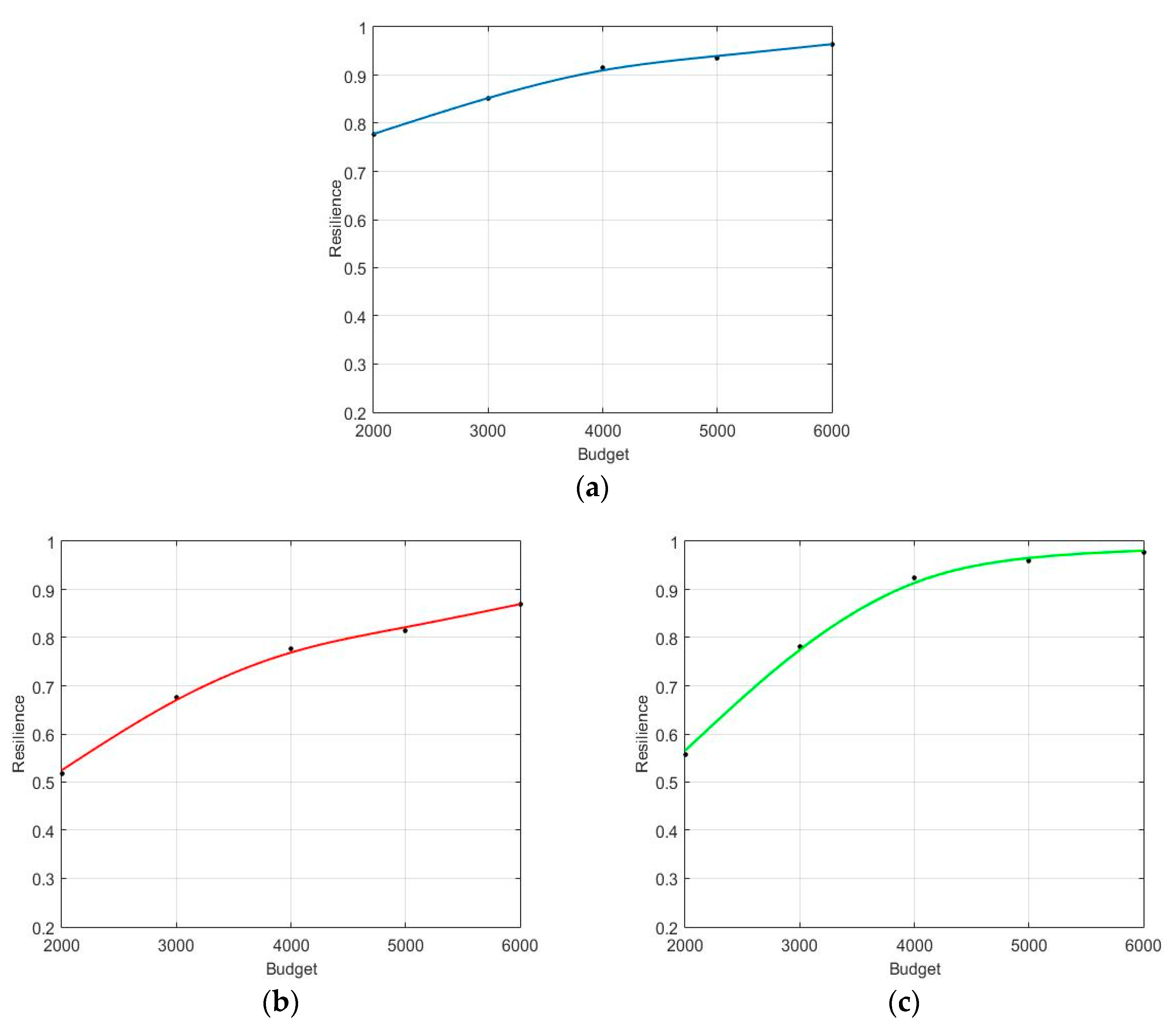
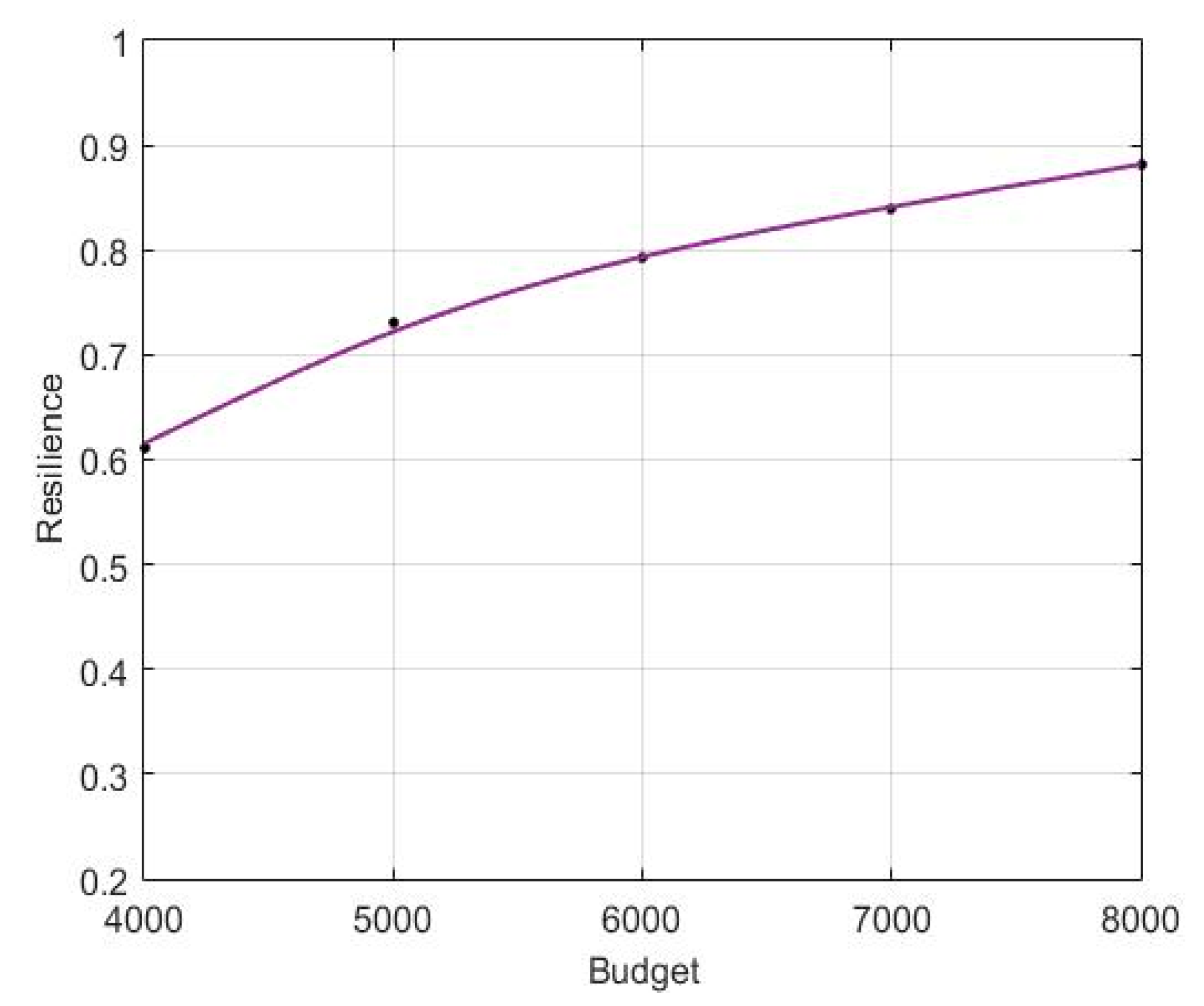
5.3. Analysis of the Influence of Maximum Budget for Recovery Activities
5.4. Comparison between the Lower Level SO and UE Models
- (1)
- PHCLTS user behaviors will influence the recovery decisions of the government, thereby affecting the point resilience of the test PHCLTS. In UEE scenario 1, the recovery decisions of the government are different in the lower level SO and UE models. In UEE scenario 2, the recovery decisions of the government are the same in the lower level SO and UE models, but the freight volume decisions made by the truck carriers are different, which lead to a different point resilience of the test PHCLTS.
- (2)
- The point resilience of the test PHCLTS with lower level SO and UE models has no absolute advantage. For each UEE type, most of the point resilience of the test PHCLTS with the lower level UE model is higher (Table 10).
- (3)
- For all UEE scenarios, the total transportation time with the lower level SO model is less than or equal to the corresponding value with the lower level UE model (Table 10). This result shows that the truck carriers that cooperate fully to reach an SO assignment perform better in transportation time consumption than those that make decisions independently to reach a UE assignment when facing UEEs.
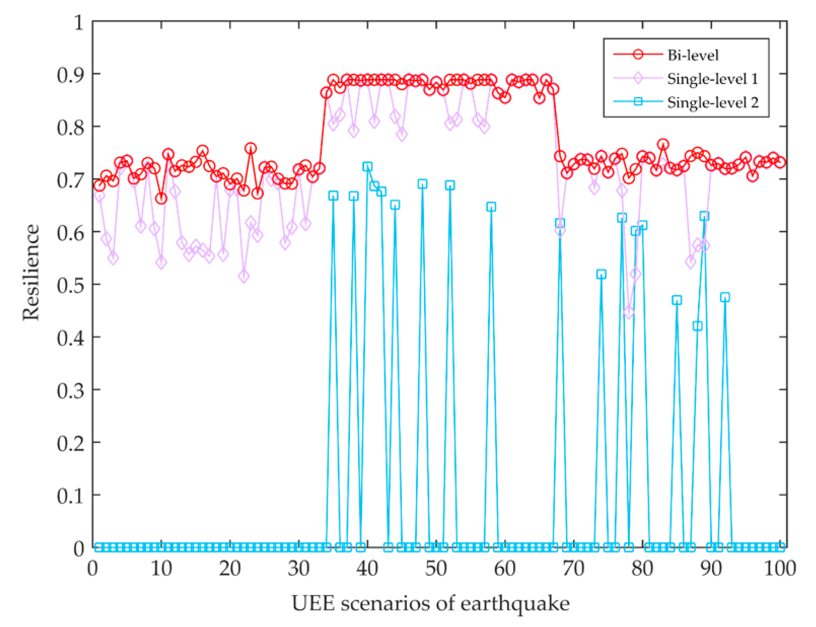
5.5. Comparison with Single-Level Programming Models
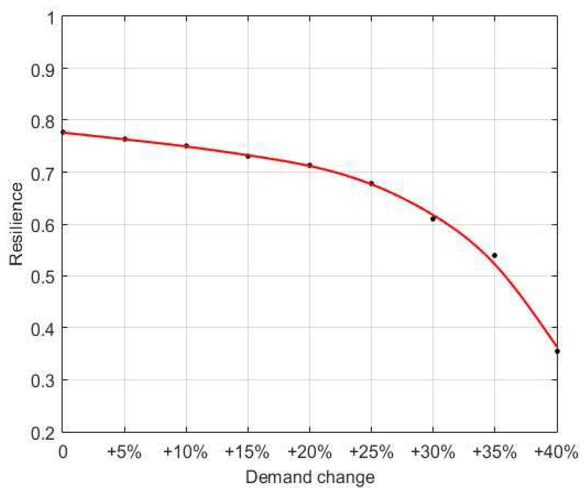
5.6. Analysis of the Influence of Demand in Hinterland Points
6. Managerial Insights and Conclusions
- (1)
- After the occurrence of UEEs, the implementation of appropriate recovery activities can effectively improve the resilience of PHCLTSs and reduce the negative influence caused by UEEs. When insufficient recovery activities are implemented, the resilience of PHCLTSs will be at a low level. Consequently, the total transportation time of containers will increase, and even the transportation demand in the hinterlands cannot be met, leading to negative effects on the economy and society. Appropriate recovery activities are crucial to reduce the negative effects after a UEE occurrence.
- (2)
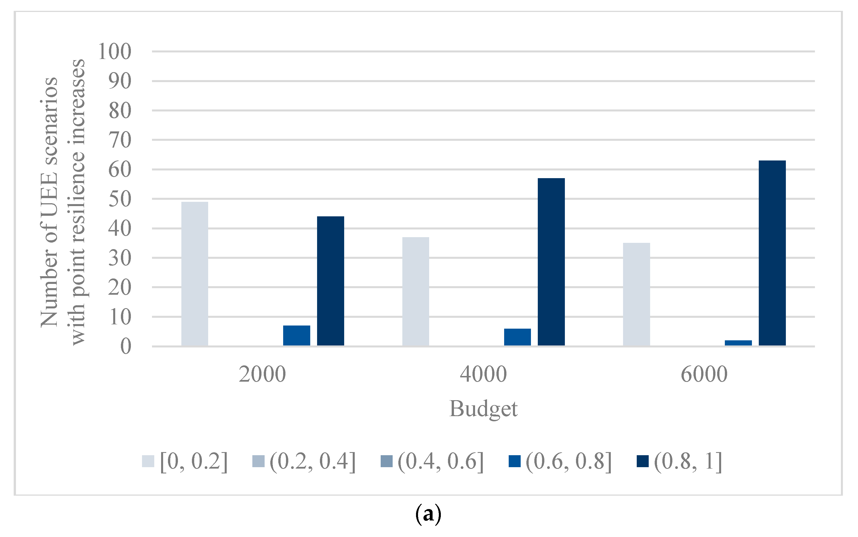
- The randomness of the negative effect on the test PHCLTS is gradually reduced as the budget increases. The resilience of PHCLTSs follows the law of diminishing returns. The government should prepare an appropriate budget in accordance with possible future UEE types.
- (3)
- PHCLTS user behaviors will influence the recovery decisions of the government, thereby affecting the resilience of PHCLTSs. Although facing the same UEE situation, the behavior patterns of PHCLTS users are different, and the government’s decision on the recovery activities also differs. The behaviors of PHCLTS users should be considered when studying this issue to improve the resilience of PHCLTSs.
- (4)
- From a long-term perspective, with the continuous growth in demand level, the resilience level of a PHCLTS shows a decreasing trend because the redundancy in the PHCLTS decreases. The government should adjust the recovery budget and the decisions on recovery activities in accordance with the changes in demand level to achieve a satisfactory resilience level of the PHCLTS.
- (5)
- The government should correctly predict the behaviors of PHCLTS users and their influence on the resilience of PHCLTSs when making decisions about recovery activities after UEEs. Otherwise, the resilience of PHCLTSs will be ineffectively improved, and resources will not be well utilized. The proposed bi-level programming models in this study can support the government in selecting a reasonable budget level and implementing efficient recovery decisions to improve the resilience of PHCLTSs in the face of UEEs.
Author Contributions
Funding
Institutional Review Board Statement
Informed Consent Statement
Data Availability Statement
Conflicts of Interest
Appendix A. Settings of Different UEE Types

| Detail a | |
|---|---|
| Subtype 1 of terrorist attack | 3 of 16 arcs in the PHCLTS are randomly chosen, and their capacity drops to 0. |
| Subtype 2 of terrorist attack | 4 of 16 arcs in the PHCLTS are randomly chosen, and their capacity drops to 0. |
| Subtype 3 of terrorist attack | 5 of 16 arcs in the PHCLTS are randomly chosen, and their capacity drops to 0. |
| Detail | |
|---|---|
| Subtype 1 of earthquake | Arc 9 is located at the epicenter, and the decrease percentage of its capacity is a uniform random number in the interval [0.9, 1]. Arcs 2, 5–8, 10–13 are affected by the earthquake, and the decrease percentages of their capacity are uniform random numbers in the interval [0.6, 0.8]. |
| Subtype 2 of earthquake | Arc 10 is located at the epicenter, and the decrease percentage of its capacity is a uniform random number in the interval [0.9, 1]. Arcs 6–8, 11–14 are affected by the earthquake, and the decrease percentages of their capacity are uniform random numbers in the interval [0.6, 0.8]. |
| Subtype 3 of earthquake | Arc 16 is located at the epicenter, and the decrease percentage of its capacity is a uniform random number in the interval [0.9, 1]. Arcs 6, 10–15 are affected by the earthquake, and the decrease percentages of their capacity are uniform random numbers in the interval [0.6, 0.8]. |
| Detail | |
|---|---|
| Subtype 1 of freeze | 1 warehouse in the PHCLTS is randomly chosen, and the decrease percentages of capacity of the arcs connected to this warehouse are uniform random numbers in the interval [0.7, 1]. |
| Subtype 2 of freeze | 2 adjacent warehouses in the PHCLTS are randomly chosen, and the decrease percentages of capacity of the arcs connected to these warehouses are uniform random numbers in the interval [0.7, 1]. |
| Subtype 3 of freeze | 3 adjacent warehouses in the PHCLTS are randomly chosen, and the decrease percentages of capacity of the arcs connected to these warehouses are uniform random numbers in the interval [0.7, 1]. |
Appendix B. Single-Level Programming Model 1
Appendix C. Single-Level Programming Model 2
References
- World Trade Organization. World Trade Report. 2019. Available online: https://www.wto.org/english/res_e/publications_e/wtr19_e.htm (accessed on 16 December 2020).
- Mansouri, M.; Sauser, B.; Boardman, J. Applications of systems thinking for resilience study in Maritime Transportation System of Systems. In Proceedings of the 3rd Annual IEEE International Systems Conference, Vancouver, BC, Canada, 23–26 March 2009; pp. 211–217. [Google Scholar]
- Chen, H.; Lam, J.S.L.; Liu, N. Strategic investment in enhancing port–hinterland container transportation network resilience: A network game theory approach. Transp. Res. Part B Methodol. 2018, 111, 83–112. [Google Scholar] [CrossRef]
- Chen, L.; Miller-Hooks, E. Resilience: An Indicator of Recovery Capability in Intermodal Freight Transport. Transp. Sci. 2012, 46, 109–123. [Google Scholar] [CrossRef]
- Ta, C.; Goodchild, A.V.; Pitera, K. Structuring a Definition of Resilience for the Freight Transportation System. Transp. Res. Rec. J. Transp. Res. Board 2009, 2097, 19–25. [Google Scholar] [CrossRef]
- Bard, J.F. Practical Bilevel Optimization: Algorithms and Applications; Kluwer Academic Publishers: Dordrecht, The Netherlands, 1998. [Google Scholar]
- Talley, W.K.; Ng, M. Hinterland transport chains: A behavioral examination approach. Transp. Res. Part E Logist. Transp. Rev. 2018, 113, 94–98. [Google Scholar] [CrossRef]
- Bruneau, M.; Chang, S.E.; Eguchi, R.T.; Lee, G.C.; O’Rourke, T.D.; Reinhorn, A.M.; Shinozuka, M.; Tierney, K.; Wallace, W.A.; Von Winterfeldt, D. A Framework to Quantitatively Assess and Enhance the Seismic Resilience of Communities. Earthq. Spectra 2003, 19, 733–752. [Google Scholar] [CrossRef] [Green Version]
- Murray-Tuite, P.M. A Comparison of Transportation Network Resilience under Simulated System Optimum and User Equilibrium Conditions. In Proceedings of the Winter Simulation Conference, Monterey, CA, USA, 3–6 December 2006. [Google Scholar]
- Omer, M.; Mostashari, A.; Nilchiani, R.; Mansouri, M. A framework for assessing resiliency of maritime transportation systems. Marit. Policy Manage. 2012, 39, 1–19. [Google Scholar] [CrossRef]
- Faturechi, R.; Miller-Hooks, E. Travel time resilience of roadway networks under disaster. Transp. Res. Part B Methodol. 2014, 70, 47–64. [Google Scholar] [CrossRef]
- Nair, R.; Avetisyan, H.; Miller-Hooks, E. Resilience Framework for Ports and Other Intermodal Components. Transp. Res. Rec. J. Transp. Res. Board 2010, 2166, 54–65. [Google Scholar] [CrossRef]
- Miller-Hooks, E.; Zhang, X.; Faturechi, R. Measuring and maximizing resilience of freight transportation networks. Comput. Oper. Res. 2012, 39, 1633–1643. [Google Scholar] [CrossRef]
- Chen, H.; Cullinane, K.; Liu, N. Developing a model for measuring the resilience of a port-hinterland container transportation network. Transp. Res. Part E Logist. Transp. Rev. 2017, 97, 282–301. [Google Scholar] [CrossRef]
- Friesz, T.L.; Harker, P.T. Freight network equilibrium: A review of the state of the art. In Analytical Studies in Transport Economics; Cambridge University Press: Cambridge, UK, 1985; pp. 161–206. [Google Scholar]
- Jones, D.A.; Farkas, J.L.; Bernstein, O.; Davis, C.E.; Turk, A.; Turnquist, M.A.; Nozick, L.K.; Levine, B.; Rawls, C.G.; Ostrowski, S.D.; et al. import/export container flow modeling and disruption analysis. Res. Transp. Econ. 2011, 32, 3–14. [Google Scholar] [CrossRef]
- Meng, Q.; Wang, X.C. Intermodal hub-and-spoke network design: Incorporating multiple stakeholders and multi-type containers. Transp. Res. Part B Methodol. 2011, 45, 724–742. [Google Scholar] [CrossRef]
- Corman, F.; Viti, F.; Negenborn, R.R. Equilibrium models in multimodal container transport systems. Flex. Serv. Manuf. J. 2017, 29, 125–153. [Google Scholar] [CrossRef] [Green Version]
- Zhang, B.; Yao, T.; Friesz, T.L.; Hongcheng, L. Urban Freight Transportation Planning: A Dynamic Stackelberg Game-Theoretic Approach. 2012. Available online: https://arxiv.org/abs/1211.3950 (accessed on 28 September 2019).
- Jiang, J.; Zhang, D.; Meng, Q.; Liu, Y. Regional multimodal logistics network design considering demand uncertainty and CO2 emission reduction target: A system-optimization approach. J. Clean. Prod. 2020, 248, 119304. [Google Scholar] [CrossRef]
- Yu, S.; Jiang, Y. Network design and delivery scheme optimisation under integrated air-rail freight transportation. Int. J. Logist. Res. Appl. 2021, 1–17. [Google Scholar] [CrossRef]
- Moreno-Quintero, E.; Fowkes, T.; Watling, D. Modelling Planner-Carrier Interactions in Road Freight Transport: Optimization of Road Maintenance Costs Via Overloading Control. Transp. Res. Part E Logist. Transp. Rev. 2013, 50, 68–83. [Google Scholar] [CrossRef] [Green Version]
- Lee, H.; Song, Y.; Choo, S.; Chung, K.-Y.; Lee, K.-D. Bi-level optimization programming for the shipper-carrier network problem. Clust. Comput. 2014, 17, 805–816. [Google Scholar] [CrossRef]
- Qiu, R.; Xu, J.; Ke, R.; Zeng, Z.; Wang, Y. Carbon pricing initiatives-based bi-level pollution routing problem. Eur. J. Oper. Res. 2020, 286, 203–217. [Google Scholar] [CrossRef]
- Li, S.; Liang, Y.; Wang, Z.; Zhang, D. An Optimization Model of a Sustainable City Logistics Network Design Based on Goal Programming. Sustainability 2021, 13, 7418. [Google Scholar] [CrossRef]
- De Jong, G.; Gunn, H.; Walker, W. National and International Freight Transport Models: An Overview and Ideas for Future Development. Transp. Rev. 2004, 24, 103–124. [Google Scholar] [CrossRef] [Green Version]
- Sheffi, Y. Urban Transportation Networks: Equilibrium Analysis with Mathematical Programming Methods; Prentice-Hall, Inc.: Hoboken, NJ, USA, 1985. [Google Scholar]
- Grey, A. The generalised cost dilemma. Transportation 1978, 7, 261–280. [Google Scholar] [CrossRef]
- Jeroslow, R.G. The polynomial hierarchy and a simple model for competitive analysis. Math. Program. 1985, 32, 146–164. [Google Scholar] [CrossRef]
- Assadipour, G.; Ke, G.Y.; Verma, M. A toll-based bi-level programming approach to managing hazardous materials shipments over an intermodal transportation network. Transp. Res. Part D Transp. Environ. 2016, 47, 208–221. [Google Scholar] [CrossRef]
- Soares, I.; Alves, M.J.; Antunes, C.H. Designing time-of-use tariffs in electricity retail markets using a bi-level model–Estimating bounds when the lower level problem cannot be exactly solved. Omega 2020, 93, 102027. [Google Scholar] [CrossRef]
- Zhang, S.; Chen, N.; She, N.; Li, K. Location optimization of a competitive distribution center for urban cold chain logistics in terms of low-carbon emissions. Comput. Ind. Eng. 2021, 154, 107120. [Google Scholar] [CrossRef]
- Kennedy, J.; Eberhart, R. Particle Swarm Optimization. In Proceedings of the ICNN’95-International Conference on Neural Networks, Perth, WA, Australia, 27 November–1 December 1995; pp. 1942–1948. [Google Scholar]
- Shi, Y. A Modified Particle Swarm Optimizer. In Proceedings of the IEEE Icec Conference, Anchorage, AK, USA, 4–9 May 1998. [Google Scholar]
- Zhao, Z.; Gu, X.; Li, T. Particle Swarm Optimization for Bi-level Programming Problem. Syst. Eng. Theory Pract. 2007, 27, 92–98. (In Chinese) [Google Scholar]
- Holmström, K.; Göran, A.O.; Edvall, M.M. User’s Guide for TOMLAB/CONOPT. 2007. Available online: https://tomopt.com/tomlab/products/conopt/ (accessed on 1 March 2021).
- Boyd, S.; Vandenberghe, L. Convex Optimization; Cambridge University Press: Cambridge, UK, 2004. [Google Scholar]
- López, L.F.M.; Blas, N.G.; Albert, A.A. Multidimensional knapsack problem optimization using a binary particle swarm model with genetic operations. Soft Comput. 2018, 22, 2567–2582. [Google Scholar] [CrossRef]
- Alves, M.J.; Antunes, C.H.; Carrasqueira, P. A Hybrid Genetic Algorithm for the Interaction of Electricity Retailers with Demand Response. In Applications of Evolutionary Computation 2016; Squillero, G., Burelli, P., Eds.; Springer: Berlin/Heidelberg, Germany, 2016; pp. 459–474. [Google Scholar]

| Notations | Meaning |
|---|---|
| Sets | |
| W | |
| K | Set of roadway intersections, i.e., set of nodes in a PHCLTS, except for the port and warehouses in hinterland, |
| A | |
| Aw | Set of arcs connected to warehouse w, Aw ⊆ A |
| Au | Set of arcs affected by UEEs, Au ⊆ A |
| Anu | Set of arcs unaffected by UEEs, Anu ⊆ A |
| U | |
| Indices | |
| sp | A port; only one port exists in a PHCLTS |
| w | A warehouse in hinterland, which represents the demand area |
| k | A roadway intersection |
| a | An arc, which represents one road of the PHCLTS. a(sp, k1) denotes an arc with origin sp and destination k1 |
| A UEE scenario | |
| Deterministic parameters | |
| Total transportation time of the PHCLTS in each transportation period pre-disaster | |
| Freight volume on arc a pre-disaster | |
| Transportation time on arc a pre-disaster | |
| ba | Cost of recovering 100% of the original capacity on arc a post-disaster. If the capacity of arc a recovered is , the recovery cost on arc a will be . |
| B | Maximum budget for recovery activities |
| Original transportation capacity of arc a | |
| Free-flow travel time on arc a pre-disaster, which is the transportation time on arc a without road impedance | |
| chu | Influence parameter of UEE type u on the free-flow travel time of arcs |
| Total generalized transportation costs of truck carriers in each transportation period pre-disaster. refers to the total generalized transportation costs pre-disaster following the SO principle; denotes the total generalized transportation costs pre-disaster following the UE principle | |
| ra | Transportation cost on arc a |
| q | Value of time |
| α and β | Parameters of “Bureau of Public Roads function”, which capture the influence of freight flow on transportation time of arc a |
| Dw | Daily transportation demand for warehouse w |
| UEE related variables (under UEE scenario ξ) | |
| Total transportation time of the PHCLTS in each transportation period post-disaster and after recovery | |
| Transportation time on arc a post-disaster and after recovery | |
| Capacity of arc a post-disaster and before recovery | |
| Capacity of arc a post-disaster and after recovery | |
| Free-flow travel time on arc a post-disaster and after recovery | |
| Total generalized transportation costs of truck carriers in each transportation period post-disaster and after recovery. refers to the total generalized transportation costs post-disaster and after recovery following the SO principle; denotes the total generalized transportation costs post-disaster and after recovery following the UE principle | |
| Decision variables | |
| In the upper level model | |
| Recovery levels of damaged capacity that the government implements on arc a under UEE scenario (: la = 1 means that the capacity of arc a is recovered to its original capacity, and la = 0 means that no recovery activity is implemented on arc a) | |
| In the lower level model | |
| Freight volume on arc a post-disaster and after recovery under UEE scenario ξ | |
| Notations | Meaning |
|---|---|
| n | Swarm size, i.e., the number of particles |
| Pi | |
| vi | |
| pbest | Particle’s best position |
| gbest | Whole swarm’s best position |
| c1 and c2 | Learning factors |
| r1 and r2 | Uniform random numbers in the interval [0, 1] |
| w | Inertia weight |
| wMax | Maximum inertia weight |
| wMin | Minimum inertia weight |
| iter | Number of iterations |
| iterMax | Maximum number of iterations |
| Tolerance |
| Value of Fitness Function | |||
|---|---|---|---|
| (Pi, Hi)/(Pj, Hj) whether or not to be a feasible solution of the bi-level programming model | Feasible/Feasible | (Pi, Hi) is better | (Pj, Hj) is better |
| Feasible/Infeasible | (Pi, Hi) is better | (Pi, Hi) is better | |
| Infeasible/Feasible | (Pj, Hj) is better | (Pj, Hj) is better | |
| Infeasible/Infeasible | (Pi, Hi) is better | (Pj, Hj) is better | |
| Arc ID | Origin | Destination | ra | ba | ||
|---|---|---|---|---|---|---|
| 1 | Port | Warehouse 1 | 1200 | 11 | 150 | 2400 |
| 2 | Port | Node 1 | 1600 | 5 | 60 | 3200 |
| 3 | Node 1 | Warehouse 1 | 600 | 6 | 80 | 1200 |
| 4 | Node 1 | Warehouse 2 | 1000 | 5 | 70 | 2000 |
| 5 | Node 1 | Warehouse 3 | 900 | 6 | 60 | 1800 |
| 6 | Port | Node 2 | 2400 | 5 | 60 | 4800 |
| 7 | Node 2 | Warehouse 1 | 900 | 7 | 70 | 1800 |
| 8 | Node 2 | Warehouse 2 | 600 | 6 | 60 | 1200 |
| 9 | Node 2 | Warehouse 3 | 600 | 5 | 70 | 1200 |
| 10 | Node 2 | Warehouse 4 | 600 | 6 | 60 | 1200 |
| 11 | Node 2 | Warehouse 5 | 800 | 7 | 80 | 1600 |
| 12 | Port | Node 3 | 1800 | 6 | 40 | 3600 |
| 13 | Node 3 | Warehouse 3 | 1000 | 6 | 70 | 2000 |
| 14 | Node 3 | Warehouse 4 | 1000 | 5 | 80 | 2000 |
| 15 | Node 3 | Warehouse 5 | 800 | 7 | 90 | 1600 |
| 16 | Port | Warehouse 5 | 1300 | 13 | 140 | 2600 |
| UEE Type | Detail |
|---|---|
| Terrorist attack | Some arcs in the PHCLTS are randomly chosen, and their capacity drops to 0. |
| Earthquake | An area is randomly chosen, and the capacity of the arcs in this area decreases. |
| Freeze a | Some nodes are randomly chosen, and the capacity of the arcs connected to these nodes decreases. |
| Resilience Level (Average Total Transportation Time) | |||
|---|---|---|---|
| Terrorist Attack | Earthquake | Freeze | |
| Lower level model 1—SO | 0.9164 (54,213) | 0.7761 (65,514) | 0.9244 (55,162) |
| Lower level model 2—UE | 0.9174 (54,635) | 0.7787 (65,921) | 0.9249 (55,652) |
| Budget | Recovery Levels of Damaged Arc Capacity | TOTAL Transportation Time | Point Resilience | |||
|---|---|---|---|---|---|---|
| Arc 6 | Arc 14 | Arc 16 | ||||
| With recovery activities | 6000 | 1.00 | 0.60 | 0 | 53,741 | 0.9370 |
| 4000 | 0.83 | 0 | 0 | 58,044 | 0.8676 | |
| 2000 | 0.42 | 0 | 0 | 68,564 | 0.7345 | |
| Without recovery activity | - | - | - | - | - | 0 |
| Recovery Budget | |||||
|---|---|---|---|---|---|
| 2000 | 3000 | 4000 | 5000 | 6000 | |
| Terrorist attack | 0.1027 | 0.0665 | 0.0221 | 0.0206 | 0.0027 |
| Earthquake | 0.0374 | 0.0075 | 0.0062 | 0.0038 | 0.0017 |
| Freeze | 0.1722 | 0.0987 | 0.0091 | 0.0029 | 0.0012 |
| Lower Level Model | Recovery Levels of Damaged Arc Capacity a (Decision of the Government) | Freight Volume on Each Arc (Decisions of the Truck Carriers) | Total Transportation Time (Upper Level) | Point Resilience | Total Generalized Costs (Lower Level) | |||||||
|---|---|---|---|---|---|---|---|---|---|---|---|---|
| UEE scenario 1 | SO model | Arc 1 | Arc 2 | Arc 3 | Arc 4 | Arc 1 | Arc 2 | Arc 3 | Arc 4 | 52,518 | 0.9589 | 1,058,137 |
| 1 | - | - | - | 512 | 1001 | 208 | 328 | |||||
| Arc 5 | Arc 6 | Arc 7 | Arc 8 | Arc 5 | Arc 6 | Arc 7 | Arc 8 | |||||
| - | - | - | - | 465 | 1516 | 280 | 172 | |||||
| Arc 9 | Arc 10 | Arc 11 | Arc 12 | Arc 9 | Arc 10 | Arc 11 | Arc 12 | |||||
| - | - | - | - | 335 | 243 | 486 | 257 | |||||
| Arc 13 | Arc 14 | Arc 15 | Arc 16 | Arc 13 | Arc 14 | Arc 15 | Arc 16 | |||||
| 0 | 0.8 | 0 | - | 0 | 257 | 0 | 714 | |||||
| UE model | Arc 1 | Arc 2 | Arc 3 | Arc 4 | Arc 1 | Arc 2 | Arc 3 | Arc 4 | 53,126 | 0.9565 | 1,051,428 | |
| 0 | - | - | - | 0 | 1133 | 404 | 287 | |||||
| Arc 5 | Arc 6 | Arc 7 | Arc 8 | Arc 5 | Arc 6 | Arc 7 | Arc 8 | |||||
| - | - | - | - | 442 | 1580 | 595 | 213 | |||||
| Arc 9 | Arc 10 | Arc 11 | Arc 12 | Arc 9 | Arc 10 | Arc 11 | Arc 12 | |||||
| - | - | - | - | 358 | 76 | 338 | 858 | |||||
| Arc 13 | Arc 14 | Arc 15 | Arc 16 | Arc 13 | Arc 14 | Arc 15 | Arc 16 | |||||
| 0 | 1 | 1 | - | 0 | 425 | 433 | 429 | |||||
| UEE scenario 2 | SO model | Arc 1 | Arc 2 | Arc 3 | Arc 4 | Arc 1 | Arc 2 | Arc 3 | Arc 4 | 56,674 | 0.8886 | 1,098,601 |
| - | - | - | - | 780 | 1520 | 220 | 500 | |||||
| Arc 5 | Arc 6 | Arc 7 | Arc 8 | Arc 5 | Arc 6 | Arc 7 | Arc 8 | |||||
| - | 0 | 0 | 0 | 800 | 0 | 0 | 0 | |||||
| Arc 9 | Arc 10 | Arc 11 | Arc 12 | Arc 9 | Arc 10 | Arc 11 | Arc 12 | |||||
| 0 | 0 | 0 | 1 | 0 | 0 | 0 | 994 | |||||
| Arc 13 | Arc 14 | Arc 15 | Arc 16 | Arc 13 | Arc 14 | Arc 15 | Arc 16 | |||||
| 0 | 1 | - | - | 0 | 500 | 494 | 706 | |||||
| UE model | Arc 1 | Arc 2 | Arc 3 | Arc 4 | Arc 1 | Arc 2 | Arc 3 | Arc 4 | 56,881 | 0.8933 | 1,099,634 | |
| - | - | - | - | 728 | 1572 | 272 | 500 | |||||
| Arc 5 | Arc 6 | Arc 7 | Arc 8 | Arc 5 | Arc 6 | Arc 7 | Arc 8 | |||||
| - | 0 | 0 | 0 | 800 | 0 | 0 | 0 | |||||
| Arc 9 | Arc 10 | Arc 11 | Arc 12 | Arc 9 | Arc 10 | Arc 11 | Arc 12 | |||||
| 0 | 0 | 0 | 1 | 0 | 0 | 0 | 1046 | |||||
| Arc 13 | Arc 14 | Arc 15 | Arc 16 | Arc 13 | Arc 14 | Arc 15 | Arc 16 | |||||
| 0 | 1 | - | - | 0 | 500 | 546 | 654 | |||||
| Higher Point Resilience | Equal Point Resilience | Lower Total Transportation Time | Equal Total Transportation Time | |||
|---|---|---|---|---|---|---|
| Lower Level SO Model | Lower Level UE Model | Lower Level SO Model | Lower Level UE Model | |||
| Terrorist attack a | 22% | 76% | 0 | 96% | 0 | 2% |
| Earthquake | 11% | 89% | 0 | 100% | 0 | 0 |
| Freeze | 9% | 79% | 12% b | 100% | 0 | 0 |
| Recovery Levels of Damaged Arc Capacity a (Decision of the Government) | Freight Volume on Each Arc (Decisions of the Truck Carriers) | Total Transportation Time (Upper Level) | Point Resilience | |||||||
|---|---|---|---|---|---|---|---|---|---|---|
| Bi-level programming model | Arc 1 | Arc 2 | Arc 3 | Arc 4 | Arc 1 | Arc 2 | Arc 3 | Arc 4 | 67,147 | 0.7500 |
| - | - | - | - | 780 | 1520 | 220 | 500 | |||
| Arc 5 | Arc 6 | Arc 7 | Arc 8 | Arc 5 | Arc 6 | Arc 7 | Arc 8 | |||
| - | 0.29 | - | - | 800 | 500 | 0 | 0 | |||
| Arc 9 | Arc 10 | Arc 11 | Arc 12 | Arc 9 | Arc 10 | Arc 11 | Arc 12 | |||
| - | 1 | 0 | 0 | 0 | 500 | 0 | 0 | |||
| Arc 13 | Arc 14 | Arc 15 | Arc 16 | Arc 13 | Arc 14 | Arc 15 | Arc 16 | |||
| 0 | 0 | 0 | 1 | 0 | 0 | 0 | 1200 | |||
| Single-level programming model 1 | Arc 1 | Arc 2 | Arc 3 | Arc 4 | Arc 1 | Arc 2 | Arc 3 | Arc 4 | 87,636 | 0.5746 |
| - | - | - | - | 780 | 1520 | 220 | 500 | |||
| Arc 5 | Arc 6 | Arc 7 | Arc 8 | Arc 5 | Arc 6 | Arc 7 | Arc 8 | |||
| - | 0.47 | - | - | 800 | 1300 | 0 | 0 | |||
| Arc 9 | Arc 10 | Arc 11 | Arc 12 | Arc 9 | Arc 10 | Arc 11 | Arc 12 | |||
| - | 1 | 1 | 1 | 0 | 500 | 800 | 400 | |||
| Arc 13 | Arc 14 | Arc 15 | Arc 16 | Arc 13 | Arc 14 | Arc 15 | Arc 16 | |||
| 0 | 0 | 0 | 0.72 | 0 | 0 | 400 | 0 | |||
| Single-level programming model 2 | Arc 1 | Arc 2 | Arc 3 | Arc 4 | Arc 1 | Arc 2 | Arc 3 | Arc 4 | 119,700 | 0.4207 |
| - | - | - | - | 731 | 1346 | 269 | 500 | |||
| Arc 5 | Arc 6 | Arc 7 | Arc 8 | Arc 5 | Arc 6 | Arc 7 | Arc 8 | |||
| - | 0.64 | - | - | 577 | 750 | 0 | 0 | |||
| Arc 9 | Arc 10 | Arc 11 | Arc 12 | Arc 9 | Arc 10 | Arc 11 | Arc 12 | |||
| - | 0 | 0 | 0.24 | 223 | 230 | 297 | 379 | |||
| Arc 13 | Arc 14 | Arc 15 | Arc 16 | Arc 13 | Arc 14 | Arc 15 | Arc 16 | |||
| 0 | 0 | 0 | 0.63 | 0 | 270 | 109 | 794 | |||
Publisher’s Note: MDPI stays neutral with regard to jurisdictional claims in published maps and institutional affiliations. |
© 2021 by the authors. Licensee MDPI, Basel, Switzerland. This article is an open access article distributed under the terms and conditions of the Creative Commons Attribution (CC BY) license (https://creativecommons.org/licenses/by/4.0/).
Share and Cite
Gao, S.; Liu, N. Improving the Resilience of Port–Hinterland Container Logistics Transportation Systems: A Bi-Level Programming Approach. Sustainability 2022, 14, 180. https://doi.org/10.3390/su14010180
Gao S, Liu N. Improving the Resilience of Port–Hinterland Container Logistics Transportation Systems: A Bi-Level Programming Approach. Sustainability. 2022; 14(1):180. https://doi.org/10.3390/su14010180
Chicago/Turabian StyleGao, Song, and Nan Liu. 2022. "Improving the Resilience of Port–Hinterland Container Logistics Transportation Systems: A Bi-Level Programming Approach" Sustainability 14, no. 1: 180. https://doi.org/10.3390/su14010180
APA StyleGao, S., & Liu, N. (2022). Improving the Resilience of Port–Hinterland Container Logistics Transportation Systems: A Bi-Level Programming Approach. Sustainability, 14(1), 180. https://doi.org/10.3390/su14010180