1. Introduction
The critical dependence of today’s society on a secure supply of energy is well known. The heightening worries for the accessibility of primary energy and the ever mellowing infrastructure of the present transmission and distribution (T&D) networks pose a continuous threat to security, reliability and standard of power supplied. Conventional generation sources (CGSs) like diesel and natural gas–based generation plants steadily add to greenhouse gas emissions (GHGs) resulting in increased global warming and sudden climate changes. Hence, the generating capacity of CGSs to meet the growing global demand for energy is severely limited. This has given a massive push to alternatives called as renewable energy sources (RES) which include energy from solar, wind and biomass sources. The setup of RES integrated in a distribution system is commonly referred to as distributed generation (DG). DG is typically installed at medium voltage (MV) and high voltage (HV) levels and power flow is uni-directional keeping in mind the passive nature of consumer loads. Due to this, extensive research has been carried out on the linkage of DG within distribution networks. This includes topics stretching from control and protection of DG integrated distribution networks to the quality of power supplied by them. A number of RES including photovoltaics (PV), wind energy conversion systems (WECS), micro-turbines (MT) and fuel cells (FC) have come up as encouraging alternatives to meet the ever increasing load demands without compromising on power quality besides addressing different economic and environmental concerns. Out of different RES, solar PV systems and WECS are the most utilised ones owing to their high energy potential and easy availability [
1]. DG has led to massive improvement in power quality besides engineering a remarkable decrease in T&D losses by meeting the load demands locally. Furthermore, it has improved service quality by decreasing the distance between load and point of generation.
The most efficient way to meet the growing energy needs is to include novel technologies in DG systems and grid architectures. Power electronic converters (PECs) interfaced with DGs have led to tenable structures called (MGs) [
2,
3,
4,
5,
6]. A MG is defined as a network that can inventively combine the activities of all entities linked to it—generators, consumers and loads to competently provide tenable, profitable and fixed power supply. It utilizes intelligent monitoring, control and communication technologies to achieve these objectives. Until very recently, AC MG used to be the main electrical architecture for supplying power to remote and inaccessible networks [
5,
7,
8]. Eventually, it has been replaced by the concept of a DC MG owing to increased use of DC loads over the years and also due to the fact that DC power is generated by a bulk of DG sources. The major benefits of a DC MG include absence of AC-DC or DC-AC conversion stages leading to increased efficiency and reliability [
9,
10,
11,
12,
13]. However, AC MGs are still presiding due to the use of AC based DG and loads. An AC MG can also be directly linked with the traditional distribution systems with least adjustments. Hence, it is profitable to design a new architecture to merge these two types of MGs by means of a bidirectional interlinking converter (ILC) to extricate the advantages of both these categories [
14,
15,
16,
17]. This notion of merging DC and AC MGs is referred to as a hybrid MG. This type of architecture can accommodate both types of DG sources and loads to warrant trouble-free transfer of power between two sub-grids. It can operate in both grid connected and stand-alone modes while regulating power flow by means of the ILC. However, the stand-alone mode of a hybrid MG is relatively way more perilous due to demand-generation regulation and the intermittent nature of DG sources.
Power sharing in a hybrid MG is an emerging topic and has been extensively researched about in this decade. An AC MG employs active power-frequency and reactive power-frequency droop characteristics for power sharing while as current-voltage and active power-voltage droop characteristics are employed in a DC MG. As a result, control algorithms of both the individual MGs should be synchronised with the ILC to warrant supply of quality power to the end users. The control techniques of a MG are mainly categorised into three sections namely primary control, secondary control and tertiary control. The primary control stablises voltage and frequency without the need of communication links. The voltage and frequency deviations then are recompensed by the secondary controller which regulates power quality and energy management of MGs. It is further sub-categorised into centralized and decentralized control. In the former, a central controller optimises the control decisions by acquiring pertinent data from the network. In the latter, all DG sources operate in parallel to regulate energy management by employing the information acquired from neighboring sources. The tertiary control improves the power quality by regulating energy management between various MGs and the utility grid and it is administered by collaboration between a MG and the utility grid. The non-dispatchable and intermittent nature of electric power produced by DG sources requires a MG system for their trouble-free working and productive integration with the power system [
5,
17,
18,
19,
20]. Energy Storage Systems (ESS) and CGS are employed to address the sporadic nature of DG power [
21,
22]. However, ESS alone can’t alleviate the problem of balancing and keeping in mind the environmental constraints, alternative substitutes are required due to high GHG emissions of CGS. Demand response and prosumers are the finest alternatives unfolding that could assist in stabilising power demand locally [
23,
24]. This paper presents a review of AC/DC micro-grids and their architecture, their state-space modeling and power management aspects and their impact on a distribution system. This paper is organised as follows:
Section 2 introduces the architecture and classification of MGs,
Section 3,
Section 4 and
Section 5 discuss the state space modeling of different MG components,
Section 6 discusses MG protection,
Section 7 discusses the power management strategies of a hybrid MG in grid connected and stand-alone modes,
Section 8 presents the MG impact on a distribution network and finally, the review conclusions are summed up in
Section 9.
2. Microgrid and Its Architecture
Numerous definitions of MG have been put forward over the years taking into consideration various characteristics associated with its applications [
25,
26,
27,
28]. MG has been defined as “the idea of nomadic DG sources like PV, wind, storage devices and different loads in the prevailing power system which can be controlled either in grid-connected or in stand-alone modes” in [
25]. The authors in [
26] have explained MG as “a scaled-down power system which comprises DG sources, controllers and loads”. MGs consist of low voltage (LV) distribution systems and they work in grid-connected or stand-alone modes.
2.1. MG Architectures
Hybrid MGs work on the concept of both AC and DC power and their architectures are dictated by the character of loads, DG sources involved, the room to adjust ESS and their energy needs. MG architectures can be divided into three classes depending on architecture of the system and its voltage characteristics. These are AC MG, DC MG and hybrid MG [
29,
30,
31]. Additionally, MGs can be categorised as per their utilisation areas like utility MGs, institutional MGs, commercial and industrial MGs, transportation MGs and remote-area MGs [
32].
Figure 1 illustrates the classification of a MG into different categories. A flexible MG has to be able to import/ export energy from/to the grid, while controlling active and reactive-power flow by managing energy storage. Based on operating modes, MGs are categorised into grid-connected, transited, or island, and reconnection modes, which increase their reliability by disconnecting them from the grid in case of network failures. In terms of power or voltage characteristics, MGs are categorized into AC power system, DC power system, hybrid system networks or simply as AC, DC and hybrid MGs. In addition, MGs can be categorised based on their application areas like utility MGs, institutional MGs, commercial and industrial MGs, transportation MGs and remote-area MGs. In addition to this, campus MGs support multiple loads situated in a constrained geographical location, community MGs which support penetration of local energy and millitary base MGs which focus on physical and cyber security for military facilities. A tabular comparison of AC, DC and hybrid MGs is given in
Table 1.
2.2. Microgrid Toplogies
Different architectures are required to regulate the flow of energy from various sources into the utility grid. MGs are largely categorised into AC, DC and hybrid MGs.
2.2.1. AC Microgrids
This is the most traditional form of MG where PECs are employed to integrate DG sources with electrical networks [
33] and needs minimum modifications for its integration. These MGs are integrated with MV and LV distribution networks to increase power flow and decrease transmission line losses in distribution networks. Here, power moves directly from/to the grid sans any converter. The connected loads, DG sources and ESS must be grid-adaptable as the feeder voltage and frequency matches with the grid conditions. This gives rise to the main advantage of AC MGs which is their affinity with the conventional grid which can be recomposed to an AC MG strategy. However, the presence of complex PEC interfaces to synchronize DERs with the utility grid and to supply good quality AC currents which is devoid of harmonics presents one of the major drawbacks of AC MGs which reduces the efficiency and reliability of the system. Also, certain issues crop up upon their integration like system stability, power quality and shortage of reactive power. These are addressed by applying advanced control techniques [
34,
35]. The MG is able to adjust power generation and load demand to any working condition by switching its topology by means of circuit breakers. The inter-connection of the MG with the distribution grid is governed by the static switch. It can disengage the MG when the quality of power being supplied to the distribution grid is below par making it to operate in is-landed mode. At times of a grid fault, the static switch as well as the circuit breaker open to disengage the non-critical loads from the grid to elude their impairment [
36]. This sustains good quality and reliable power supply to delicate loads that are catered from DG sources and ESS.
2.2.2. DC Microgrids
A majority of the current consumer loads work on DC. Hence, their integration with DC MGs is a smart choice due to increased efficiency and power quality independence from the distribution grid. Around 35% of the generated AC power is fed to a PEC before its utilization [
37]. Majority of DC loads, DC-based DG sources and PECs are employed for varied applications due to the technological prowess of the latter [
38]. This has created a sea of new opportunities in the field of DC MGs due to reduced losses during power conversion and absence of reactive current circulation [
39,
40]. An AC/DC bi-directional interface called as the interlinking converter (IC) is the primary architect in a DC MG which links it to the AC grid after providing the necessary voltage shift and galvanic isolation. All DG sources and storage devices are linked with the DC bus via a PE interface (DC/DC or AC/DC).
DC MGs possess a plethora of advantages as there are relatively lower transmission losses owing to the non-existence of reactive current circulation. They possess simple architecture and control requirements as grid synchronization, harmonics and reactive power do not bother them. Additionally, they possess fault-ride-through ability and are least influenced by blackouts or voltage sags due to the presence of capacitors. However, they have their own shortcomings which include the need to construct DC distribution systems and the need to address their incompatibility with traditional electrical systems. Also, they face challenges in protection schemes due to immature guidelines and constrained practical involvements. As such, they need special protection mechanisms to address DC short-circuit current interruption due to the absence of zero-point crossing of the current waveform. Also, DC MGs need additional converters as they are not feasible for direct connection of AC loads. However, the biggest drawback of this architecture is the presence of series-connected IC which handles power flow with the utility grid as it decreases system reliability [
41].
2.2.3. Hybrid MGs
Hybrid MGs are a combination of AC and DC MGs and are gaining attention because they facilitate the direct integration of DGs, loads and storage devices with the traditional distribution system [
36,
42]. They possess the advantages of both MGs like increased reliability and efficient economic operation. Hybrid MGs cater to all types of loads and reduce inverter and rectifier power losses. However, they demand a robust coordinated control and increased investigation due to the intermittency of DG sources and reactive power compensation. Hybrid MGs are further classified as coupled and decoupled AC configurations on the basis of the interfacing device and the grid connection. The AC bus of the MG is directly integrated with the grid by means of a transformer and an AC/DC converter is employed for the DC link in the former while as the latter comprise an AC/DC and a DC/AC stage with no direct linkage between the grid and the bus.
Figure 2 depicts the architecture of a typical hybrid MG. It clearly distinguishes between the AC and DC grids and interlinks them by means of a bidirectional AC-DC converter [
36]. The AC bus caters to the AC loads while as the DC bus caters to the DC loads while as the DG sources and storage units are connected at either of the buses. A PE converter is employed for maintaining the necessary voltage levels. This architecture lets the installation of critical loads onto the DC feeder while as more robust loads are installed onto the AC feeder [
34,
36]. It decreases conversion phases and consequently the energy wastage. It is straightforward to limit harmonics into the AC side from the DC side thus improving the quality of power in the grid. Voltage transformations in the AC side can be carried out in a simple manner by means of conventional transformers while as DC-DC converters do the job in the DC side of the network. Although the initial investment of a hybrid MG is higher due to the inclusion of a principal AC-DC converter and a communication system for device interconnections, it is beneficial in the long run as it reduces the number of interfacing converters as number of attached devices increases. However, the DC side of a hybrid MG is still under study as far as protection problems of the MG are concerned. Also, the reliability of a hybrid MG takes a hit owing to the main interface PE converter. The power flow management is relatively complex because appropriate control strategies need to be applied for the connected devices to ensure a stable and reliable power flow. Power balance between the AC and DC side of a hybrid MG is a major challenge and it is still under study.
3. State Space Representation of PV Model
A MG integrates large number of DG sources into power system to provide greater reliability and continuity to critical loads. The dynamic properties of various RES like PV and wind and their inverter controls need to be integrated as state space models to increase system accuracy. This is necessitated due to the intermittency of solar and wind power and various disturbances in the power system. This section presents a state space model for MG components comprising double stage PV systems, WECS and mathematical model of parallel inverters explicitly in equations considering system dynamics and control functions.
Regarding the power circuit modeling of PV arrays, most of the literature considers simplified models [
43,
44,
45,
46,
47,
48,
49] only in continuous conduction mode (CCM) for the dc/dc converter [
50,
51,
52]. However, discontinuous conduction mode (DCM) is frequently noticed at lower power intensities arising due to less irradiance and faulty conditions which conclusively changes the system dynamics. This paper discusses the need of both CCM and DCM modes in PV models. PV control is of extreme significance for dynamic system evaluations [
49,
53]. The classic control strategy of a double-stage PV system includes: (a) a maximum power point tracking (MPPT) algorithm for the converter, (b) a PI controller dedicated for the DC-link capacitor, (c) decoupled inverter control (current) and (d) a phase locked loop (PLL) structure to track grid voltage. The dynamics of MPPT is abandoned in some literature [
54] which presumes that the system operates at MPP at all times and ensues an erroneous reaction to sudden changes in irradiance [
49,
51]. Another key feature includes a detailed dynamic model formulation. Most of the above mentioned literature depicts models employing an amalgamation of system block diagrams, differential equations and flowcharts. Only a small number of models are presented completely in the rigorous state-space form which encompasses an extensive range of applications. This review specifies that all the mentioned dynamic PV models till date are designed for particular applications and there is plenty of room to develop a generic relevant solution which addresses all the contemporary demands. The purpose of this work is to obtain a dynamic double stage PV model that subdues these constraints and presents a state-of-the-art generic PV dynamic model applicable in all circumstances. This model is composed in state-space form and it considers the DC-side dynamics and appropriates a non-simplified single-diode PV model and covers both CCM and DCM operations of the boost converter (BC). The control strategy comprises MPPT control, DC link control, reactive power control aided with suitable PLL mechanism. The electric circuit and control strategy of a double stage PV system is depicted in
Figure 1.
The electric circuit comprises a PV cell, BC, DC link capacitor, inverter and filter. The control arrangement consists of MPPT control and curtail control for the BC and DC link control, reactive power control and current control subsystem for the inverter. The state-space representation of the overall PV system consists of 20 state variables together with a combination of differential and algebraic equations:
where
x represents the state vector,
v represents the input vector and
y represents the output vector. Mathematically,
3.1. System Description
3.1.1. PV Generator
The PV array model is generated with the help of the well known single-diode PV model. It is governed by five variables namely
,
,
a,
and
. The algebraic equation involving the dynamics of the PV system [
51] is difficult to solve and involves a lot of computational intricacies. However, the use of ‘lambert W’ function eases and modifies the equation [
55,
56] which is given as:
where
and
are PV and saturation currents, respectively and
=
represents thermal voltage of the array with
series cells.
and
represent equivalent series and shunt resistance of the array. ‘
k’ represents the Boltzmann constant, ‘
T’ represents
p–
n junction temperature and ‘
a’ is the diode ideality constant. The Lambert
W function is computed by means of the built-in
lambertw MATLAB function.
This equation expresses
explicitly as a function of
. The parameters of Equation (
5) are calculated by extracting the reference variables [
57]
,
,
,
and
.
3.1.2. Boost Converter
The BC of a double-stage PV system [
45,
46,
51] is designated by the ensuing equations by taking into consideration the average models:
where
represents inductor current,
represents DC link voltage,
D is the duty cycle and
represent the circuit parameters and
represents the complete time of conduction of the inductor for period
.
during continuous conduction mode.
The inductor’s continuous conduction mode current is calculated by putting
= 0 and is given as
The inductor’s discontinuous conduction mode current is calculated as
The current in the inductor is the highest of the following two values:
3.1.3. DC Link Capacitor
The general equation for a DC link model that counts for both the conduction modes [
45,
46] is given as:
where
represents DC link capacitance and
represent inverter voltages and currents in
d-
q frame.
3.1.4. Filter
The state-space model of the interfacing inductance is given as [
45,
47,
54,
58]:
where
represent inverter voltages,
represent grid voltages and
represent inverter currents in the
d-
q frame rotating at synchronous speed
.
represent parameters of the filter.
4. Solar PV Control Model
This section explains the typical control scheme for enhancing the frequency response of the system.
4.1. Boost Converter Control
Traditionally, the control of a BC entails an MPPT algorithm to draw peak power all the time. However, the PV system should be adept at decreasing power output during contingencies. Usually, this is achieved by regulating the voltage of the PV system to sub-optimal levels during times of power curtailment [
59,
60]. The control strategy depicted in
Figure 3 executes this task. It comprises two control modules viz; the MPPT control and curtail control which are activated or deactivated in line with the operating mode.
4.1.1. MPPT Control
Different algorithms like Perturb & Observe (P&O), Incemental Conductance (INC) are used during MPPT control to establish the optimal reference PV voltage. The state space representation [
51] employs reference voltage, PV voltage and PV power as state variables and is given as:
where ‘
k’ represents discrete time instant. The sign function yields ± 1 as per the sign of the argument and the time-step equals 1 when the converter is in MPP mode. Else, it returns 0.
The duty cycle
D is regulated by the PI controller to adjust the actual and reference PV voltages,
and
. The duty cycle
D is contained between 0 and 1 by the following equations using the state variable
.
where
represent controller gains and
sat represents saturation within range.
4.1.2. Curtail Control
Curtail mode pauses the MPPT operation by making reference voltage constant and activates curtail control mode in which a PI controller makes a voltage adaptation
to adjust PV power
with the setpoint value
.
where
represents the state variable and
,
represent the gains of the controller. The set-point power
is given by:
Here denotes the peak obtainable PV power and , , , ‘eff’ indicate the frequency-response power adaptation, the needed reserve power, apparent power limit of the inverter and the converter efficiency, respectively.
4.2. Inverter Control
The inverter control arrangement comprises DC link control, reactive power control and current control to address unbalanced operation of grid and the urgent need for injection of reactive currents.While the former is mentioned here, the latter has not found a mention due to its extensive reference in the literature [
54,
61].
DC Link Control
The DC link controller compares DC link voltage with the reference voltage and maintains it at a constant value and regulates the quantity of power transferred to the grid. Initially,
is calculated from the sensed voltage by filtering it from 100 Hz oscillations occurring due to asymmetrical faults [
50].
where
represent state variables and
is the quality factor.
The reference power
is exported under a higher limit
to limit flow of active power during faults. The reference power input to the PI controller is calculated as:
where
and
represent controller gains.
5. Modeling of Wind Energy Conversion Systems
The application of wind energy has grown markedly over the years and its significance in its integration with power system has assumed tremendous importance [
62]. Several studies have carried out extensive analysis of a design of wind farm [
63,
64]. This includes the effect of wind generation with regard to power flow, voltage profile, flow of short-circuit currents, reactive power ability and transient stability [
65,
66]. Different wind turbine models have been described in the literature as per their application. A comprehensive depiction of separate units and their inter-connection with the system is considered at times. On the other hand, wind farms may be modeled as lumped equivalent machines as seen from the system [
65]. Nonetheless, the model response hangs on the kind of equipment being used. Numerous derived dynamic models find a mention in the literature [
67,
68,
69]. This section presents state-space modeling of synchronous and induction machines employed in wind energy conversion systems. Reduced order models can be derived directly from these models which can prove to be important tools in power system evaluations. These models are derived with multiple state variables employable in different control strategies for a convenient and compact assessment in terms of controllability and stability of wind energy conversion systems. The two common type of wind turbine configurations are fixed speed wind turbines and variable speed wind turbines. While the former are simple devices comprising a gearbox, shaft and a generator, the latter have evolved owing to the increased size of wind turbines [
67,
68,
70]. The state-space representation is acquired by assuming that
- (a)
If flowing inwards, the stator current is taken as negative.
- (b)
Synchronous reference frame is used to derive the equations.
- (c)
q-axis leads the d-axis by 90°.
The state space representation employed by all models is given as
5.1. System Description
The suggested system is depicted in
Figure 4 and represents a single WTS which comprises a variable-speed, variable-pitch, horizontal axis, lift turbine. The WTS may or may not comprise a gear between turbine and generator (PMSG in this case). The generator supplies power through a back-to-back converter and filter to the point of common coupling (PCC). The VSI operates in grid-feeding mode as the grid is presumed to be symmetrical.
5.1.1. Turbine Aerodynamics and Torque
The wind turbine translates wind energy into rotational energy. The wind power extracted is given as
where
is the air density,
r is the rotor radius and
is wind velocity. However, the power that can be extracted by the turbine is limited by the Betz limit and is given as
is a function of wind velocity
, angular velocity
, pitch-angle
and tip speed ratio
. The coefficient of power
is calculated by the following function
The constants are and ‘f’ is a continuously differentiable function.
5.1.2. Pitch Control System
The pitch control regulates the pitch angle
within range of its defined reference
. Its nonlinear dynamics are approximated by
where
=
and
and
represent peak workable change rate of pitch angle and time constant of pitch control system, respectively (see
Figure 5).
5.1.3. Turbine Torque
The turbine facilitates the conversion of wind energy into rotational energy. Turbine torque is computed from turbine power and turbine angular velocity as follows:
5.2. Electrical System in Three-Phase Reference Frame
In
Figure 6, the electrical network of the considered PMSG is shown. The network of the machine-side depicts the stator phase voltages
, stator phase current
, stator phase resistance
and stator flux linkage
. The grid-side network comprises filter and grid with filter phase voltages
, filter phase currents
, filter resistance
, filter inductance
and grid phase voltages
. Power is exchanged between converters via DC-link capacitor.
5.2.1. DC-Link Dynamics
The extensively utilised two-level back-to-back converters are considered for DC link dynamics of WECS. The VSC is modeled by employing ideal switches and is shown in
Figure 7.
refers to the generator phase voltages that are fed from the stator side while as
refers to phase voltages of the line filter generated by the filter-side converter. The converter output voltage is generated by appropriate modulation techniques with the help of switching vectors
and
. There are eight possible switching vectors for the considered two-level VSCs such that
. The stator and filter voltages are given as
The charging or discharging of DC-link capacitor is dependent upon the machine-side and grid-side currents (
Figure 6). The DC-link dynamics are calculated as
where
.
5.2.2. Grid Side Dynamics
This includes filter, PCC and grid. A line filter is employed to filter out switching ripples and induce sinusoidal phase currents in the grid. An RC filter and a filter inductance is considered for this purpose. The grid-side voltages
are applied to the filter which outputs sinusoidal filter phase currents
. The copper losses are dissipated in the filter resistance
, The grid-side electrical network of a WECS is depicted in
Figure 6. The grid-side dynamics are given by
where the term inside the short parentheses represents grid voltages whose amplitude depends on
and grid angle
.
5.3. Control Configuration of Wind Systems
This section discusses the individual controllers employed in the simulation of WECS systems. The machine side and grid side controls are depicted in
Figure 8 and
Figure 9, respectively.
The closed-loop systems on machine side and grid side comprise two PI controllers and two feed-forward controllers to address disturbances. The control law is a summation of two terms that represent the PI controller output and disturbance compensation, respectively. The control law is given as
The aim of the compensation term is to acquire decoupled dynamics of current for design of the controller in the d-q frame.
5.4. Generator Representations
This sub-section gives a complete-order state-space modeling of permanent magnet synchronous generator (PMSG) and induction machines for wind energy uses. The state-space models are depicted such that they yield various reduced order substitute models applicable in different control schemes. These state-space representations permit a suitable and compact manner to evaluate the induction and PMSG driven wind energy systems.
5.4.1. State Space Model of a PMSG Wind Turbine
with a Back to Back Converter
Figure 10 depicts a PMSG driven WECS integrated with the utility grid via a two-level back to back (BTB) converter. This topology provides flexibility of expanding the degrees of freedom in the system. The former VSC regulates the active and reactive power output of the PMSG while as the latter one regulates the DC-link voltage and reactive power output at PCC.
Considering the turbine aerodynamics and torque equations discussed previously, a state-space representation of a PMSG WT is formulated. Equations (
38)–(
43) give the state-space representation of a PMSG driven BTB integrated WECS. It portrays a complete dynamic response of the system and is immensely useful for design considerations and analysis of various control algorithms employed in various studies.
where,
and
represent voltages,
represent line currents,
represent resistance and inductance of VSC,
represents DC link voltage,
represents modulation signal and
represents the peak triangular wave value for pulse width modulation (PWM).
Equation (
38) depicts the shaft model involving electromagnetic torque; Equations (
39) and (
40) depict the dynamics of 1st VSC; Equations (
41) and (
42) depict the dynamics of 2nd VSC; and Equation (
43) represents the dynamics of the DC-link voltage. Also,
represent voltages,
represent line currents,
,
represent resistance and inductance of VSC
, respectively,
represents DC link voltage,
represents the modulation signal and U
represents the peak value of triangular wave for pulse-width modulation (PWM).
5.4.2. Single Cage Induction Generator Current Model
This model is employed while implementing vector control of the generator side converter for fully rated converter induction generator based wind turbines. The rotor and stator currents are considered as the state variables.
x,
u and
v depict the state, input and output vectors.
The matrices determining the system, feed-forward, control and output equations are given as:
where
,
,
,
,
,
Other commonly employed configurations like the flux model and double cage induction generator model have been omitted and are detailed in [
71].
6. Microgrid Control and Protection
A MG switches into islanded mode in the face of contingencies like MV network faults or during maintenance activities [
72]. In such cases, the MG generation is modified to decrease the disconnection transient [
73] and disparity between load and generation. In the face of faults, MG must be separated from the network immediately so as to have least effect of switching transients on MG dynamics. In the absence of synchronous machines which balance demand and supply, a voltage regulation strategy is needed to counter voltage and reactive power oscillations [
3]. If a MG comprising a group of sources and the main power supply is accessible, all VSIs can be run in PQ mode due to available references in voltage and frequency. An abrupt disconnection of the supply would result in the loss of MG due to zero possibility of frequency and voltage control. However, a VSI is able to operate a MG in islanded mode by generating a reference voltage and frequency and paving way for a smooth transition without switching the inverter control modes. It reacts to disruptions in the network based on its terminal information by providing primary voltage and frequency regulation in the islanded mode. Two control strategies are realizable:
- 1.
Single Master Operation (SMO)
- 2.
Multi Master Operation (MMO)
6.1. Single Master Operation
An overview of an SMO is depicted in
Figure 11. A master VSI is employed as voltage reference during disconnection of main power supply while all other inverters operate as slaves in PQ mode. Local controllers receive information from the micro grid central controller (MGCC) regarding the generation profile and accordingly control the output.
6.2. Multi Master Operation
MMO approach (
Figure 12) makes the VSI to operate with pre-defined frequency and voltage limits which also correspond to active power and reactive power characteristics. The VSIs are directly integrated with storage devices or with micro sources coupled with storage devices in the DC-link which are continually charged from primary sources. The MGCC can alter generation by alternating the VSI idle frequency or by introducing latest set points for controllable micro sources integrated with the grid via PQ-controlled inverters.
6.3. Grid Protection
The commonly used type of protection used in a distribution grid is the overcurrent protection scheme. However, this scheme can’t be used for DG integrated grids as the number of sources of supply increase & flow of power becomes undefined. Some of the commonly occurring problems in grid protection are unsynchronised re-closing, problems in automatic re-closing & lack of coordination in fuse re-closing. Other problems include blinding of protection & islanding problems.
6.3.1. Re-Closer Problems
Re-closer problems arise in distribution grids associated with DGs due to the latter’s ability to keep the line active even in the event of a fault. Most faults on the overhead lines are temporary in nature, hence the lines need not be closed down permanently in the event of a fault. The automatic re-closer allows the arc to extinguish (in case of a fault) before energising it again by closing the contacts. The line remains in service if the fault is removed & is disconnected again in case the fault has not been cleared. The line is permanently switched off in the event of 4–5 unsuccessful events to restore the line. DG affects the functioning of an automatic re-closer significantly by keeping one source of power always open thereby energising the line contacts. Thus, every temporary fault becomes a permanent one resulting in grid disruption. It also results in unsynchronised closing of the automatic re-closer due to the island formed during open time which may result in equipment damage. Also when the fault has been cleared (or not), DG supply will have to be disconnected before closing the automatic re-closer.
In addition to this, the fuse & automatic re-closer coordination is also affected which results in temporary faults being closed by the fuse rather than the re-closer. This coordination is restored by using microprocessor based re-closers where various trip lines are programmed & microprocessor tracks the curve in use. Slow & fast curves are employed. The fast curve comes into picture with the lateral fuses in the presence of DGs. This curve is activated only during fast re-closing action whereas the slow curve is activated in the next cycle & the fault is cleared.
6.3.2. Blinding Problems
Blinding of protection refers to the condition when short circuit in a line remains undetected due to lower values of grid short circuit current due to integration of DGs. This condition is depicted pictorially in
Figure 13.
When a fault occurs at point B, this current is a summation of both grid current as well as the DG current. The amount of current flowing from each source depends on the impedance of the grid & the configuration of the network. However, it is very clear from the figure that the fault current contribution of the grid decreases due to the presence of DG sources. However, the total fault current increases. This eventually compromises the detection of fault current & this condition is referred to as blinding of protection. This condition is further explained in
Figure 14 which consists of an external grid & 3 nodes. The generator is connected at node 2 & it’s location & size is gradually changed.
Node 2 is placed at a distance of 10 percent from the total feeder length & is varied in steps till it reaches node 3. Once the effect of location is observed, a 3 phase fault is created at node 3 & the generator capacity is increased by 2 MW in each iteration. When this loop is completed, the cycle starts all over again. The results show that the effect of large capacity generators is much larger than the small ones & that this effect is maximum near the feeder centre. It is concluded that blinding of protection does not occur if the DG is integrated into a strong capacity distribution grid.
6.3.3. False Tripping
False tripping occurs when the magnitude of fault current in a faulty feeder is accentuated due to the presence of DG in a nearby feeder. The contribution of fault current may exceed the pick up value of the relay resulting in a possible trip of the healthy feeder before the actual fault is cleared in the faulty feeder. This is depicted in
Figure 15.
The DG unit located in close vicinity of the faulty feeder may contribute to the faulty current leading to false tripping. However, the settings of the protection relay need to be modified so as to get a low value of pickup current. In [
74], finding another relay setting is discussed as an option which, means to increase the fault clearing time rather than the pickup current. This is due to the fact that any increase in the value of pickup current reduces the sensitivity & the efficiency of protection. Ref. [
75] discusses an example of a windfarm connected to a weak grid where sympathetic tripping may be introduced while trying to solve protection problems. Reducing the pickup current introduces false tripping at some feeders. The proposed solution is to increase time delay for protection devices which increases the fault clearing time for the feeder.
7. Power Management
Power management and coordination between different energy sources connected to AC and DC bus-bars is of utmost importance in a MG. Numerous RES and ESS are inter-linked to both the AC and DC bus-bars of a hybrid MG while a bidirectional ILC links these buses. Power management strategies determine the power output of these DG sources which in turn helps to maintain voltage and frequency stability. The subsequent section details the power management strategies during steady-state and mode transitioning periods.
7.1. Power Management in Grid Connected Mode
Voltage stability and power balance in grid integrated hybrid MGs is attained in dispatched or in un-dispatched power modes. Power flow between utility and MG is regulated employing high level control approaches in the former whereas no power is dispatched from the MG in the latter [
76,
77,
78]. Here, DG sources work in either voltage control or current control modes. In the former, the DG output current is used to track reference power while the utility grid determines the voltage and frequency. In the latter, DG output voltage is used to regulate its output power and DG sources work as synchronous generators [
79]. The bi-directional ILC works in three modes viz; AC sub-grid voltage control, DC sub-grid voltage control and power control mode. The DC sub-grid voltage and transmitted output power in the grid connected power mode can be controlled in two ways. The first method involves the regulation of DC sub-grid voltage with the help of the ILC, while transmitted output power is sustained by proper coordination of DERs. The second method involves the regulation of DC sub-grid voltage with the help of sub-grid DG sources while the transmitted output power is produced by ESSs and ILC [
80]. All DG sources work in current controlled style during the un-dispatched mode administering energy into the grid and charging ESSs at the same time [
31,
81]. The power management modes of a hybrid MG is depicted in
Figure 16.
7.2. Power Management in Stand-Alone Mode
A synchronised control between ILC, DG sources and ESS is important to balance AC voltage and frequency, DC voltage and load demand and power generation, respectively. The different techniques used for power management to regulate AC and DC sub-grid voltage and balance load demand and supply include droop control [
82], master-slave control [
83], indirect power balancing [
81,
84] method etc. The important control features of the ILC include DC sub-grid voltage control mode, AC sub-grid voltage control mode and output power control mode. In stand-alone mode, the AC and DC bus voltages are regulated with the help of DG sources and ESSs while the inter-grid power flow is managed by the ILC. In-case of parallel operating numerous ILCs, some work in DC sub-grid voltage control mode while others work in AC sub-grid voltage control mode.
7.3. Power Management during Transition of Modes
The transition of operating mode from grid-connected to is-landed mode of a MG induces spikes in voltage, huge fluctuations in voltage and frequency and circulating currents in DG sources. However, the mode transition between the grid-connected mode and the is-landed mode should be seamless. The following section details the transition between grid following to grid forming mode and vice-versa.
7.3.1. Grid Following to Grid Forming Mode
This switch uses the below mentioned control strategies:
- (i)
Alternating the current control approach in grid following to voltage control approach in the grid forming mode.
- (ii)
United control approach in both operating methods.
The current control mode makes the DG sources to extract MPP to be supplied to the utility whereas the balance between generation and load requirement to provide uninterrupted supply to delicate loads is carried out in the voltage control mode. For a trouble-free switch, in [
85,
86], an advanced immaculate switching is suggested which decreases the line current of DG sources to zero before switching. A speedy and seamless mode of transition is suggested in [
87,
88,
89] which switches modes without reducing line current of DG sources to zero by employing coordinated voltage control in grid forming and current control modes. To switch the controller of a MG from grid following to grid forming mode, numerous is-landing identification methods are employed for switching of the controller between modes. These include active and passive detection methods [
90,
91]. The voltage control is initiated immediately and the system works as a fixed frequency isolator. Thus, there is a dire need of developing a robust control serving all three transition modes of a MG to avoid is-landing detection. A combined control approach which takes on board all the operating modes is needed with slight adjustments in the control approach for grid-connected, stand-alone and switching modes.
7.3.2. Grid Forming to Grid Following Mode
This switching uses the below mentioned control strategies:
- (i)
Alternating the voltage control approach in grid forming to current control approach in grid following mode.
- (ii)
United control approach in both operating methods.
Before re-connection, the MG voltage needs to be synchronized with the voltage of the utility grid. This is achieved by means of active and passive synchronization. The latter approach is commonly used where both the MG and the utility grid are linked when their phase angles are same. However, in this approach, a voltage mismatch between the MG and the utility grid may cause some transients to develop at the time of re-connection. To address this problem, a second approach called active synchronization is adopted which provides a seamless and fast switching between the MG and the utility grid by appropriate coordination between DG sources and ESSs. The active synchronization is further categorised into categories depending upon the operating modes of DG sources:
- (i)
Only certain DG sources initiate synchronization while the others follow suit.
- (ii)
All DG sources initiate synchronization.
The first method is employed when some DG sources work on voltage control approach while others work on current control approach [
92,
93,
94]. The second method is employed when all DG sources work on voltage control approach [
95].
8. Performance Assessment and Discussion
The voltage conditions of distribution systems are significantly altered by the introduction of DG sources [
96,
97,
98]. The infiltration of MGs in distribution networks must be such that it is economically beneficial and technically feasible for the utility. Appropriate power management algorithms are devised for exact analysis of power transfer between the MG and the utility [
99]. The impact of a MG on a distribution system depends upon a host of factors which include proper coordination between the accessibility of renewable power, capacity of storage devices and load side demand which fluctuates the power export of a MG to utility. The complete active power loss in a distribution system is given as [
100]:
The sum of load demand and total losses should be matching with the main grid power. This gives rise to the power balance equations which are given as
In a distribution system, these equations are modified as demand–supply balance constraints as
The active power limit of DG sources and conventional limits of bus voltages are given as
A MG acts as a generation point or as a load relying on the exchange of power with the utility grid. It is more flexible in its operation due to the presence of storage devices. The supply-demand gap is controlled by proper coordination between RE generation and storage devices. The performance of a MG can be assessed by its ability to penetrate power in a distribution network. This is judged by a parameter called as penetration ratio (PR) which decides the amount of energy fed by a MG to a distribution system.
PR is denoted by
and is given as
PR holds significant importance in grid connected mode of MG but is equal to zero in the is-landed mode. The consequence of various operating modes of a MG on distribution systems is elucidated by a new term known as relief factor (RF). It is denoted by and is much more accurate than PF while examining the inferences of a MG on a distribution network.
RF is calculated differently for different operational approaches of a MG. In case of an is-landed mode,
For a grid connected mode, RF is defined as
- 1.
- 2.
The strategy of power management is determined subject to the operating mode of the MG.
In the grid connected mode,
The electric power generated is prioritised to fulfill load demand.
In case of surplus generation, power is exported to the utility and imported from the utility grid in case of power deficit.
In the islanded mode,
The surplus electric power generated is prioritised for battery charging.
In case of deficient generation, power is imported from the storage to fulfill load demand.
8.1. Results
The impact of a MG on a 34 bus, 5.5 MVA, 11 kV network in terms of its voltage profile, system losses, PR and RF is discussed. It is noticed that the profile of bus voltage and system losses substantially improves upon the integration of the MG. The system performance is also analysed in terms of PR and RF in case of an is-landed MG.
Table 2 depicts the MG configuration.
This study emulates implementation of a MG to investigate its impact on a distribution system. The proposed network comprises four energy sources viz. solar PV, wind, battery and diesel generator. The latter is employed to maintain power continuity and reliability in case of any contingency. The load variation of the system as per the actual load curve is considered for 24 slots per day. A constant load per hour is considered and 24 samples are inspected to analyse system voltages and losses for varying loading conditions.
8.1.1. System Performance without MG
The profile of voltage and T&D losses in a distribution system depends on the position of the integrated MG. The variation in system load is considered according to the actual load curve for 24 h a day. The snapshots of voltage and system losses are analysed according to the varying load conditions.
Table 3 depicts the conduct of the distribution system without a MG. It is noticed that the profile of voltage of the network deteriorates significantly as load side demand of the system increases.
Figure 17 depicts the variation of voltage profile for the entire network with and without MG. It depicts that there is a substantial improvement of 1.6% in the voltage profile during all the 24 snapshots at peak demand of the system.
Figure 18 depicts the profile of T&D losses for a 24 h alteration in load with and without a MG. It depicts that there is a considerable depletion of 27% in the system losses upon the integration of the MG.
8.1.2. System Performance in Terms of PR and RF
Although the improvement in system voltage profile and reduction of system T&D losses is encouraging, it is imperative to examine the effect of integration of a MG on the distribution system in terms of PR and RF. These implications are investigated by estimating PR and RF in addition to the voltage profile and system losses of the network for the following cases:
- 1.
Distribution system with grid-connected MG.
- 2.
Distribution system in case of an is-landed MG.
Table 4 gives the data of a distribution system with a grid-integrated MG.
This table displays the PR and RF values computed over hourly variable load demand of the system. These values are calculated using Equations (
53), (
55) and (
56).
Table 4 shows that the MG acts as a load from 6 in the morning to 10 in the evening. Hence, PR is zero and accordingly the MG brings down its power import from the utility grid. This adaptation in the MGs role is evaluated in terms of P.R which analyses the MG from distribution perspective during its grid connected mode.
Figure 19 depicts the correlation between system losses and RF during grid connected mode. It shows that the impact of a MG on a distribution system cannot be evaluated in terms of PR and is much better established in terms of RF. The results depict that system losses decrease with an increase in RF and vice versa.
The effect of a MG on the performance of a distribution network can’t be decided by PR alone owing to plug and play behavior of a MG. As such, RF given by Equations (
55) and (
56), is employed to evaluate the performance of a MG in its is-landed mode.
Table 5 depicts the conduct of a distribution system during is-landed mode of MG operation. It is clear from
Table 5 that even when PR is zero, RF is non-zero. PR and RF parameters provide a detailed analysis of the performance of a distribution system by appropriate co-ordination between demand and supply.
Figure 20 depicts the association between system losses and RF during the is-landed mode of MG. It is clear that PR is unable to evaluate the performance of a distribution system due to the MG being in is-landed mode. However, RF (non-zero) overcomes this drawback of PR and is very helpful to evaluate the performance in such cases. It shows that system losses are reduced by the presence of the MG.
These results evaluate the demand and supply co-ordination in a MG in terms of PR and RF. The latter is favorable to evaluate the performance of a distribution system in is-landed mode of MG operation. However, the MG performance is improved in both modes. The new parameters (RF and PR) provide an advantage while evaluating the MG performance in a way that they are always non-zero irrespective of the modes of MG operation.
9. Conclusions
This paper presents an exhaustive literature review regarding the state space modeling and power management aspects of MGs besides detailing their impact on a distribution system. The review thoroughly establishes the importance of hybrid MGs owing to their reduced conversion losses, greater reliability and efficiency. This manuscript also reveals the performance of a MG on a distribution network irrespective of its modes of operation. It sheds light on the voltage profile and real power loss of a distribution system with and without a MG. The results reveal that the performance of a distribution system is enhanced with the integration of a MG. This paper also analyses the performance of a distribution system by correlating the system loss profile, PR and RF. While PR is used to evaluate the system performance in the presence of DG sources and equals to zero in is-landed mode of MG operation, RF gives a superior indication of the performance of a distribution system in such a scenario. It is shown that the performance of the system is improved by the integration of the MG irrespective of its operating modes. However, the grid connected approach is better for demand side management (DSM) in the main grid.
The paper depicts that the power management of hybrid MGs is way complex in contrast to the isolated AC and DC MGs. The bidirectional ILC is an important cog in the MG set up which determines the stability of hybrid MGs by proper coordination between AC and DC MGs. Moreover, it controls the voltage of DC MG or the voltage/frequency of AC MG determined by the operating mode of the MG. Furthermore, various ILCs operated simultaneously have the capability to enhance the power transfer scope between AC and DC MGs although at the cost of increased stability and reliability issues. Following conclusions have been drawn:
MGs have been re-configured as hybrid MGs combining the advantages of both AC and DC MGs. This leads to increased economic advantages, higher reliability and efficiency. However, the flip side to this is that it makes the MG network relatively more complex leading to increased focus on coordinated controls catering to separate AC and DC MGs, intermittent nature of DG sources etc.
Numerous ILCs are needed to facilitate the notable proportion of power exchange between sub-grids. However, this increases overall cost and circulating power leading to over-stressing of the ILCs.
The control of various simultaneously operating ILCs becomes critical due to the existence of ESS in AC and DC sub-grids. As such, more research is needed to enhance coordinated control between various simultaneously operating ILCs.
Author Contributions
The presented work was developed by the following contributions: conceptualization, methodology, software,: M.I.N.; formal analysis: A.A.; research, writing—original draft preparation: I.K. and I.H.; Writing—review and editing, and supervising: I.H. and A.M. All authors have read and agreed to the published version of the manuscript.
Funding
This research received no external funding.
Acknowledgments
The authors would like to thank the editorial board as well as the reviewers for their valuable comments in enhancing the quality of this document.
Conflicts of Interest
The authors declare no conflict of interest. The funders had no role in the design of the study; in the collection, analyses, or interpretation of data; in the writing of the manuscript, or in the decision to publish the results.
Abbreviations
The following abbreviations have been used in this paper:
| RES | Renewable Energy Sources |
| CGS | Conventional Generation Sources |
| GHG | Green House Gases |
| DG | Distributed Generation |
| DER | Distributed Energy Resources |
| MV | Medium Voltage |
| HV | High Voltage |
| MT | Micro-turbine |
| PV | Photovoltaic |
| FC | Fuel Cell |
| WT | Wind Turbine |
| PEC | Power Electronic Converter |
| ILC | Interlinking Converter |
| LC | Local Control |
| VPP | Virtual Power Plant |
| ESS | Energy Storage Systems |
| WECS | Wind Energy Conversion Systems |
| PLL | Phase Locked Loop |
| PR | Penetration Ratio |
| RF | Relief Factor |
| DSM | Demand Side Management |
| T&D | Transmission and Distribution |
| MG | Microgrid |
References
- Aguero, J.R.; Takayesu, E.; Novosel, D.; Masiello, R. Modernizing the Grid: Challenges and Opportunities for a Sustainable Future. IEEE Power Energy Mag. 2017, 15, 74–83. [Google Scholar] [CrossRef]
- Katiraei, F.; Iravani, R.; Hatziargyriou, N.; Dimeas, A. Microgrids management. IEEE Power Energy Mag. 2008, 6, 54–65. [Google Scholar] [CrossRef]
- Lasseter, R.; Paigi, P. Microgrid: A conceptual solution. In Proceedings of the 2004 IEEE 35th Annual Power Electronics Specialists Conference (IEEE Cat. No.04CH37551), Aachen, Germany, 20–25 June 2004; Volume 6, pp. 4285–4290. [Google Scholar] [CrossRef]
- Nikkhajoei, H.; Lasseter, R.H. Distributed Generation Interface to the CERTS Microgrid. IEEE Trans. Power Deliv. 2009, 24, 1598–1608. [Google Scholar] [CrossRef]
- Hatziargyriou, N. Microgrids: Architectures and Control; John Wiley & Sons: Hoboken, NJ, USA, 2014. [Google Scholar] [CrossRef]
- Marchand, S.; Monsalve, C.; Reimann, T.; Heckmann, W.; Ungerland, J.; Lauer, H.; Ruhe, S.; Krauß, C. Microgrid Systems: Towards a Technical Performance Assessment Frame. Energies 2021, 14, 2161. [Google Scholar] [CrossRef]
- Farrokhabadi, M.; Cañizares, C.A.; Simpson-Porco, J.W.; Nasr, E.; Fan, L.; Mendoza-Araya, P.A.; Tonkoski, R.; Tamrakar, U.; Hatziargyriou, N.; Lagos, D.; et al. Microgrid Stability Definitions, Analysis, and Examples. IEEE Trans. Power Syst. 2020, 35, 13–29. [Google Scholar] [CrossRef]
- Espín-Sarzosa, D.; Palma-Behnke, R.; Núñez-Mata, O. Energy Management Systems for Microgrids: Main Existing Trends in Centralized Control Architectures. Energies 2020, 13, 547. [Google Scholar] [CrossRef] [Green Version]
- Baran, M.; Mahajan, N. DC distribution for industrial systems: Opportunities and challenges. IEEE Trans. Ind. Appl. 2003, 39, 1596–1601. [Google Scholar] [CrossRef]
- Eghtedarpour, N.; Farjah, E. Control strategy for distributed integration of photovoltaic and energy storage systems in DC micro-grids. Renew. Energy 2012, 45, 96–110. [Google Scholar] [CrossRef]
- Xu, L.; Chen, D. Control and Operation of a DC Microgrid with Variable Generation and Energy Storage. IEEE Trans. Power Deliv. 2011, 26, 2513–2522. [Google Scholar] [CrossRef]
- Eghtedarpour, N.; Farjah, E. Distributed charge/discharge control of energy storages in a renewable-energy-based DC micro-grid. IET Renew. Power Gener. 2013, 8, 45–57. [Google Scholar] [CrossRef]
- Zhu, B.; Hu, H.; Wang, H.; Li, Y. A Multi-Input-Port Bidirectional DC/DC Converter for DC Microgrid Energy Storage System Applications. Energies 2020, 13, 2810. [Google Scholar] [CrossRef]
- Dong, B.; Li, Y.; Zheng, Z.; Xu, L. Control strategies of microgrid with Hybrid DC and AC Buses. In Proceedings of the 2011 14th European Conference on Power Electronics and Applications, Birmingham, UK, 30 August–1 September 2011; pp. 1–8. [Google Scholar]
- Karabiber, A.; Keles, C.; Kaygusuz, A.; Alagoz, B. An approach for the integration of renewable distributed generation in hybrid DC/AC microgrids. Renew. Energy 2013, 52, 251–259. [Google Scholar] [CrossRef]
- Kurohane, K.; Senjyu, T.; Yona, A.; Urasaki, N.; Goya, T.; Funabashi, T. A Hybrid Smart AC/DC Power System. IEEE Trans. Smart Grid 2010, 1, 199–204. [Google Scholar] [CrossRef]
- Aryani, D.R.; Song, H. Coordination Control Strategy for AC/DC Hybrid Microgrids in Stand-Alone Mode. Energies 2016, 9, 469. [Google Scholar] [CrossRef]
- Zia, M.F.; Elbouchikhi, E.; Benbouzid, M. Microgrids energy management systems: A critical review on methods, solutions, and prospects. Appl. Energy 2018, 222, 1033–1055. [Google Scholar] [CrossRef]
- Guerrero, J.M.; Chandorkar, M.; Lee, T.L.; Loh, P.C. Advanced Control Architectures for Intelligent Microgrids—Part I: Decentralized and Hierarchical Control. IEEE Trans. Ind. Electron. 2013, 60, 1254–1262. [Google Scholar] [CrossRef] [Green Version]
- Khosa, F.K.; Zia, M.F.; Bhatti, A.A. Genetic algorithm based optimization of economic load dispatch constrained by stochastic wind power. In Proceedings of the 2015 International Conference on Open Source Systems Technologies (ICOSST), Lahore, Pakistan, 17–19 December 2015; pp. 36–40. [Google Scholar] [CrossRef]
- Zia, M.F.; Elbouchikhi, E.; Benbouzid, M. An Energy Management System for Hybrid Energy Sources-based Stand-alone Marine Microgrid. IOP Conf. Ser. Earth Environ. Sci. 2019, 322, 012001. [Google Scholar] [CrossRef]
- El Amin, I.; Zia, M.F.; Shafiullah, M. Selecting energy storage systems with wind power in distribution network. In Proceedings of the IECON 2016—42nd Annual Conference of the IEEE Industrial Electronics Society, Florence, Italy, 23–26 October 2016; pp. 4229–4234. [Google Scholar] [CrossRef]
- Liu, N.; Yu, X.; Wang, C.; Li, C.; Ma, L.; Lei, J. Energy-Sharing Model With Price-Based Demand Response for Microgrids of Peer-to-Peer Prosumers. IEEE Trans. Power Syst. 2017, 32, 3569–3583. [Google Scholar] [CrossRef]
- Zia, M.F.; Elbouchikhi, E.; Benbouzid, M.; Guerrero, J.M. Energy Management System for an Islanded Microgrid with Convex Relaxation. IEEE Trans. Ind. Appl. 2019, 55, 7175–7185. [Google Scholar] [CrossRef]
- Olivares, D.E.; Mehrizi-Sani, A.; Etemadi, A.H.; Cañizares, C.A.; Iravani, R.; Kazerani, M.; Hajimiragha, A.H.; Gomis-Bellmunt, O.; Saeedifard, M.; Palma-Behnke, R.; et al. Trends in Microgrid Control. IEEE Trans. Smart Grid 2014, 5, 1905–1919. [Google Scholar] [CrossRef]
- Mohammed, A.; Refaat, S.S.; Bayhan, S.; Abu-Rub, H. AC Microgrid Control and Management Strategies: Evaluation and Review. IEEE Power Electron. Mag. 2019, 6, 18–31. [Google Scholar] [CrossRef]
- Parhizi, S.; Lotfi, H.; Khodaei, A.; Bahramirad, S. State of the Art in Research on Microgrids: A Review. IEEE Access 2015, 3, 890–925. [Google Scholar] [CrossRef]
- Nejabatkhah, F.; Li, Y.W.; Tian, H. Power Quality Control of Smart Hybrid AC/DC Microgrids: An Overview. IEEE Access 2019, 7, 52295–52318. [Google Scholar] [CrossRef]
- Hossain, E.; Kabalcı, E.; Bayindir, R.; Perez, R. Microgrid testbeds around the world: State of art. Energy Convers. Manag. 2014, 86, 132–153. [Google Scholar] [CrossRef]
- Hammerstrom, D.J. AC Versus DC Distribution SystemsDid We Get it Right? In Proceedings of the 2007 IEEE Power Engineering Society General Meeting, Tampa, FL, USA, 24–28 June 2007; pp. 1–5. [Google Scholar] [CrossRef]
- Jiang, Z.; Yu, X. Hybrid DC- and AC-Linked Microgrids: Towards Integration of Distributed Energy Resources. In Proceedings of the 2008 IEEE Energy 2030 Conference, Atlanta, GA, USA, 17–18 November 2008; pp. 1–8. [Google Scholar] [CrossRef]
- Hatziargyriou, N.; Asano, H.; Iravani, R.; Marnay, C. Microgrids. IEEE Power Energy Mag. 2007, 5, 78–94. [Google Scholar] [CrossRef]
- Arulampalam, A.; Barnes, M.; Engler, A.; Goodwin, A.; Jenkins, N. Control of Power Electronic Interfaces in Distributed Generation Microgrids. Int. J. Electron. 2004, 91, 503–523. [Google Scholar] [CrossRef]
- Unamuno, E.; Barrena, J.A. Hybrid ac/dc microgrids—Part I: Review and classification of topologies. Renew. Sustain. Energy Rev. 2015, 52, 1251–1259. [Google Scholar] [CrossRef]
- Vasantharaj, S.; Indragandhi, V.; Subramaniyaswamy, V.; Teekaraman, Y.; Kuppusamy, R.; Nikolovski, S. Efficient Control of DC Microgrid with Hybrid PV—Fuel Cell and Energy Storage Systems. Energies 2021, 14, 3234. [Google Scholar] [CrossRef]
- Patrao, I.; Figueres, E.; Garcera, G.; González-Medina, R. Microgrid architectures for low voltage distributed generation. Renew. Sustain. Energy Rev. 2015, 43, 415–424. [Google Scholar] [CrossRef]
- Reed, G. DC Technologies: Solutions to Electric Power System Advancements [Guest Editorial]. IEEE Power Energy Mag. 2012, 10, 10–17. [Google Scholar] [CrossRef]
- Rashid, M. Power Electronics Handbook: Devices, Circuits, and Applications; Elsevier: Amsterdam, The Netherlands, 2011; p. 1389. [Google Scholar]
- Arnold, G.W. Challenges and Opportunities in Smart Grid: A Position Article. Proc. IEEE 2011, 99, 922–927. [Google Scholar] [CrossRef]
- Battaglini, A.; Lilliestam, J.; Haas, A.; Patt, A. Development of SuperSmart Grids for a more efficient utilisation of electricity from renewable sources. J. Clean. Prod. 2009, 17, 911–918. [Google Scholar] [CrossRef]
- Planas, E.; Andreu, J.; Gárate, J.; Martinez de Alegria, I.; Ibarra, E. AC and DC technology in microgrids: A review. Renew. Sustain. Energy Rev. 2015, 43, 726–749. [Google Scholar] [CrossRef]
- Wang, P.; Goel, L.; Liu, X.; Choo, F.H. Harmonizing AC and DC: A Hybrid AC/DC Future Grid Solution. IEEE Power Energy Mag. 2013, 11, 76–83. [Google Scholar] [CrossRef]
- Mao, X.; Ayyanar, R. Average and Phasor Models of Single Phase PV Generators for Analysis and Simulation of Large Power Distribution Systems. In Proceedings of the 2009 Twenty-Fourth Annual IEEE Applied Power Electronics Conference and Exposition, Long Beach, CA, USA, 15–19 February 2009; pp. 1964–1970. [Google Scholar] [CrossRef]
- Li, P.; Gu, W.; Wang, L.; Xu, B.; Wu, M.; Shen, W. Dynamic equivalent modeling of two-staged photovoltaic power station clusters based on dynamic affinity propagation clustering algorithm. Int. J. Electr. Power Energy Syst. 2018, 95, 463–475. [Google Scholar] [CrossRef]
- Xiang, J.; Wei, W.; Cai, H. Modeling, Analysis and Control Design of a Two-Stage Photovoltaic Generation System. IET Renew. Power Gener. 2016, 10, 1195–1203. [Google Scholar] [CrossRef]
- Moradi-Shahrbabak, Z.; Tabesh, A. Effects of Front-End Converter and DC-Link of a Utility-Scale PV Energy System on Dynamic Stability of a Power System. IEEE Trans. Ind. Electron. 2018, 65, 403–411. [Google Scholar] [CrossRef]
- Yazdani, A.; Dash, P.P. A Control Methodology and Characterization of Dynamics for a Photovoltaic (PV) System Interfaced With a Distribution Network. IEEE Trans. Power Deliv. 2009, 24, 1538–1551. [Google Scholar] [CrossRef]
- Dash, P.P.; Kazerani, M. Dynamic Modeling and Performance Analysis of a Grid-Connected Current-Source Inverter-Based Photovoltaic System. IEEE Trans. Sustain. Energy 2011, 2, 443–450. [Google Scholar] [CrossRef]
- Tan, Y.T.; Kirschen, D.; Jenkins, N. A model of PV generation suitable for stability analysis. IEEE Trans. Energy Convers. 2004, 19, 748–755. [Google Scholar] [CrossRef]
- Nanou, S.I.; Papathanassiou, S.A. Modeling of a PV system with grid code compatibility. Electr. Power Syst. Res. 2014, 116, 301–310. [Google Scholar] [CrossRef]
- Batzelis, E.I.; Anagnostou, G.; Pal, B.C. A State-Space Representation of Irradiance-Driven Dynamics in Two-Stage Photovoltaic Systems. IEEE J. Photovoltaics 2018, 8, 1119–1124. [Google Scholar] [CrossRef]
- Kawabe, K.; Tanaka, K. Impact of Dynamic Behavior of Photovoltaic Power Generation Systems on Short-Term Voltage Stability. IEEE Trans. Power Syst. 2015, 30, 3416–3424. [Google Scholar] [CrossRef]
- Lal, V.N.; Singh, S.N. Control and Performance Analysis of a Single-Stage Utility-Scale Grid-Connected PV System. IEEE Syst. J. 2017, 11, 1601–1611. [Google Scholar] [CrossRef]
- Jamehbozorg, A.; Radman, G. Dynamic studies of multi-machine power systems integrated with large Photovoltaic power plants. In Proceedings of the 2012 IEEE Power and Energy Society General Meeting, San Diego, CA, USA, 22–26 July 2012; pp. 1–7. [Google Scholar] [CrossRef]
- Mahmoud, Y.; El-Saadany, E.F. Fast Power-Peaks Estimator for Partially Shaded PV Systems. IEEE Trans. Energy Convers. 2016, 31, 206–217. [Google Scholar] [CrossRef]
- Petrone, G.; Spagnuolo, G.; Vitelli, M. Analytical model of mismatched photovoltaic fields by means of Lambert W-function. Sol. Energy Mater. Sol. Cells 2007, 91, 1652–1657. [Google Scholar] [CrossRef]
- Batzelis, E.I. Simple PV Performance Equations Theoretically Well Founded on the Single-Diode Model. IEEE J. Photovoltaics 2017, 7, 1400–1409. [Google Scholar] [CrossRef]
- Patsalides, M.; Efthymiou, V.; Stavrou, A.; Georghiou, G. A generic transient PV system model for power quality studies. Renew. Energy 2016, 89, 526–542. [Google Scholar] [CrossRef]
- Batzelis, E.I.; Kampitsis, G.E.; Papathanassiou, S.A. Power Reserves Control for PV Systems with Real-Time MPP Estimation via Curve Fitting. IEEE Trans. Sustain. Energy 2017, 8, 1269–1280. [Google Scholar] [CrossRef]
- Batzelis, E.I.; Papathanassiou, S.A.; Pal, B.C. PV System Control to Provide Active Power Reserves Under Partial Shading Conditions. IEEE Trans. Power Electron. 2018, 33, 9163–9175. [Google Scholar] [CrossRef] [Green Version]
- Nanou, S.; Papakonstantinou, A.; Papathanassiou, S. A generic model of two-stage grid-connected PV systems with primary frequency response and inertia emulation. Electr. Power Syst. Res. 2015, 127, 186–196. [Google Scholar] [CrossRef]
- Anaya-Lara, O.; Jenkins, N.; Ekanayake, J.; Cartwright, P.; Hughes, M. Wind Energy Generation: Modelling and Control; John Wiley & Sons: Hoboken, NJ, USA, 2009. [Google Scholar]
- Wu, Y.K.; Lee, C.Y.; Shu, G.H. Taiwan’s First Large-Scale Offshore Wind Farm Connection—A Real Project Case Study with a Comparison of Wind Turbine. IEEE Trans. Ind. Appl. 2011, 47, 1461–1469. [Google Scholar] [CrossRef]
- Slootweg, J.; de Haan, S.; Polinder, H.; Kling, W. General model for representing variable speed wind turbines in power system dynamics simulations. IEEE Trans. Power Syst. 2003, 18, 144–151. [Google Scholar] [CrossRef]
- Kazachkov, Y.; Feltes, J.; Zavadil, R. Modeling wind farms for power system stability studies. In Proceedings of the 2003 IEEE Power Engineering Society General Meeting (IEEE Cat. No.03CH37491), Toronto, ON, Canada, 13–17 July 2003; Volume 3, p. 1533. [Google Scholar] [CrossRef]
- Rodriguez, J.; Fernández, J.; Beato, D.; Iturbe, R.; Usaola, J.; Ledesma, P.; Wilhelmi, J. Incidence on Power System Dynamics of High Penetration of Fixed Speed and Doubly Fed Wind Energy Systems: Study of the Spanish Case. IEEE Trans. Power Syst. 2002, 17, 1089–1095. [Google Scholar] [CrossRef]
- Ekanayake, J.; Holdsworth, L.; Wu, X.; Jenkins, N. Dynamic modeling of doubly fed induction generator wind turbines. IEEE Trans. Power Syst. 2003, 18, 803–809. [Google Scholar] [CrossRef] [Green Version]
- Akhmatov, V.; Nielsen, A.H.; Pedersen, J.K.; Nymann, O. Variable-Speed Wind Turbines with Multi-Pole Synchronous Permanent Magnet Generators. Part I: Modelling in Dynamic Simulation Tools. Wind Eng. 2003, 27, 531–548. [Google Scholar] [CrossRef]
- Ramtharan, G.; Jenkins, N.; Anaya-Lara, O. Modelling and control of synchronous generators for wide-range variable-speed wind turbines. Wind Energy 2007, 10, 231–246. [Google Scholar] [CrossRef]
- Ackermann, T. Wind Power in Power Systems. IEEE Power Eng. Rev. 2003, 22, 23–27. [Google Scholar] [CrossRef]
- Ugalde-Loo, C.E.; Ekanayake, J.B. State-space modelling of variable-speed wind turbines: A systematic approach. In Proceedings of the 2010 IEEE International Conference on Sustainable Energy Technologies (ICSET), Kandy, Sri Lanka, 6–9 December 2010; pp. 1–6. [Google Scholar] [CrossRef]
- Lopes, J.; Moreira, C.; Madureira, A. Defining control strategies for MicroGrids islanded operation. IEEE Trans. Power Syst. 2006, 21, 916–924. [Google Scholar] [CrossRef] [Green Version]
- Katiraei, F.; Iravani, M.; Lehn, P. Micro-grid autonomous operation during and subsequent to islanding process. IEEE Trans. Power Deliv. 2005, 20, 248–257. [Google Scholar] [CrossRef]
- Kauhaniemi, K.; Kumpulainen, L. Impact of distributed generation on the protection of distribution networks. In Proceedings of the 2004 Eighth IEE International Conference on Developments in Power System Protection, Las Vegas, NV, USA, 5–8 April 2004; Volume 1, pp. 315–318. [Google Scholar] [CrossRef]
- Maki, K.; Repo, S.; Jarventausta, P. Effect of wind power based distributed generation on protection of distribution network. In Proceedings of the 2004 Eighth IEE International Conference on Developments in Power System Protection, Las Vegas, NV, USA, 5–8 April 2004; Volume 1, pp. 327–330. [Google Scholar] [CrossRef]
- Nejabatkhah, F.; Li, Y.W. Overview of Power Management Strategies of Hybrid AC/DC Microgrid. IEEE Trans. Power Electron. 2015, 30, 7072–7089. [Google Scholar] [CrossRef]
- Zhou, T.; Francois, B. Energy Management and Power Control of a Hybrid Active Wind Generator for Distributed Power Generation and Grid Integration. IEEE Trans. Ind. Electron. 2011, 58, 95–104. [Google Scholar] [CrossRef]
- Blaabjerg, F.; Teodorescu, R.; Liserre, M.; Timbus, A. Overview of Control and Grid Synchronization for Distributed Power Generation Systems. IEEE Trans. Ind. Electron. 2006, 53, 1398–1409. [Google Scholar] [CrossRef] [Green Version]
- Li, Y.R.; Vilathgamuwa, D.; Loh, P.C. Design, Analysis, and Real-Time Testing of a Controller for Multibus Microgrid System. IEEE Trans. Power Electron. 2004, 19, 1195–1204. [Google Scholar] [CrossRef]
- Louie, H.; Strunz, K. Superconducting Magnetic Energy Storage (SMES) for Energy Cache Control in Modular Distributed Hydrogen-Electric Energy Systems. IEEE Trans. Appl. Supercond. 2007, 17, 2361–2364. [Google Scholar] [CrossRef]
- Liu, X.; Wang, P.; Loh, P.C. A Hybrid AC/DC Microgrid and Its Coordination Control. IEEE Trans. Smart Grid 2011, 2, 278–286. [Google Scholar] [CrossRef] [Green Version]
- Rocabert, J.; Luna, A.; Blaabjerg, F.; Rodríguez, P. Control of Power Converters in AC Microgrids. IEEE Trans. Power Electron. 2012, 27, 4734–4749. [Google Scholar] [CrossRef]
- Chen, J.-F.; Chu, C.L. Combination voltage-controlled and current-controlled PWM inverters for parallel operation of UPS. Proceedings of IECON’93—19th Annual Conference of IEEE Industrial Electronics, Maui, HI, USA, 15–19 November 1993; Volume 2, pp. 1111–1116. [Google Scholar] [CrossRef]
- Zhou, H.; Bhattacharya, T.; Tran, D.; Siew, T.S.T.; Khambadkone, A.M. Composite Energy Storage System Involving Battery and Ultracapacitor With Dynamic Energy Management in Microgrid Applications. IEEE Trans. Power Electron. 2011, 26, 923–930. [Google Scholar] [CrossRef]
- Yao, Z.; Xiao, L.; Yan, Y. Seamless Transfer of Single-Phase Grid-Interactive Inverters Between Grid-Connected and Stand-Alone Modes. IEEE Trans. Power Electron. 2010, 25, 1597–1603. [Google Scholar] [CrossRef]
- Wai, R.J.; Lin, C.Y.; Huang, Y.C.; Chang, Y.R. Design of High-Performance Stand-Alone and Grid-Connected Inverter for Distributed Generation Applications. IEEE Trans. Ind. Electron. 2013, 60, 1542–1555. [Google Scholar] [CrossRef]
- Balaguer, I.J.; Lei, Q.; Yang, S.; Supatti, U.; Peng, F.Z. Control for Grid-Connected and Intentional Islanding Operations of Distributed Power Generation. IEEE Trans. Ind. Electron. 2011, 58, 147–157. [Google Scholar] [CrossRef]
- Karimi, H.; Yazdani, A.; Iravani, R. Negative-Sequence Current Injection for Fast Islanding Detection of a Distributed Resource Unit. IEEE Trans. Power Electron. 2008, 23, 298–307. [Google Scholar] [CrossRef]
- Karimi-Ghartemani, M. Universal Integrated Synchronization and Control for Single-Phase DC/AC Converters. IEEE Trans. Power Electron. 2015, 30, 1544–1557. [Google Scholar] [CrossRef]
- Hernandez-Gonzalez, G.; Iravani, R. Current injection for active islanding detection of electronically-interfaced distributed resources. IEEE Trans. Power Deliv. 2006, 21, 1698–1705. [Google Scholar] [CrossRef]
- Lopes, L.A.C.; Zhang, Y. Islanding Detection Assessment of Multi-Inverter Systems with Active Frequency Drifting Methods. IEEE Trans. Power Deliv. 2008, 23, 480–486. [Google Scholar] [CrossRef]
- Cho, C.; Jeon, J.H.; Kim, J.Y.; Kwon, S.; Park, K.; Kim, S. Active Synchronizing Control of a Microgrid. IEEE Trans. Power Electron. 2011, 26, 3707–3719. [Google Scholar] [CrossRef]
- Xu, H.; Zhang, X.; Liu, F.; Zhu, D.; Shi, R.; Ni, H.; Cao, W. Synchronization strategy of microgrid from islanded to grid-connected mode seamless transfer. In Proceedings of the 2013 IEEE International Conference of IEEE Region 10 (TENCON 2013), Xi’an, China, 22–25 October 2013; pp. 1–4. [Google Scholar] [CrossRef]
- Vandoorn, T.L.; Meersman, B.; De Kooning, J.D.M.; Vandevelde, L. Transition From Islanded to Grid-Connected Mode of Microgrids with Voltage-Based Droop Control. IEEE Trans. Power Syst. 2013, 28, 2545–2553. [Google Scholar] [CrossRef] [Green Version]
- Jia, Y.; Liu, D.; Liu, J. A novel seamless transfer method for a microgrid based on droop characteristic adjustment. In Proceedings of the 7th International Power Electronics and Motion Control Conference, Harbin, China, 2–5 June 2012; Volume 1, pp. 362–367. [Google Scholar] [CrossRef]
- Tonkoski, R.; Turcotte, D.; EL-Fouly, T.H.M. Impact of High PV Penetration on Voltage Profiles in Residential Neighborhoods. IEEE Trans. Sustain. Energy 2012, 3, 518–527. [Google Scholar] [CrossRef]
- Joung, K.W.; Lee, H.J.; Park, J.W. Assessment of Maximum Penetration Capacity of Photovoltaic Generator Considering Frequency Stability in Practical Stand-Alone Microgrid. Energies 2019, 12, 1445. [Google Scholar] [CrossRef] [Green Version]
- Sun, C.; Liu, D.; Wang, Y.; You, Y. Assessment of Credible Capacity for Intermittent Distributed Energy Resources in Active Distribution Network. Energies 2017, 10, 1104. [Google Scholar] [CrossRef] [Green Version]
- Katiraei, F.; Iravani, M. Power Management Strategies for a Microgrid with Multiple Distributed Generation Units. IEEE Trans. Power Syst. 2006, 21, 1821–1831. [Google Scholar] [CrossRef]
- Chaphekar, S.; Dharme, A. Impact of microgrid operation on performance of radial distribution system. Sādhanā 2019, 44, 217. [Google Scholar] [CrossRef] [Green Version]
Figure 1.
Classification of a MG.
Figure 1.
Classification of a MG.
Figure 2.
Architecture of a basic MG.
Figure 2.
Architecture of a basic MG.
Figure 3.
Power circuit and control scheme of a two-stage PV system.
Figure 3.
Power circuit and control scheme of a two-stage PV system.
Figure 4.
A typical WECS.
Figure 4.
A typical WECS.
Figure 5.
Block diagram of the dynamics of pitch system.
Figure 5.
Block diagram of the dynamics of pitch system.
Figure 6.
Electrical network of a WECS: PMSG, back-to-back converter, DC-link, grid-side filter, PCC and balanced grid.
Figure 6.
Electrical network of a WECS: PMSG, back-to-back converter, DC-link, grid-side filter, PCC and balanced grid.
Figure 7.
Electrical circuit of VSC.
Figure 7.
Electrical circuit of VSC.
Figure 8.
Machine-side control.
Figure 8.
Machine-side control.
Figure 9.
Grid-side control.
Figure 9.
Grid-side control.
Figure 10.
Grid connected WECS topology.
Figure 10.
Grid connected WECS topology.
Figure 11.
Control arrangement during SMO.
Figure 11.
Control arrangement during SMO.
Figure 12.
Control arrangement during MMO.
Figure 12.
Control arrangement during MMO.
Figure 13.
Principle of blinding of protection.
Figure 13.
Principle of blinding of protection.
Figure 14.
Test feeder blinding of protection.
Figure 14.
Test feeder blinding of protection.
Figure 15.
Principle of false tripping.
Figure 15.
Principle of false tripping.
Figure 16.
Power Management Strategies of a MG.
Figure 16.
Power Management Strategies of a MG.
Figure 17.
Voltage profile of the network with and without MG.
Figure 17.
Voltage profile of the network with and without MG.
Figure 18.
System loss profile of the network with and without MG.
Figure 18.
System loss profile of the network with and without MG.
Figure 19.
Co-relation between system losses and R.F in grid-connected mode of MG.
Figure 19.
Co-relation between system losses and R.F in grid-connected mode of MG.
Figure 20.
Co-relation between system losses and R.F in is-landed mode of MG.
Figure 20.
Co-relation between system losses and R.F in is-landed mode of MG.
Table 1.
Comparison of AC, DC and hybrid microgrids.
Table 1.
Comparison of AC, DC and hybrid microgrids.
| AC Microgrids | DC Microgrids | Hybrid Microgrids |
|---|
Multiple energy
conversions. | Less conversion
processes. | Less conversion
stages. |
Presence of continuous reactive
current loss component. | Absence of reactive
components. | Presence of circulating
reactive currents. |
| Reduced efficiency. | Greater efficiency. | Improved efficiency. |
Affected by external
disturbances. | Free from external
disturbances. | Increased robustness. |
| Synchronisation issues. | No synchronisation
issues. | No synchronisation
issues. |
Supply may be compromised
during seamless transfer. | Power supply generally
reliable. | Highest reliability. |
Complex control process
due to frequency. | Simpler control approach. | Complex control. |
Simple, cheap and mature
protection schemes. | Complex and costly
protection components. | Adaptive intelligent
protection
schemes |
Table 2.
Configuration of the system.
Table 2.
Configuration of the system.
| Maximum Load | 1500 kW |
| Solar PV System | 450 kW |
| Wind System | 750 kW |
| Battery Capacity | 1000 Ah, 24 V, (30 No.) |
| Diesel Generator | 1800 kVA, 415 V |
Table 3.
A distribution system without a MG.
Table 3.
A distribution system without a MG.
| Time | Load-Side Demand (kW) | Microgrid Demand (kW) | Voltage Profile (p.u) | System Losses (kW) |
|---|
| 0–1 a.m. | 2843.05 | 206.1 | 0.962 | 78.95 |
| 1–2 a.m. | 2673.95 | 208.85 | 0.9690 | 70.10 |
| 2–3 a.m. | 2621.87 | 181.04 | 0.961 | 65.92 |
| 3–4 a.m. | 2667.97 | 208.08 | 0.9598 | 70.01 |
| 4–5 a.m. | 2650.21 | 205.11 | 0.9600 | 67.98 |
| 5–6 a.m. | 2751.73 | 201.17 | 0.968 | 74.24 |
| 6–7 a.m. | 4423.14 | 992.08 | 0.9320 | 215.89 |
| 7–8 a.m. | 4554.24 | 1098.25 | 0.9234 | 232.92 |
| 8–9 a.m. | 4357.01 | 1033.95 | 0.9270 | 210.98 |
| 9–10 a.m. | 4596.93 | 1143.97 | 0.9221 | 240.08 |
| 10–11 a.m. | 4544.23 | 1194.29 | 0.9326 | 237.95 |
| 11–12 a.m. | 5115.18 | 1059.19 | 0.9146 | 291.93 |
| 12–1 p.m. | 5473.27 | 1158.97 | 0.9080 | 339.17 |
| 1–2 p.m. | 5267.06 | 1110.08 | 0.9117 | 312.09 |
| 2–3 p.m. | 5180.03 | 1085.94 | 0.9133 | 300.83 |
| 3–4 p.m. | 5350.09 | 1180.05 | 0.9096 | 326.01 |
| 4–5 p.m. | 5320.14 | 1146.15 | 0.9105 | 321.14 |
| 5–6 p.m. | 4793.12 | 1030.24 | 0.9200 | 255.10 |
| 6–7 p.m. | 4876.18 | 1156.04 | 0.9246 | 270.23 |
| 7–8 p.m. | 4957.17 | 1093.01 | 0.9168 | 275.96 |
| 8–9 p.m. | 4973.21 | 1171.01 | 0.9150 | 279.98 |
| 9–10 p.m. | 4620.82 | 1035.81 | 0.9230 | 236.92 |
| 10–11 p.m. | 3057.93 | 229.99 | 0.9546 | 91.85 |
| 11–12 p.m. | 2970.82 | 212.82 | 0.9622 | 85.85 |
Table 4.
Distribution system with a MG in grid connected mode.
Table 4.
Distribution system with a MG in grid connected mode.
| Time | Load Side
Demand
(kW) | MG
Demand
(kW) | Total Dem
and (kW) | Net MG
Generation
(kW) | MG
Consump
tion (kW) | MG
Supply
(kW) | Voltage
Profile
(p.u) | System
Losses
(kW) | P.R | R.F |
|---|
| 0–1 a.m. | 2215.01 | 207.97 | 282.97 | 705.00 | 0.00 | 422.03 | 0.9718 | 47.48 | 0.191 | 0.318 |
| 1–2 a.m. | 2007.30 | 209.25 | 284.25 | 742.20 | 0.00 | 457.95 | 0.9750 | 39.59 | 0.228 | 0.370 |
| 2–3 a.m. | 1955.04 | 180.56 | 255.56 | 742.20 | 0.00 | 486.64 | 0.9762 | 37.62 | 0.249 | 0.380 |
| 3–4 a.m. | 2450.97 | 207.82 | 732.82 | 742.20 | 0.00 | 9.38 | 0.9649 | 56.88 | 0.004 | 0.303 |
| 4–5 a.m. | 1926.26 | 204.81 | 204.81 | 723.60 | 0.00 | 518.79 | 0.9768 | 37.14 | 0.269 | 0.376 |
| 5–6 a.m. | 2028.33 | 200.72 | 200.72 | 724.20 | 0.00 | 523.48 | 0.9753 | 40.88 | 0.258 | 0.357 |
| 6–7 a.m. | 3683.14 | 991.83 | 991.83 | 739.50 | 252.33 | 0.00 | 0.9441 | 134.82 | 0.000 | 0.201 |
| 7–8 a.m. | 3773.34 | 1097.50 | 1097.50 | 780.30 | 317.20 | 0.00 | 0.9421 | 142.65 | 0.000 | 0.207 |
| 8–9 a.m. | 3579.69 | 1034.25 | 1034.25 | 777.30 | 256.95 | 0.00 | 0.9457 | 126.74 | 0.000 | 0.217 |
| 9–10 a.m. | 3847.63 | 1144.07 | 1144.07 | 749.40 | 394.67 | 0.00 | 0.9403 | 150.07 | 0.000 | 0.195 |
| 10–11 a.m. | 3811.37 | 1193.91 | 1193.91 | 732.00 | 461.91 | 0.00 | 0.9403 | 148.18 | 0.000 | 0.192 |
| 11–12 a.m. | 4366.68 | 1058.90 | 1058.90 | 747.90 | 311.00 | 0.00 | 0.9329 | 193.50 | 0.000 | 0.171 |
| 12–1 p.m. | 4854.78 | 1159.07 | 1234.07 | 693.00 | 541.07 | 0.00 | 0.9233 | 245.93 | 0.000 | 0.143 |
| 1–2 p.m. | 4666.06 | 1110.08 | 1185.08 | 675.00 | 510.08 | 0.00 | 0.9265 | 226.23 | 0.000 | 0.145 |
| 2-3 p.m. | 4613.23 | 1086.41 | 1161.41 | 641.10 | 520.31 | 0.00 | 0.9272 | 221.49 | 0.000 | 0.139 |
| 3–4 p.m. | 4774.80 | 1179.56 | 1179.56 | 575.10 | 604.46 | 0.00 | 0.9239 | 240.23 | 0.000 | 0.120 |
| 4–5 p.m. | 4797.70 | 1145.52 | 1145.52 | 521.70 | 623.82 | 0.00 | 0.9234 | 242.96 | 0.000 | 0.109 |
| 5-6 p.m. | 4334.49 | 1029.46 | 1029.46 | 457.80 | 571.66 | 0.00 | 0.9312 | 195.46 | 0.000 | 0.106 |
| 6–7 p.m. | 4294.78 | 1155.94 | 1155.94 | 582.90 | 573.04 | 0.00 | 0.9319 | 191.54 | 0.000 | 0.136 |
| 7–8 p.m. | 4269.87 | 1092.11 | 1092.11 | 687.00 | 405.11 | 0.00 | 0.9336 | 186.49 | 0.000 | 0.161 |
| 8–9 p.m. | 4192.61 | 1170.05 | 1170.05 | 780.00 | 390.05 | 0.00 | 0.9351 | 178.46 | 0.000 | 0.186 |
| 9–10 p.m. | 3859.92 | 1036.31 | 1036.31 | 761.40 | 274.91 | 0.00 | 0.9412 | 148.88 | 0.000 | 0.197 |
| 10–11 p.m. | 2690.50 | 230.79 | 530.79 | 667.80 | 0.00 | 137.01 | 0.9623 | 68.99 | 0.051 | 0.248 |
| 11–12 p.m. | 2285.12 | 213.62 | 213.62 | 686.40 | 0.00 | 472.78 | 0.9712 | 50.89 | 0.207 | 0.300 |
Table 5.
Distribution system with a MG in is-landed mode.
Table 5.
Distribution system with a MG in is-landed mode.
| Time | Load-Side
Demand
(kW) | MG
Demand
without
Battery
(kW) | Net MG
Demand
with Battery
(kW) | Net MG
Generation
(kW) | Voltage
Profile
(p.u) | System
Losses
(kW) | R.F |
|---|
| 0–1 a.m. | 2637.04 | 207.97 | 207.97 | 207.97 | 0.9620 | 66.43 | 0.079 |
| 1–2 a.m. | 2465.25 | 209.25 | 209.25 | 209.25 | 0.9644 | 57.99 | 0.085 |
| 2–3 a.m. | 2441.68 | 180.56 | 180.56 | 180.56 | 0.9649 | 56.47 | 0.074 |
| 3–4 a.m. | 2460.35 | 207.82 | 207.82 | 207.82 | 0.9647 | 57.34 | 0.084 |
| 4–5 a.m. | 2445.04 | 204.81 | 204.81 | 204.81 | 0.9648 | 57.00 | 0.084 |
| 5–6 a.m. | 2551.81 | 200.72 | 200.72 | 200.72 | 0.9632 | 61.95 | 0.079 |
| 6–7 a.m. | 3430.82 | 991.83 | 991.83 | 991.83 | 0.9501 | 114.27 | 0.289 |
| 7–8 a.m. | 3456.14 | 1097.50 | 1097.50 | 1097.50 | 0.9497 | 116.05 | 0.318 |
| 8–9 a.m. | 3322.75 | 1034.25 | 1034.25 | 1034.25 | 0.9518 | 106.48 | 0.311 |
| 9–10 a.m. | 3452.97 | 1144.07 | 1144.07 | 1144.07 | 0.9497 | 116.05 | 0.331 |
| 10–11 a.m. | 3349.45 | 1193.91 | 1193.91 | 1193.91 | 0.9513 | 108.69 | 0.356 |
| 11–12 a.m. | 4055.68 | 1058.90 | 1058.90 | 1058.90 | 0.9405 | 162.48 | 0.261 |
| 12–1 p.m. | 4313.70 | 1159.07 | 1159.07 | 1159.07 | 0.9366 | 184.49 | 0.269 |
| 1–2 p.m. | 4155.98 | 1110.08 | 1110.08 | 1110.08 | 0.9390 | 170.96 | 0.267 |
| 2–3 p.m. | 4092.92 | 1086.41 | 1086.41 | 1086.41 | 0.9399 | 165.83 | 0.265 |
| 3–4 p.m. | 4170.35 | 1179.56 | 1179.56 | 1179.56 | 0.9386 | 172.73 | 0.283 |
| 4–5 p.m. | 4173.88 | 1145.52 | 1145.52 | 1145.52 | 0.9386 | 172.83 | 0.274 |
| 5–6 p.m. | 3762.83 | 1029.46 | 1029.46 | 1029.46 | 0.9450 | 138.63 | 0.274 |
| 6–7 p.m. | 3721.74 | 1155.94 | 1155.94 | 1155.94 | 0.9457 | 135.22 | 0.311 |
| 7–8 p.m. | 3864.76 | 1092.11 | 1092.11 | 1092.11 | 0.9434 | 147.04 | 0.283 |
| 8–9 p.m. | 3802.56 | 1170.05 | 1170.05 | 1170.05 | 0.9445 | 141.41 | 0.308 |
| 9–10 p.m. | 3585.00 | 1036.31 | 1036.31 | 1036.31 | 0.9477 | 125.20 | 0.289 |
| 10–11 p.m. | 2827.51 | 230.79 | 230.79 | 230.79 | 0.9591 | 76.74 | 0.082 |
| 11–12 p.m. | 2757.89 | 213.62 | 213.62 | 213.62 | 0.9602 | 72.80 | 0.077 |
| Publisher’s Note: MDPI stays neutral with regard to jurisdictional claims in published maps and institutional affiliations. |
© 2021 by the authors. Licensee MDPI, Basel, Switzerland. This article is an open access article distributed under the terms and conditions of the Creative Commons Attribution (CC BY) license (https://creativecommons.org/licenses/by/4.0/).


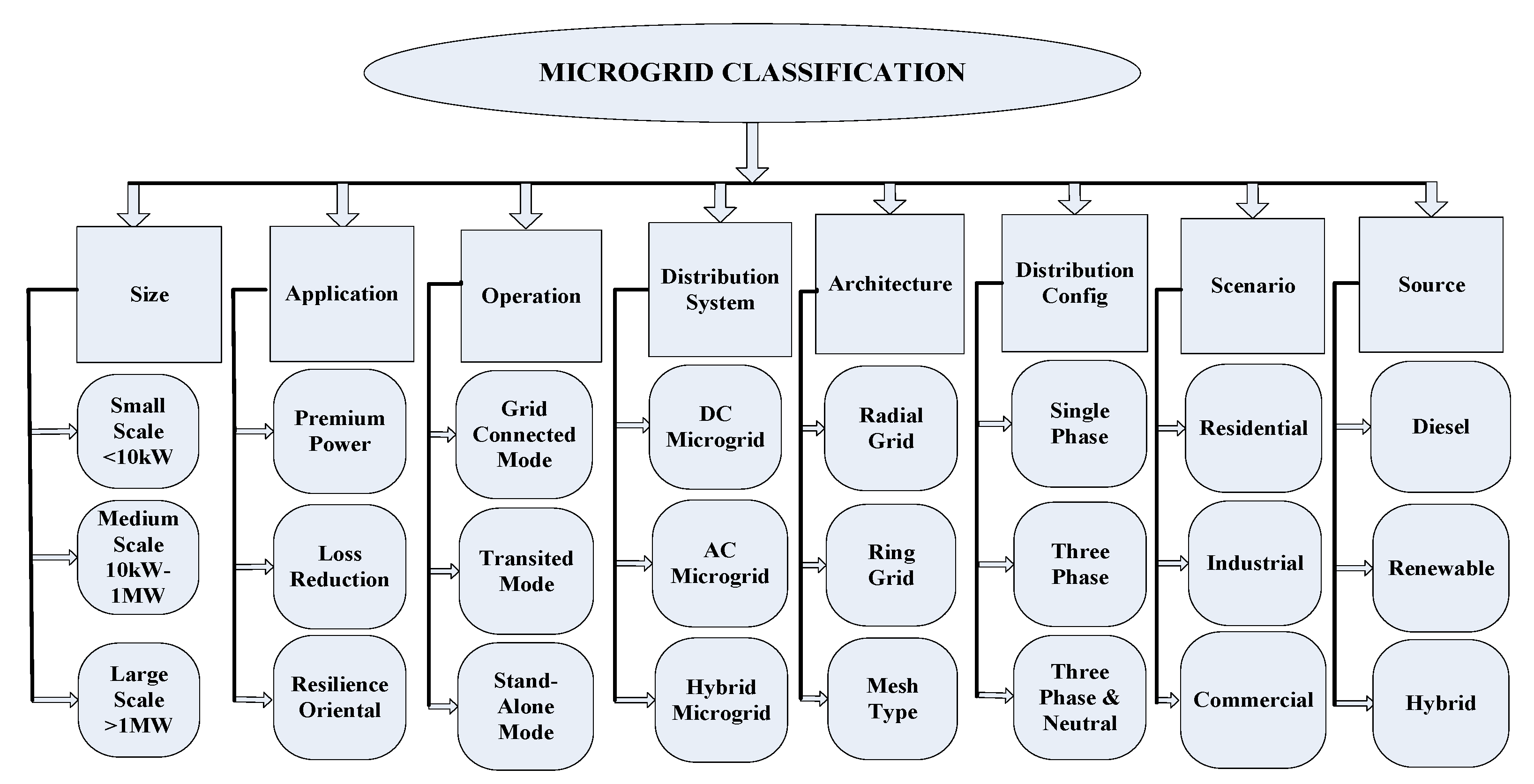
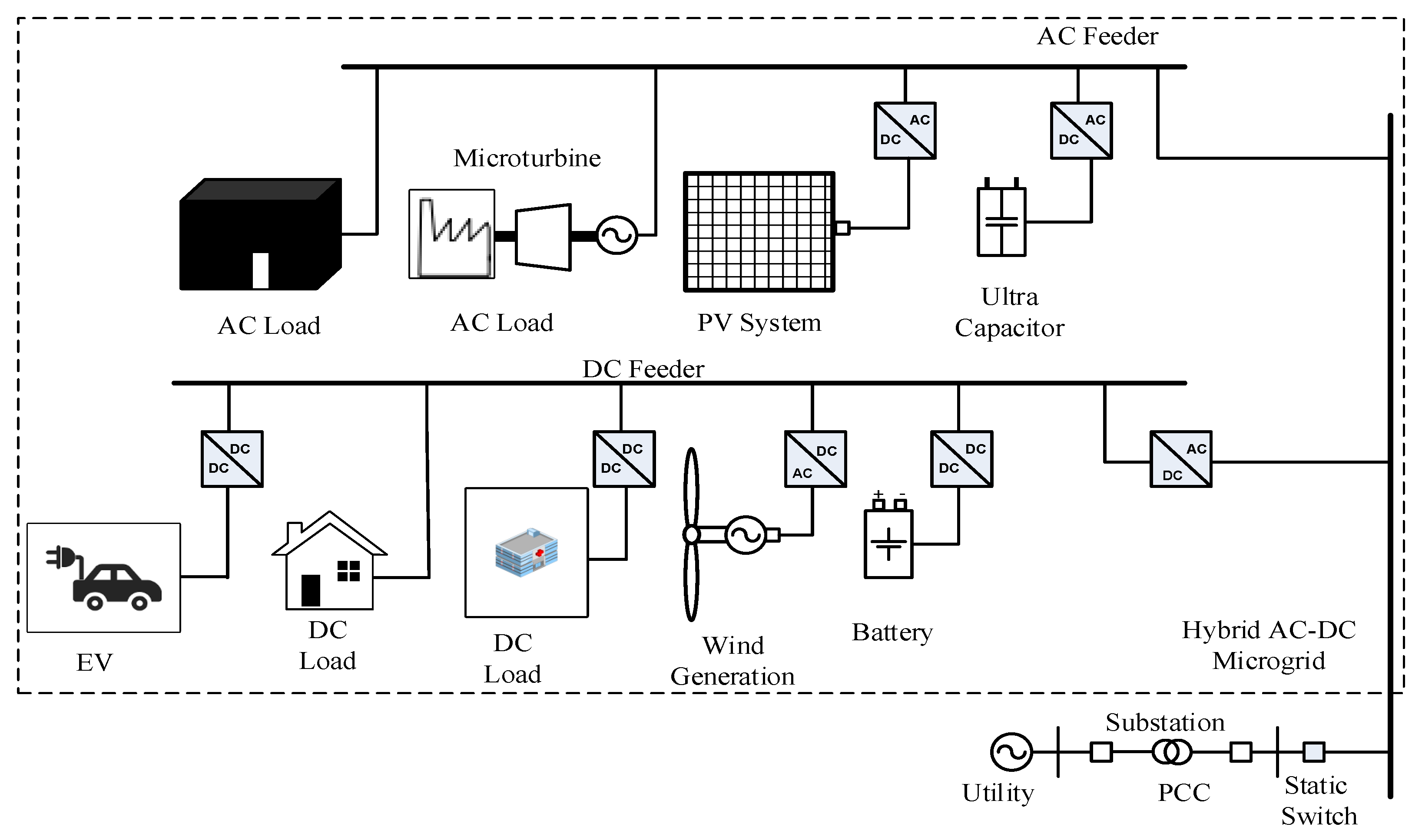
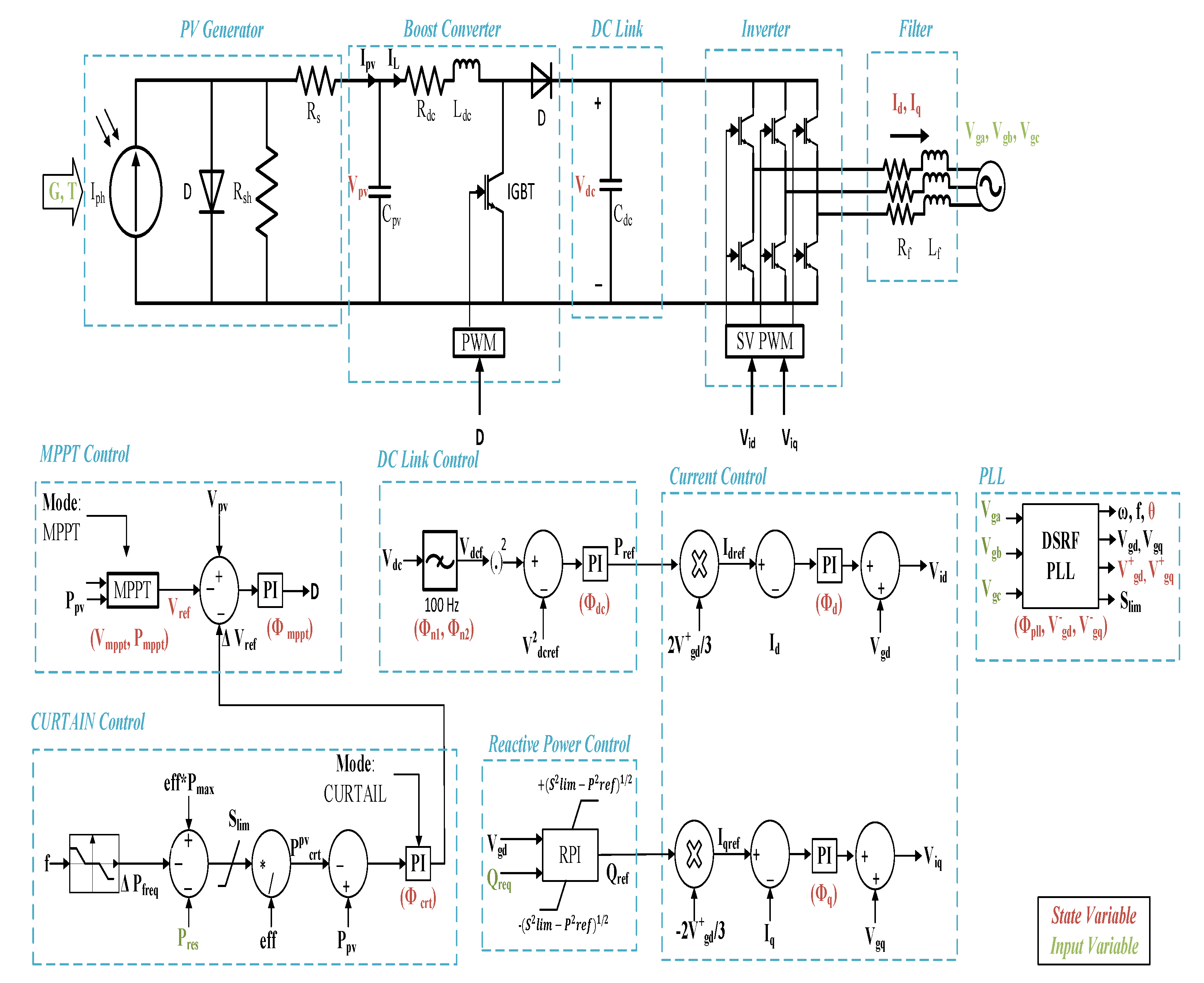

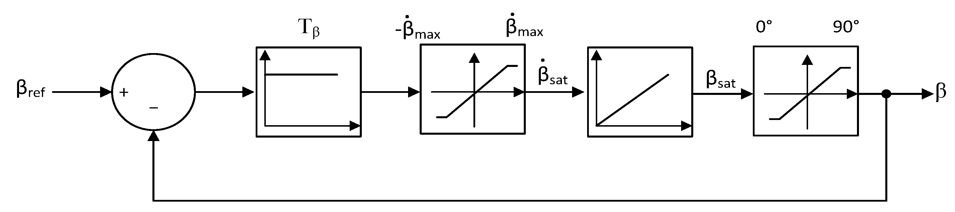
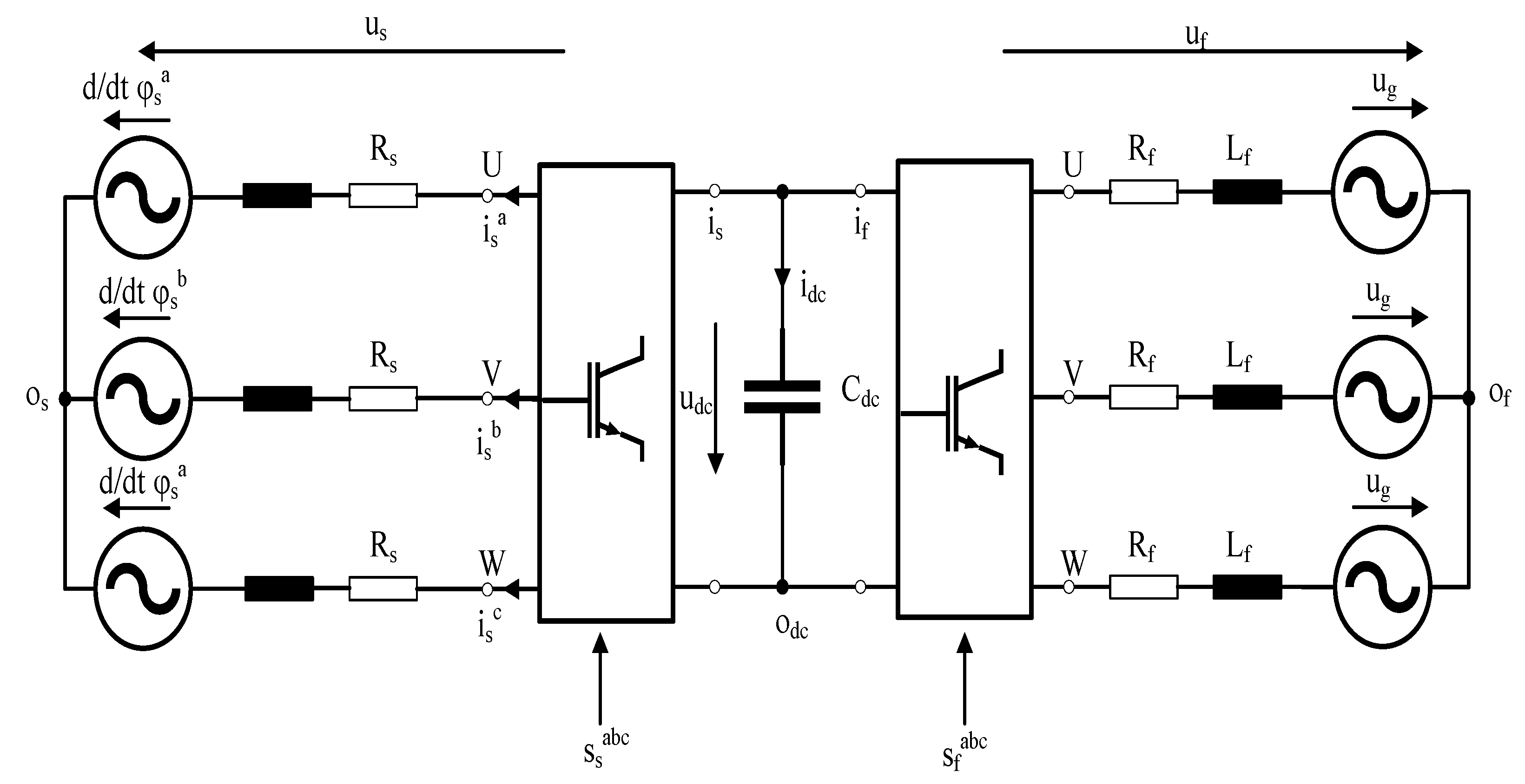
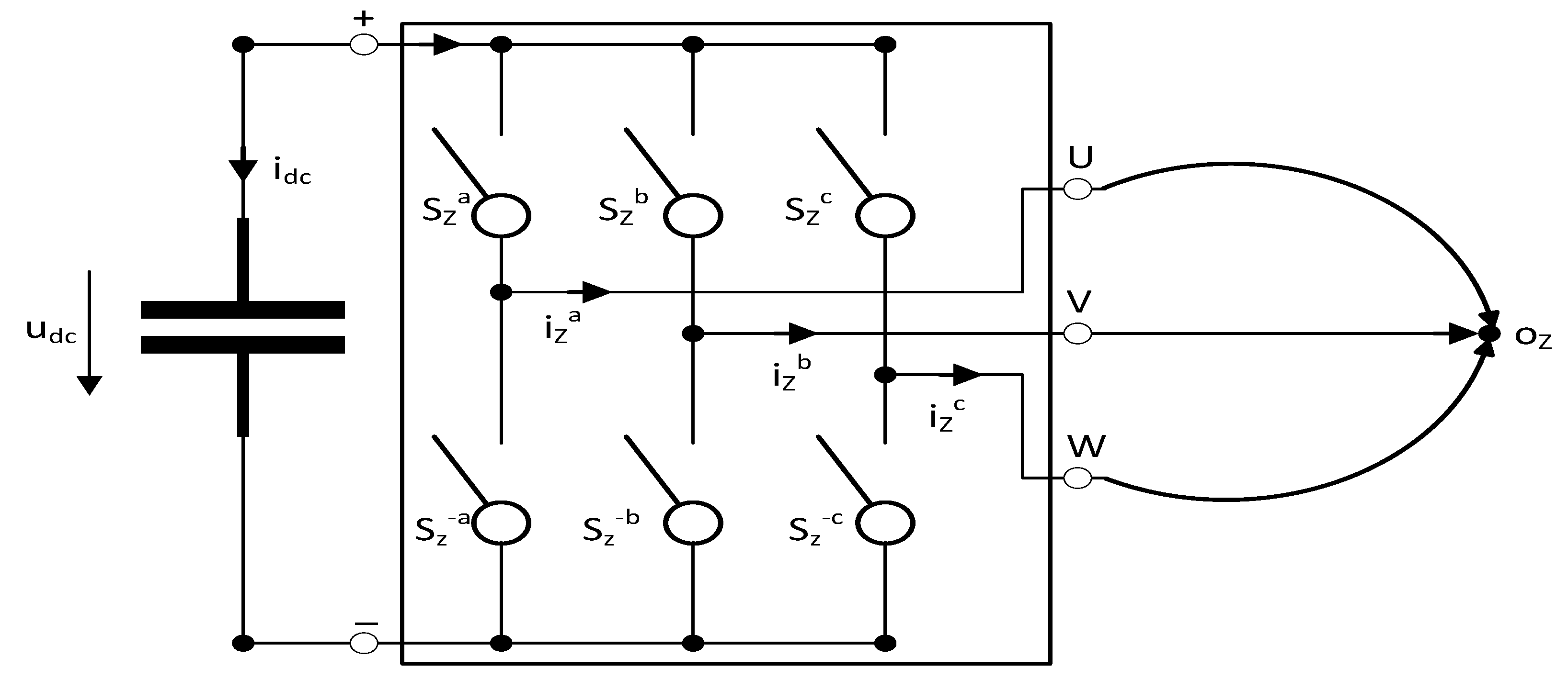

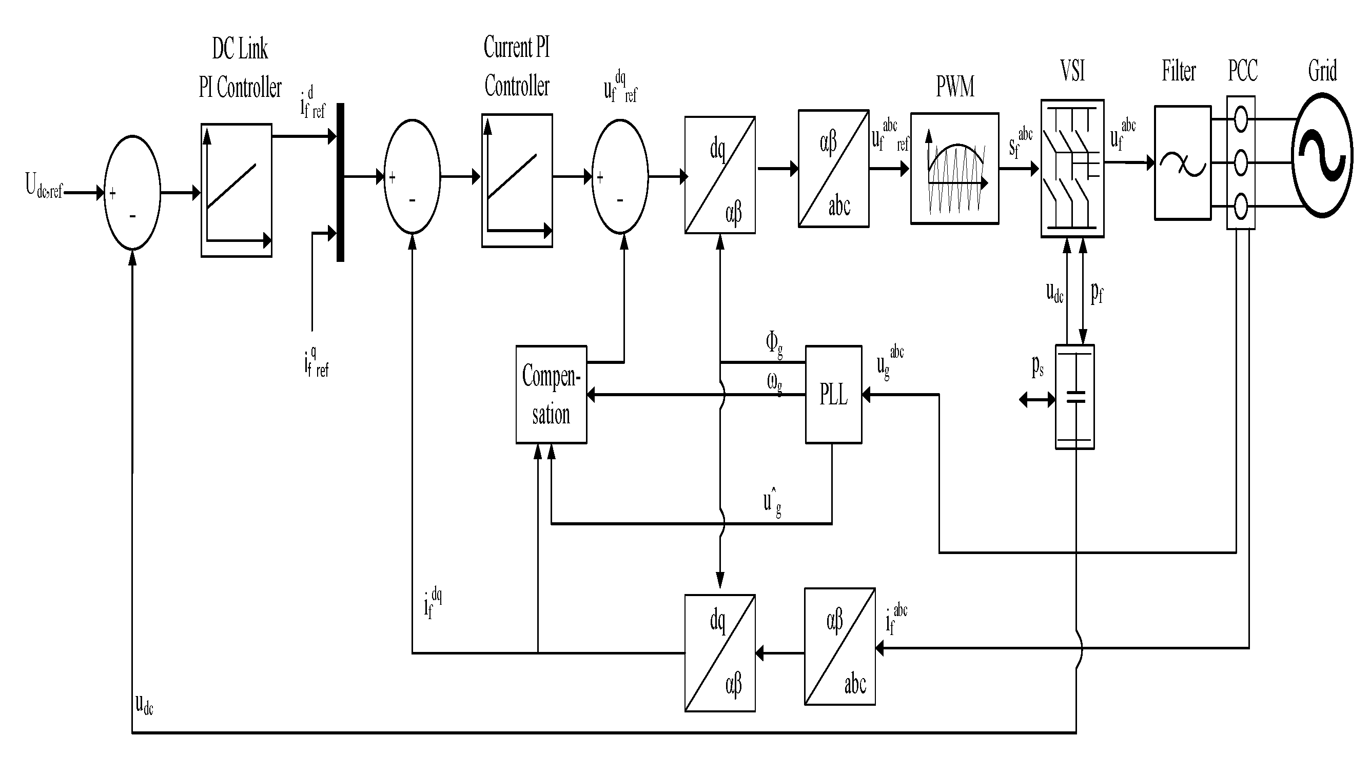
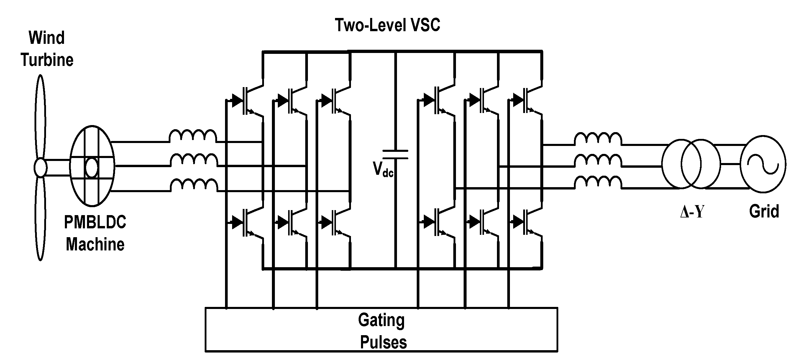


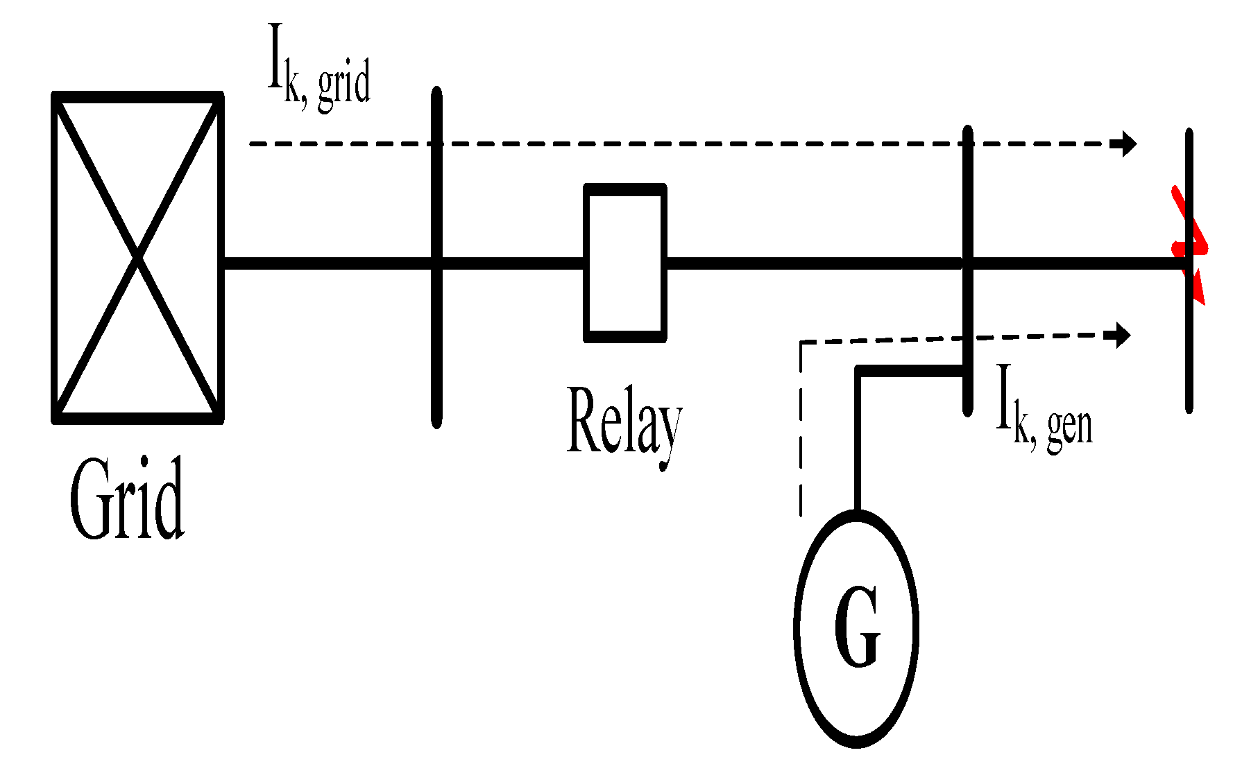
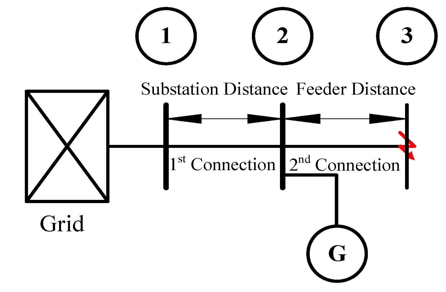
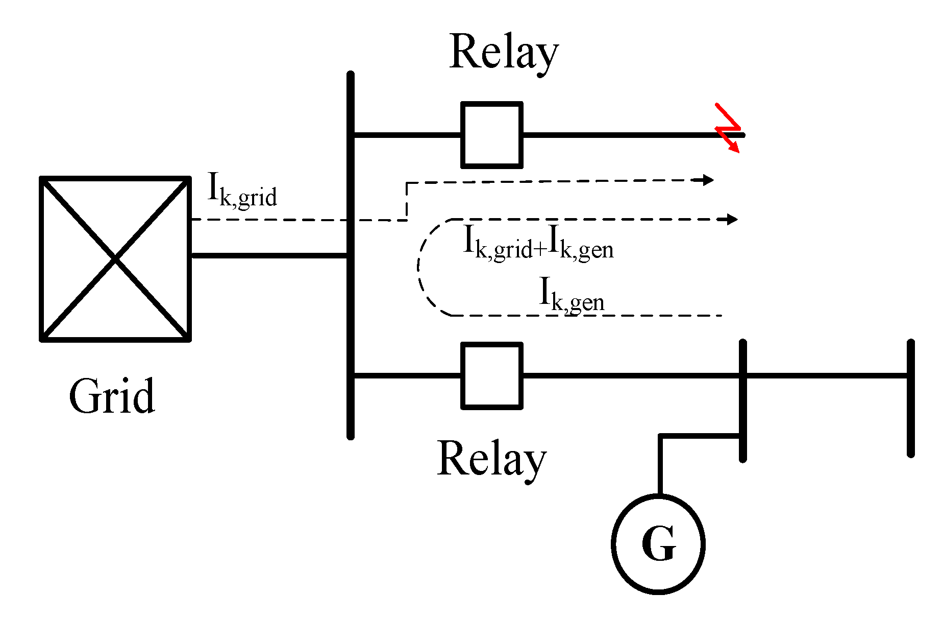


