Article

Speed Optimization for Container Ship Fleet Deployment Considering Fuel Consumption

1
Logistics Research Center, Shanghai Maritime University, Shanghai 201306, China
2
School of Management, Shanghai University of Engineering Science, Shanghai 201620, China
*
Author to whom correspondence should be addressed.
Sustainability 2021, 13(9), 5242; https://doi.org/10.3390/su13095242
Submission received: 27 March 2021 / Revised: 28 April 2021 / Accepted: 29 April 2021 / Published: 7 May 2021
(This article belongs to the Special Issue Sustainable Transport Planning and Decision-making)

Abstract

:
In recent years, low energy consumption has become the common choice of economic development in the world. In order to control energy consumption, shipping line speed optimization has become strategically important. to reduce fuel consumption, this study optimizes the container ship fleet deployment problem by adopting the strategy of adjusting each leg of each route’s sailing speed. To calculate fuel consumption more accurately, both sailing speed and the ship’s payload are considered. A multi-objective mixed integer nonlinear programming model is established to optimize the allocation of liner routes with multiple ship types on multiple routes. A linear outer-approximation algorithm and an improved piecewise linear approximation algorithm are used for linearization. If segments of an interval increase, the results will be more accurate but will take more time to compute. As fuel prices increase, to make trade-offs among economic and environmental considerations, the shipping company is adopting the “adding ship and slow down its speed” strategy, which verifies the validity and applicability of the established model.

1. Introduction

Although maritime transport is considered to be an environment-friendly mode of transport, due to over 80% of the world’s trade being carried by maritime transport [1], maritime transport has become a significant contributor to global greenhouse gas (GHG) emissions [2]. As GHG emissions of a ship are strongly related to its sailing speed [3], they can be reduced by optimizing sailing speed [4]. Hence, speed optimization has been proven to be one of the most effective operational measures to reduce GHG emissions.
In the context of GHG emissions reduction, shipping companies need to consider GHG emissions reduction when they make decisions on container ship fleet deployment (CSFD). For example, Maersk attaches great importance to reducing emissions [5]. GHG emissions from ships are directly proportional to fuel consumption [6]. The fuel consumption rate is a nonlinear function of sailing speed [7]. Thus, sailing speed optimization is one of the possible solutions to reduce ship fuel consumption. At the same time, the deployed number of ships on the route is dependent on sailing speed. The faster the speed, the fewer ships are configured in the route, and the slower the speed is, the more ships the route needs to be equipped. Therefore, shipping companies adopt the strategy of speed optimization to achieve GHG emission reduction and reduce ship operating costs, which is an effective means for the survival and profitability of ship owners and operators.
Liner shipping companies operate several container transportation routes and provide container transportation services for designated ports regularly. Container ships return to and from designated ports. When taking minimum cost as the objective function, the shipping companies are determined to reduce speed for each leg in the route so that the fuel consumption of their ships is minimized. However, this speed reduction causes the sailing time between ports to increase and requires more ships to be deployed on the route, which increases ship operating costs. Accordingly, the best way to balance operating costs and fuel consumption costs depends on sailing speed.
To bring flexibility to fleet deployment decisions, this paper considers sailing speed as a decision variable to make trade-offs among economic and environmental considerations. Regarding literature studies on fuel consumption, most studies only considered the effect of ship sailing speed, and few studies considered influence by payload (weight of containers on the ship) of a ship. In our work, to minimize the total costs, a mixed-integer nonlinear program (MINP) with container transshipment is proposed, which takes fuel consumption as the objective function and considers the influence of ship payload and ship speed. Meanwhile, for each route, we optimize each leg sailing speed, and we allocate appropriate ship types and deploy suitable number.
The remainder of this paper is organized as follows. Section 2 makes reviews the previous works. Section 3 develops a variation of an existing container ship deployment model, and the objective of reducing emissions. Section 4 proposes a series of techniques to a convert nonlinear model. Section 5 reports on computational experiments. Section 6 is the conclusion of the paper.

2. Literature Review

Container fleet deployment problem has become pressing for shipping lines. Christiansen et al. [8] claimed that shipping lines need to deploy suitable numbers and types of ships in order to maximize profits. Therefore, there are more and more researches focusing on container fleet deployment problems. Jaramillo and Perakis [9] addressed the fleet deployment problem by developing an integer linear programming model, but they did not consider container transshipment operations. As port-to-port cargo transportation may have many routes, it is necessary to consider container transshipment for the container fleet deployment problem. Gelareh and Pisinger [10] considered container transshipment but did not consider routing optimization because there is only one leg for each port pair. Wang and Meng [11] established a mixed-integer programming model, which incorporated container transshipment and routing optimization to realize container transshipment at any port and any number of times. Considering container transshipment operations will increase computational complexity, this is very realistic model.
In most of the existing container fleet deployment [12,13] models, it is assumed that the sailing speed is independent of the optimal fleet deployment decisions and set as constant, but in reality, the sailing speed is variable. Gelareh and Meng [14] studied the CSFD problem and proposed a MIP model with speed as a decision variable. Andersson et al. [15] studied CSFD problem with optimizing sailing speed simultaneously and established an integrated optimization model for RoRo shipping lines. Wang et al. [16] considered market uncertainty optimally regarding the CSFD problem with sailing speed optimization and developed a two-stage stochastic programming model. Zhen et al. [17] showed that to make ensure regular service frequency, shipping lines need to deploy more containerships when reducing sailing speed. In other words, the speed of the ship determines the number of ships deployed. Norstad et al. [18] stated that sailing speed is an important planning decision regarding the CSFD problem. Hence, it is essential to consider speed optimization for fleet deployment of a shipping network.
The speed of ships impacts fuel consumption costs, which in turn affects GHG emissions. Zacharioudakis et al. [19] proposed a practical solution to solve CSFD problem, which considered the effect of speed on fuel consumption. Du et al. [20] aimed to minimize fuel consumption by optimizing ship sailing speed and trim. Most studies assume that ship fuel consumption only depends on speed. Ronen [21] researched the daily fuel consumption function approach to the cubic of sailing speed. Wang and Meng [22] found the relationship between speed and fuel consumption by linear regression and calculated the fuel consumption function, which is entirely related to shipping speed (the index is between 2.7 and 3.3). Hence, it is essential to consider speed optimization for reducing fuel consumption.
However, in practice, various other factors affect a ship’s fuel consumption, such as ship hull conditions and payload. Ignoring the payload may lead to significant fuel consumption estimation errors. Research by Gkonis and Psaraftis [23] showed that at the same speed, ship fuel consumption was different between laden and ballast. The difference is approximately 25–30%. N.Psaraftis and A.Kontovas [24] provided a literature review of sailing speed optimization issues and showed that when speed was given, the fuel consumption of a ship varies with its payload. For example, the fuel consumption is different when the ship is full, in an intermediate loading condition, or empty. Therefore, it is necessary to comprehensively consider the influence of sailing speed and ship payload for reducing fuel consumption.
To accurately estimate fuel consumption, Xia et al. [25] used a nonlinear function to represent the relationship between ship payload and ship fuel consumption. However, there is a significant approximation error in the nonlinear approximation method, which may have seriously affected the quality of their solution. Wang et al. [26] studied shipping revenue management by adopting the fuel consumption rate function depending on sailing speed and ship payload, which developed a nonlinear fuel consumption rate function. However, they did not consider selecting the appropriate ship type according to the container flow. Zhen et al. [17] developed a multi-objective optimization model to solved CSFD problem considering the influence of container transshipment and fuel consumption. However, they assumed that fuel consumption cost only depended on sailing speed, and each port operation time was given.
To overcome the aforementioned limitations, our work is based on Wang and Meng’s [11] proposed model, which assumed that each leg of a ship’s sailing speed of route is deterministic. To relax this assumption and optimize each leg sailing speed of route, we put sailing speed optimization incorporate into CSFD problem models as a decision variable. As the number of deployed ships and fuel consumption depends on sailing speed, in order to balance economic and environmental considerations, we proposed a multi-objective mixed integer programming model to optimize sailing speed, which minimizes the total costs and total fuel consumption cost. The proposed model was nonlinear, and we use liner techniques to linearize it.
In this article, we primarily contribute to the relevant literature in the following ways. First, we investigate the theoretical and practical implications of fleet deployment that considers container transshipment and optimizes ships’ speeds. We propose a mixed-integer nonlinear program and linearize the nonlinear expressions in the developed models. Second, a linear outer-approximation algorithm and an improved piecewise linear approximation algorithm are applied to further approximate nonlinear functions. Thus, we develop a mixed-integer linear program whose problems can be solved by on-the-shelf solvers.

3. Mathematical Model Formulation

Shipping lines regularly serve a set of ports. The ports’ order was given and formed a closed loop, which provided customers with circular liner transportation services and ensured weekly flights. The shipping lines allocated the appropriate number and types of ships on the route. Figure 1 shows the shipping network of composition by three routes. Containers attached to ports on different routes require transshipment at public ports to meet the transportation demand of OD flows. For example, container transshipment operations of route 1 and route 3 in Figure 1 can be performed at ports 1 and 3. However, the transshipment operation at the transit port will increase the handling capacity of containers, thus increasing the transshipment cost.

3.1. Parameter and Variable Definition

The parameter and variable definitions in this study are introduced in Table 1.

3.2. Fuel Consumption Cost

N. Psaraftis and A. Kontovas [24] proposed the fuel consumption non-linear function, which depends on the ship sailing speed and ship payload, in which the daily bunker consumption rate is expressed as f s , w , s is the sailing speed, and w   is the ship payload of each segment. A realistic approximation of fuel consumption function is   f s , w = c 1 r q + s c 2 r w + A c 3 r with c 1 r , c 2 r , c 3 r   and q   constants such as c 1 r > 0 , c 2 r 3 , c 3 r 0 and q 0 , and A is the weight of the empty container ship. As the sailing speed and payload of different segments of each route are different, we assume that q = 0 and A = 0 ; the daily fuel consumption function of leg i on route r is equal to   f s r i , w r i = c 1 r s r i c 2 r w r i c 3 r . As far as we know, the leg i length of route r is L r i , Then, the leg i sailing time of route r can be calculated by L r i / s r i . β is the fuel price, 24 is the hour of the day, and the ship fuel consumption cost expressed as:
f F C = β · r R i I r c 1 r s r i c 2 r 1 w r i c a r · L r i / 24
The developed model in this study optimizes the sailing speed of each leg. As the number of deployed ships and fuel consumption depend on sailing speed, it is beneficial for container shipping lines to optimize the sailing speed of each leg when they decide to minimize the total fuel consumption cost and total operating costs. This study adopts a realistic function of ship fuel consumption rate; optimizing the sailing speed of each leg allows the fuel consumption cost of ships in sailing to be more precisely estimated, which improves the management accuracy for liner shipping companies.

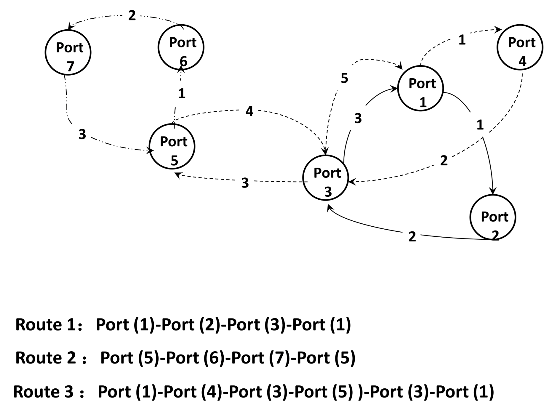
3.3. Container Ships’ Fleet Deployment Model

The objective function of the model is to minimize the cost of ship fuel consumption and the total operating cost of the fleet in the weekly plan, which is defined as a Constraint (2)–(8). Where f C F is expressed as a fixed cost of ship navigation,   f C B is expressed as occupancy cost of berthing berth in port, f C T is expressed as total container transshipment cost, f C O is expressed as container handling cost, f C I is expressed as the cost of renting ships, and f R O is expressed as proceeds from charter-owned ships.
Minimize   f = f F C + f C F + f C B + f C T + f C O + f C I f R O
f C F = r R , v V r m r , v · C v o p r + C r , v f i x · x r , v
f C B = r , i I r , v V r C P r , i , v b e r · T P r , i , v c o n t · z r , v , i
f C T = p P C p t r a n · z p t r a n
f C O = o , d P C o l o a d + C d d i s c · D o , d
f C I = v V C v i n · n v i n
f R O = v V C v o u t · n v o u t
s.t.
v V r x r , v = 1 , r
m r , v M 1 · x r , v , r , v
168 · m r , v + M 2 · 1 x r , v i I r L r i / s r i + i I r T P r , i , v c o n t · z r , v , i , r , v V r
z v , r , i M 3 · x r , v , r , i I r , v V r
z v , r , i + M 4 · 1 x r , v o z o , r , i l o a d + z o , r , i d i s c , r , i I r , v V r
o z o , r , i f l o w v V r Q v · x r , v 0 , r , i I r
z o , r , i 1 f l o w + z o , r , i l o a d z o , r , i d i s c = z o , r , i f l o w , r , i I r , o
r R i , i I r , i z o , r , i d i s c z o , r , i l o a d = D o , d , o d  
z o , r , i f l o w = 0 , r , i I r , o = P r , i + 1
z o , r , i d i s c = 0 ,   , r , i I r , o = P r , i
r R p , i R p m r , v n v i n + n v o u t = N v o w n , v
n v i n N v i n , v
z p t r a n = r R r , i I r , p , o P z o , r , i l o a d + z o , r , i d i s c d D p , d o D o , p , p
w r , i i n w r , i w r , i m a x , r , i I r
o z o , r , i f l o w + e r , i = w r , i , r , i I r
s r , i m i n s r , i s r , i m a x , r , i I r
Constraint (9) ensures that each route deployed only one type of ship; Constraints (10) and (11) indicate that the number of ships configured for each route can meet the service demand in the weekly plan, 168 represents the number of hours in a week, set M 1 and M 2 to 9999 ; Constraints (12) and (13) define the relationship between variables, M 3 and M 4   set to 9999 ; in Constraint (14) the container transportation volume of each leg cannot exceed the ship’s carrying capacity; and Constraint (15) represents the flow of conservation. The carrying capacity before berthing at port i , plus the amount of containers loading and subtract the amount of unloading, is equal to the shipping capacity leaving the port; Constraint (16) ensures that all container transportation needs between ports are served; Constraint (17) indicates containers from the port o will not be shipped back to the port o ; Constraint (18) indicates containers from the port o will not be unloaded at the port o ; Constraint (19) indicates conservation of the number of ships; Constraint (20) indicates that the number of chartered ships cannot exceed the upper limit; Constraint (21) indicates the weight of ballast water required to ensure the stability of the ship’s navigation; Constraint (22) is that for safety or other purposes, the ship’s payload should be within the range; Constraint (23) the weight of ballast water needed to ensure the stability of ship navigation; and Constraint (24) is the range of ship speed.

4. Linearization of the Model

The above model for fleet deployment with sailing speed and routing optimization has a nonlinear objective (1) with nonlinear terms s r i c 2 r 1 w r i c 3 r and nonlinear Constraint (11) with nonlinear term L r i / s r i . Due to the following reasons, we linearize these formula expressions. First, although some mixed-integer program solvers (e.g., Gurobi) can handle nonlinear objective functions, it is challenging to solve models with complicated nonlinear objectives, especially nonlinear constraints. Second, customized linearization techniques are applicable, as studied by many pioneering studies in the literature. Third, after preliminary study and tests, the devised model in this study is not solvable directly when the nonlinear objective and constraints are considered. Therefore, we adopted the linearization technique to convert the model to a linear one. The logical structure is expressed as: first, the reciprocal of the speed to linearize nonlinear Constraint (11). Then, linearize the ship’s fuel consumption objective Function (1). Finally, perform bilinear optimization on the Constraint (30).

4.1. Linearization of the Reciprocal of Sailing Speeds

Due to 1 / s r i that is nonlinear, take its reciprocal as the decision variable   u r i . In general, the sailing speed is different on each leg of the route, and within the speed interval   s r i m i n , s r i m a x , this speed interval depends on mechanical power engine size and economic factors. Therefore, u r i lower bound is u r i m i n = 1 / s r i m a x and upper bound is u r i m a x = 1 / s r i m i n . Then, the Constraint (11) becomes a linear constraint and can be rewritten by Constraint (27)
u r i = 1 / s r i
u r i m i n u r i u r i m a x , r , i I r
168 · m r , v + M 2 · 1 x r , v i I r L r i · u r i + i I r T P r , i , v c o n t · z r , v , i , r , v V r

4.2. Linearization of the Objective Function of Fuel Consumption Cost

The objective function of fuel consumption cost can be expressed as follows:
β · r R i I r c 1 r u r i 1 c 2 r · w r i c 3 r · L r i / 24
The fuel consumption cost objective Function (28) can be further linearization by introducing the auxiliary variables: B r i , r i ,   and Λ r i , transformed to the following objective Function (29) and Constraints (30)–(32).
β · r R , i I r B r i
24 · B r i / c 1 r · L r i r i · Λ r i
r i u r i 1 c 2 r , r , i I r
Λ r i w r i c 3 r , r , i I r

4.3. Underestimating Bilinear Terms

Al-Khayyal and Falk [27] showed that the bilinear term x · y tightest convex lower bound is obtained via the following relationship m a x x L y + y L x x L y L ,   x U y + y U x x U y U in the interval x L ,   x U × y L , y U . Due to the fact that r i and Λ r i have the lower limit and upper limit, Wang et al. [26] showed that r i · Λ r i term is bilinear. The lower bound for r i · Λ r i in the interval u r i m a x 1 c 2 r , u r i m i n 1 c 2 r and w r i m i n c 3 r , w r i m a x c 3 r is obtained by following Constraint (33)
r i · Λ r i = m a x u r i m a x 1 c 2 r · Λ r i + w r i m i n c 3 r · r i u r i m a x 1 c 2 r · w r i m i n c 3 r u r i m i n 1 c 2 r · Λ r i + w r i m a x c 3 r · r i u r i m i n 1 c 2 r · w r i m a x c 3 r
Therefore, Constraint (30) can be relaxed by adding linear Constraint (34) and Constraint (35):
24 · B r i / c 1 r · L r i u r i m a x 1 c 2 r · Λ r i + w r i m i n c 3 r · r i u r i m a x 1 c 2 r · w r i m i n c 3 r
24 · B r i / c 1 r · L r i u r i m i n 1 c 2 r · Λ r i + w r i m a x c 3 r · r i u r i m i n 1 c 2 r · w r i m a x c 3 r

5. Approximation Algorithm

The logical structure of the approximation algorithm is expressed as: first, a linear outer-approximation algorithm developed to handle nonlinear Constraint (31). Then, an improved piecewise linear approximation algorithm was applied to linearization nonlinear Constraint (32). Last, it is converted into a linear mixed-integer programming model.

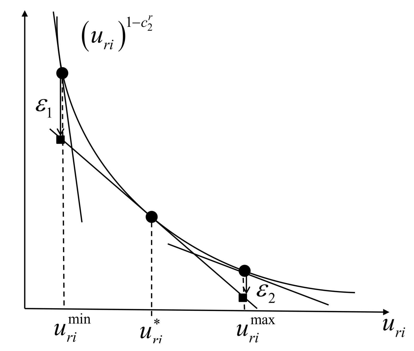
5.1. Linear Outer-Approximation Algorithm

The principle of the algorithm is to divide the nonlinear characteristic curve into several linear segments and approximate it by a series of tangent lines. Therefore, the interval u r i m i n , u r i m a x   is subdivided into several segments. For each segment, the function u r i 1 c 2 r is approximated by a tangent line.
Proposition 1.
u r i 1 c 2 r is convex in u r i
Proof. 
The first-order derivatives of u r i 1 c 2 r are denoted by u r i 1 c 2 r and can be calculated as:
u r i 1 c 2 r =   1 c 2 r   ·   u r i c 2 r
The second-order derivative of u r i 1 c 2 r   with respect to u r i is denoted by u r i 1 c 2 r and can be calculated as:
u r i 1 c 2 r = 1 c 2 r   ·   c 2 r   ·   u r i c 2 r 1
According to Wang and Meng [22], the coefficient c 2 r is greater than 2, hence the second-order derivative u r i 1 c 2 r > 0 . When on the interval u r i m i n , u r i m a x , u r i 1 c 2 r   is convex. □
In order to approximate u r i 1 c 2 r , Figure 2 shows the tangent lines. To control the approximation error ε 1 , some tangent lines are generated a priori. Then, whether the calculation gap is larger than ε 1 is determined. If so, the interval is further subdivided to obtain more approximate tangent lines. Otherwise, the approximation gap is acceptable, and the tangent point is recorded in the set Ω r i .
At tangent point u r i k , the tangent line of the function u r i 1 c 2 r can be derived as:
u r i k 1 c 2 r + u r i k 1 c 2 r × u r i u r i k , r R ,   i I r , u r i k
where Ω ε 1 is the tangent points set of function u r i 1 c 2 r , when given ε 1 , the procedure to obtain set Ω ε 1 is shown in Algorithm 1. Then, the nonlinear Constraint (31) can be expressed as:
r i   1 c 2 r u r i k c 2 r u r i + c 2 r u r i k 1 c 2 r , r R ,   i I r , u r i k Ω r i ε 1
Algorithm 1. The procedure of linear outer-approximation algorithm to obtain tangent point sets.
Input:Convex function u r i 1 c 2 r , the tangent point set Ω r i . The lower limit and upper limit of u r i is     u r i m i n , u r i m a x , the approximation relative error ε 1
Output:the tangent point set Ω r i ε 1  
Step 1 Calculate   the   midpoint   u r i m i d of the interval   u r i m i n , u r i m a x ; u r i m i d can be carried out by the bisection search method
Step 2At tangent point u r i m i d , the tangent line is defined as u r i m i d 1 c 2 r + u r i m i d 1 c 2 r × u r i u r i m i d
Step 3Calculate the relative approximation error of points u r i m i n and u r i m a x according to
ε l = u r i m i n 1 c 2 r u r i m i d 1 c 2 r u r i m i d 1 c 2 r × u r i m i n u r i m i d
ε r = u r i m a x 1 c 2 r u r i m i d 1 c 2 r u r i m i d 1 c 2 r × u r i m a x u r i m i d
Step 4If ε l > ε or ε r > ε , then branch the feasible range of u r i is divided into two ranges:   u r i m i n , u r i m i d and   u r i m i d , u r i m a x , and the tangent point set Ω r i ε 1 = Ω r i ε 1   u r i m i d
In one branch u r i   u r i m i n , u r i m i d , repeat the above step 1 to e step 4 until the stop criterion is reached
In the other branch u r i   u r i m i d , u r i m a x , repeat the above step 1 to e step 4 until the stop criterion is reached
Stop criterion check: if ε l < ε and ε r < ε , stop and output the current solution. Otherwise, go to Step4.
Step 5Return output Ω r i ε 1  

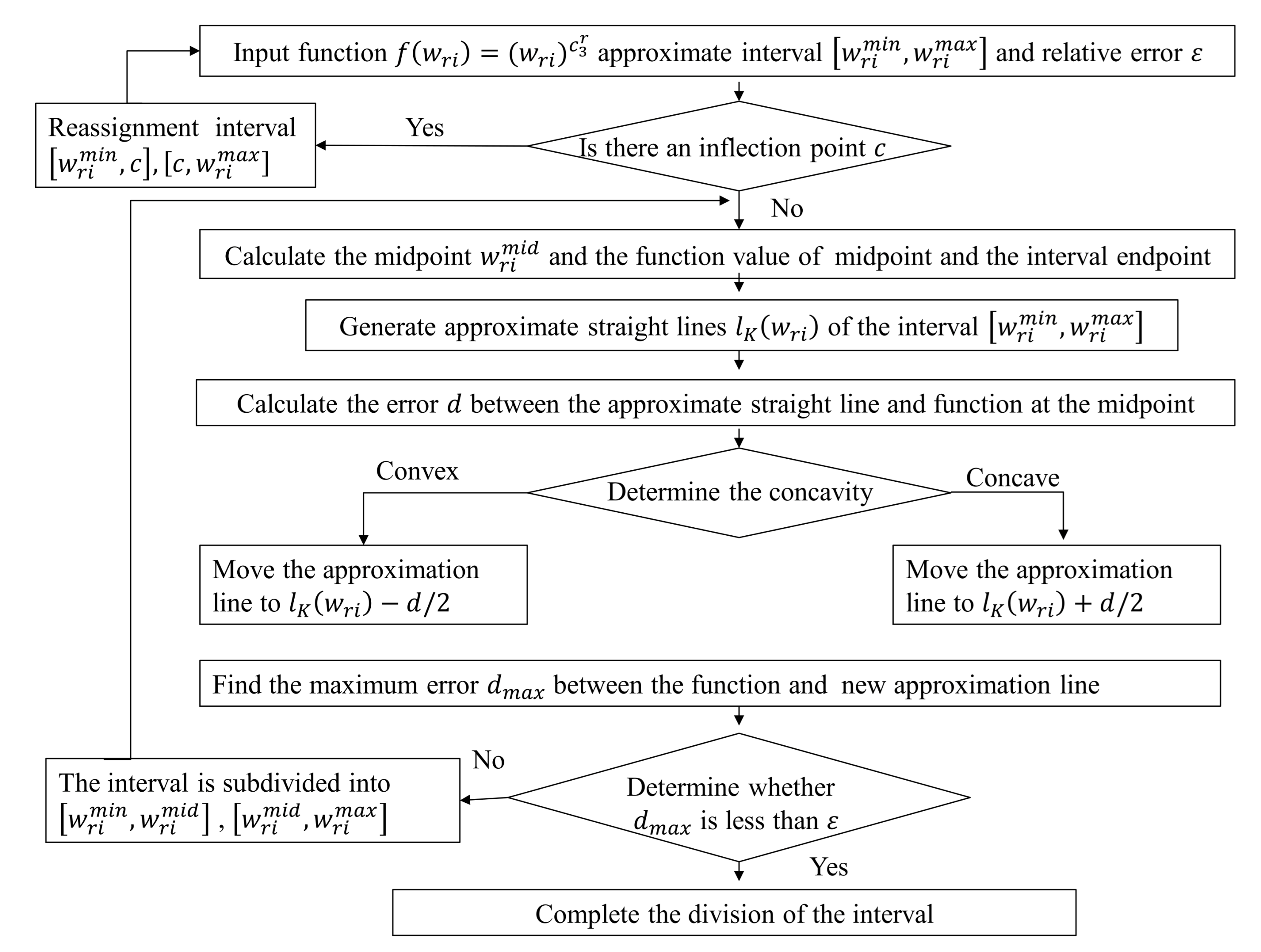
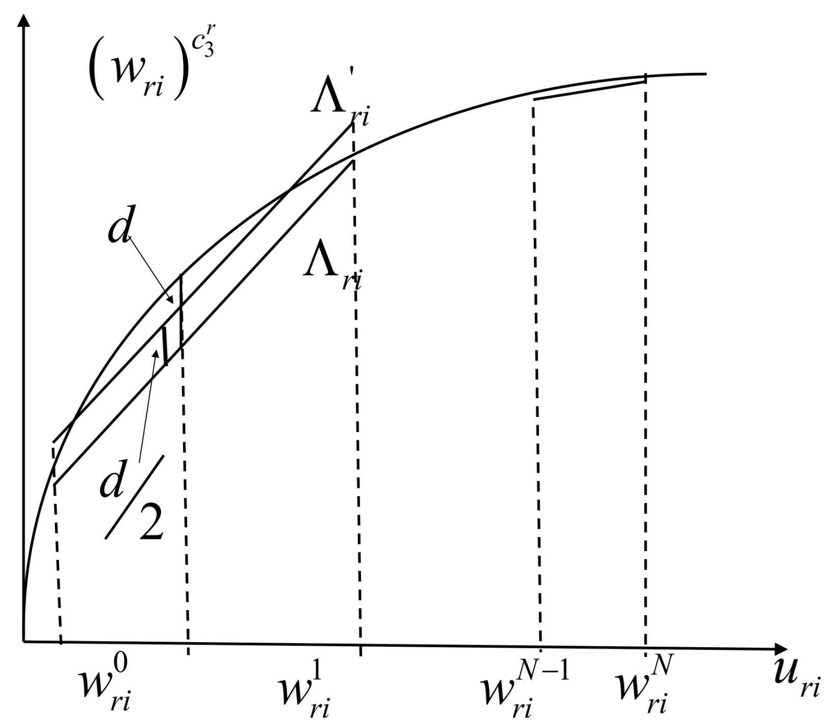
5.2. Improved Piecewise Linear Approximation Algorithm

The principle of the algorithm is to divide the nonlinear characteristic curve into several linear segments and approximate the characteristic curve in each segment with a straight-line section. Therefore, the interval w r i m i n , w r i m a x is subdivided into several segments; for each segment, the function w r i c 3 r is approximated by the linear function l K w r i .
Proposition 2.
  f w r i = w r i c 3 r is a continuous functionon the interval w r i m i n , w r i m a x , then the piecewise linear function l K w r i is uniformly approximated to f w r i .
Proof. 
Since f w r i is continuous on w r i m i n , w r i m a x , then f w r i is uniformly continuous on w r i m i n , w r i m a x . That is, for any given ε > 0 , there exists δ ε > 0 ; for any w r i , w r i w r i m i n , w r i m a x , as long as w r i w r i < δ ε , there is f w r i f w r i < ε .
The interval w r i m i n , w r i m a x is divided into K segments; a j , j = 1 , , K , K + 1 is expressed as the breakpoints of the piecewise linear function. Command w r i m i n = a 1 < a 2 < a 3 < < a K < a K + 1 = w r i m a x . When K > 1 / δ ε , for w r i 1 , w r i 2 a j , a j + 1 , there is f w r i 1 f w r i 2 < ε .
m i n f a j , f a j + 1 l K , j + 1 w r i m a x f a j , f a j + 1 , l K , j + 1 w r i indicates the function section for the interval a j , a j + 1 , that is, the j + 1 segment linear function. So m i n f j + 1 w r i f a j , f j + 1 w r i f a j + 1 f j + 1 w r i l K , j + 1 w r i m a x f j + 1 w r i f a j , f j + 1 w r i f a j + 1 , f j + 1 w r i represents the corresponding function of f w r i on interval a j , a j + 1 , which is f j + 1 w r i l K , j + 1 w r i < m a x f j + 1 w r i f a j , f j + 1 w r i f a j + 1 < ε , then for w r i j = 0 n 1 a j , a j + 1 , there is f w r i l K w r i < ε . Therefore, on interval w r i m i n , w r i m a x , there is a piecewise linear function l K w r i that is uniformly approximated to the continuous function f w r i . □
Therefore, this paper proposes an improved function piecewise linear approximation algorithm, which can complete the optimal selection of the number of pieces under the premise of known accuracy, so that the calculation function error is within a specific range. The main idea of the algorithm is: further subdivide the function interval with more significant errors, avoid the waste of segmentation of the smooth part of the curve, and reduce the computational complexity. The algorithm flow implemented in this paper is shown in Figure 3. The calculation of the segment interval is completed by an iterative method.
On each segment interval, the concavity of the approximated function and whether the function has an inflection point in the interval are judged. For interval w r i m i n , w r i m a x , the approximation lines can be generated as follows:
Function Generate approximate straight lines l K w r i two endpoints of the curve f w r i = w r i c 3 r in interval w r i m i n , w r i m a x are A = w r i m i n , w r i m i n c 3 r and B = w r i m a x , w r i m a x c 3 r , the equation of a straight line is found through these two points. Assuming the point C = w r i , l K w r i is on a straight line, hence the slope of the line AC and the line AB are the same, expressed as:
l K w r i w r i m i n c 3 r / w r i w r i m i n   =   w r i m a x c 3 r w r i m i n c 3 r / w r i m a x w r i m i n
By transforming the formula, we can get an approximately straight line:
l K w r i   =   w r i m a x c 3 r w r i m i n c 3 r w r i m a x w r i m i n · w r i + w r i m a x · w r i m i n c 3 r w r i m i n · w r i m a x c 3 r w r i m a x w r i m i n
The approximation error between straight line and function is expressed as   d =   f w r i     l K w r i . Then, the approximation error is calculated between the approximate straight line l K w r i and function w r i c 3 r at the midpoint w r i m i d . The concavity of the function w r i c 3 r is judged; the following lemma proves the function property is nonconvex:
Proposition 3.
w r i c 3 r is concavein w r i
Proof. 
The second-order derivative of w r i c 3 r   with respect to w r i denoted by w r i c 3 r can be calculated by constraint
w r i c 3 r = c 3 r c 3 r 1 w r i c 3 r 2
According to the N.Psaraftis and A.Kontovas [24], the coefficient c 3 r is between 0 and 1; hence, the second-order derivative w r i c 3 r < 0 . So, the function w r i c 3 r   is concave when w r i takes value in interval w r i m i n , w r i m a x . □
Therefore, the function w r i c 3 r is concave, then the approximation line is moved to l K w r i   +   d / 2 , shown in Figure 4. The maximum error is found between the function and the new approximation line on the interval   w r i m i n , w r i m a x , expressed as d m a x   =   f w r i l K w r i   +   d / 2 . Then, the derivative of the function d m a x is taken and the derivative is made equal to 0, to obtain the value of w r i * . At last, w r i * is substituted into the function d m a x . The maximum error between the approximation line and function is obtained and then compared with the given error ε 2 : if the maximum error d m a x > ε 2 , the interval of the approximation is further subdivided and the breakpoints of the piecewise linear function set W r i = W r i w r i m i d , then we branch the feasible range of w r i into two ranges:   w r i m i n , w r i m i d and   w r i m i d , w r i m a x . If the maximum error d m a x < ε 2 , the continuous subdivision of the segment is stopped.
w r i is divided into K segments in the interval w r i m i n , w r i m a x , which is determined by improved piecewise linear approximation algorithm, the breakpoints of the piecewise linear function set expressed as W r i K   =   w r , i , k , k M , where M =   1 , 2 , K , K + 1 ; by introducing the auxiliary variable η r i k and π r i k , then, the nonlinearity Constraints (32) can be rewritten as:
Λ r i k M η r , i , k · w r , i , k c 3 r , w r , i , k W r i K , r R ,   i I r
w r i = k M η r , i , k · w r , i , k , w r , i , k W r i K , r R ,   i I r
k M η r , i , k = 1 , r R ,   i I r
k M K + 1 π r , i , k = 1 , r R ,   i I r
η r , i , 1 π r , i , 1 , r R ,   i I r
η r , i , k π r , i , k 1 + π r , i , k , r R ,   i I r k = 2 , , K
π r , i , k = 0 , 1 , k M K + 1
η r , i , k 0 , k M

5.3. Mixed Integer Linear Programming Model

In summary, through the above series linearization operations, the nonlinear MINP model can become an equivalent mixed-integer linear programming MIIP.
Minimize f = β · r R , i I r B r i + f C F + f C B + f C T + f C O + f C I f R O
s.t.  Constraints (3)–(10), Constraints (12)–(24), Constraints (25)–(27), Constraints (34)–(35), and Constraints (37)–(46).

6. Numerical Experiments

6.1. Parameter Setting

The numerical experiment data are derived from reference Wang and Meng [11], which contains 46 ports and 12 routes. Table 2 shows the values of parameters for different ships. Table 3 shows parameters related to the 12 ship routes. Table 4 shows the ship fixed operating costs of 12 ship routes. The value range of container flow between ports is U 0 , 30 . The loading cost C p l o a d and discharge cost C p d i s c are 150; the container transshipment cost is 200. For the value of c 1 r ,   c 2 r , and c 3 r from literature Wang et al. [26], the coefficient c 1 r is 0.0006, c 2 r is 2.5, and c 3 r is 0.56. The model was implemented in Python version 3.8 and solved by using GUROBI version 8.1.1. We carry out calculation experiments run by an Intel 2.7 GHz core i3 CPU and 16GB RAM machine with Windows 10.
Wang et al. ’s [26] research shows a small approximation error means a large number of segments and more computation time, so they set minimum linear outer-approximation error at 1 × 10 3 . Yang and Xing [28] set the number of line fragments for linear outer-approximation to be 100. We set the number of line fragments for linear outer-approximation to be 68 and 135. For piecewise linear function approximation error, Wang et al. [26] set the number of line segments 8. To obtain higher accuracy, we set the number of line segments to 11 and 22, providing a more accurate optimal solution. We composed four scenarios according to the combination of the different approximation error ε 1 and piecewise linear function approximating error ε 2 , as shown in Table 5.

6.2. Sensitivity Analysis of Various Fleet Costs

According to the four scenarios composed of different error accuracy, the total fleet operation cost is calculated, along with the ship consumption cost, the total cost of berthing operation, and the total cost of container transshipment under four scenarios. Results of Scenario 2 compared to Scenario 1 and Scenario 4 compared to Scenario 3 are shown in Table 6:
The negative values of 1 and 2 show that the number of segments within the range of ship’s payload increased, as shown in Table 6. The same as 3 and 4 . If the ship’s fuel consumption estimation is accurate, then the total cost of the fleet and fuel consumption cost in the weekly plan is reduced, which shows the effectiveness of the model. More segments will incur more accurate results, but the calculating time will be longer. For example, the calculation time of scenario 2 is greater than scenario 1. The fluctuation range of container transshipment cost is small, which indicates that when the OD flow of container is determined, the container transshipment network is formed and the container transit port is determined, so the reduction of calculation accuracy has little effect on it.

6.3. Analyze the Relationship between Ship Deployment and Sailing Speed

As the unit fuel consumption cost of ships changes, so does the type and quantity of ships deployed on routes 2 and 6, as well as the optimal sailing speed for different legs of the two routes.
Table 7 shows that with the increase of unit fuel consumption cost of ships, the types and number of ships deployed have changed, which means shipping companies need to adjust the deployment of appropriate ship types and determine the appropriate number to reduce the total operation cost of fleet deployment. For the ships deployed in route 2, when the unit fuel consumption cost changes from 100 to 200, one medium-sized ship is replaced by two small-sized ships. It can be seen from Table 7 that the average speed of the ship’s navigation decreases, which is called “adding ship and slow down its speed”. When the unit fuel consumption cost changes from 200 to 300, two small-sized ships are replaced by one medium-size ship. It can be seen from Table 7 that the average speed of the ship’s navigation has increased, which is called “reducing ship and accelerating its speed”.
With the rise of fuel price, the legs of route 2 sailing speed changed alternately because the type and number of ships changed alternately, which can be seen from Table 7. Simultaneously, the last leg had the same sailing speed as leg 4 of route 2 and leg 8 of route 6. The reason is that in the last leg, with the reduction of ship’s payload, the weight of the cargo was negligible relative to the weight of the ship. Therefore, the ship sailed at the optimal economic speed.

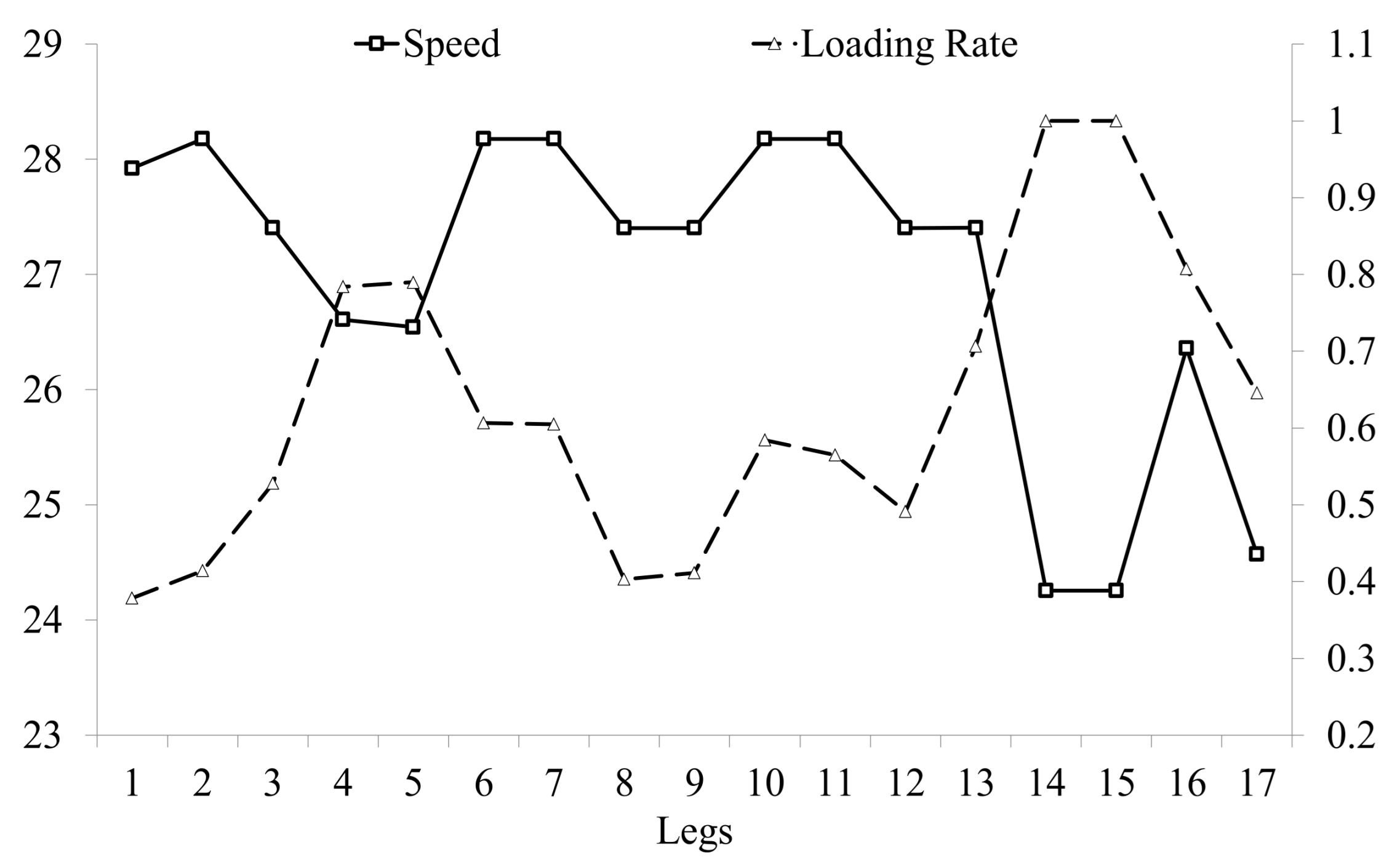
6.4. Analysis of the Relationship between Loading Rate and Sailing Speed

The optimal speed and loading rate of route 10 are selected as the research objects in order to study the relationship between loading rate and sailing speed and then get the following trend (Figure 5).
It can be seen from Figure 5 that there is a negative correlation between the optimal speed and the loading rate. With the increase of ship loading rate, the ship’s sailing speed will decrease; on the contrary, the ship’s loading rate will decrease, and the sailing speed will increase. It can be seen from the fuel consumption formula that the fuel consumption will increase with the increase of the ship’s payload or sailing speed. Hence, the increase of ship’s payload and the decrease of sailing speed can improve the energy conservation of ship operation.

7. Conclusions

In this paper, a speed optimization model is proposed for container ship fleet deployment to minimize the total operating costs and fuel consumption costs over the shipping network. Due to container transshipment, containers can be transported from origin port to destination port through many different routes. Although this provides flexibility for the operation of shipping companies, it brings challenges to the deployment of ship type and quantity.
From industry and practical perspectives, this study provides a multi-objective mixed-integer program that potentially can be applied to ship fleet deployment by decision-makers (e.g., the shipowner or the charterer) to reduce fuel consumption costs and operating costs. This paper serves as a valuable guide to determine the fleet deployment measures for liner shipping companies and make trade-offs among economic and environmental considerations.
The critical point of this paper is to balance operating costs and fuel consumption costs, which means that when studying the container ship fleet deployment, it is necessary to calculate fuel consumption according to on-ship payload and ship speed. On this basis, it can determine the ship’s fuel consumption more accurately by optimizing the speed of each leg to confirm the allocation of appropriate ship type and number for the route.
Numerical experiments were performed on 46 ports and 12 routes. Three important conclusions are summarized as follows. First, the number of segments within the range of ship’s payload is increased from 11 to 22, the average total cost is reduced 0.84%, and the average fuel consumption cost is reduced 4.41%. Thus, to obtain the more accurate solution, more piecewise numbers will be needed, but the calculating time will longer. Second, when the unit fuel consumption cost of the ship changes, the shipping company adopts “adding ship and slow down its speed” and “reducing ship and accelerate its speed” strategies to optimize the sailing speed. Third, from the analysis of the relationship between loading rate and sailing speed, it can be seen that there is a negative correlation between sailing speed and loading rate.
The research overview of this article is as follows: first, a mixed-integer nonlinear programming model is transformed into a mixed linear programming model through a series of linearization, taking the speed as the decision variable. Second, the calculation of bunker consumption is more scientific by considering the influence of ship’s payload and speed through nonlinear function. Third, the piecewise linear approximation algorithm is used to optimize the selection of segments on the premise of known accuracy so that the error of the calculation function can find a reasonable balance between the accuracy and the number of segments within a specific range. Under the condition of uncertain demand and speed change of each segment on the route, fleet deployment is the next research direction.

Author Contributions

Conceptualization and methodology, C.-F.G. and Z.-H.H.; writing—original draft preparation, C.-F.G.; writing—review and editing, Z.-H.H.; software, C.-F.G.; supervision, Z.-H.H. All authors have read and agreed to the published version of the manuscript.

Funding

This research was funded by the National Natural Science Foundation of China, grant number 71871136.

Institutional Review Board Statement

Not applicable.

Informed Consent Statement

Not applicable.

Data Availability Statement

Not applicable.

Acknowledgments

The authors gratefully acknowledge the editors and anonymous reviewers for their valuable comments that helped improve this paper. This study is partially supported by the National Nature Science of China (71871136).

Conflicts of Interest

The authors declare no conflict of interest.

References

  1. Wang, S.; Zhuge, D.; Zhen, L.; Lee, C.-Y. Liner Shipping Service Planning Under Sulfur Emission Regulations. Transp. Sci. 2021, 55, 491–509. [Google Scholar] [CrossRef]
  2. Beşikçi, E.B.; Arslan, O.; Turan, O.; Ölçe, A.I.R. An artificial neural network based decision support system for energy efficient ship operations. Comput. Oper. Res. 2016, 66, 393–401. [Google Scholar] [CrossRef] [Green Version]
  3. Yang, L.; Chen, G.; Zhao, J.; Rytter, N.G.M. Ship Speed Optimization Considering Ocean Currents to Enhance Environmental Sustainability in Maritime Shipping. Sustainability 2020, 12, 3649. [Google Scholar] [CrossRef]
  4. Wen, M.; Pacino, D.; Kontovas, C.A.; Psaraftis, H.N. A multiple ship routing and speed optimization problem under time, cost and environmental objectives. Transp. Res. Part D Transp. Environ. 2017, 52, 303–321. [Google Scholar] [CrossRef]
  5. Acciaro, M. Real option analysis for environmental compliance: LNG and emission control areas. Transp. Res. Part D Transp. Environ. 2014, 28, 41–50. [Google Scholar] [CrossRef]
  6. Coraddu, A.; Oneto, L.; Baldi, F.; Anguita, D. Vessels fuel consumption forecast and trim optimisation: A data analytics perspective. Ocean Eng. 2017, 130, 351–370. [Google Scholar] [CrossRef]
  7. Psaraftis, H. Speed Optimization vs Speed Reduction: The Choice between Speed Limits and a Bunker Levy. Sustainability 2019, 11, 2249. [Google Scholar] [CrossRef] [Green Version]
  8. Christiansen, M.; Fagerholta, K.; Nygreen, B.; Ronenc, D. Ship routing and scheduling in the new millennium. Eur. J. Oper. Res. 2013, 228, 467–483. [Google Scholar] [CrossRef]
  9. Jaramillo, D.I.; Perakis, A.N. Fleet deployment optimization for liner shipping Part Implementation and results. Marit. Policy Manag. 1991, 18, 235–262. [Google Scholar] [CrossRef]
  10. Gelareh, S.; Pisinger, D. Fleet deployment, network design and hub location of liner shipping companies. Transp. Res. Part E Logist. Transp. Rev. 2011, 47, 947–964. [Google Scholar] [CrossRef]
  11. Wang, S.; Meng, Q. Liner ship fleet deployment with container transshipment operations. Transp. Res. Part E Logist. Transp. Rev. 2012, 48, 470–484. [Google Scholar] [CrossRef]
  12. Chandra, S.; Christiansen, M.; Fagerholt, K. Combined fleet deployment and inventory management in roll-on/roll-off shipping. Transp. Res. Part E Logist. Transp. Rev. 2016, 92, 43–55. [Google Scholar] [CrossRef]
  13. Song, Y.; Yue, Y. Optimization Model of Fleet Deployment Plan of Liners. Procedia Eng. 2016, 137, 391–398. [Google Scholar] [CrossRef] [Green Version]
  14. Gelareh, S.; Meng, Q. A novel modeling approach for the fleet deployment problem within a short-term planning horizon. Transp. Res. Part E Logist. Transp. Rev. 2010, 46, 76–89. [Google Scholar] [CrossRef]
  15. Andersson, H.; Fagerholt, K.; Hobbesland, K. Integrated maritime fleet deployment and speed optimization: Case study from RoRo shipping. Comput. Oper. Res. 2015, 55, 233–240. [Google Scholar] [CrossRef]
  16. Wang, X.; Fagerholt, K.; Wallace, S.W. Planning for charters: A stochastic maritime fleet composition and deployment problem. Omega 2018, 79, 54–66. [Google Scholar] [CrossRef] [Green Version]
  17. Zhen, L.; Hu, Y.; Wang, S.; Laporte, G.; Wu, Y. Fleet deployment and demand fulfillment for container shipping liners. Transp. Res. Part B Methodol. 2019, 120, 15–32. [Google Scholar] [CrossRef]
  18. Norstad, I.; Fagerholt, K.; Laporte, G. Tramp ship routing and scheduling with speed optimization. Transp. Res. Part C Emerg. Technol. 2011, 19, 853–865. [Google Scholar] [CrossRef]
  19. Zacharioudakis, P.G.; Iordanis, S.; Lyridis, D.V.; Psaraftis, H.N. Liner shipping cycle cost modelling, fleet deployment optimization and what-if analysis. Marit. Econ. Logist. 2011, 13, 278–297. [Google Scholar] [CrossRef]
  20. Du, Y.; Qiang, M.; Shuaian, W.; Haibod, K. Two-phase optimal solutions for ship speed and trim optimization over a voyage using voyage report data. Transp. Res. Part B Methodol. 2019, 122, 88–114. [Google Scholar] [CrossRef]
  21. Ronen, D. The effect of oil price on containership speed and fleet size. J. Oper. Res. Soc. 2011, 62, 211–216. [Google Scholar] [CrossRef]
  22. Wang, S.; Meng, Q. Sailing speed optimization for container ships in a liner shipping network. Transp. Res. Part E Logist. Transp. Rev. 2012, 48, 701–714. [Google Scholar] [CrossRef]
  23. Gkonis, K.G.; Psaraftis, H.N. Modeling tankers’ optimal speed and emissions. Soc. Nav. Archit. Mar. Eng. Trans. 2012, 120, 90–115. [Google Scholar]
  24. Psaraftis, H.N.; Kontovas, C.A. Ship speed optimization: Concepts, models and combined speed-routing scenarios. Transp. Res. Part C Emerg. Technol. 2014, 44, 52–69. [Google Scholar] [CrossRef] [Green Version]
  25. Xia, J.; Li, K.X.; Ma, H.; Xu, Z. Joint Planning of Fleet Deployment, Speed Optimization, and Cargo Allocation for Liner Shipping. Transp. Sci. 2015, 49, 922–938. [Google Scholar] [CrossRef]
  26. Wang, Y.; Meng, Q.; Du, Y. Liner container seasonal shipping revenue management. Transp. Res. Part B Methodol. 2015, 82, 141–161. [Google Scholar] [CrossRef]
  27. Al-Khayyal, F.A.; Falk, J.E. Jointly Constrained Biconvex Programming. Math. Oper. Res. 1983, 8, 273–286. [Google Scholar] [CrossRef]
  28. Yang, H.; Xing, Y. Containerships Sailing Speed and Fleet Deployment Optimization under a Time-Based Differentiated Freight Rate Strategy. J. Adv. Transp. 2020, 2020, 1–16. [Google Scholar] [CrossRef]
Figure 1. Shipping network of composition by three routes.
Sustainability 13 05242 g001
Figure 2. The linear outer-approximation technique.
Sustainability 13 05242 g002
Figure 3. Improved piecewise linear approximation algorithm flow.
Sustainability 13 05242 g003
Figure 4. The piecewise linear function to approximate.
Sustainability 13 05242 g004
Figure 5. Relationship between sailing speed and loading rate of each leg of route 10.
Sustainability 13 05242 g005
Table 1. Description of symbols.
SetsDescription
R Ship   routes   set   r R
P Ports set p , o , d P
V Ship   types   v V
Parameters
V r Candidate   ship   types   set   of   route   r
I r Port   indices   for   route   r
P r , i The ith port of call
I r , p Port   p   indices   of   route   r   p P , I r , p I r
R p Routes   set   of   berthing   port   p
C p t r a n Unit container transshipment cost
C p l o a d Unit   loading   cos t   at   port   p
C p d i s c Unit   discharge   cos t   at   port   p
D o , d Transport   demand   between   port   o   and   port     d
C v o p r Fixed   cos ts   of   operating   a   ship   of   type   v
C p , v b e r Unit   cos t   of   berthing   operation   at   port   p   for   ship   of   type   v
Q v Ship   of   type   v capacity
C v o u t Chartering - out   profit   of   type   v ship
C r , v f i x Costs related to the voyage
T p , v c o n t Per - container   operating   time   at   port   p   for   ship   type   v
Decision Variables
n v i n Number   of   ships   of   type   v   charted   for   the   number   of   type   v ships
n v o u t Chartering - out   number   of   type   v ships
m r , v Number   of   type   v   ships   deployed   on   ship   route   r
z r , v , i Number   of   containers   handled   for   a   ship   of   type   v   at   the   ith   port   of   call   on   ship   route   r
x r , v 1 ,   if   deployed   ships   of   type   v   on   route   r , and 0 otherwise
z o , r , i l o a d Number   of   containers   loaded   at   the   i - th   port   of   call   on   route   r   originating   from   port   o
z o , r , i d i s c Number   of   containers   discharged   at   the   i - th   port   of   call   on   route   r   originating from port o
z o , r , i f l o w Number   of   containers   originating   from   port   o   sailing   on   the   ith   leg   of   route   r
z p t r a n Number   of   containers   transshipped   at   a   particular   port   p
e r , i Ballast water weight required for ship stability sailing on the i-th leg of route r
s r i Sailing   speed   during   leg   i   of   route   r
w r i Ship   payload   during   leg   i   of   route   r
Table 2. Basic ship parameters.
Ship Type
SmallMediumLargeGiant
Capacity of different types of ships Q v (TEU)15003000500010,000
Fixed operating costs of different types of ships C v o p r (week)51,92376,923115,384173,076
Unit cost of berthing operation of different types of ships C p , v b e r   (h)500100016663333
Per-container operating time of different types of ships T p , v c o n t (h)0.0250.0120.0110.008
Number of ships owned by the shipping lines N v o w n 20202020
Chartering-out profit of different types of ships C v o u t 52,50077,00098,000140,000
Chartering-in cost of different types of ships C v i n 66,50094,500122,500175,000
Table 3. Parameters related to the 12 ship routes.
No.Ports Corresponding Number, Ports Order (Distance between Ports)
11Yokohama (15)     2Tokyo (177)     3Nagoya (201)     4Kobe (734)     5Shanghai (745)     6Hong Kong (1568) 1Yokohama
27Ho Chi Minh (589)     8Laem Chabang (755)     9Singapore (187)     10Port Klang (830)   7Ho Chi Minh
311Brisbane (419)     12Sydney (512)     13Melbourne (470)     14Adelaide (1325)     15Fremantle (1733)     16Jakarta (483)     9Singapore (3649)     11Brisbane
417Manila (527)   18Kaohsiung (164)     19Xiamen (260)   6Hong Kong (15)     20Yantian (19)     21Chiwan (17)     6Hong Kong (620)     17Manila
522Dalian (187)     23Xingang (379)     24Qingdao (303)     5Shanghai (93)     25Ningbo (93)     5Shanghai (383)     26Kwangyang (72)     27Busan (487)     22Dalian
628Chittagong (872)     29Chennai (573)     30Colombo (306)     31Cochin (723)     32Nhava Sheva (723)     31Cochin (306)   30Colombo (573)     29Chennai (872)     28Chittagong
733Sokhna (265)     34Aqabah (554)     35Jeddah (1268)     36Salalah (885)     37Karachi (688)   38Jebel Ali (862)     36Salalah (1878)     33Sokhna
839Southampton (165)     40Thamesport (386)     41Hamburg (82)   42Bremerhaven (196)     43Rotterdam (42)     44Antwerp (51)     45Zeebrugge (168)     46Le Havre (103)     39Southampton
910Port Klang (187)     9Singapore (483)     16Jakarta (1917)     18Kaohsiung (904)     27Busan (904)   18Kaohsiung (342)   6Hong Kong (17)   21Chiwan (1597)   10Port Klang
1039Southampton (3162)     33Sokhna (1878)     36Salalah (1643)     30Colombo (1560)     9Singapore (1415)     6Hong Kong (260)   19Xiamen (486)     5Shanghai (448)     27Busan (487)     22Dalian (187)     23Xingang (379)     24Qingdao (303)   5Shanghai (745)     6Hong Kong (1415)     9Singapore (1560)     30Colombo (1643)     36Salalah (5029)     39Southampton
1111Brisbane (419)   12Sydney (512)   13Melbourne (470)   14Adelaide (1325)   15Fremantle (3148)   30Colombo (1643)   36Salalah (5244)   43Rotterdam (5244)   36Salalah (1643)   30Colombo (5191)   11Brisbane
1220Yantian (9956)     41Hamburg (3621)   33Sokhna (620)     35Jeddah (4156)   10Port Klang (187)   9Singapore (1309)     17Manila (629)   20Yantian
Table 4. The ship-fixed operating costs of 12 ship routes.
c r , v f Ship Type Ship Type
No.SmallMediumLargeGiantNo.SmallMediumLargeGiant
1226,198280,542404,0007404,711499,139710,000
2154,791191,900276,1008129,712149,622199,300
3533,980656,891929,1009501,088551,946715,100
4155,123176,013232,200101,883,0072,430,000
5148,807187,600279,700111,504,2311,843,1782,583,900
6322,916400,072574,800121,235,3131,512,7552,117,800
Table 5. Four scenarios composed of the different approximation error ε 1 and ε 2 combinations.
ε 1 Segments ε 2 SegmentsScenario 1Scenario 2Scenario 3Scenario 4
1.6 × 10−3687.6 × 10−3116868135135
4.2 × 10−41359.6 × 10−42211221122
Table 6. Various cost comparisons of fleet deployment under different scenarios.
β Scenario 1Scenario 2 Δ 1 × 10 2 Δ 2 × 10 2
f × 10 7 f F C × 10 6 f C T × 10 6 GapTime f × 10 7 f F C × 10 6 f C T × 10 6 GapTime
1002.263451.4568985.42274.5785%157s2.251791.3050535.42274.1103%1320s−0.5−1.0
2002.383972.2911485.40824.7686%131s2.373632.2033965.40824.7209%1693s−0.4−3.8
3002.505882.9785365.3974.3182%116s2.47362.7576975.3974.7709%1455s−1.2−7.4
4002.611243.1534225.39574.9317%132s2.553962.9240085.39574.3785%1791s−2.1−7.2
5002.657453.4702095.35624.9863%170s2.676373.7808555.35624.7166%1422s−0.78.9
6002.719383.7258775.45094.8223%176s2.69143.6867785.45094.7034%1534s−1.0−1.0
β Scenario 3Scenario 4 Δ 3 × 10 2 Δ 4 × 10 2
f × 10 7 f F C × 10 6 f C T × 10 6 GapTime f × 10 7 f F C × 10 6 f C T × 10 6 GapTime
1002.257751.534765.42084.2802%219s2.25471.2856475.39084.4730%1663s−0.1−16
2002.390832.2304195.37244.8466%182s2.373662.2085085.32394.6335%1807s−0.7−0.9
3002.508713.1461335.4089994.7001%160s2.473032.5895135.3524.9580%2006s−1.4−18
4002.593373.2047965.34494.7656%146s2.564883.0679225.37264.8849%1514s−1.1−4.2
5002.666133.5968155.35614.9071%159s2.641553.5361235.36424.9157%1514s−0.9−1.6
6002.69163.7048315.3462994.8691%167s2.690723.6778275.36194.8956%1606s−0.0−0.7
Notes: Δ 1 = f S c e n a r i o 2 f S c e n a r i o 1 / f S c e n a r i o 1 ,   Δ 2 = f S c e n a r i o 2 F C f S c e n a r i o 1 F C / f S c e n a r i o 1 F C , Δ 3 = f S c e n a r i o 4 f S c e n a r i o 3 / f S c e n a r i o 3 , Δ 4 = f S c e n a r i o 4 F C f S c e n a r i o 3 F C / f S c e n a r i o 3 F C , G a p = B P B F / B P .
Table 7. Ship deployment and sailing speed changes of Route 2 and Route 6.
β Ship DeploymentEach Legs Speed of Route 2Ship DeploymentEach Legs Speed of Route 6
TypeNum1234TypeNum12345678
1003000125.9825.6225.9823.831500316.2616.0016.0016.2616.2116.2616.2624.45
2001500210.3610.4210.3623.833000221.0620.6220.6220.8920.6220.6220.6224.45
3003000125.5125.9825.9823.833000220.6221.0620.6220.8920.6221.0620.6224.45
4001500210.4110.3610.4723.833000221.0620.6220.6220.6220.7121.0620.6224.45
5003000125.5125.9825.9823.831500316.26 16.0716.0016.2616.2616.0016.2624.45
6001500210.5810.6110.5823.831500311.2411.1711.1711.1711.1711.1711.1724.45
Publisher’s Note: MDPI stays neutral with regard to jurisdictional claims in published maps and institutional affiliations.

