Reactive UAV Fleet’s Mission Planning in Highly Dynamic and Unpredictable Environments

Abstract

Unmanned aerial vehicles (UAVs) create an interesting alternative for establishing more sustainable urban freight deliveries. The substitution of traditional trucks in the last-mile distribution by a UAV fleet can contribute to urban sustainability by reducing air pollution and increasing urban freight efficiency. This paper presents a novel approach to the joint proactive and reactive planning of deliveries by a UAV fleet. We develop a receding horizon-based approach to reactive, online planning for the UAV fleet’s mission. We considered the delivery of goods to spatially dispersed customers over an assumed time horizon. Forecasted weather changes affect the energy consumption of UAVs and limit their range. Therefore, consideration should be given to plans for follow-up tasks, previously unmet needs, and predictions of disturbances over a moving time horizon. We propose a set of reaction rules that can be encountered during delivery in a highly dynamic and unpredictable environment. We implement a constraint programming paradigm, which is well suited to cope with the nonlinearity of the system’s characteristics. The proposed approach to online reactive UAV routing is evaluated in several instances. The computational experiments have shown that the developed model is capable of providing feasible plans for a UAV fleet’s mission that are robust to changes in weather and customer’s orders.

1. Introduction

Delivering goods in urban areas is related to negative externalities, such as congestion, noise, and air pollution. Urban distribution operations have a significant impact on three dimensions of sustainability (economic, environmental, and social) [1].

In the framework of city logistics, the general issues related to urban freight deliveries (in the framework of city logistics) are identified in [2,3,4] as follows:

• Higher costs for urban goods delivery.
• Nuisance including traffic congestion and crashes.
• Green House Gas (GHG) emissions and local emissions.
• Reduction of the greenfield sites and open spaces (due to the transport infrastructure development).
• Increasing amounts of waste products, such as tires, oil, and other waste products related to maintenance of traditional delivery and transport systems.
• Noise and vibration.

In the European Union, over 75% of the population lives in cities. The growing urban population is linked to the higher demand for deliveries in urban areas. Freight transport in urban areas generates 25% of emissions of CO₂ in a city (EC UTF, 2012). Due to the organization of traffic in the city structure, in urban freights there are more frequent stops and shorter distances traveled. For that reason, urban freight transport pollutes air more than long-distance transport [5]. The city logistics issues involve different stakeholders like local authorities, residents, consumers, visitors to the city, shippers, receivers, transport companies, and public transport operators [6,7]. In this paper, we take into consideration the shippers and receivers. Due to the development of e-commerce, a considerable share of deliveries is made directly to individual customers [4]. The “last-mile” of delivery is performed in highly urbanized areas, where the use of traditional trucks is not effective [8]. The negative effects of goods deliveries in urban areas are caused mainly by a low level of cooperation between partners in the supply chain, and also the low effectiveness of transport systems [9]. The low efficiency of the last-mile operations (with the use of traditional trucks) results from a spatial distribution of relatively small receiving points, demands for more frequent but smaller shipments, various delivery time windows, and changes in the delivery schedules due to the absence of the recipient. This inefficiency is translated into ecological concerns and actions are taken on a local, regional, and national, as well as cross-boundary, scale to limit the negative impacts of urban freight deliveries on the environment [9]. Moreover, the share of “last-mile deliveries” increases due to e-commerce. There is a need for innovative types of deliveries in inner cities, reducing the negative ecological and social impact of transport. A lot of attention has been also given to the use of alternative fuel vehicles in urban logistics, in particular, the usability of electric freight vehicles (EFVs) [8] and zero-emissions solutions [10,11]. To address these issues, several innovative solutions have been proposed such as [12]: Information and Communication Technologies (ICT), Intelligent Transport Systems (ITS), Internet of Things (IoT), Artificial Intelligence (AI), and deliveries with robots (e.g., UAVs).

Public authorities have taken action to encourage the use of green vehicles in the last mile of logistics [13]. Unmanned aerial vehicles (UAVs) create an interesting alternative for decarbonizing transport, reducing air pollution, and increasing urban freight efficiency [14,15,16]. Compared with delivery trucks [17], UAVs consume less energy per package kilometer. The current scale of the applications of UAVs in urban distribution is relatively low [13,18]. Urban deliveries are characterized by frequent stop-and-go movements, low consolidation, and frequent rescheduling (e.g., due to the cancelation of delivery or absence of recipient) [13]. The use of UAVs on a larger scale requires research to provide better solutions to meet the challenges related to dynamic changing conditions [19,20,21].

In this paper, we consider the reactive planning of a UAV fleet’s mission problem with highly dynamic and unpredictable environment constraints. Typical disruptions in urban deliveries by UAVs may be caused by changes in the order by customers or changing weather conditions (e.g., a sharp drop in temperature, icing of propellers, turbulences), which affect the energy consumption of UAVs and cause them to have a shorter range due to the depletion of batteries [22,23]. For that reason, the routing of a UAV fleet in a partially known and unpredictable environment should guarantee a reactive online determined contingency reaction.

Path planning for UAVs has been an active research area, and the existing scientific approaches can be classified as:

• optimization criteria (e.g., fuel consumption [24], delivery time [25], delivery costs [26])
• fields of application (e.g., reconnaissance and mapping [27], package delivery [28], delivery communication capabilities [29,30])
• Fleet planning and scheduling (e.g., congestion-free scheduling [23,31,32], fleet assignment [33]).

The aim of UAV fleet mission planning is to find a sequence of waypoints that connect the starting point to the destination location for every vehicle in the fleet. UAV routes can be determined through proactive planning [34], and generated in offline mode or in reactive planning [35,36,37], while executed in the online mode. Routes determined in proactive planning guarantee the achievement of the planned mission’s goal for the environment’s parameters, which change in predetermined intervals. Sometimes the routes determined in proactive planning cannot guarantee the achievement of the mission goal. That issue happens because scenarios corresponding to planned reactive rules do not guarantee the existence of reactive end-to-end paths employed in the routing process [37] while adapting it to changes in the environment during mission execution.

Usually, the designed mission plans are analyzed from multiple perspectives including changing weather conditions (i.e., wind speed and direction), payload and energy capacities of UAVs, fleet sizes, the number of delivery points visited by a UAV on a mission, and delivery performance [23,31,38,39,40,41,42]. Due to the NP-hard nature of the considered problems, the models used in the above-mentioned contexts include representations implementing formalisms of MLP [43,44], declarative modelling [22,31,34,45], computer simulation [46,47], AI [48], and heuristic searching [49].

Relatively few works devoted to the planning of UAV fleet missions take into account the various technical and environmental factors influencing possible solutions [22]. Among the listed factors, the following are significant:

• Technical parameters of UAVs (UAV dimensions, battery capacity, and carrying payload limit).
• Changing weather conditions (the wind speed, wind direction, wind gust, precipitation, icing, turbulence, and air density and temperature).
• Dynamically changing terms of delivery and static or moving obstacles (withdrawing or changing the date and place of deliveries as well as their volume, and collision avoidance).

Those conditions, by influencing the battery consumption, determine the range of the planned missions. The time of completion of the UAV’s mission is normally calculated offline by using information about the known route length and the parameters of the employed vehicle. However, studies on the influence of weather-dependent energy consumption constraints, and changes in the weight of the shipment, as well as changes in weather conditions determining energy consumptions, are rare [22,50].

In this context, a research gap concerns both the dynamic control [51,52] and the proactive planning [35,36,39] of UAV missions. Dynamic control policies are responsible for carrying out all of the real-time operational functions required to maneuver a vehicle. Reactive routing strategies allow for responses after an incident occurrence. They both play a pivotal role in a vehicle’s navigation in uncertain operational environments. The reactive routing strategies linking the “route discovery” (proactive route planning) and “route maintenance” (reactive rules adopting) concepts [53] are especially responsible for the UAV’s robustness to the changes that appear in the urban distribution context. The reactive routing strategies match the needs of dynamically developing vehicular ad hoc networks (VANETs), which are characterized by frequent path failures due to the high mobility caused by the sudden changes of vehicle direction [54,55].

The indicated research gap has become the inspiration for conducting this research, which focuses on reactive planning of deliveries by UAV fleets that are resistant to sudden changes in weather conditions and unforeseen changes in the delivery schedules.

The research problem concerns the delivery of goods within assumed time windows to a set of spatially dispersed customers, over a given time horizon. When forecasted changes in the weather affect the energy consumption of UAVs and limit their range, then some of the demand is unmet. Proactive planning of subsequent missions will take into account previously unmet demand as well as predictions of future disturbances over a moving time horizon. Therefore, we aim to propose a set of condition-action (if-then) rules for situations that can be encountered in the course of delivery missions in a highly dynamic and unpredictable environment.

The originality of this paper results from merging the proactive and reactive planning of the missions of UAV fleets. The developed model allows for predictive (i.e., taking into account forecasted weather conditions changing) and reactive (i.e., enabling interruption of a drone’s mission) planning of delivery missions in terms of the Constraint Satisfaction Problem easily implemented in a commercially available constraint programming environment, e.g., IBM ILOG.

The paper is structured as follows. The research problem and methods are presented in Section 2. The declarative model for reactive planning of deliveries by a UAV fleet using the Constraint Satisfaction Problem is described. Computational experiments are presented in Section 3. The discussion on results is presented in Section 4. The final conclusions are stated in Section 5, followed by a description of future research.

2. Materials and Methods

Most approaches to this topic employ either proactive or reactive route planning strategies. Proactive planning allows for the selection of a set of waypoints that avoids the anticipated disturbances [34]. In reactive planning (instead of an actions’ specific sequence) sets of condition-actions, or if-then rules (corresponding to possible situations that may appear), are prepared. In that context, reactive planning is a process in which one rule is selected (from available rules assigned to the relevant situation) in order to implement the required contingency actions [56,57].

This research addresses the existing gap in the state-of-the-art of mission planning, with regard to the changing weather conditions and uncertainty of unpredictable behavior of the ordering party. We search for a feasible plan for a UAV fleet’s mission that allows for successful completion of the deliveries before the UAV’s battery discharging. Such a plan will be robust to disturbances relating to the changes in weather conditions and the customer’s order (e.g., the recipient is absent or cancels the delivery). We have given:

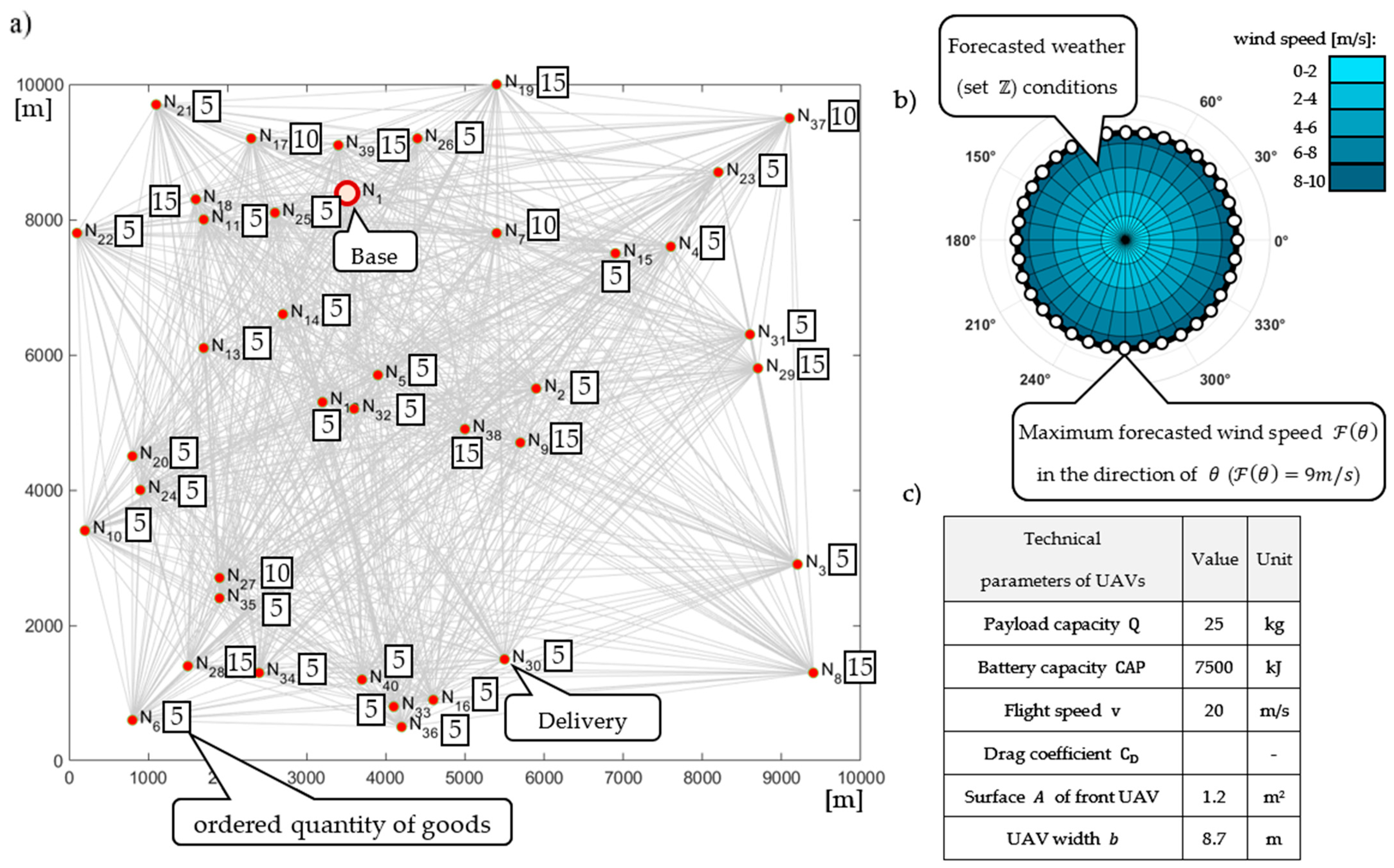
• A set of spatially dispersed delivery points
• A fleet of capacitated UAVs
• A distribution network with distinguished, so-called base nodes, used for loading UAVs and replacing used batteries, as well as a set of edges labeled by travel times linking adjacent nodes.

We have also given disturbances including types of order changes and the weather forecast for the given time horizon.

Our research problem is to find the proactive plan for the UAV fleet’s mission that ensures completion of the assumed deliveries in a given time horizon. That plan is determined by the forecasted changes in weather conditions. The feasible mission plan consists of a sequence of overlapping sub-missions (covering the UAV’s routes and flight schedule). The time and range of sub-missions are limited by the battery’s capacity and its current depletion rate. We also search for a reactive plan with a set of condition-action rules that defines which type of contingency operations will be taken when disturbances appear. A disturbance can be related to a change in the size and location of delivery and/or dynamic changes in weather conditions (exceeding forecasted weather conditions). Then, for the designated UAV’s baseline routes and a set of rules, the reactive online delivery plan is implemented. The joint proactive and reactive planning allows for changes to be made during the execution of the initial plans. When, at a given waypoint, a disturbance appears related to at least one condition among the assigned reactive rules, then the corresponding initial (proactively planned) UAV’s delivery is properly rerouted.

The mathematical formulation of this problem belongs to the class of NP-hard problems [33,38,50,58], as it consists of many highly nonlinear constraints. Those constraints are related to energy consumption under the different directions and speed of the wind and variable loads. Therefore, a declarative reference model is applied [13]. Our contribution extends the previous works [22,23,31,34], which have explored the proactive planning methods for fast prototyping of feasible UAV fleet routing, in regard to the changing weather conditions. In the next sections, we present the stages of our model development.

2.1. General Concept—The Method for Online Routing

We consider a distribution network, that is modeled by the graph $G=\left(N,E\right)$ where $N=\left\{N_1,\dots ,N_{\lambda },\dots ,N_n\right\}$ signifies the set of $n=\left|N\right|$ nodes (distinguishing $N_1$ node representing a base and $\left\{N_2,\dots ,N_n\right\}$ nodes representing delivery points), and $E=\left\{\left(N_i,N_j\right)| i, j \in \left\{1,\dots ,n\right\},i \ne j\right\}$ signifies the set of edges determining the possible connections between nodes.

There is given a fleet of UAVs $\mathcal{U}=\left\{U_1,\dots ,U_k,\dots ,U_K\right\}$ that delivers to the points {$N_2,\dots ,N_n$}. It is assumed that to each delivery point $N_{\lambda }$ an ordered quantity of goods $z_{\lambda }\in \mathbb{N}$ kg (taken from the base $N_1$) should be transported. Deliveries are made as part of mission S, which consists of sub-missions ${}_{ }{}^{l}S$ (i.e., delivery plans that include a single course of UAVs: base-delivery points-based). $Z$ denotes a sequence consisting of variables $z_{\lambda }$: $Z$ $=(z_1,\dots ,z_n$). It is assumed that all required goods should be delivered in the given horizon time $H$. The number of goods delivered during one sub-mission ${}_{ }{}^{l}S$ by the $U_k$ to the delivery point $N_{\lambda }$ is determined by the variable ${}_{ }{}^{l}c{}_{\lambda }^k\in \mathbb{N}$ kg. ${}_{ }{}^{l}C$ is a sequence: ${}_{ }{}^{l}C=\left({}_{ }{}^{l}c{}_1^1,\dots ,{}_{ }{}^{l}c{}_1^K,\dots ,{}_{ }{}^{l}c{}_n^1,\dots ,{}_{ }{}^{l}c{}_n^K\right)$ determining the payload weight delivered by fleet $\mathcal{U}$. The sum of goods delivered to point $N_{\lambda }$ should be equal to the required value of $z_{\lambda }$ (${\displaystyle \sum }_{l=1}^L{\displaystyle \sum }_{k=1}^K{}_{ }{}^{l}c{}_{\lambda }^k=z_{\lambda }$, where: $L$ denotes the number of sub-missions ${}_{ }{}^{l}S$). It is assumed that each delivery point can be serviced by several UAVs. In addition, a UAV used in a sub-mission can service several delivery points. Variable $Q_k$ denotes the payload capacity of $U_k$ kg (amount of goods transported by $U_k$ cannot exceed $Q_k$). Moreover, each $U_k$ is described by technical parameters: battery capacity $CAP$, airspeed $va$, drag coefficient $C_D$, front surface $A$ of UAV, and UAV width $b$. The time spent on take-off and landing $U_k$ on delivery point $N_{\lambda }$ is indicated by variable $w_{\lambda }\in \mathbb{N}$ s.

Note that ${}_{ }{}^l\mathcal{U}\subseteq \mathcal{U}$ denotes a set of UAVs used during sub-mission ${}_{ }{}^{l}S$. The moment when the $U_k\in {}_{ }{}^l\mathcal{U}$ arrives at the delivery point $N_{\lambda }$ during sub-mission ${}_{ }{}^{l}S$ is indicated by variable ${}_{ }{}^{l}y{}_{\lambda }^k\in \mathbb{N}$[s]. In that context, the sequence ${}_{ }{}^{l}Y$ consisting of moments ${}_{ }{}^{l}y{}_{\lambda }^k$, is called the schedule of the fleet ${}_{ }{}^l\mathcal{U}$: ${}_{ }{}^{l}Y=\left({}_{ }{}^{l}y{}_1^1,\dots ,{}_{ }{}^{l}y{}_1^K,\dots ,{}_{ }{}^{l}y{}_n^1,\dots ,{}_{ }{}^{l}y{}_n^K\right)$.

We assume that the variable $t_{\beta ,\lambda }\in \mathbb{N}$[s] determines traveling time between nodes $N_{\beta }$,$N_{\lambda }$, where: $\left(N_{\beta },N_{\lambda }\right)\in E$ and routes of $U_k\in {}_{ }{}^l\mathcal{U}$ during sub-mission ${}_{ }{}^{l}S$ are represented by sequences: ${}_{ }{}^l\pi {}_k=\left(N_{k_1},\dots ,N_{k_i},N_{k_{i+1}},\dots ,N_{k_{\mu }}\right)$, where: $k_i\in \left\{1,\dots ,n\right\}$, $\left(N_{k_i},N_{k_{i+1}}\right)\in E$. ${}_{ }{}^l\Pi$ denotes a sequence of routes executed during sub-mission ${}_{ }{}^{l}S$: ${}_{ }{}^l\Pi =\left({}_{ }{}^l\pi {}_1,\dots ,{}_{ }{}^l\pi {}_k,\dots ,{}_{ }{}^l\pi {}_K\right)$ (in cases when $U_k\notin {}_{ }{}^l\mathcal{U}$ then ${}_{ }{}^l\pi {}_k=△$). The delivery plan of one UAV’s sub-mission ${}_{ }{}^{l}S$ is defined as a sequence: ${}_{ }{}^{l}S=\left({}_{ }{}^l\mathcal{U},{}_{ }{}^l\Pi ,{}_{ }{}^{l}Y,{}_{ }{}^{l}C\right)$.

It is assumed that a plan of sub-mission ${}_{ }{}^{l}S$ is implemented under specific weather conditions, i.e., the weather forecast is known for each sub-mission ${}_{ }{}^{l}S$. The forecasted weather conditions are described by the set $\mathbb{F}$ of pairs composed of direction $\theta$ and wind speed $\left(\theta ,vw\right)\in \mathcal{F}$, i.e., $\mathbb{F}$ is defined as follows: $\mathbb{F}=\left\{\left(\theta ,vw\right)|\theta \in \left[0°,360°\right),vw\in \left[0, ℱ\left(\theta \right)\right]\right\}$. Where $Z\left(\theta \right)$ is a function whose values determine the maximum forecasted wind speed for the given direction $\theta$. The weather conditions determine the admissibility of the adopted sub-mission’s plan ${}_{ }{}^{l}S$, i.e., they determine whether, during its implementation, the batteries of one of the UAVs will not be prematurely discharged.

A function ${{\rm Y}}_{k,l}\left(\theta \right)$ determines the borderline wind speed (for a given direction $\theta$), which guarantees the successful completion of the delivery plan by the $U_k$ during sub-mission ${}_{ }{}^{l}S$ in the distribution network $G$: ${{\rm Y}}_{k,l}\left(\theta \right)=\max {\Gamma }_{k,l}\left(\theta \right)$, where: ${\Gamma }_{k,l}\left(\theta \right)$–set of wind speed values $vw$ for a given direction $\theta$, for which the battery of $U_k$ is not discharged. The sub-mission’s plan ${}_{ }{}^{l}S$ is assumed [27] to be resistant to the forecast weather conditions $\mathbb{F}$ if the boundary wind ${{\rm Y}}_{k,l}\left(\theta \right)$ of all $U_k\in {}_{ }{}^l\mathcal{U}$ in any direction $\theta$ does not exceed the forecasted value $Z\left(\theta \right)$: ${\forall }_{U_k\in {}_{ }{}^l\mathcal{U}}{\forall }_{\theta \in \left[0°,360°\right)}{{\rm Y}}_{k,l}\left(\theta \right)\ge ℱ\left(\theta \right).$

A typical problem in proactively planning weatherproof missions is, as follows:

Does a route plan exist for mission $S$ (consisting of sub-missions ${}_{ }{}^{l}S$) of the fleet $\mathcal{U}$ that guarantees the delivery of the required goods to all recipients in the $G$ network in a given horizon $H$, and is resistant to the forecasted weather conditions $\mathbb{F}$ (${\forall }_{U_k\in {}_{ }{}^l\mathcal{U}}{\forall }_{\theta \in \left[0°,360°\right)}{{\rm Y}}_{k,l}\left(\theta \right)\ge ℱ\left(\theta \right)$?

In reality, however, the implementation of the designated mission S may be subject to various disturbances $IS$. Among them, there are sudden changes in the weather (beyond the expected ${ℱ}^{*}\left(\theta \right)$ range), and changes in orders $Z$), order changes (increase or decrease in the number of ordered deliveries $Z^{*}$), and changes in the number of delivery points served (changing the structure of the network $G^{*}$). The UAV fleet, when performing the delivery mission plan S, meets a disturbance $IS\left(t^{*}\right)$-covering one of the cases: the weather ${ℱ}^{*}\left(\theta \right)$, the network $G^{*}$, orders $Z^{*}$, at the time $t^{*}.$ In such situations, it becomes necessary to answer the following question:

Does a re-route plan exist for mission $S^{*}$ that guarantees the timely deliveries in a given time horizon $H$ and at acceptable battery levels?

A mission planning algorithm, which allows for the reactive routing of the UAV’s fleet with disturbances, is presented in the following subsections.

2.2. Reactive UAV Fleet Rerouting

To illustrate the motivation behind our approach, let us consider a distribution network from Figure 1a covering an area of 100 km² and containing 39 delivery points (nodes $N_2,\dots ,N_{40}$). The goods are delivered by the UAV fleet, which is stationed at the base $N_1$. The technical parameters of the UAVs are collected in Figure 1c. The weight of individual orders is:

$$\begin{array}{c}{z}_2=\dots =z_6=5\mathrm{kg},z_7=10\mathrm{kg},z_8=z_9=15\mathrm{kg},z_{10}=z_{11}=\dots =z_{16}\\ =5\mathrm{kg},z_{17}=10\mathrm{kg},z_{18}=z_{19}=15\mathrm{kg},z_{20}=\dots =z_{26}\\ =5\mathrm{kg},z_{27}=10\mathrm{kg},z_{28}=z_{29}=15\mathrm{kg},z_{30}=\dots =z_{36}\\ =5\mathrm{kg},z_{37}=10\mathrm{kg},z_{38}=z_{39}=15\mathrm{kg},z_{40}=5\mathrm{kg} \end{array}$$

In that context, we search for the minimum fleet size guaranteeing timely deliveries of the required amount of goods.

It is easy to notice that the smallest fleet that guarantees timely delivery (within the time horizon of 2.5 h) consists of $\mathcal{U}=\left\{U_1,U_2,U_3,U_4 \right\}$ UAVs, see Figure 2b. In turn, the fleet of $\mathcal{U}=\left\{U_1,U_2,U_3\right\}$ UAVs enables the realization of deliveries within the time horizon of 2.825 h. Figure 2a shows a schedule for carrying out transport operations (flight of the UAV between successive nodes) and unloading operations at subsequent collection points (landing in a node and unloading of goods) executed in the planned mission. In the case under consideration, mission $S$ consists of 6 sub-missions. Since only 3 UAVs were used, the delivery time to all delivery points (in given weather conditions see Figure 1) exceeds the allowable time limit of 2.5 h ($H=9000 \mathrm{s}$ ). It is possible to meet the set delivery date by using 4 UAVs: $\mathcal{U}=\left\{U_1,U_2,U_3,U_4\right\}$ ).

In this case, mission $S$ of Figure 2b consists of 6 sub-missions: $S=\left({}_{ }{}^{1}S,{}_{ }{}^{2}S,\dots ,{}_{ }{}^{6}S\right)$ (the wind speed does not exceed $9\frac{m}{s}$ ). In turn, Figure 2c illustrates the UAV routes occurring in sub-mission ${}_{ }{}^{1}S$ and executed due to resistance functions: ${{\rm Y}}_{1,1}\left(\theta \right)$, ${{\rm Y}}_{2,1}\left(\theta \right)$, ${{\rm Y}}_{3,1}\left(\theta \right)$, ${{\rm Y}}_{4,1}\left(\theta \right)$.

It is apparent that the following routes in mission ${}_{ }{}^{1}S$ are weatherproof for the given forecasted weather (i.e., ${{\rm Y}}_{k,l}\left(\theta \right)\ge ℱ\left(\theta \right)):$

$${}_{ }{}^1\mathsf{\pi }{}_1^{ }=\left(N_1,{ N}_{33},{ N}_{34},N_{13},N_{35},{ N}_{24},N_1\right); {}_{ }{}^1\mathsf{\pi }{}_2^{ }=\left(N_1,N_{31},N_{21},N_{22},N_{25},N_{26},N_1\right):$$

$${}_{ }{}^1\mathsf{\pi }{}_3^{ }=\left(N_1,N_{20},N_{10},N_{40},N_3,N_{14},N_1\right); {}_{ }{}^1\mathsf{\pi }{}_4^{ }=\left(N_1,N_{11},N_5,N_{12},N_{32},N_4,N_1\right)$$

and robustness function UAVs: ${{\rm Y}}_{1,1}\left(\theta \right)$, ${{\rm Y}}_{2,1}\left(\theta \right)$,${{\rm Y}}_{3,1}\left(\theta \right)$,${{\rm Y}}_{4,1}\left(\theta \right)$.

The mission under consideration is determined in the proactive planning process. In the course of carrying out a planned mission, many different disturbances can occur. However, other disturbances $IS$ including changes in weather or the appearance of a newly notified unplanned (not included in the planned route) order may occur in the course of mission execution.

All goods should be delivered within 2.5 h ($T=9000 \mathrm{s})$. The deliveries take place in different forecasted weather conditions (set $\mathbb{F}$), which are illustrated in Figure 1b. According to the forecast, the wind speed does not exceed $vw=9\frac{m}{s}$.

We consider a situation in which the weather conditions of the mission carried out rapidly changed at the time $t^{*}=3000 \mathrm{s}$, i.e., during the execution of sub-mission ${}_{ }{}^{2}S$, the wind speed increased to $vw=11\frac{m}{s}$ for direction $\theta =210°–230°$. Such a change means that this mission cannot be continued due to too much energy consumption (the mission’s resistance function ${{\rm Y}}_{3,2}\left(\theta \right)$ values are below the level corresponding to speed $11\frac{m}{s}$, see Figure 3. Figure 3 shows the location of the UAVs at time $t^{*}=3000 \mathrm{s}$, i.e., upon receipt of information about a change in weather, and marked the place where the battery $U_3$ will be discharged in the event of continuation of deliveries in accordance with the current plan ${}_{ }{}^{2}S$.

In this situation, it is necessary to correct the route of sub-mission ${}_{ }{}^{2}S$ being carried out, which forces the search for an answer to the following question:

Given a fleet $\mathcal{U}=\left\{U_1,U_2,U_3,U_4 \right\}$ providing deliveries to the delivery points allocated in the network $G$ from Figure 1. The fleet realizes the delivery mission plan $S^{*}$ from Figure 2b. At the time $t^{*}=3000$, a rapid weather ${ℱ}^{*}\left(\theta \right)$ change, i.e., disturbance $IS$, occurs, resulting in $vw=11\frac{m}{s}$; $\theta =210°–230°$.

Does a re-route plan exist for mission $S^{*}$ that guarantees the timely delivery of the ordered supplies in a given time horizon $H=9000 \mathrm{s}$ and at acceptable battery levels?

A procedure enabling a reactive (dynamic) planning of the mission for the UAV fleet in the event of a disturbance occurrence is presented in the next sections.

2.3. CSP Formulation

2.3.1. Reactive Mission Planning

The proposed reaction to the occurrence of a disturbance $IS\left(t^{*}\right)$ can be reduced to dynamic re-routing and rescheduling of previously adopted routes ${}_{ }{}^l\Pi$, schedules ${}_{ }{}^{l}Y$, and delivered goods ${}_{ }{}^{l}C$ stated in the basic proactive plan for the mission by the UAV fleet. It is a feasible adjustment of assumed ${}_{ }{}^l\Pi$, ${}_{ }{}^{l}Y$, and ${}_{ }{}^{l}C$ values to the changes in forecasted weather ${ℱ}^{*}\left(\theta \right)$, as well as corrections introduced to the network $G^{*}$ or orders $Z^{*}$.

To formally define the concept of disturbance $IS\left(t^{*}\right),$ let us introduce the concept of the state of mission implementation $S$. The state of mission $S$ at the time $t$ is defined as follows:

$$IS\left(t\right)=\left(M\left(t\right), {ℱ}^{*}\left(\theta ,t\right),{}_{ }{}^{*}G\left(t\right),Z^{*}\left(t\right)\right)$$

(1)

where:

$M\left(t\right)$ is an allocation of UAVs to nodes at the time $t$: ${}_{ }{}^{ }M\left(t\right)=\left(N_{a_1},\dots ,N_{a_k},\dots ,N_{a_K}\right)$, where: $a_k\in \left\{1,\dots ,n\right\}$ determines the (delivery points) node $N_{a_k}$ occupied by $U_k$ (or the node the $U_k$ is headed to),

${ℱ}^{*}\left(\theta ,t\right)$ is the weather condition forecast at the time $t$,

${}_{ }{}^{*}G\left(t\right)$ is the graph model of the distribution network structure at time t (number and location of delivery points), and

$Z^{*}\left(t\right)$ is the sequence of goods requested at the time $t$.

The state $IS\left(t^{*}\right)$ following condition $\left[{ℱ}^{*}\left(\theta ,t^{*}\right)\ne {ℱ}^{*}\left(\theta \right)\right]\vee \left[{}_{ }{}^{*}G\left(t^{*}\right)\ne G\right]\vee \left[Z^{*}\left(t^{*}\right)\ne Z\right]$ is called the disturbance occurring at the time $t^{*}$.

Occurrence of $IS\left(t^{*}\right)$ disturbance should be assessed in terms of its impact on the further course of the mission of S (that is, whether the value of the resistance function ${{\rm Y}}_{k,l}\left(\theta \right)$ is greater than $ℱ\left(\theta \right)$). If the implementation of the mission is at risk (${{\rm Y}}_{k,l}\left(\theta \right)\ngeqq ℱ\left(\theta \right)$), an attempt should be made to reschedule it. The following condition action (if-then) rules are used for this purpose:

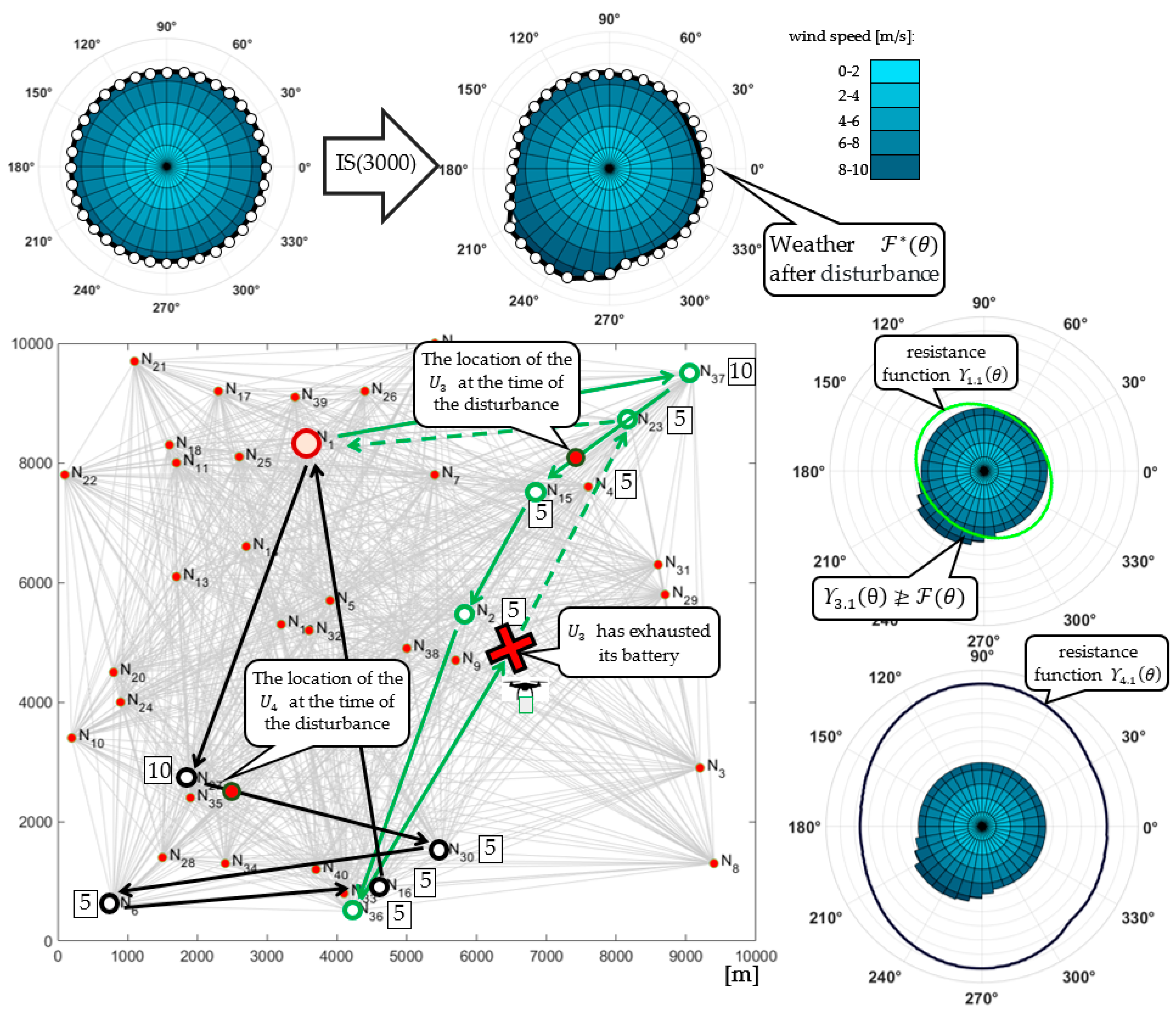
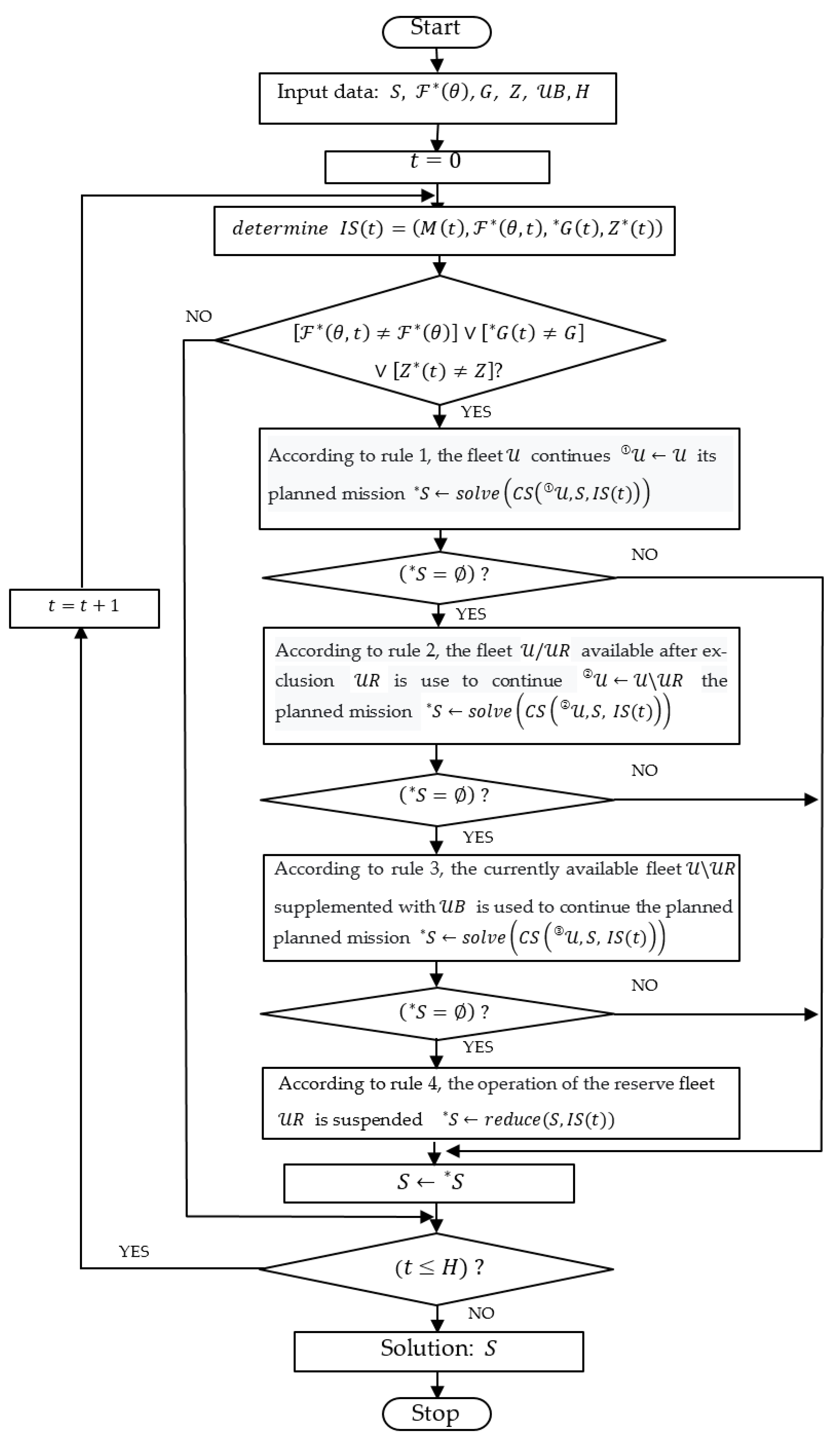
• If the adopted mission plan S is not resistant to disturbance $IS\left(t^{*}\right)$ $\left({\exists }_{k\in \left\{1,\dots ,K\right\},l\in \left\{1,\dots ,L\right\}}{{\rm Y}}_{k,l}\left(\theta \right)\ngeqq ℱ\left(\theta \right)\right),$ then it should be checked whether it is possible to adapt (re-plan), adjusting it to new conditions. That is, decide whether all UAVs in the air continue their current missions or make their appropriate corrections.
• If there are UAVs (the set $\mathcal{U}R$) that cannot continue to fly due to disturbance $IS\left(t^{*}\right),$ then they should be returned to the base after it is ensured that airborne UAVs ($\mathrm{the} \mathrm{set} \mathcal{U}\backslash \mathcal{U}R$) can take over their tasks.
• If the tasks of the UAVs returning to the base (the set $\mathcal{U}R)$ cannot be taken over by UAVs still performing their missions, then it should be checked whether the reserve UAVs available at the base (the set $\mathcal{U}B$) can take over their responsibilities. This means the UAVs in the air continue their existing missions, while the reserve UAVs take over the liabilities of the UAVs returned to the base.
• If the reserve UAVs (the set $\mathcal{U}B$) are unable to take over the responsibilities of those returned to the base (the set $\mathcal{U}R$), then their activity should be suspended until the disturbance is resolved.

The above rules have been used in the reactive mission planning method $S$ shown in Figure 4. The idea behind this method is as follows. During the implementation of mission $S$, there is continuous monitoring of the state of the $IS\left(t\right)$ (for $t\in \left\{0\dots H\right\}$). If at the state $IS\left(t\right),$ the following condition holds $\left[{ℱ}^{*}\left(\theta ,t^{*}\right)\ne {ℱ}^{*}\left(\theta \right)\right]\vee \left[{}_{ }{}^{*}G\left(t^{*}\right)\ne G\right]\vee \left[Z^{*}\left(t^{*}\right)\ne Z\right]$ (e.g., there is a change in the weather forecast or in the structure of the distribution network as well as in the size of the requests) and mission $S$ is under threat (i.e., at least one of the UAVs will not return to base due to low battery), then an attempt is made to replan it. Such reaction is performed by the function solve, the purpose of which is to designate a mission ${}_{ }{}^{*}S$ adapted to the new conditions determined by the disturbance $IS\left(t\right)$.

In practice, it comes down to solving the relevant constraints satisfaction problem $CS\left({}_{ }{}^O\mathcal{U},S, IS\left(t\right)\right)$ (where:${}_{ }{}^O\mathcal{U}$—defines the fleet designated by condition action rules 1–4. The relevant constraints distribution process follows the sequence where at first, an attempt is made to designate mission ${}_{ }{}^{*}S$ for the fleet ${}_{ }{}^{➀}\mathcal{U}=\mathcal{U}$ (according to rule 1). In the event of failure, an attempt is made to designate it for the fleet ${}_{ }{}^{➁}\mathcal{U}=\mathcal{U}\backslash \mathcal{U}R$ (according to rule 2 and then for the fleet ${}_{ }{}^{➂}\mathcal{U}=\left(\mathcal{U}\backslash \mathcal{U}R\right)\cup \mathcal{U}B$ (according to rule 3). If an admissible solution ${}_{ }{}^{*}S$ still does not exist, then the currently used mission plan should be modified (due to the $reduce$ function) in such a way that it removes the sub-missions, which are not resistant to disturbance $IS\left(t\right)$ (according to rule 4).

It should be noted that the designation of mission ${}_{ }{}^{*}S$ is associated with the designation of routings ${}_{ }{}^l\Pi$, schedules ${}_{ }{}^{l}Y$, and delivery sequences ${}_{ }{}^{l}C$ throughout the remaining time horizon $\left\{t,\dots ,H\right\}$.

Due to the disturbance $IS\left(t^{*}\right)$ occurrence, the proposed reactive planning algorithm (implemented in the IBM ILOG environment) generates the end-to-end paths that modify previously planned routes, restoring the ability to implement the designated mission delivery plan.

2.3.2. Declarative Modelling

The mathematical formulation of the constraint satisfaction problem $CS\left({}_{ }{}^O\mathcal{U},S, IS\left(t\right)\right)$ aimed at reactive planning of the mission employs the following parameters, variables, sets, and constraints.

Parameters:

${}_{ }{}^{l}G$	the graph of a distribution network: ${}_{ }{}^{l}G=\left(N, E\right)$ for sub-mission ${}_{ }{}^{l}S$, where: $N=\left\{N_1,\dots ,N_{\lambda },\dots ,N_n\right\}$ is the set of nodes, $E=\left\{\left(N_i,N_j\right)| i, j \in \left\{1,\dots ,n\right\}, i \ne j\right\}$ is the set of edges
$z_{\lambda }$	the demand at node $N_{\lambda }$, $z_1=0$
$d_{\beta ,\lambda }$	the travel distance between nodes $N_{\beta }$,$N_{\lambda }$
$t_{\beta ,\lambda }$	the travel time between nodes $N_{\beta }$,$N_{\lambda }$
$w$	the time spent on take-off and landing of a UAV
$ts$	the time interval at which UAVs can take off from the base
${}_{ }{}^l\mathcal{U}$	the subset of UAVs ${}_{ }{}^l\mathcal{U}\subseteq \mathcal{U}=\left\{U_1,\dots ,U_k,\dots , U_K\right\}$ carrying out the sub-mission ${}_{ }{}^{l}S$, where: $U_k$ is the k-th UAV
$K$	the size of the fleet of UAVs
$IS\left(t\right)$	the state of UAVs mission at the time $t$: $IS\left(t\right)=\left(M\left(t\right), {ℱ}^{*}\left(\theta ,t\right),{}_{ }{}^{*}G\left(t\right),Z^{*}\left(t\right)\right)$
${{\rm Y}}_{k,l}\left(\theta \right)$	$U_k$ resistance to changes in weather conditions during the execution of the plan of mission ${}_{ }{}^{l}S$
$Q$	the maximum loading capacity of a UAV
$C_D$	the aerodynamic drag coefficient of a UAV
$A$	the front-facing area of a UAV
$ep$	the empty weight of a UAV
$D$	an air density
$g$	the gravitational acceleration
$b$	the width of a UAV
$CAP$	the maximum energy capacity of a UAV
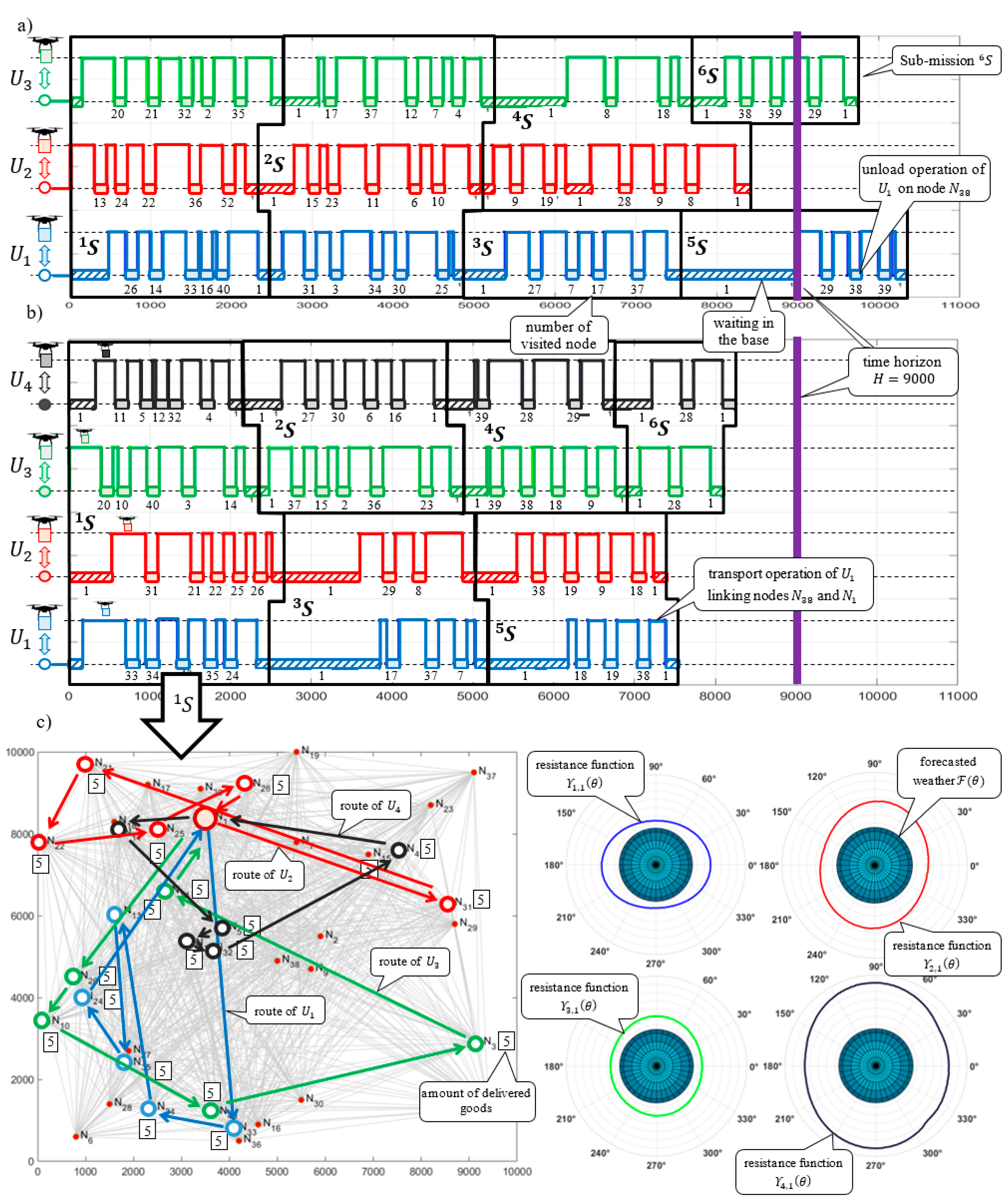
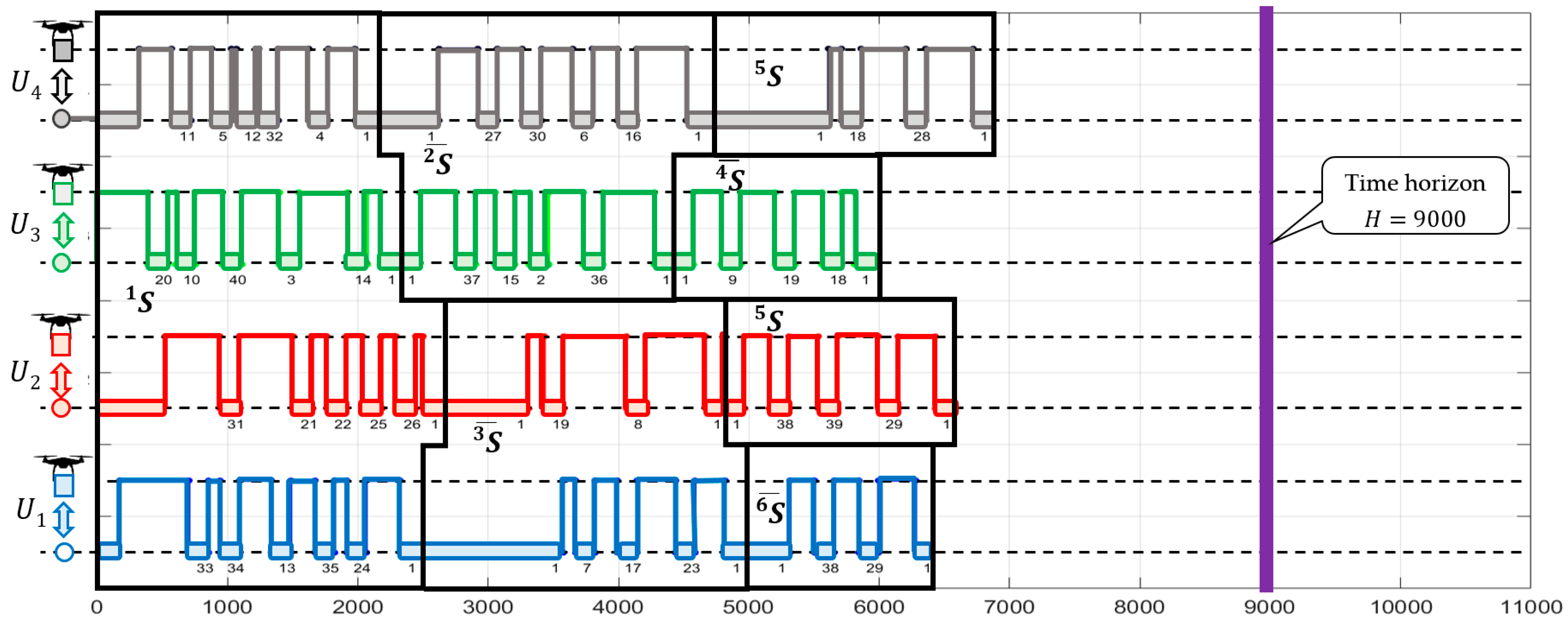
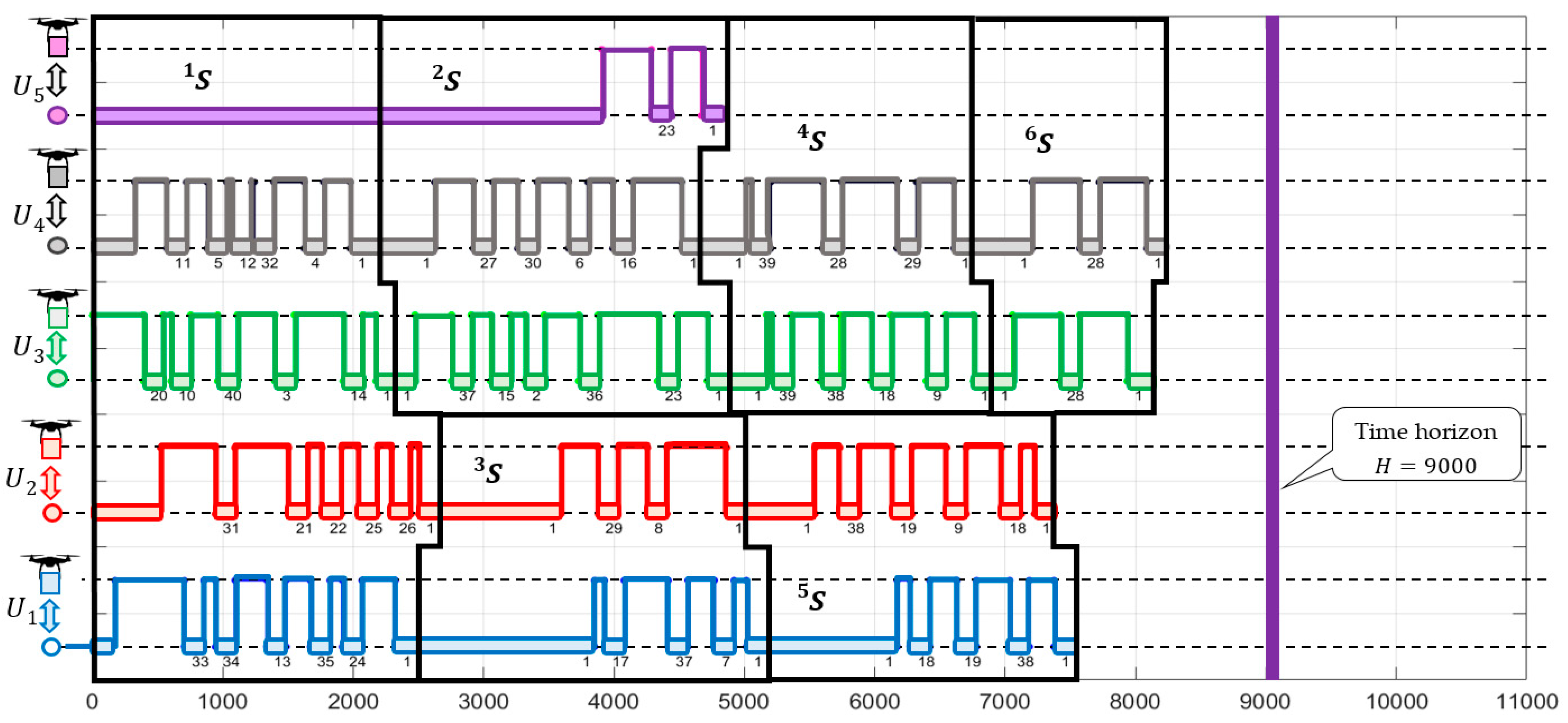
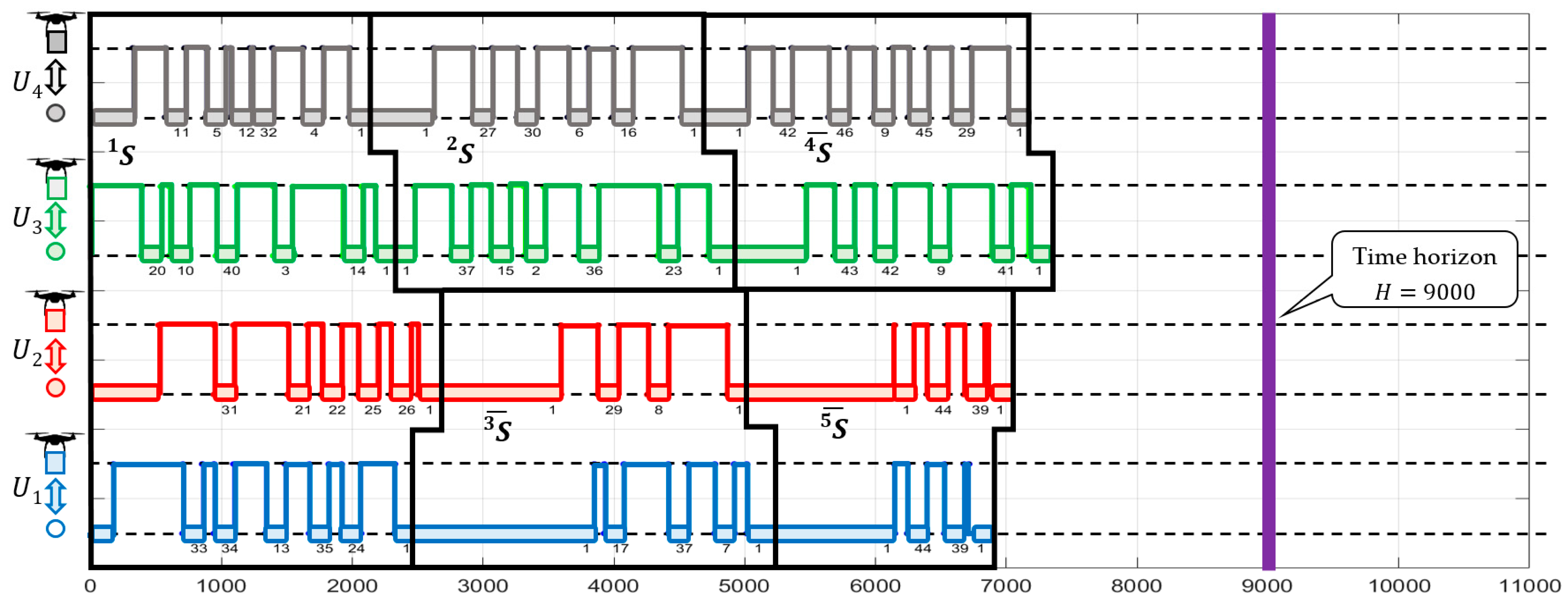
$H$	the time horizon (see Figure 2b—$H=9000$)
$ℱ{\left(\theta \right)}^{ }$	the function values of which determine the maximum of forecasted wind speed for given direction $\theta$
$v{a}_{\beta ,\lambda }^{ }$	an airspeed of a UAV traveling between nodes $N_{\beta }$,$N_{\lambda }$
${\phi }_{\beta ,\lambda }$	the heading angle, angle of the airspeed vector when the UAV travels between nodes $N_{\beta }$,$N_{\lambda }$
$v{g}_{\beta ,\lambda }^{ }$	the ground speed of a UAV traveling between nodes $N_{\beta }$,$N_{\lambda }$
${\vartheta }_{\beta ,\lambda }$	the course angle, angle of the ground speed vector when the UAV travels between nodes $N_{\beta }$,$N_{\lambda }$
${}_{ }{}^{l}S{}_{ }$	the plan of sub-mission: ${}_{ }{}^{l}S=\left({}_{ }{}^l\mathcal{U},{}_{ }{}^l\Pi ,{}_{ }{}^{l}Y,{}_{ }{}^{l}C\right)$ when there is no disturbance: ${}_{ }{}^{l}Y$: is a sequence of moments ${}_{ }{}^{l}y{}_{\lambda }^k$ (i.e., the fleet ${}_{ }{}^l\mathcal{U}$ schedule): ${}_{ }{}^{l}Y=\left({}_{ }{}^{l}y{}_1^1,\dots ,{}_{ }{}^{l}y{}_1^K,\dots ,{}_{ }{}^{l}y{}_n^1,\dots ,{}_{ }{}^{l}y{}_n^K\right)$, ${}_{ }{}^{l}y{}_{\lambda }^k$ is the time at which $U_k$ arrives at node $N_{\lambda }$, ${}_{ }{}^l\Pi$: the set of UAV routes ${}_{ }{}^l\pi {}_k^{ }$: ${}_{ }{}^l\pi {}_k=\left(N_{k_1},\dots ,N_{k_i},N_{k_{i+1}},\dots ,N_{k_{\mu }}\right)$ ${}_{ }{}^{l}C$: is a sequence of weights of delivered goods ${}_{ }{}^{l}c{}_{\lambda }^k$: $C^k=\left({}_{ }{}^{ }c{}_1^k,\dots , {}_{ }{}^{ }c{}_{\lambda }^k,\dots ,{}_{ }{}^{ }c{}_n^k\right)$, ${}_{ }{}^{l}c{}_{\lambda }^k$ is the weight of goods delivered to node $N_{\lambda }$ by $U_k$
$S$	the flight mission plan $S=\left({}_{ }{}^{1}S,\dots ,{}_{ }{}^{l}S,\dots ,{}_{ }{}^{L}S\right)$, where: $L$ denotes the number of sub-missions.

Decision Variables:

$\overline{{}_{ }{}^{l}x{}_{\beta ,\lambda }^k}$	the binary variable used to indicate if $U_k$ travels between nodes $N_{\beta }$,$N_{\lambda }$, after the disturbance $IS\left(t^{*}\right)$ occurrence (during sub-mission ${}_{ }{}^{l}S$)
$\overline{{}_{ }{}^{l}x{}_{\beta ,\lambda }^k}=\{\begin{array}{cc}1& \mathrm{if} U_k{ \mathrm{travels} \mathrm{between} \mathrm{nodes} N}_{\mathsf{\beta }}{, N}_{\mathsf{\lambda }}\\ 0& \mathrm{otherwise}\end{array}$
$\overline{{}_{ }{}^{l}y{}_{\lambda }^k}$	the time at which $U_k$ arrives at node $N_{\lambda }$, after the disturbance $IS\left(t^{*}\right)$ occurrence (during sub-mission ${}_{ }{}^{l}S$)
$\overline{{}_{ }{}^{l}c{}_{\lambda }^k}$	the weight of freight delivered to node $N_{\lambda }$ by $U_k$, after the disturbance $IS\left(t^{*}\right)$ occurrence (during sub-mission ${}_{ }{}^{l}S$)
$\overline{{}_{ }{}^{l}f{}_{\beta ,\lambda }^k}$	the weight of freight carried between nodes $N_{\beta }$,$N_{\lambda }$ by $U_k$, after the disturbance $IS\left(t^{*}\right)$ occurrence (during sub-mission ${}_{ }{}^{l}S$)
$\overline{{}_{ }{}^{l}P{}_{\beta ,\lambda }^k}$	the energy per unit of time consumed by $U_k$ during the flight between nodes $N_{\beta }$,$N_{\lambda }$ (after the disturbance $IS\left(t^{*}\right)$ occurrence)
$\overline{{}_{ }{}^{l}ba{t}^k}$	the total energy consumed by $U_k$, after the disturbance $IS\left(t^{*}\right)$ occurrence (during sub-mission ${}_{ }{}^{l}S$)
$\overline{{}_{ }{}^{l}s{}^k}$	the take-off time of $U_k$, after the disturbance $IS\left(t^{*}\right)$ occurrence (during sub-mission ${}_{ }{}^{l}S$)
$\overline{{}_{ }{}^{l}c{p}_{\lambda }}$	the total weight of freight delivered to node $N_{\lambda }$, after the disturbance $IS\left(t^{*}\right)$ occurrence (during sub-mission ${}_{ }{}^{l}S$)
$\overline{{}_{ }{}^l\pi {}_k^{ }}$	the route of $U_k$ after the disturbance $IS\left(t^{*}\right)$ occurrence (during sub-mission ${}_{ }{}^{l}S$), $\overline{{}_{ }{}^l\pi {}_k}=(N_{k_1},\dots ,N_{k_i},N_{k_{i+1}},\dots ,N_{k_{\mu }}$, $k_i\in \left\{1,\dots ,n\right\}$, $\left(N_{k_i},N_{k_{i+1}}\right)\in E$.

Sets:

$\overline{{}_{ }{}^{l}Y}$	is a sequence of moments $\overline{{}_{ }{}^{l}y{}_{\lambda }^k}$, schedule of the fleet ${}_{ }{}^l\mathcal{U}$ after the disturbance $IS\left(t^{*}\right)$ occurrence
$\overline{{}_{ }{}^{l}C}$	$\mathrm{is} \mathrm{a} \mathrm{sequence} \mathrm{of} \mathrm{weights} \mathrm{of} \mathrm{delivered} \mathrm{goods} \overline{{}_{ }{}^{l}c{}_{\lambda }^k}$
$\overline{{}_{ }{}^l\Pi }$	$\mathrm{the} \mathrm{set} \mathrm{of} \mathrm{UAV} \mathrm{routes} \overline{{}_{ }{}^l\pi {}_k^{ }}$
${\overline{{}_{ }{}^{l}S}}_{ }$	$\mathrm{the} \mathrm{plan} \mathrm{of} \mathrm{sub}\text{-}\mathrm{mission} \mathrm{after} \mathrm{the} \mathrm{disturbance} IS\left(t^{*}\right)$$\mathrm{occurrence}: \overline{{}_{ }{}^{l}S}=\left({}_{ }{}^l\mathcal{U},\overline{{}_{ }{}^l\Pi },\overline{{}_{ }{}^{l}Y},\overline{{}_{ }{}^{l}C}\right)$
${}_{ }{}^{*}S$	$\mathrm{the} \mathrm{re}\text{-}\mathrm{route} \mathrm{plan} \mathrm{of} \mathrm{the} \mathrm{mission}: {}_{ }{}^{*}S=\left({\overline{{}_{ }{}^{1}S}}_{ },\dots ,{\overline{{}_{ }{}^{l}S}}_{ },\dots ,{\overline{{}_{ }{}^{L}S}}_{ }\right).$

Constraints limiting: routes, delivery of freight, and energy consumption

• Routes. Relationships between the variables describing UAV take-off times/mission start times and task order:

$$\overline{{}_{ }{}^{l}s{}^k}\ge 0; k=1,\dots ,K;=1,\dots ,L,$$

(2)

$$\left({}_{ }{}^{l}s{}^k\le t^{*}\right)\Rightarrow \left(\overline{{}_{ }{}^{l}s{}^k}={}_{ }{}^{l}s{}^k\right); k=1,\dots ,K; l=1,\dots ,L,$$

(3)

$$\left(\left|\overline{{}_{ }{}^{l}s{}^k}-\overline{{}_{ }{}^{l}s{}^q}\right|\ge ts\right) ;k,q=1\dots K; k\ne q; l=1,\dots ,L,$$

(4)

$$\left( {}_{ }{}^{l}y{}_j^k\le t^{*}\right)\Rightarrow \left(\overline{{}_{ }{}^{l}x{}_{i,j}^k}={}_{ }{}^{l}x{}_{i,j}^k\right); j=1\dots n; i=2,\dots ,n; k=1,\dots ,K; l=1\dots L,$$

(5)

$$\left( {}_{ }{}^{l}y{}_j^k\le t^{*}\right)\Rightarrow \left(\overline{{}_{ }{}^{l}y{}_j^k}={}_{ }{}^{l}y{}_j^k\right); j=1,\dots ,n; i=2,\dots ,n; k=1,\dots ,K; l=1,\dots ,L,$$

(6)

$${{\displaystyle \sum }}_{j=1}^n\overline{{}_{ }{}^{l}x{}_{i,j}^k}=1 ; k=1,\dots ,K; l=1,\dots ,L,$$

(7)

$$\left(\overline{{}_{ }{}^{l}x{}_{1,j}^k}=1\right)\Rightarrow \left(\overline{{}_{ }{}^{l}y{}_j^k}=\overline{{}_{ }{}^{l}s{}^k}+t_{1,j}\right) ; j=1,\dots ,n; k=1,\dots ,K,$$

(8)

$$\begin{gathered} \left(\overline{{}_{ }{}^{l}y{}_i^k}\ne 0 \wedge \overline{{}_{ }{}^{l}y{}_i^q}\ne 0 \right)\Rightarrow \left(\left|\overline{{}_{ }{}^{l}y{}_i^k}-\overline{{}_{ }{}^{l}y{}_i^q}\right|\ge w\right) ;i=1,\dots ,n; k,q=1,\dots ,K; \\ k\ne q, \end{gathered}$$

(9)

$$\left(\overline{{}_{ }{}^{l}x{}_{i,j}^k}=1\right)\Rightarrow \left(\overline{{}_{ }{}^{l}y{}_j^k}=\overline{{}_{ }{}^{l}y{}_i^k}+t_{i,j}+w\right); j=1,\dots ,n; i=2,\dots ,n; k=1,\dots ,K ,$$

(10)

$$\overline{{}_{ }{}^{l}y{}_i^k}\ge 0; i=1,\dots ,n; k=1,\dots ,K,$$

(11)

$${{\displaystyle \sum }}_{j=1}^n\overline{{}_{ }{}^{l}x{}_{i,j}^k}={{\displaystyle \sum }}_{j=1}^n\overline{{}_{ }{}^{l}x{}_{j,i}^k}; i=1,\dots ,n; k=1,\dots ,K,$$

(12)

$$\overline{{}_{ }{}^{l}y{}_i^k}\le H\times {{\displaystyle \sum }}_{j=1}^n\overline{{}_{ }{}^{l}x{}_{i,j}^k}, i=1,\dots ,n; k=1,\dots ,K,$$

(13)

$$\overline{{}_{ }{}^{l}x{}_{i,i}^k}=0; i=1,\dots ,n; k=1,\dots ,K.$$

(14)

2.

Delivery of freight. Relationships between variables describing already delivered and requested amount of freight:

$$\left( \overline{{}_{ }{}^{l}y{}_j^k}\le t^{*}\right)\Rightarrow \left(\overline{{}_{ }{}^{l}c{}_j^k}={}_{ }{}^{l}c{}_j^k\right);=1,\dots ,n; i=2,\dots ,n; k=1,\dots ,K; l=1,\dots ,L,$$

(15)

$$\overline{{}_{ }{}^{l}c{}_i^k}\ge 0; i=1,\dots ,n; k=1,\dots ,K;l=1,\dots ,L,$$

(16)

$$\overline{{}_{ }{}^{l}c{}_i^k}\le Q\times {{\displaystyle \sum }}_{j=1}^n{x}_{i,j}^k; i=1,\dots ,n; k=1,\dots ,K; l=1,\dots ,L,$$

(17)

$${{\displaystyle \sum }}_{i=1}^n\overline{{}_{ }{}^{l}c{}_i^k}\le Q; k=1,\dots ,K;l=1,\dots ,L,$$

(18)

$$\left(\overline{{}_{ }{}^{l}x{}_{i,j}^k}=1 \right)\Rightarrow \left(\overline{{}_{ }{}^{l}c{}_i^k}\ge 1\right); k=1,\dots ,K; i=1,\dots ,n; j=2,\dots ,n,$$

(19)

$${{\displaystyle \sum }}_{l=1}^L{{\displaystyle \sum }}_{k=1}^K\overline{{}_{ }{}^{l}c{}_i^k}=z_i; i=1,\dots ,n ,$$

(20)

$${{\displaystyle \sum }}_{i=1}^n\overline{{}_{ }{}^{l}c{}_i^k}=\overline{{}_{ }{}^{l}c{s}^k}; k=1,\dots ,K;=1,\dots ,L,$$

(21)

$$\left(\overline{{}_{ }{}^{l}x{}_{i,j}^k}=1\right)\Rightarrow \left(\overline{{}_{ }{}^{l}f{c}_j^k}=\overline{{}_{ }{}^{l}c{s}^k}\right) ;j=1\dots n; k=1\dots K; l=1,\dots ,L,$$

(22)

$$\left(\overline{{}_{ }{}^{l}x{}_{i,j}^k}=1\right)\Rightarrow \left(\overline{{}_{ }{}^{l}f{c}_j^k}=\overline{f{c}_i^k}-\overline{{}_{ }{}^{l}c{}_i^k}\right) ;i,j=1,\dots ,n; k=1\dots K; l=1,\dots ,L,$$

(23)

$$\left(\overline{{}_{ }{}^{l}x{}_{i,j}^k}=1\right)\Rightarrow \left(\overline{{}_{ }{}^{l}f{}_{1,j}^k}=\overline{{}_{ }{}^{l}c{s}^k}\right) ;j=1,\dots ,n; k=1\dots K; l=1,\dots ,L,$$

(24)

$$\left(\overline{{}_{ }{}^{l}x{}_{i,j}^k}=1\right)\Rightarrow \left(\overline{{}_{ }{}^{l}f{}_{i,j}^k}=\overline{{}_{ }{}^{l}f{c}_j^k}\right) ; i,j=1,\dots ,n; k=1,\dots ,K; l=1,\dots ,L,$$

(25)

3.

Energy consumption. In order to ensure the waterproofness of the ${}_{ }{}^{l}S$ sub-mission (i.e., its robustness to weather condition changes $Z\left(\theta \right)$), it is necessary that the amount of energy required to complete the task carried out by a UAV does not exceed the capacity of its battery.

$${{\rm Y}}_{k,l}\left(\theta \right)\ge ℱ\left(\theta \right); \forall \theta \in \left[0^{\circ },{360}^{\circ }\right),$$

(26)

$${{\rm Y}}_{k,l}\left(\theta \right)=\max {\Gamma }_{k,l}\left(\theta \right),$$

(27)

$${\Gamma }_{k,l}\left(\theta \right)=\left\{vw | vw\in R_{+}^0\wedge \forall { }_{k\in \left\{1\dots K\right\}}\overline{{}_{ }{}^{l}ba{t}^k}\left(\theta ,vw\right)\le CAP\right\},$$

(28)

$$\overline{{}_{ }{}^{l}ba{t}^k}\left(\theta ,vw\right)={{\displaystyle \sum }}_{i=1}^n{{\displaystyle \sum }}_{j=1}^n\overline{{}_{ }{}^{l}x{}_{i,j}^k}\times t_{i,j}\times {}_{ }{}^{l}P{}_{i,j}^k\left(\theta ,vw\right),$$

(29)

$$\overline{{}_{ }{}^{l}ba{t}^k}\left(\theta ,vw\right)={{\displaystyle \sum }}_{i=1}^n{{\displaystyle \sum }}_{j=1}^n\overline{{}_{ }{}^{l}x{}_{i,j}^k}\times t_{i,j}\times {}_{ }{}^{l}P{}_{i,j}^k\left(\theta ,vw\right),$$

(30)

where: ${}_{ }{}^{l}v{a}_{i,j}^{ }\left(\theta ,vw\right)$ and $t_{i,j}$ depend on the assumed goods delivering strategy.

If the ground speed $v{g}_{i,j}^{ }$ is constant, then an airspeed ${}_{ }{}^{l}v{a}_{i,j}^{ }$ is calculated from:

$$\begin{gathered} {}_{ }{}^{l}v{a}_{i,j}^{ }\left(\theta ,vw\right)= \\ \sqrt{{\left(v{g}_{i,j}^{ }\times cos{\vartheta }_{i,j}-vw\times cos{\theta }_{ }\right)}^2+{\left(v{g}_{i,j}^{ }\times sin{\vartheta }_{i,j}-vw\times sin{\theta }_{ }\right)}^2}, \end{gathered}$$

(31)

$$t_{i,j}=\frac{d_{i,j}}{v{g}_{i,j}^{ }}.$$

(32)

The constraints (1)–(13) describe the relationship between UAV routes (represented by the variables $\overline{{}_{ }{}^{l}x{}_{i,j}^k}$) and the delivery schedule (variables $\overline{{}_{ }{}^{l}y{}_i^k}$ and $\overline{{}_{ }{}^{l}s{}^k}$). They provide, among others, that it is not possible for several UAVs to take off from the base at the same time (3), that there is no possibility of simultaneous occupation of a common recipient by several UAVs (8), that service of delivery points must be in accordance with the adopted route (7), (9), and so on. Constraints (14)–(24), in turn, link UAV routes ($\overline{{}_{ }{}^{l}x{}_{i,j}^k}$) to the number of goods delivered (variables $\overline{{}_{ }{}^{l}c{}_i^k}$). They also ensure that the UAVs are not overloaded (17), the correct amount of goods is delivered (19), and determine the weight ($\overline{{}_{ }{}^{l}f{}_{\beta ,\lambda }^k}$) of the goods carried on each section of the taken route (21)–(24). Constraints (25)–(31) determine the values of the determined resistance functions ${{\rm Y}}_{k,l}\left(\theta \right)$ for UAVs (26)–(31) and ensure that its values exceed the value set on the function $ℱ\left(\theta \right)$ (determining forecasted weather conditions).

Since the re-planning of the mission delivery plan S is the result of the disturbance $IS\left(t^{*}\right)$, hence the new set of sub-missions ${\overline{{}_{ }{}^{1}S}}_{ },\dots ,{\overline{{}_{ }{}^{l}S}}_{ },\dots ,{\overline{{}_{ }{}^{L}S}}_{ }$ guaranteeing timely delivery are determined by solving the following Constraint Satisfaction (CS) Problem (32):

$$CS\left({}_{ }{}^O\mathcal{U},S, IS\left(t^{*}\right)\right)=\left(\left(\mathcal{V},\mathcal{D}\right),\mathcal{C}\left({}^O\mathcal{U},S, IS\left(t^{*}\right)\right)\right),$$

(33)

where:

$\widehat{\mathcal{V}}=\left\{\overline{{}_{ }{}^l\Pi },\overline{{}_{ }{}^{l}Y},\overline{{}_{ }{}^{l}C}|l=1\dots L\right\}$—the set of decision variables: $\overline{{}_{ }{}^l\Pi }$—the set of routes determining the schedule $\overline{{}_{ }{}^{l}Y}$, $\overline{{}_{ }{}^{l}Y}$—schedule of the fleet ${}_{ }{}^O\mathcal{U}$ guarantees timely service of delivery points in the case of disturbance $IS\left(t^{*}\right)$, and $\overline{{}_{ }{}^{l}C}$—sequence of weights of delivered goods by the fleet ${}_{ }{}^O\mathcal{U}$.

$\mathcal{D}$—the finite set of decision variable domains: $\overline{{}_{ }{}^{l}x{}_{i,j}^k}\in \left\{0,1\right\}$, $\overline{{}_{ }{}^{l}y{}_{\lambda }^k}\in \mathbb{N}$, $\overline{{}_{ }{}^{l}c{}_i^k}\in \mathbb{N}$

$\widehat{\mathcal{C}}$—the set of constraints that take into account the set of routes $\overline{{}_{ }{}^l\Pi }$, schedules $\overline{{}_{ }{}^{l}Y,}$ and the disturbance $IS\left(t^{*}\right)$, while determining the relationships linking the operations executed by UAVs (1)–(31).

To solve $CS$ (32), the values of the decision variables from the adopted set of domains for which the given constraints are satisfied must be determined.

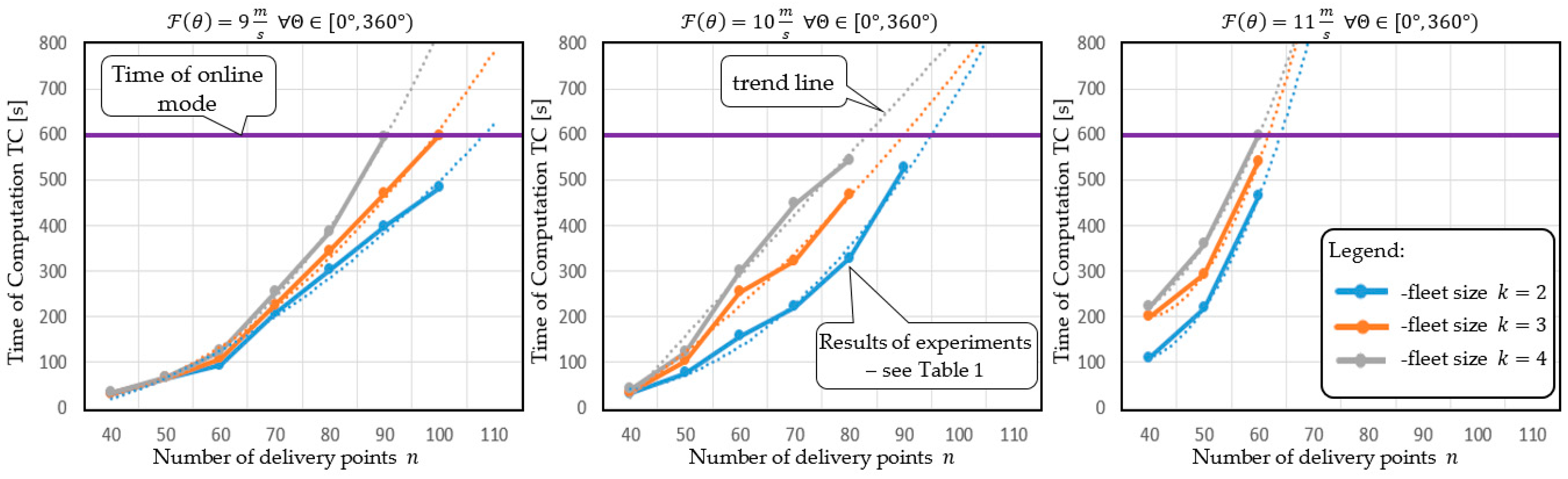
3. Results-Computational Experiments

We consider the network from Figure 1, in which the four UAVs $\mathcal{U}=\left\{U_1,U_2,U_3,U_4\right\}$ service delivery points $N_2–N_{40}$ according to the proactive plan from Figure 2b. The structure of the implementation of subsequent sub-missions ${}_{ }{}^{1}S,{}_{ }{}^{2}S,\dots ,{}_{ }{}^{6}S$ of the adopted mission plan $S$ is presented in Figure 3.

Let us consider a situation related to the appearance of a disturbance IS(3000), specified in Section 2.2, where at the time $t^{*}=3000 \mathrm{s}$, during the execution of sub-mission ${}_{ }{}^{2}S$, the wind speed increased to $vw=11\frac{m}{s}$ with the same wind intensity and direction $\theta =210°–230°$. With such a change in weather conditions, the implementation of the adopted plan turns out to be impossible.

It becomes necessary to re-plan the implemented mission, including the introduction of sub-missions $\overline{{}_{ }{}^{2}S},\overline{{}_{ }{}^{3}S}$,$\overline{{}_{ }{}^{4}S}$,$\overline{{}_{ }{}^{5}S},\overline{{}_{ }{}^{6}S}$ to correct its course. For this purpose, an algorithm from Figure 4 modeled in $CS$ (32) formalism has been used. Its implementation in the constraint programming environment IBM ILOG (Windows 10, Intel Core i7-M4800MQ 2.7 GHz, 32 GB RAM) has shown that the solution time for problems of the size considered does not exceed 25 s.

Figure 5 shows the mission ${}_{ }{}^{*}S$ schedule adapted to the weather conditions determined by the disturbance $IS\left(3000\right)$. Rule 2 was used in assigning mission ${}_{ }{}^{*}S$, i.e., if there are UAVs (the set $\mathcal{U}R$) that cannot continue to fly due to disturbance $IS\left(t^{*}\right),$ then they should be returned to the base, and after it is ensured that airborne UAVs ($\mathrm{the} \mathrm{set} \mathcal{U}\backslash \mathcal{U}R$) can take over their tasks. Accordingly, as a result of the $IS \left(3000\right)$ disturbance, the decision to turn $U_3$ back to the base was made (see sub-mission $\overline{{}_{ }{}^{2}S}$) because there was a risk of premature battery depletion. At the same time, $U_4$ continued its mission unchanged. This decision forced the necessity to reschedule subsequent sub-missions $\overline{{}_{ }{}^{3}S}$,$\overline{{}_{ }{}^{4}S}$,$\overline{{}_{ }{}^{5}S},\overline{{}_{ }{}^{6}S}$—Figure 6, which allowed for the designation of a new alternative plan ${}_{ }{}^{*}S,$ taking into account the conditions of the disturbance $IS\left(3000\right)$—see the path marked in blue in the graph from Figure 6.

Figure 7 shows an alternative variant of the disturbance response based on rule 3, i.e., if the tasks of a UAV returning to the base (the set $\mathcal{U}R)$ cannot be taken over by UAVs still performing their missions, then it should be checked whether the reserve UAVs available in the base (the set $\mathcal{U}B$) can take over their responsibilities. In the proposed solution, similar to the previous one, the decision was made to return $U_3$ to the base (see sub-mission $\overline{{}_{ }{}^{2}S}$). The functions of $U_3$ (execution of deliveries to the point $N_{23}$) were taken over by the reserve $U_5$. Such a solution does not interfere with the implementation of the remaining UAVs, which allows them to return and continue (beginning from sub-mission $\overline{{}_{ }{}^{4}S}$) the originally established reactive plan: $\overline{{}_{ }{}^{4}S}={}_{ }{}^{4}S$,$\overline{{}_{ }{}^{5}S}={}_{ }{}^{5}S,\overline{{}_{ }{}^{6}S}={}_{ }{}^{6}S$—see the path marked in orange in the graph from Figure 6.

As part of the conducted experiments, a case related to the occurrence of a disturbance caused by a change in the structure of the network $G^{*}$ (including elements of the set of served delivery points) was also considered. The case under consideration concerns the situation (i.e., the disturbance IS (4800)) in which at the time $t^{*}=4800 \mathrm{s}$, during the execution of sub-mission ${}_{ }{}^{3}S$, four delivery points $N_{18}$, $N_{28}$, $N_{38}$, $N_{19}$ give up previously ordered deliveries and six new ones $N_{41}$–$N_{46}$ submit their orders.

Figure 8 shows the current structure of the distribution network. This disturbance makes the adopted mission plans (in particular ${}_{ }{}^{3}S$, ${}_{ }{}^{4}S$, ${}_{ }{}^{5}S$) insufficient–it becomes necessary to redesign them. Consequently, due to the reactive planning algorithm from Figure 4, rule 1 was used to design a new mission ${}_{ }{}^{*}S$ plan, i.e., if the adopted mission plan S is not admissible to disturbance $IS\left(4800\right),$ then it should be checked whether it is possible to adapt (re-plan), adjusting it to new conditions.

Figure 9 shows the modification (calculated in less than 16 s) of the mission plan ${}_{ }{}^{*}S$ caused by the disturbance IS (4800) and implying the designation of new sub-missions $\overline{{}_{ }{}^{3}S}$, $\overline{{}_{ }{}^{4}S}$, $\overline{{}_{ }{}^{5}S}$ (see scenario marked in Figure 6 with a purple line). Despite the newly added delivery points, all pre-scheduled deliveries were completed within the given time horizon.

The presented example shows that the determination of reactive mission plans can be done online, i.e., in a time not exceeding 30 s.

To assess the scalability of the proposed approach in terms of the possibility of its use in an online mode (i.e., to solve the problem in <600 s) in decision support systems, a series of quantitative experiments have been carried out.

Table 1. Results of the experiments conducted.

		Number of Sub-Missions	$ℱ\left(\theta \right)=9\frac{\mathit{m}}{\mathit{s}}$ $\forall \Theta \in \left[0°,360°\right)$	Number of Sub-Missions	${ℱ}^{ }\left(\theta \right)=10\frac{\mathit{m}}{\mathit{s}}$ $\forall \Theta \in \left[0°,360°\right)$	Number of Sub-Missions	${ℱ}^{ }\left(\theta \right)=11\frac{\mathit{m}}{\mathit{s}}$ $\forall \Theta \in \left[0°,360°\right)$
${\displaystyle \mathit{n}}$	$\mathit{K}$		$\mathit{T}\mathit{C}$[s]		$\mathit{T}\mathit{C}$[s]		$\mathit{T}\mathit{C}$[s]
40	2	9	30.48	10	32.36	12	33.54
	3	8	32.39	9	34.79	10	40.60
	4	7	110.64	8	200.16	9	221.32
50	2	14	65.43	14	66.05	15	66.30
	3	12	76.51	13	102.72	15	122.54
	4	11	219.03	11	293.16	12	360.92
60	2	13	93.12	17	108.14	15	125.26
	3	15	157.14	16	253.91	17	300.65
	4	14	464.70	15	541.12	16	598.24
70	2	22	208.10	26	225.85	29	254.21
	3	21	221.42	22	322.41	24	448.48
	4	✖	t > 600	✖	t > 600	✖	t > 600
80	2	20	302.48	29	345.20	29	386.21
	3	23	328.01	24	469.14	25	544.57
	4	✖	t > 600	✖	t > 600	✖	t > 600
90	2	27	398.89	31	471.75	✖	t > 600
	3	21	526.24	✖	t > 600	✖	t > 600
	4	✖	t > 600	✖	t > 600	✖	t > 600
100	2	29	483.68	32	598.64	✖	t > 600
	3	✖	t > 600	✖	t > 600	✖	t > 600
	4	✖	t > 600	✖	t> 600	✖	t > 600
110	2	✖	t > 600	✖	t> 600	✖	t > 600
	3	✖	t > 600	✖	t > 600	✖	t > 600
	4	✖	t > 600	✖	t > 600	✖	t > 600

$n$—number of nodes (delivery points). $K$—size of the UAV fleet; $TC$—time of computation (s). ✖—no solution allowed in time t < 600 s.

contains the results of experiments that are conducted for the three functions of forecasted weather ${ℱ}^{ }\left(\theta \right)=9, 10, 11\frac{m}{s}$. The experiments are carried out for the network of $n$ randomly designated delivery points (on the area 10 km × 10 km) collection and a fleet consisting of $K$ UAVs with technical parameters as shown in Figure 1c. For each of the considered variants of the network, a proactive mission plan has been set out to guarantee the delivery in the time horizon $H=10000 \mathrm{s}$. It was assumed that at the moment $t^{*}=2000\mathrm{s}$, there is a change in the weather forecast (disturbance $IS\left(2000\right)$) that lasts until the end of the considered time horizon. The change in weather involves increasing the expected wind speed by 2 m/s and equals accordingly ${ℱ}^{*}\left(\theta \right)=11, 12, 13 \mathrm{m}/\mathrm{s}$. For each network, the UAV route planning is aimed at reactive performance of missions enabling deliveries in a given time horizon and in the expected weather conditions ${ℱ}^{*}\left(\theta \right)$. Results (i.e., the times $TC$ determining reactive mission plans design) are presented in Table 1, where symbol ✖ highlights those cases for which it was not possible to designate a mission plan in time $t<600 \mathrm{s}$.

4. Discussion

The NP-hard nature of the problem under consideration requires time-consuming calculations for most of the practical cases. The experiments allow for quantitative assessments of the scale of the distribution network for which the developed approach guarantees obtaining a reactive response in the online mode, i.e., in time t < 600 s. The conducted experiments (both qualitative and quantitative) show that for a distribution network of a size up to 90 delivery points and with a fleet of three UAVs (see Figure 10), the fleet mission plans can be effectively refined (in less than 600 s) and successfully carried out in changing weather conditions and after the occurrence of specific types of disturbances. The cases in which the computation time exceeds 600 s (see Table 1), mean that UAV cannot continue the planned mission (i.e., following rule 3, therefore it should return to base and suspend its activity until the disturbance is gone.)

The obtained results indicate that the adopted limitations force planning solutions consisting of many—in the considered experiments, not exceeding 35 sub-missions. The number of sub-missions needed to be accomplished increases as weather conditions $ℱ\left(\theta \right)$ worsen (imposing energy consumption increase) and the size of the fleet $\mathcal{U}$ decreases.

The obtained results show that the computer implementation of the developed algorithm (see Figure 4) within the constraint programming environment (e.g., IBM ILOG) will allow us to build a computing engine (solver) that enables the creation of an interactive decision support system. The set of questions that such a system could answer in the currently considered version includes:

• Emergency flight plan determination (beyond the allowable range defined by the weather change resistance functions ${{\rm Y}}_{k,l}\left(\theta \right))$.
• Determining the flight plan in the event of a sudden change of orders (change of the sequence $Z\left(t\right)$).
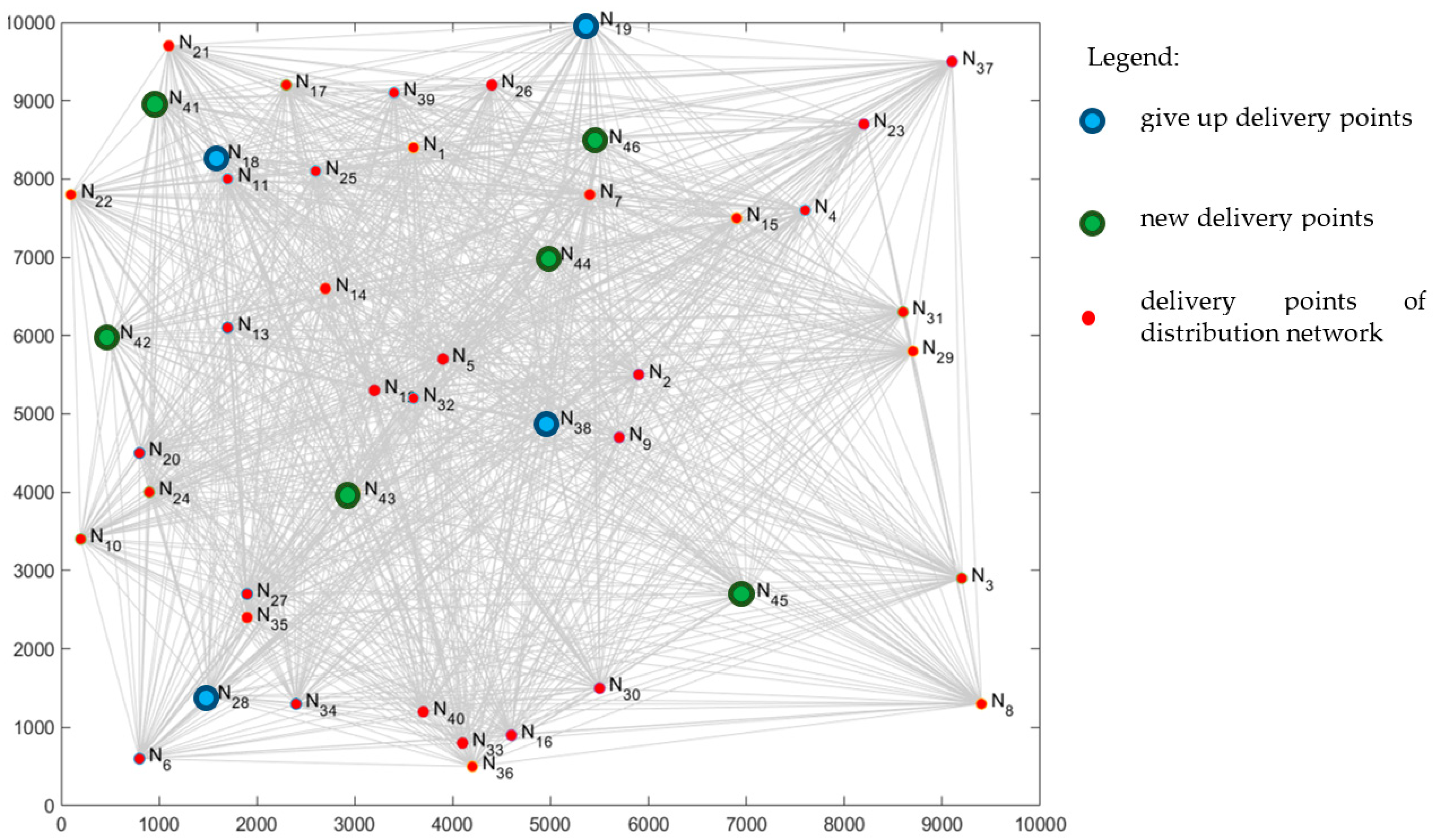
• Determining the flight plan in the event of a sudden change in the structure of the distribution network—i.e., the appearance of new or cancelation of previously placed orders (resulting in the change of network $G\left(t\right)$ structure).

The conducted experiments have demonstrated that the proposed set of rules (1–4 condition actions) enables the proposed system to work out a way (i.e., revised mission plan) that guarantees the achievement of a given mission objective (implementation of a given volume of supplies to a given number of consumers in a given time horizon $H$). It means that deliveries continue to all delivery points with no risk of discharging the UAV’s batteries. It is also worth emphasizing that our approach to the determining of reactive plans did not lead to exceeding the set delivery date (i.e., the time horizon $H$) in any of the analyzed cases.

The effectiveness of the developed method depends on the solvability of the developed problem $CS$ (32). In general, this problem is NP-hard, which means that for larger distribution networks, it is not possible to determine the mission plan in the online mode. The use of non-linear energy consumption constraints (25)–(31) is mainly responsible for this. The application of those constraints greatly increases the computational complexity of the problem, but it allows the system to accurately determine the range of weather conditions for which the designated mission is resistant (i.e., the battery is not discharged prematurely). The possibility of reducing computational complexity is seen in the development of constraints relaxation (25)–(31) to the form of linear equations. This will guarantee the same (or similar) level of energy consumption estimation. The construction of this type of constraint will be the subject of further research.

The presented method and the model behind it can also provide a basis for solving the more general problem of synthesis in which conditions (e.g., fleet size) are sought that guarantee the safe implementation of the expected deliveries after the appearance of a set of potential disturbances (changes in the weather, changes in orders, and changes in the network structure). The development of a method enabling the synthesis of these types of conditions constitutes a further direction for the conducted works.

5. Conclusions

In the future, UAVs may become a more frequent alternative to the use of traditional trucks in last-mile logistics and help improve the sustainability of urban freight transport. The delivery of goods in urban areas is subject to the occurrence of several disturbances. The proposed system’s ability to combine proactive and reactive planning can better solve real-life problems that arise in the field of urban freight transportation.

Our research contributes to the body of literature on planning and scheduling for UAV fleets. We propose a reactive routing method to solve the problem of UAV fleet mission planning in a dynamically changing environment. Such problems are often found in practice but rarely investigated in the literature. We have considered plans for UAV fleet missions in the event of weather changes beyond the previously predicted situation and/or the previously agreed order fulfillment terms. The need to react in such situations necessitates the establishment of condition-action rules that allow for the designation of appropriate end-to-end routes and enable safe emergency completion of the mission or its continuation in a modified version. For example, this may be the automatic navigation of the UAV to a charging station, when its battery drops to a certain level. In such a situation, when designating a route, it might be necessary to bypass the delivery point, which refuses to accept the delivery, and to serve instead another previously unplanned delivery point. Since the related problem of mission planning has proven to be NP-hard, a constraint satisfaction-driven implementation has been proposed. A long-term objective of this study is to develop dedicated DSS software. With this in mind, we employ the declarative modeling framework, mostly because of its fast-prototyping capability. The planned verification of the proposed approach will take place after obtaining the relevant permission from authorities allowing us to fly in the area where Beyond Visual Line of Sight (BVLOS) flights are permitted [23].

The main advantage of the proposed model is its open structure, which allows it to take into account several variables and restrictions (e.g., related to the cost of a mission, infrastructure of a distribution system, heterogeneity of UAVs, etc.). Computational results show that the proposed approach is suitable for online applications.

Finally, it is worth emphasizing that the adopted model presupposes a thorough knowledge of all environmental parameters in which a mission is carried out. In fact, many parameters like flight speed, flight time, and maintenance of service time are uncertain parameters. One of the advantages of the developed model is the possibility of its easy extension to the fuzzy variables based on Ordered Fuzzy Numbers (OFN) terminology [59,60]. The construction of such a model will be the subject of further research. In our future research, we want to take into account the uncertain nature of the real-world variables that are not deterministic. Thus, a fuzzy approach could be applied to the planning of a UAV fleet’s mission, as it allows for a more accurate estimation of the timelines for deliveries. Finally, the model might benefit from the addition of different aspects related to the size of fleets with heterogeneous UAVs and the coordination of different fleets operating independently in a shared area.

References

1. Janjevic, M.; Knoppen, D.; Winkenbach, M. Integrated decision-making framework for urban freight logistics policy-making. Transp. Res. Part D Transp. Environ. 2019, 72, 333–357. [Google Scholar] [CrossRef]
2. Taniguchi, E.; Thompson, R.G.; Qureshi, A.G. Modelling city logistics using recent innovative technologies. Transp. Res. Procedia 2020, 46, 3–12. [Google Scholar] [CrossRef]
3. Hesse, M. City Logistics: Network modelling and Intelligent Transport Systems. J. Transp. Geogr. 2002, 10, 158–159. [Google Scholar] [CrossRef]
4. Iwan, S. Adaptative Approach to Implementing Good Practices to Support Environmentally Friendly Urban Freight Transport Management. Procedia-Soc. Behav. Sci. 2014, 151, 70–86. [Google Scholar] [CrossRef] [Green Version]
5. Bandeira, R.A.; D’Agosto, M.A.; Ribeiro, S.K.; Bandeira, A.P.; Goes, G.V. A fuzzy multi-criteria model for evaluating sustainable urban freight transportation operations. J. Clean. Prod. 2018, 184, 727–739. [Google Scholar] [CrossRef]
6. Kiba-Janiak, M. Urban freight transport in city strategic planning. Res. Transp. Bus. Manag. 2017, 24, 4–16. [Google Scholar] [CrossRef]
7. Kiba-Janiak, M. EU cities’ potentials for formulation and implementation of sustainable urban freight transport strategic plans. Transp. Res. Procedia 2019, 39, 150–159. [Google Scholar] [CrossRef]
8. Wątróbski, J.; Małecki, K.; Kijewska, K.; Iwan, S.; Karczmarczyk, A.; Thompson, R.G. Multi-Criteria Analysis of Electric Vans for City Logistics. Sustainability 2017, 9, 1453. [Google Scholar] [CrossRef] [Green Version]
9. Kijewska, K.; Johansen, B.G. Comparative Analysis of Activities for More Environmental Friendly Urban Freight Transport Systems in Norway and Poland. Procedia-Soc. Behav. Sci. 2014, 151, 142–157. [Google Scholar] [CrossRef] [Green Version]
10. Quak, H.; Nesterova, N.; van Rooijen, T.; Dong, Y. Zero Emission City Logistics: Current Practices in Freight Electromobility and Feasibility in the Near Future. Transp. Res. Procedia 2016, 14, 1506–1515. [Google Scholar] [CrossRef] [Green Version]
11. Quak, H.; Kok, R.; den Boer, E. The Future of City Logistics—Trends and Developments Leading toward a Smart and Zero-Emission System. In City Logistics 1: New Opportunities and Challenges; Taniguchi, E., Thompson, R.G., Eds.; Wiley: Hoboken, NJ, USA, 2018; pp. 125–146. [Google Scholar] [CrossRef]
12. Taniguchi, E.; Dupas, R.; Deschamps, J.-C.; Qureshi, A.G. Concepts of an Integrated Platform for Innovative City Logistics with Urban Consolidation Centers and Transshipment Points. In City Logistics 3; Wiley: Hoboken, NJ, USA, 2018; pp. 129–146. [Google Scholar]
13. Patella, S.; Grazieschi, G.; Gatta, V.; Marcucci, E.; Carrese, S. The Adoption of Green Vehicles in Last Mile Logistics: A Systematic Review. Sustainability 2020, 13, 6. [Google Scholar] [CrossRef]
14. Hu, W.; Dong, J.; Hwang, B.-G.; Ren, R.; Chen, Z. A Scientometrics Review on City Logistics Literature: Research Trends, Advanced Theory and Practice. Sustainability 2019, 11, 2724. [Google Scholar] [CrossRef] [Green Version]
15. Aurambout, J.-P.; Gkoumas, K.; Ciuffo, B. Last mile delivery by drones: An estimation of viable market potential and access to citizens across European cities. Eur. Transp. Res. Rev. 2019, 11, 30. [Google Scholar] [CrossRef] [Green Version]
16. Park, J.; Kim, S.; Suh, K. A Comparative Analysis of the Environmental Benefits of Drone-Based Delivery Services in Urban and Rural Areas. Sustainability 2018, 10, 888. [Google Scholar] [CrossRef] [Green Version]
17. Stolaroff, J.K.; Samaras, C.; O’Neill, E.R.; Lubers, A.; Mitchell, A.S.; Ceperley, D. Energy use and life cycle greenhouse gas emissions of drones for commercial package delivery. Nat. Commun. 2018, 9, 409. [Google Scholar] [CrossRef] [PubMed]
18. Liu, M.; Liu, X.; Zhu, M.; Zheng, F. Stochastic Drone Fleet Deployment and Planning Problem Considering Multiple-Type Delivery Service. Sustainability 2019, 11, 3871. [Google Scholar] [CrossRef] [Green Version]
19. Troudi, A.; Addouche, S.-A.; Sofiene, D.; El Mhamedi, A. Sizing of the Drone Delivery Fleet Considering Energy Autonomy. Sustainability 2018, 10, 3344. [Google Scholar] [CrossRef] [Green Version]
20. Boysen, N.; Briskorn, D.; Fedtke, S.; Schwerdfeger, S. Drone delivery from trucks: Drone scheduling for given truck routes. Networks 2018, 72, 506–527. [Google Scholar] [CrossRef]
21. Dorling, K.; Heinrichs, J.; Messier, G.G.; Magierowski, S. Vehicle Routing Problems for Drone Delivery. IEEE Trans. Syst. Man, Cybern. Syst. 2017, 47, 70–85. [Google Scholar] [CrossRef] [Green Version]
22. Thibbotuwawa, A.; Nielsen, P.; Zbigniew, B.; Bocewicz, G. Energy Consumption in Unmanned Aerial Vehicles: A Review of Energy Consumption Models and Their Relation to the UAV Routing. Adv. Intell. Syst. Comput. 2018, 173–184. [Google Scholar] [CrossRef]
23. Thibbotuwawa, A.; Bocewicz, G.; Radzki, G.; Nielsen, P.; Banaszak, Z. UAV Mission Planning Resistant to Weather Uncertainty. Sensors 2020, 20, 515. [Google Scholar] [CrossRef] [PubMed] [Green Version]
24. Sung, I.; Nielsen, P. Speed optimization algorithm with routing to minimize fuel consumption under time-dependent travel conditions. Prod. Manuf. Res. 2020, 8, 1–19. [Google Scholar] [CrossRef] [Green Version]
25. Huang, H.; Savkin, A.V.; Huang, C. A New Parcel Delivery System with Drones and a Public Train. J. Intell. Robot. Syst. 2020, 100, 1341–1354. [Google Scholar] [CrossRef]
26. Câmara, D. Cavalry to the rescue: Drones fleet to help rescuers operations over disasters scenarios. In Proceedings of the 2014 IEEE Conference on Antenna Measurements & Applications (CAMA), Antibes Juan-les-Pins, France, 16–19 November 2014; pp. 1–4. [Google Scholar]
27. Stodola, P.; Drozd, J.; Mazal, J.; Hodický, J.; Procházka, D. Cooperative Unmanned Aerial System Reconnaissance in a Complex Urban Environment and Uneven Terrain. Sensors 2019, 19, 3754. [Google Scholar] [CrossRef] [PubMed] [Green Version]
28. Bekhti, M.; Achir, N.; Boussetta, K.; Abdennebi, M. Drone Package Delivery: A Heuristic approach for UAVs path planning and tracking. EAI Endorsed Trans. Internet Things 2017, 3, 153048. [Google Scholar] [CrossRef] [Green Version]
29. Erdelj, M.; Natalizio, E. UAV-assisted disaster management: Applications and open issues. In Proceedings of the 2016 International Conference on Computing, Networking and Communications (ICNC), Kauai, HI, USA, 22–25 February 2016; pp. 1–5. [Google Scholar]
30. Hildmann, H.; Kovacs, E. Review: Using Unmanned Aerial Vehicles (UAVs) as Mobile Sensing Platforms (MSPs) for Disaster Response, Civil Security and Public Safety. Drones 2019, 3, 59. [Google Scholar] [CrossRef] [Green Version]
31. Thibbotuwawa, A.; Bocewicz, G.; Zbigniew, B.; Nielsen, P. A Solution Approach for UAV Fleet Mission Planning in Changing Weather Conditions. Appl. Sci. 2019, 9, 3972. [Google Scholar] [CrossRef] [Green Version]
32. Penin, B.; Giordano, P.R.; Chaumette, F. Vision-Based Reactive Planning for Aggressive Target Tracking while Avoiding Colli-sions and Occlusions. IEEE Robot. Autom. Lett. 2018, 3, 3725–3732. [Google Scholar] [CrossRef] [Green Version]
33. Weinstein, A.; Schumacher, C. UAV Scheduling via the Vehicle Routing Problem with Time Windows. In Proceedings of the AIAA Infotech@Aerospace 2007 Conference and Exhibit, Rohnert Park, CA, USA, 7–10 May 2007. [Google Scholar]
34. Radzki, G.; Nielsen, P.; Bocewicz, G.; Banaszak, Z. A Proactive Approach to Resistant UAV Mission Planning. In Automation 2020: Towards Industry of the Future; Szewczyk, R., Zieliński, C., Kaliczyńska, M., Eds.; Springer: Cham, Germany, 2020; pp. 112–124. [Google Scholar]
35. Hall, J.; Anderson, D. Reactive route selection from pre-calculated trajectories—Application to micro-UAV path planning. Aeronaut. J. 2011, 115, 635–640. [Google Scholar] [CrossRef] [Green Version]
36. Wallar, A.; Plaku, E.; Sofge, D.A. Reactive Motion Planning for Unmanned Aerial Surveillance of Risk-Sensitive Areas. IEEE Trans. Autom. Sci. Eng. 2015, 12, 969–980. [Google Scholar] [CrossRef]
37. Shirani, R.; St-Hilaire, M.; Kunz, T.; Zhou, Y.; Li, J.; Lamont, L. On the Delay of Reactive-Greedy-Reactive Routing in Unmanned Aeronautical Ad-hoc Networks. Procedia Comput. Sci. 2012, 10, 535–542. [Google Scholar] [CrossRef] [Green Version]
38. Coelho, B.N.; Coelho, V.N.; Coelho, I.M.; Ochi, L.S.; Haghnazar, R.; Zuidema, D.; Lima, M.S.; da Costa, A.R. A multi-objective green UAV routing problem. Comput. Oper. Res. 2017, 88, 306–315. [Google Scholar] [CrossRef]
39. Belkhouche, F. Reactive optimal UAV motion planning in a dynamic world. Robot. Auton. Syst. 2017, 96, 114–123. [Google Scholar] [CrossRef]
40. Lohatepanont, M.; Barnhart, C. Airline Schedule Planning: Integrated Models and Algorithms for Schedule Design and Fleet Assignment. Transp. Sci. 2004, 38, 19–32. [Google Scholar] [CrossRef]
41. Estrada, M.A.R.; Ndoma, A. The uses of unmanned aerial vehicles –UAV’s- (or drones) in social logistic: Natural disasters response and humanitarian relief aid. Procedia Comput. Sci. 2019, 149, 375–383. [Google Scholar] [CrossRef]
42. Valavanis, K.P.; Vachtsevanos, G.J. (Eds.) Handbook of Unmanned Aerial Vehicles; Springer: Dordrecht, The Netherlands, 2015. [Google Scholar] [CrossRef]
43. Avellar, G.S.C.; Pereira, G.A.S.; Pimenta, L.C.D.A.; Iscold, P. Multi-UAV Routing for Area Coverage and Remote Sensing with Minimum Time. Sensors 2015, 15, 27783–27803. [Google Scholar] [CrossRef] [PubMed] [Green Version]
44. Pugliese, L.D.P.; Guerriero, F.; Zorbas, D.; Razafindralambo, T. Modelling the mobile target covering problem using flying drones. Optim. Lett. 2016, 10, 1021–1052. [Google Scholar] [CrossRef]
45. Ham, A.M. Integrated scheduling of m-truck, m-drone, and m-depot constrained by time-window, drop-pickup, and m-visit using constraint programming. Transp. Res. Part C Emerg. Technol. 2018, 91, 1–14. [Google Scholar] [CrossRef]
46. Al-Mousa, A.; Sababha, B.H.; Al-Madi, N.; Barghouthi, A.; Younisse, R. UTSim: A framework and simulator for UAV air traffic integration, control, and communication. Int. J. Adv. Robot. Syst. 2019, 16. [Google Scholar] [CrossRef] [Green Version]
47. Hentati, A.I.; Krichen, L.; Fourati, M.; Fourati, L.C. Simulation Tools, Environments and Frameworks for UAV Systems Performance Analysis. In Proceedings of the 2018 14th International Wireless Communications & Mobile Computing Conference (IWCMC), St. Raphael Resort & Marina, Cyprus, 25–29 June 2018; pp. 1495–1500. [Google Scholar]
48. Bithas, P.S.; Michailidis, E.T.; Nomikos, N.; Vouyioukas, D.; Kanatas, A.G. A Survey on Machine-Learning Techniques for UAV-Based Communications. Sensors 2019, 19, 5170. [Google Scholar] [CrossRef] [Green Version]
49. Schermer, D.; Moeini, M.; Wendt, O. A hybrid VNS/Tabu search algorithm for solving the vehicle routing problem with drones and en route operations. Comput. Oper. Res. 2019, 109, 134–158. [Google Scholar] [CrossRef]
50. Viloria, D.R.; Solano-Charris, E.L.; Muñoz-Villamizar, A.; Montoya-Torres, J.R. Unmanned aerial vehicles/drones in vehicle routing problems: A literature review. Int. Trans. Oper. Res. 2021, 28, 1626–1657. [Google Scholar] [CrossRef]
51. Kashyap, A.; Ghose, D.; Menon, P.P.; Sujit, P.; Das, K. UAV Aided Dynamic Routing of Resources in a Flood Scenario. In Proceedings of the 2019 International Conference on Unmanned Aircraft Systems (ICUAS), Atlanta, GA, USA, 11–14 June 2019; pp. 328–335. [Google Scholar]
52. Sampedro, C.; Bavle, H.; Sanchez-Lopez, J.L.; Fernandez, R.A.S.; Rodriguez-Ramos, A.; Molina, M.; Campoy, P. A flexible and dynamic mission planning architecture for UAV swarm coordination. In Proceedings of the 2016 International Conference on Unmanned Aircraft Systems (ICUAS), Arlington, VA, USA, 7–10 June 2016; pp. 355–363. [Google Scholar]
53. Traverso, P.; Giunchiglia, E.; Spalazzi, L.; Giunchiglia, F. Formal Theories for Reactive Planning Systems: Some Considerations Raised from an Experimental Application; AAAI Technical Report WS-96-07; 1996; pp. 127–136. Available online: https://www.researchgate.net/publication/2270270_Formal_Theories_for_Reactive_Planning_Systems_some_considerations_raised_from_an_experimental_application (accessed on 6 May 2021).
54. Oubbati, O.S.; Chaib, N.; Lakas, A.; Bitam, S.; Lorenz, P. U2RV: UAV-assisted reactive routing protocol for VANETs. Int. J. Commun. Syst. 2020, 33, e4104. [Google Scholar] [CrossRef] [Green Version]
55. Oubbati, O.S.; Lakas, A.; Güneş, M.; Zhou, F.; Yagoubi, M.B. UAV-assisted reactive routing for urban VANETs. Proc. Symp. Appl. Comput. 2017, 651–653. [Google Scholar]
56. Li, J.; Zhang, R.; Yang, Y. Multi-AUV autonomous task planning based on the scroll time domain quantum bee colony optimization algorithm in uncertain environment. PLoS ONE 2017, 12, e0188291. [Google Scholar] [CrossRef]
57. Bernard, J.; Lacher, A.R. Flight Trajectory Options to Mitigate the Impact of Unmanned Aircraft Systems (UAS) Contingency Trajectories—A Concept of Operations, MITRE PRODUCT, Center for Advanced Aviation System Development. 2013. Available online: https://www.mitre.org/sites/default/files/publications/pr-13-3449-flight-trajectory-options-mitigate-impact-of-UAS.pdf (accessed on 6 May 2021).
58. Khan, M.A.; Khan, I.U.; Safi, A.; Quershi, I.M. Dynamic Routing in Flying Ad-Hoc Networks Using Topology-Based Routing Protocols. Drones 2018, 2, 27. [Google Scholar] [CrossRef] [Green Version]
59. Bocewicz, G.; Banaszak, Z.; Rudnik, K.; Smutnicki, C.; Witczak, M.; Wójcik, R. An ordered-fuzzy-numbers-driven approach to the milk-run routing and scheduling problem. J. Comput. Sci. 2021, 49, 101288. [Google Scholar] [CrossRef]
60. Bocewicz, G.; Banaszak, Z.; Rudnik, K.; Witczak, M.; Smutnicki, C.; Wikarek, J. Milk-run Routing and Scheduling Subject to Fuzzy Pickup and Delivery Time Constraints: An Ordered Fuzzy Numbers Approach. In Proceedings of the 2020 IEEE International Conference on Fuzzy Systems (FUZZ-IEEE), Glasgow, UK, 19–24 July 2020; pp. 1–10. [Google Scholar] [CrossRef]
Figure 1. Graph G modeling the considered distribution network.
Sustainability 13 05228 g001
Figure 2. Examples of delivery missions: for fleet U = { U 1 , U 2 , U 3 } (a) and for fleet U = { U 1 , U 2 , U 3 , U 4   } (b) UAVs routes occurring in the sub-mission S   1 and resistance functions: Υ 1 , 1 ( θ ) , Υ 2 , 1 ( θ ) ,   Υ 3 , 1 ( θ ) ,   Υ 4 , 1 ( θ ) (c).
Sustainability 13 05228 g002
Figure 3. Sub-mission S   2 after changed weather conditions: the wind speed increased to v w = 11   m / s in direction θ = 210 ° 230 ° .
Sustainability 13 05228 g003
Figure 4. Reactive planning algorithm of UAV fleet routing.
Sustainability 13 05228 g004
Figure 5. Change the mission plan as per rule 2.
Sustainability 13 05228 g005
Figure 6. A tree graph illustrating an example of reactive execution of a proactive plan of mission S = ( S   1 , S   2 , , S   6 ) in Figure 2b along with alternative scenarios of sub-mission plans.
Sustainability 13 05228 g006
Figure 7. Change the mission plan as per rule 3.
Sustainability 13 05228 g007
Figure 8. Illustration of the change in the distribution network structure caused by the disturbance IS (4800).
Sustainability 13 05228 g008
Figure 9. The modified mission schedule as a result of the disturbance IS (4800).
Sustainability 13 05228 g009
Figure 10. Time of computation ( T C ) for different sizes of the network ( n )–graphical illustration of results from Table 1.
Sustainability 13 05228 g010