Abstract
The assessment of economic and environmental sustainability of agricultural systems represents a critical issue, which has been addressed in this work with a multi-objective programming model to explore the abatement costs (AC) of CO2 for a set of representative contexts of Italian arable land agriculture. The study was based on the FADN-compliant Italian database RICA and estimates the abatement costs of CO2 emissions in a short time horizon, using linear multi-objective programming and compromise programming. RICA data were used to quantify technical parameters of the model, adopting an innovative concept of a cropping scheme to simulate land-use adaptation. The study shows a quite diversified situation regarding income and emission levels per hectare across the Italian region and farm classes. A reduction of CO2 emissions higher than 5 kg/ha at an AC lower than 1 EUR/kg is affordable only in seven regions, among which Abruzzo, Lombardy, and Puglia show the highest potential. Comparing the estimated abatement costs for CO2 emissions with the corresponding European Trade System prices highlights a difference of 1 order of magnitude, proving that emission reductions for Italian arable crops still require research and innovation to lower adaptation costs.
1. Introduction
Sustainability is a complex multi-dimensional concept that includes economic, social, and environmental dimensions. According to Ikerd [1], sustainable agriculture must preserve its productivity and usefulness to society in the long term. This implies that farm activities have to learn to become environmentally sound, resource-conserving, economically viable, and socially supportive [2]. Recently, interest has grown toward evaluating the effect of human activities on global climate change due to greenhouse gases (GHGs), most of them being ascribed to carbon dioxide (CO2) emissions.
Since 2005, the European Union has set up the Emission Trading System (ETS) for GHG emissions to face climate change by reducing greenhouse gas emissions, which is a cornerstone of the EU’s policy to combat climate change and its key tool for reducing greenhouse gas emissions cost-effectively. In 2015, the European Commission presented a legislative proposal to revise the ETS after 2020 [3]. The ETS is based on the “cap and trade” principle. To reduce emissions from industrial sectors, the EU has set a cap on greenhouse gas emissions generated by various industries. The cap is measured in European Union Allowance (EUA) emission units, where each EUA allows the emission of one MT of CO2 equivalent in a calendar year. Thus, companies have a fixed amount of CO2 emissions available, expressed in tradable EUA. Companies that pollute less than their total allowance can offer the units left on the market, while companies that pollute more can do so if they buy EUAs on the market. Over the years, the ceiling has been progressively lowered to reduce greenhouse gas emissions in the atmosphere. It will be gradually further reduced by increasing the pace of annual reductions in allowances to 2.2%, forcing industries to pollute less.
The ETS covers the sectors and gases, focusing on emissions that can be measured, reported, and verified with a high accuracy level. Even if this is not the case of agriculture, one challenging issue is represented by assessing the abatement of CO2 emissions in the primary sector [4] to explore how agricultural practices could change, and the consequential costs for farmers.
This study focuses on arable crops, including cereals, oleaginous, proteinic, industrial, and horticultural crops. For these crops, CO2 emissions can be mainly due to machinery, the usage of which varies considerably across cropping systems and areas. Farming systems based on arable crops have a higher capacity to quickly adapt to external stimuli than permanent crops and the livestock sector, which require high investments and a long time to change. Instead, arable crops can be easily converted to more environmentally friendly options, for instance, by shifting from irrigated maize or industrial tomatoes to rainfed cultivations in a fast land-use adaptation process, or growing more extensively and reducing input use and operations via technological change. All adaptations have environmental and economic impacts, which are generally conflicting; in the current market conditions, more environment-friendly solutions are usually less profitable.
Several frameworks have been developed [5,6] to figure out the relations between agriculture, the environment, and society. One of the most used conceptual frameworks is the Driver–Pressure–State–Impact–Response (DPSIR) framework [7]. DPSIR interprets agriculture as a “driving force” of the main environmental “pressures” (e.g., pollution, waste disposal), that in turn affects the “state” of the environment (i.e., physical, biological, chemical conditions), which impacts society (i.e., health, ecosystem, economy). Finally, impacts typically claim for “responses” from public policy and the market, producing rules affecting farmers’ businesses, choices, and adopted techniques. Understanding how such responses may affect economic, social, and environmental sustainability has been previously investigated, as summarised in several review papers [8,9,10,11].
In Italy, the Institute for Environmental Protection and Research (ISPRA) provides the estimation and reporting of the National Inventory of greenhouse gas emissions, prepared using the Intergovernmental Panel on Climate Change (IPCC) Guidelines. According to the 2021 report on agriculture, GHG emissions’ trend “from 1990 to 2019 shows a decrease of 17.3% due to the reduction of the activity data, such as the number of animals, the cultivated surface/crop production, the amount of synthetic nitrogen fertiliser applied, and the changes in manure management systems” [12]. Coderoni et al. [13] developed a methodology based on an adaptation of the IPCC approach at the farm level, using Italian FADN data to estimate a farm’s agricultural greenhouse gas emissions. In a follow-up application, Baldoni et al. compared the Total Factor Productivity (TFP) with greenhouse gas (GHG) emissions at the farm level, focusing on a 2008–2013 panel of Lombardy farms [14,15].
CO2 is the main greenhouse gas, and even though the agricultural sector is not the main producer due to its relevant role among GHGs, the analysis of agricultural sources of CO2 and the related abatement costs is paramount.
This work aims to estimate the abatement costs of CO2 emissions in a short time horizon, considering different arable systems in Italy and using a simulation model based on official data collected and maintained in the Rete di Informazione Contabile Agricola (RICA) database. RICA is the Italian database of farm accountancy data, compliant with the EU-wide Farm Accountancy Data Network (FADN) requirements.
FADN data have been applied in agro-environmental studies on how agriculture is related to GHGs, as reported in a review of farm-level sustainability indicators, focusing on CAP and FADN [16]. Such data have been used to assess a grassland strategy for farming systems in Europe to mitigate GHG emissions [17] and the impact of an EU-wide policy to expand grassland areas and promote carbon sequestration in soils [18]; the economic model of the Common Agricultural Policy Regionalized Impact (CAPRI) was applied in both of these studies. Another study applied data envelopment analysis (DEA) methodology to analyse the environmental performance of English arable and livestock holdings [19]. An empirical analysis applying multinomial logit models analysed Italian agriculture throughout 2003–2007 [20]. Other approaches using FADN data focused on the eco-efficiency of arable farms in rural areas [21], on agricultural eco-efficiency in Italian Regions [22], and on greenhouse gas emissions from conventional farms [23].
Multicriteria methods have been commonly applied to support energy and environmental policies [24,25,26] and agricultural resource management [27]. In this study, linear multi-objective programming (LMP) [28,29] and compromise programming [30] have been adopted since the requested quantitative data were available and the methodology is well established and widely applied. Todman and al. used a multi-objective optimisation algorithm with a crop production model that simulates environmental effects to identify trade-off frontiers and associated possibilities for agricultural management [31]. Zander et al. developed the MODAM, an instrument that can help mediate conflicts among competing groups of land users by generating information about the economic and ecological effects of particular decisions [32]. Pacini et al. applied a holistically designed ecological–economic model to different policy scenarios [33]. Estes et al. designed a model to explore the potential for targeting agricultural expansion in ways that achieve quantitatively optimal trade-offs between competing economic and environmental objectives to find potential compromises [34]. Coleman et al. adopted a model framework that simulates spatial and temporal interactions in agricultural landscapes and can explore trade-offs between production and the environment [35]. Ditzler et al. coupled a bio-economical farm model, evaluating the productive, economic, and environmental farm performance, with a multi-objective optimisation algorithm that generates a large set of Pareto-optimal alternative farm configurations [36].
The analysis of the previous literature highlighted the need to quantify the emission abatement costs at the local and farm scales since most of the studies dealt with aggregate estimations. To fill this gap, this study used a tool previously designed to assess sustainability in organic and conventional farming with a multi-criteria approach [37]. The tool has been further developed to estimate economic and environmental performance at the farm level, using real farm data in specific contexts. This approach allowed for analysing both farm-level decisions and policy scenarios. To the best of our knowledge, this approach has not been adopted in any other similar studies.
2. Materials and Methods
2.1. Data: The RICA Database
This analysis method has been tailored around the RICA database, the Italian section of FADN, one of the major EU-wide data sets and a fundamental information tool used in the decisional processes dealing with the design of the EU Common Agricultural Policy. FADN collects accountancy information from a representative sample of EU farms. In Italy, data collection and maintenance are carried out by CREA-MIPAAF (National Council for Agriculture Research and Agricultural Economics of the Ministry of Agricultural, Food and Forest Policies). The collected information is structural (e.g., cropped surface, workforce, etc.) and economical (e.g., producing value, goods and services purchased and sold, subsidies, etc.).
In 2003, the principle that the farm sample should represent a country farm universe was introduced, and farm selection has been in agreement with the results of the investigation of economic performances of farm holdings (REA) managed by the Italian National Institute for Statistics (Istat). Such innovation allows for obtaining an integrated survey structured unit that is able to considerably increase record reliability. Such a methodology has also allowed, since 2003, to give each farm a weight, estimating its representation on a national basis, which is obtained from three data: location (NUTS2), economic size (since 2009, expressed in euros), and type of farming (following the Neyman methodology) [38].
Even though CREA preliminarily checks data, they require further verification to detect and correct anomalies of values (e.g., numbers including characters) and labels (e.g., non-uniform ASCII coding). Successively, a filtering procedure was applied, aiming to restrict the farm universe. In fact, for this study, a preselection of farms was performed, and we retained only farms with arable land-use located in flat and steep areas (Figure 1).

Figure 1.
The flow chart of the methodology.
Data from the RICA database were used for the following specific purposes:
- to obtain technical parameters for the model;
- to extrapolate the cropping schemes;
- to select farms for simulations;
- to validate the results.
A schematic representation of the procedure is presented in Figure 1.
2.2. Multi-objective Analysis
Available RICA data supported the identification of different criteria and the related indicators: income (IN—€), family labour (LAF—h), external labour (LAE—h), emissions (CO2—kg), distributed nitrogen fertilisers (N—kg). All the criteria were to be minimised, except income.
When more conflicting criteria are simultaneously considered, no optimal solution exists since one criterion may improve only by worsening others.
The RICA dataset allows for describing each criterion as a function of production processes at the farm level. A process describes how a specific crop is cultivated, considering input and output both in quantity and economic terms. Therefore, the multi-objectives approach could be adopted.
The LMP, also known as vectorial optimisation, is based on linear functions and preserves the optimisation approach, characterising basic linear programming. The method is suitable when all alternatives can be identified, and the objectives are functions to be minimised or maximised. In this case, the problem was reduced to the identification of the set of feasible, non-dominated solutions, as in Equation (1):
where Eff is the efficient solution set and represents the Pareto or efficient frontier, fj is the objective function of criterion j ∊ [1:m], and x is a decision variable array. Solutions are constrained by available resources and technologies and any other relevant aspect of the problem. The problem has a representation in the alternatives’ space (X), showing which production process should be activated, and a complementary representation in the objective space fj(x), quantifying the effects for all the criteria by the selected indicators.
Eff f(x) = [f1(x) … fj(x) … fm(x)]
Solutions are found in a common approach, maximising a variable Z, which is the weighted sum of the normalised objectives (Equation (2)):
where Z is the objective value, representing the aggregated weighted value of the normalised criteria, and wj ∊ [0:1] is the weight of indicator fj, and the sum of all the wj has a value of 1. It should be clarified that wj is a technical coefficient quantifying the relative importance of criteria. Since Z is a linear combination of the objective values, it requires that the selected criteria are independent.
Z = ∑j wj · |fj − f* | / | fmax − fmin|
This optimisation approach was based only on technical information derived from RICA, and decision-makers’ preferences were not requested. Normalisation was needed since the criteria were measured in different scales and units. In Equation (2), f* represents the minimum or the maximum, depending on whether the criterion has to be maximised or minimised. In all cases, normalised values of 0 correspond to the worst case, and 1 to the best case. In the first stage, estimations of maximum and minimum for each criterion were performed, which implied solving a number of problems equal to the number of criteria under the same constraints.
As weight values affect results, different weight combinations can be adopted to explore the feasible space. When two solutions are compared, it is possible to identify the conflict between the criteria to move from one solution to another and the existing trade-off. When one of the criteria is expressed in monetary terms, the trade-off represents the cost implied by the other criterion’s optimisation. In our case, reducing CO2 emissions (criterion 1) corresponded to decreasing income (criterion 2), and the monetary loss suffered by the farmer was the estimated CO2 reduction cost.
A parametric analysis of the weights allows for estimating efficient frontiers. The existing variability in the alternatives space affects the number of feasible solutions, which is not necessarily equal to the number of weighted combinations since more combinations can generate the same solution.
2.3. The Tool: MAD 2.0
MAD 2.0 is a multi-farm model based on mathematical programming techniques and designed to work with the RICA database. The model was written and solved in GAMS (General Algebraic Modelling System) software [39].
The model assumes that a farm may have only one regime—conventional or organic; splitting or transient conditions are not considered. Technical coefficients, including resource use, production and related costs and revenues, are estimated annually from the RICA database. In the short time horizon, new investments are not considered, and every component that is not related directly to arable land is assumed to be constant.
Seven indices identify each farm:
- farm code (fc), which identifies the farm in the RICA database;
- year (y), relevant because of climate trends and price variations over time—available years are 2008–2018;
- administrative region (re), as defined by RICA, represents a relevant aggregate level for analysis;
- land size class (cs), considering only the arable surface, defined by the limiting values: 5, 15 and 40 ha (RICA); such classes create more homogeneous groups of farms within the total sample;
- farming system (fs): conventional (c) or organic (o);
- slope (sl), a class of slope following RICA, assigned to the farm on the basis of the prevalence of that of arable surfaces: G1—flat (slope 0%), G2—mild (0% < slope < 10%), G3—steep (slope > 10%);
- climate (cl), a piece of information missing in RICA; classification has been done using a national phyto-climatic mapping developed by Tomasselli [40] and Pedrotti [41], defining five classes: Z1—Lauretum, Z2—Quercetum, Z3—Castanetum, Z4—Fagetum and Z5—Picetum; the choice revealed to be a good compromise in terms of resolution and complexity. The climate map has been used to assign a climate class to each municipality by a prevalence criterion, then further assigned to the farmer.
Each combination of the previous indices identifies a “context” in equations, represented as “az”.
2.3.1. Cropping Schemes
Land use is articulated in crops (cc), which are split into arable (cr) and permanent crops (e.g., pastures). As only the first ones are responsive to short time farm decisions, arable land-related activities are the only ones optimised by the model. However, to compare model accounting estimates with the standard RICA budget, all the other activities were included in the analysis but kept fixed to the observed farm values.
A novel approach, able to obtain flexibility and representativeness of the farm territorial context, was adopted to model land use and the associated production techniques. It was based on the introduction of “cropping schemes” (sc), that is, land-use combinations characterising a certain context. A cropping scheme is defined based on observed data considering both crops and crop groups. A group includes crops similar in terms of agronomic aspects and technique in a certain context and requires similar equipment at a farm scale. Observed groups included cereal, industrial, and horticultural crops. Elements of the groups were only the crops observed in the RICA data by context, which implies that the same group could include different crops by region, climatic zone, and farm class [42]. The model assumes that a farm can grow any crops of the same group in the given cropping scheme. A cropping scheme, by construction, includes actual land use, while crop substitution within a group entails flexibility while preserving the current type of farming.
In the first phase, statistical analysis quantified the observed surface by context. In a second phase, shifts from such values were calculated, quantifying the minimum and maximum crop size by crop and group based on the available information on farmer behaviour and the market.
Three constraints were therefore adopted:
saaz = ∑cr|sc Saz,cr
saaz = ∑gr|sc SGaz,gr
STcr = ∑az Saz,cr
Equation (3) imposes that land allocation (S) based on available cropping schemes (sc) reproduces the current arable surface (sa) at a farm level (az), allowing for crop substitution within a group within the limits of the cropping schemes.
Equation (4) quantifies the surface by group (SG) at the farm level.
Equation (5) is a territorial constraint that quantifies the aggregate surface by crop at a territorial level (ST).
The variables S, SG and ST have boundaries that limit land-use allocation at a farm level; the first two being based on current land use, and the latter on markets.
2.3.2. Production Factors and Resource Usage
The crop data include information on different production factors, among which labour (LA), articulated by labour provided by the farmers’ family (LAF), external labour (LAE), and machinery use with a farmer component and an external one represented by a third party’s services are particularly relevant.
Constraints related to labour are calculated over all crops, and not only the arable ones; Equation (6) introduces the labour balance between the components, and Equation (7) quantifies the labour requirement at a farm scale from a crop scale:
where ‘la’ represents the labour requirement of a given crop (cc) and S represents the crop surface.
LAaz = LFaz + LEaz
LAaz = ∑az,cc lacc ∙ Saz,cc
As mentioned above, machinery use is assumed to be the major source of emissions (CO2). Emissions can be calculated from the working time multiplied by a coefficient quantifying an average engine fuel hourly consumption (CO2). RICA provides information on the time spent by farm machinery by crop (tm), but only the cost of third party services (se); in the latter case, time employed can be estimated by dividing the cost by an hourly tariff (tt), as shown in Equation (8):
CO2az = ∑cc Saz,cc ∙ [tmcc + secc /tt] ∙ co2
Distributed nitrogen fertiliser (N) is quantified considering the sum by crop (cc) of the amount distributed per surface unit (nf), multiplied by the surface (S), as in Equation (9):
Naz = ∑cc Saz,cc ∙ nfcc
2.3.3. The Economic Component
Because the model is focused on the short term, farm income (IN, Equation (10)) is a gross value given by the value of products sold, plus subsidies (SU, Equation (11)), minus the total variable costs (VC, Equation (12)). The model follows the RICA classification of outputs into raw, transformed, and by-products, assuming that they could all be sold. Therefore, the first component in Equation (10) equals the sum by crops (cc) and products (pp) of unitary yields (q) and price (p), multiplied by the cultivated surface (S):
INaz = ∑cc|az [Scc ∙ ∑pp|cc qpp ∙ ppp] + SUaz − VCaz
Subsidies (SU, Equation (11)) have been considered when related to the first pillar, as regulated by EU Reg. 2013/1307 [43], including decoupled support (SD) and coupled aids (sa) for specific crops, including durum wheat, protein crops, oil/protein crops, soybean, sugar beet and field tomato:
SUaz = SDaz + ∑cc|ss [Saz,cc ∙ sacc]
Costs (co) per surface unit are those related to resources (rr) used, including the previous year’s costs (fall seeding), energy, external services, seeds, pesticides, fertilisers, water, transformation, marketing, insurances, certification, and other costs. The total amount of variable costs (VC) is given by Equation (12):
VCaz, = ∑cc [Saz,cc ∙ ∑rr cocc,rr]
2.3.4. Objective Function
The model identifies the best combination of crops on the available arable surface area, maximising the variable Z given by the objective function Equation (13):
where I{1,2} = {IN, CO2} are the normalised values of the criteria, uaz is the factor accounting for farm representativeness at a country level (SAMPLE table in RICA), and wj are the objective weights, as in Equation (2).
Z= ∑az uaz ∙ ∑j wj Ij,az
The model has been used to perform a frontier analysis for the contexts described above. The frontier derivatives allow for evaluating the abatement costs of CO2 (AC): ∆ IN/∆ CO2.
The goal was to identify the likelihoods and differences in emissions and ACs amongst contexts due to different local conditions deriving from climate, technological, and cultural aspects.
2.3.5. Coefficients and Algorithms
Statistical algorithms were implemented using the R software package [44]. Specific code was developed to identify and remove outliers and derive the average technical coefficients by crop, product (quantity and prices), and subsidies. Averages and variations were estimated for every quantitative observation included in RICA.
For the same crop, the technical coefficients derived from the RICA data describe a process for a given context (region, climate, slope, regime) and have a general value beyond the current analysis.
Farm surface area classes (sa) were merged to guarantee adequate sample numerosity. In classes with a small size or large variability, the technical coefficients were not estimated. This case occurred for groups defined by terms used occasionally or that were strongly crop-dependent. Coefficients such as previous year costs, insurances, certification were available only for a few crops.
Coefficient availability also affected the selection of crops for successive analysis, as farm filtering, based on the comparison between estimated and observed accountancy items, was applied.
3. Results
The model has been validated by comparing model estimates with the RICA budget at the farm level, representing the Business as Usual (BAU) scenario. Only farms with a difference in total cost and product sold lower than 20% in both values were considered. This selection further reduced the sample numerosity but highly increased representativeness.
Parametric analysis on weights was conducted, moving from wIN = 1, wCO2 = 0 to wIN = 0, wCO2 = 1, considering a 5% variation and requiring 21 steps, for all the Regions and different years. Since farmers were assumed to be income maximisers, the former combination represents the existing situation, while all the other combinations identify efficient solutions with lower incomes and CO2 emissions levels. Due to the conflict between the selected criteria, a reduction in the growth in emissions, which is desirable from an environmental perspective, can be obtained only by lowering the income.
Only contexts with at least five farms were considered for this study; the analysis includes, in total, 65 contexts in 10 regions in the north, centre and south of Italy, representing over 10,000 farms and covering about 230,000 hectares. The results by context are reported in Appendix A. The first column identifies the context; columns 2–4 quantify the number of farms, land surface area and the number of crops observed in the context; columns 5–9 include five indicators: INC, CO2, N, LAF, and LAE; columns 10–15 the variation of the indicator with respect to the BAU; column 16 reports the average abatement cost for a kilogram of CO2 (AC).
Context distribution among regions and classes of land size (Table 1) show that contexts in cs1, (arable land < 5 ha) are only in four out of five regions (LOM, ERO, ABR, LAZ; CAL) and have only middle-size farms, while in the other regions, the three larger classes are always present. Most farms are located in flat (G1) and mild slope (G2) areas, while only six are in steep slope areas (G3).

Table 1.
Number of contexts by region, climatic area, and classes of land size.
The total land surface area is over 1.2 million hectares, nearly 50% of which is represented by large farms. Only 4390 hectares are in small farms, while the rest of the area is allocated to the central classes. Most of the area is in the north of Italy, and ERO is the most represented region (Table 2).
Table 2.
Total surface by region and classes of arable land size.
The context PUGcs2G1Z2 (PUG = Puglia, cs2 = 5–15 ha, G1 = flat, Z2 = Quercetum) is described in detail, as an example of the methodology.
Table 3 shows the values of the indicators; the resulting values are illustrated in Figure 2. Only five points are reported since more weight combinations gave identical results. The chart has iteration along the horizontal axis and the income measured in euros down the left vertical axis; the other four criteria are on the right vertical axis. All values refer to one hectare of land. The BAU point on the extreme left of the horizontal axis corresponds to iteration 1; moving from p1 to p2, income decreases by EUR 33.27 and CO2 reduces by 25.71 kg, which gives an AC of 1.29 EUR/kg. Comparing p3 with p1, the variation becomes 86.75 and 5.98, giving an AC of 14.56 EUR/kg. At p4, the AC rises to 15.68 due to an income loss of 253.77 and a reduction of 16.18 kg of CO2. The next line, p5, shows a reduction in income of EUR 640.08, while CO2 reduction lowers to 25.59 kg, and AC jumps to 25.01 EUR/kg.
Table 3.
Indicators’ values at different efficient levels of INC/CO2 in PUGcs2G1Z2 (PUG = Puglia, cs2 = 5–15 ha, G1 = flat, Z2 = Quercetum).

Figure 2.
Efficient frontier INC/CO2 in the context of PUGcs2G1Z2, 2016. INC = income, CO2 = carbon dioxide emissions.
The relation between income and emissions can be well represented by a chart showing the efficient frontier (Figure 2) with income measured in euros along the vertical axis and CO2 emissions along the horizontal axis. Since farmers are income maximisers, the highest income value identifies the current BAU situation, which is the extreme upper right in the frontier; such a point corresponds to the highest emission levels. Points along the frontier represent feasible solutions characterised by lower income levels and lower emissions.
As far as the other criteria are concerned, Table 3 and Figure 3 show the complete picture. At the switch point 2, the use of N decreased from 76.18 kg/ha to 71.41 kg/ha −4.77%; the impact on employment was also negative: family labour (LAF) moved from 91.86 h/ha to 84.76 h/ha −7.1%, while external labour (LAE), which requires 17.86 hours at BAU decreased to 17.65 −0.21%. In this context, all the indicators decreased with CO2 reduction, but family labour, at point 4, had an opposite trend, rising by +14.32%, probably due to substitution with mechanical operations requested to comply with the environmental goal.

Figure 3.
The impact of CO2 emission reductions on selected criteria in PUGcs2G1Z2 2016. p = switch point, INC = income, CO2 = carbon dioxide emissions, N = nitrogen distributed, LAF = family labour, LAE = external labour.
The previous charts describe the results in the objective space; a corresponding figure can be obtained in the criteria space, where production processes are described. Figure 4 shows the distribution of crops for the previous context, only crops that cover more than 3% of the total surface were included. Iterations are along the horizontal axis and the total surface in hectares is along the vertical axis. Durum wheat, the main cultivation currently observed (iter 1), at point 2 decreased less than 2%, then lost surface, dropping from over 4400 ha to 3600 ha (−18.58%), then keeps stable at around 3700 ha. Most profitable crops, including fennel and melon, decreased the covered surface substantially, by more than −80%. An opposite trend showed sunflowers rising from 177 to 270 ha + 52%, and unaided set-aside land rising from 177 ha to 227 hectares (+28%). Broad beans kept stable, while industrial tomatoes kept stable until point 3, then lost around 10%, and were substituted by table tomatoes requiring more labour and fewer mechanical practices. Other labour-intensive crops entered the rotation but with a very limited surface, while the highly mechanised crops disappeared. An extensification and diversification process was adopted to reduce the CO2 emissions in the short term.

Figure 4.
The impact of CO2 emission reductions on land use in PUGcs2G1Z2, 2016. p = switch point.
The analysis can be repeated for all the observed contexts, but for the sake of brevity, we present a comparative analysis considering all 10 regions, and all the contexts provided useful insight on the income/CO2 emissions relationship.
Table 4 presents the minimum abatement cost for a kilogram of CO2 by regions and slope. Only ACs lower than EUR 1 were included. Regions are along the rows; in the PUG case, more rows identify increasing levels of reduction. LAZ has no value due to ACs higher than the entry level.
Table 4.
Minimum abatement cost for a kilogram of CO2 by region and slope.
A clear relation seems to exist between the AC and slope; G1 shows lower values in all regions except PUG and MAR, where the highest value 0.913 EUR/kg was observed. The best performance with the lowest AC is in TOS, with the lowest observed AC, equal to 0.056 EUR/kg (Table 4).
Farm size seems to be linked to the capacity to reduce emissions (Table 5). cs1 has a higher AC; this is probably due to the higher efficiency of larger farms in technical operations.
Table 5.
Minimum abatement cost per kilogram of CO2 by arable land size class.
We illustrate our findings for four cases with conventional management (c) and plain terrain (G1) data, including Lombardy (LOM) and Emilia-Romagna (ERO) for the north, Tuscany (TOS) for the centre, and Puglia (PUG) for the south of Italy, with climate corresponding to Z3 for LOM and ERO, Z1 for TOS, and Z2 for PUG.
Figure 5 shows the efficient frontiers, with income along the vertical axis and emissions along the horizontal axis. Colours identify the farm size classes (cs1–cs4); not all the classes were always present since the interval chosen covered only a part of the feasible space, and in some cases, the first class fell out. All values refer to one hectare of land. Cross-squared symbols represent the ideal values, identifying infeasible solutions where both criteria are at the optimum; such points are referenced to identify the compromise range on the frontier, characterised by the Euler and Chebyshev distances from the previous analysis [30].

Figure 5.
Income/CO2 emissions frontiers by regions and arable land size class. Regions: LOM = Lombardia, ERO = Emilia-Romagna, TOS = Toscana, PUG = Puglia; climates: Z1 = Lauretum, Z2 = Quercetum, Z3 = Castanetum; G1 = plain, G2 = mild slope, G3 = hilly; farming system: c = conventional, o = organic; arable land size classes: cs1 = <5 ha, cs2 = 5–15 ha, cs3 = 15–40 ha, cs4 = >40 ha.
The frontiers have similar shapes but a very different range of values. Within a region, differences emerged among classes and greater ones among regions.
Current income levels are quite different, ranging from about 3500 EUR/ha in ERO cs1 to about 750 EUR/ha in LOM cs2 and PU cs4. Emissions show a more limited range of values among observed situations, ranging from nearly 200 kg/ha to less than 100 kg/ha.
In general, CO2 emissions per hectare were lower in larger farms (classes cs3, cs4), which can depend on higher efficiency in the use of machinery but also, and more probably, from more extensive cultivation in comparison to smaller farms (cs1, cs2), where higher emissions follow higher incomes.
Figure 6 shows the marginal abatement cost (MAC) calculated as the variation of the two following points of the frontier. In this case, all the charts have equal values on the axes.
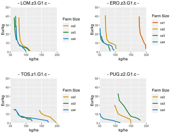
Figure 6.
Variations of the abatement costs at different CO2 emission levels by region and arable land size class. Regions: LOM = Lombardia, ERO = Emilia-Romagna, TOS = Toscana, PUG = Puglia; climates: Z1 = Lauretum, Z2 = Quercetum, Z3 = Castanetum; G1 = plain, G2 = mild slope, G3 = hilly; farming system: c = conventional, o = organic; arable land size classes: cs1 = <5 ha, cs2 = 5–15 ha, cs3 = 15–40 ha, cs4 = >40 ha.
Almost every curve shows S-shaped behaviour. Moving from BAU, abatement costs grow rapidly, and then reach a nearly stable value due to the existence of alternatives that preserve income. A further reduction in emissions corresponds to a dramatic MAC increase, particularly in the north.
Finally, the study shows that a reduction of CO2 emissions higher than 5 kg/ha, at an AC lower than 1 EUR/kg is affordable only in six s regions, among which ABR, and LOM show higher potential (Table 6).
Table 6.
Contexts with CO2 emissions higher than 5 kg/ha at an AC lower than 1 EUR/kg.
4. Discussion and Conclusions
The assessment of economic and environmental sustainability of agricultural systems represents a critical issue, which has been addressed in this work with an integrated approach based on the LMP to explore the abatement costs of CO2 for a set of representative contexts of Italian arable land agriculture.
The study has shown a quite diversified situation regarding income and emission levels per hectare across Italian regions and farm classes, due to diversified cropping systems and production processes. A more homogeneous situation emerged, considering the marginal abatement cost, which spanned 0–40 EUR/kg of CO2, but below EUR 1, emissions showed nearly no reduction.
ETS, introduced by EU policies to reduce industrial emissions, got a price raise in the last 10 years from 0.10 to 0.23 EUR/kg of CO2, and further increases are expected that could further increase the price to 0.4 EUR/kg of CO2.
Comparing ETS values to MACs in the agricultural systems taken into account highlighted a difference of 1 order of magnitude, which can probably be ascribed to the huge difference in efficiency between the industrial and agricultural production systems. Only in a few cases could relevant emission reductions be obtained at a cost lower than 1 EUR/kg. Therefore, to reduce emissions, innovation should be introduced in the arable cropping systems in terms of technologies with a lower use of resources, especially internal combustion engine machinery, and a general increase of energy efficiency.
The simulation and optimisation tool developed proved to produce insightful responses to estimated CO2 emissions and their abatement costs. It is important to highlight that this analysis was based on a short-term perspective. Therefore, it is useful to provide foresight on possible immediate impacts and contingency adjustments implemented by farmers in response to environmental policies to reduce emissions [45,46,47]. However, further research is necessary to complement this analysis and provide a medium to long-term perspective, in which structural adaptation on the supply side, such as land-use changes, technological innovation, intensification or extensification [48,49], supply chain adaptations, and market developments on the demand side, [50,51] are also allowed.
The FADN-compliant Italian RICA has been shown to collect information adequate to perform quantitative analysis of economical and agrotechnical aspects.
Data availability is at the base of statistical approaches adopted to derive technical parameters. An important contribution of this analysis lies in its reliance on actual farm accountancy data rather than simulation-based data. Such context-dependent parameters, describing production processes at a crop level, can be useful to other bio-economic models.
The model developed, designed to use RICA’s information solely and based on an innovative concept of a cropping scheme to simulate land-use adaptation, proved reliable and capable of conducting multi-criteria analysis.
Nonetheless, both the model and its background database can be improved. The model is ready to host more equations and constraints to study other farm contexts and consider other socio-economic and environmental criteria.
Several aspects can be enhanced in the RICA database to collect records that consistently refer to the same farm over the years, link to other databases, and enrich the information on non-conventional agricultural approaches (e.g., organic).
Further research may be addressed to update the analysis to more recent RICA surveys and introduce stakeholder perspectives. Collaborations with the RICA maintenance team and other national and international research and survey institutions could open further opportunities to develop the tool.
Author Contributions
Conceptualisation, G.V., G.M.B. and M.C.; methodology, G.M.B. and, G.V.; mathematical programming, G.M.B.; software, G.M.B. and G.V.; validation, G.V. and G.M.B.; data curation, C.C. and G.V.; resources, M.C.; writing—original draft preparation, G.V. and G.M.B.; writing—review and editing, M.C., G.M.B. and G.V.; visualisation, G.V.; funding acquisition, M.C. All authors have read and agreed to the published version of the manuscript.
Funding
This research was funded by the Italian Ministry of Agricultural, Food, and Forest Policies, project BIOSUS “Impatto dell’agricoltura biologica sulla sostenibilità ambientale e sulle emissioni di gas serra”, Bando Agricoltura biologica-D.M. 6553/2013.
Data Availability Statement
Restrictions apply to the availability of these data. The data were obtained from the Council for Agricultural Research and Economics (CREA) and are accessible at the URL https://bancadatirica.crea.gov.it/Account/Login.aspx with the permission of CREA.
Acknowledgments
We gratefully acknowledge the support of CREA for making the RICA data available to the research team.
Conflicts of Interest
The authors declare no conflict of interest. The funders had no role in the design of the study; in the collection, analyses, or interpretation of data; in the writing of the manuscript, or in the decision to publish the results.
Appendix A
| CONTEXT | FARM | SURF | CC | INC | CO2 | N | LAF | LAE | D.INC | D.CO2 | D.N | D.LAF | D.LAE | AC | cs |
| LOMcs1G2Z3 | 67 | 168 | 6 | 921 | 294 | 32 | 82.6 | 0 | cs1 | ||||||
| LOMcs1G2Z3 | 67 | 168 | 6 | 894 | 289 | 23 | 79.3 | 0 | −27.4 | −5.65 | −9.02 | −3.3 | 0 | 4.85 | cs1 |
| LOMcs2G1Z3 | 7814 | 39070 | 28 | 714 | 120 | 135 | 55.8 | 0 | cs2 | ||||||
| LOMcs2G1cZ3 | 7814 | 39070 | 28 | 710 | 117 | 133 | 54.8 | 0 | −3.7 | −2.29 | −2.05 | −0.92 | 0 | 1.616 | cs2 |
| LOMcs2G1Z4 | 101 | 503 | 12 | 2691 | 120 | 43 | 45.4 | 0 | cs2 | ||||||
| LOMcs2G1Z4 | 101 | 503 | 12 | 2684 | 117 | 43 | 44.8 | 0 | −6.35 | −3.12 | −0.12 | −0.63 | 0 | 2.035 | cs2 |
| LOMcs2G2Z3 | 1337 | 6683 | 19 | 1323 | 197 | 103 | 101.2 | 0 | cs2 | ||||||
| LOMcs2G2Z3 | 1337 | 6683 | 22 | 1318 | 192 | 89 | 100.4 | 0 | −4.97 | −4.43 | −14.46 | −0.8 | 0 | 1.122 | cs2 |
| LOMcs3G1Z3 | 4084 | 81683 | 51 | 995 | 111 | 138 | 56.3 | 3.4 | cs3 | ||||||
| LOMcs3G1Z3 | 4084 | 81683 | 51 | 995 | 110 | 137 | 56.2 | 3.4 | −0.29 | −0.12 | −1.11 | −0.11 | 0 | 2.417 | cs3 |
| LOMcs3G1Z4 | 138 | 2768 | 13 | 474 | 80 | 125 | 25.4 | 0 | cs3 | ||||||
| LOMcs3G1cZ4 | 138 | 2768 | 16 | 472 | 78 | 122 | 24.8 | 0 | −1.76 | −2.51 | −3.37 | −0.67 | 0 | 0.701 | cs3 |
| LOMcs3G2Z3 | 351 | 7014 | 11 | 553 | 100 | 157 | 61 | 0 | cs3 | ||||||
| LOMcs3G2Z3 | 351 | 7014 | 11 | 548 | 91 | 147 | 49.8 | 0 | −5.32 | −9.58 | −10.09 | −11.16 | 0 | 0.555 | cs3 |
| LOMcs4G1Z3 | 3891 | 155642 | 53 | 1063 | 96 | 157 | 37 | 17.1 | cs4 | ||||||
| LOMcs4G1Z3 | 3891 | 155642 | 53 | 1062 | 95 | 155 | 36.7 | 16.7 | −0.95 | −1.33 | −1.85 | −0.32 | −0.41 | 0.714 | cs4 |
| LOMcs4G1Z4 | 144 | 5746 | 12 | 73 | 151 | 204 | 38.9 | 0 | cs4 | ||||||
| LOMcs4G1Z4 | 144 | 5746 | 23 | 56 | 120 | 161 | 30.5 | 0 | −16.78 | −31.25 | −43.09 | −8.37 | 0 | 0.537 | cs4 |
| VENcs2G1Z3 | 10456 | 52279 | 53 | 420 | 221 | 46 | 65.1 | 0 | cs2 | ||||||
| VENcs2G1cZ3 | 10456 | 52279 | 53 | 419 | 217 | 44 | 63.9 | 0 | −0.42 | −4.1 | −1 | −1.22 | 0 | 0.102 | cs2 |
| VENcs2G1Z3 | 10456 | 52279 | 53 | 415 | 217 | 41 | 63.6 | 0 | −4.57 | −4.31 | −4.81 | −1.51 | 0 | 1.06 | cs2 |
| VENcs3G1Z3 | 2436 | 48723 | 20 | 126 | 198 | 48 | 48.9 | 0 | cs3 | ||||||
| VENcs3G1Z3 | 2436 | 48723 | 20 | 123 | 198 | 46 | 48.9 | 0 | −2.11 | −0.21 | −2.26 | −0.02 | 0 | 10.048 | cs3 |
| VENcs4G1Z3 | 1333 | 53313 | 54 | 427 | 167 | 50 | 32.8 | 18.4 | cs4 | ||||||
| VENcs4G1Z3 | 1333 | 53313 | 54 | 426 | 165 | 49 | 32.4 | 18.2 | −0.93 | −1.92 | −0.82 | −0.43 | −0.19 | 0.484 | cs4 |
| VENcs4G1Z3 | 1333 | 53313 | 54 | 422 | 162 | 46 | 31.7 | 18.2 | −5.42 | −4.91 | −3.32 | −1.12 | −0.16 | 1.104 | cs4 |
| EROcs1G1Z3 | 962 | 2406 | 19 | 3737 | 283 | 244 | 219.1 | 0 | cs1 | ||||||
| EROcs1G1cZ3 | 962 | 2406 | 21 | 3600 | 270 | 225 | 212.9 | 0 | −137.07 | −12.66 | −19.56 | −6.2 | 0 | 10.827 | cs1 |
| EROcs2G1Z3 | 8518 | 42588 | 52 | 1439 | 112 | 148 | 58.3 | 0 | cs2 | ||||||
| EROcs2G1Z3 | 8518 | 42588 | 46 | 1437 | 111 | 146 | 57.7 | 0 | −1.83 | −1.26 | −2.35 | −0.55 | 0 | 1.452 | cs2 |
| EROcs3G1Z3 | 5419 | 108374 | 47 | 1391 | 82 | 132 | 40.2 | 0.8 | cs3 | ||||||
| EROcs3G1Z3 | 5419 | 108374 | 53 | 1390 | 81 | 125 | 40 | 0.8 | −1.41 | −0.71 | −7.06 | −0.28 | 0.01 | 1.986 | cs3 |
| EROcs3G2Z3 | 394 | 7878 | 5 | 669 | 83 | 64 | 37.6 | 0 | cs3 | ||||||
| EROcs3G2Z3 | 394 | 7878 | 13 | 630 | 78 | 59 | 35.7 | 0 | −39.02 | −4.74 | −4.48 | −1.91 | 0 | 8.232 | cs3 |
| EROcs4G1Z3 | 5787 | 231460 | 53 | 1046 | 89 | 126 | 23.1 | 20.9 | cs4 | ||||||
| EROcs4G1cZ3 | 5787 | 231460 | 53 | 1046 | 88 | 125 | 23.1 | 20.3 | −0.13 | −1.19 | −1.39 | 0.02 | −0.54 | 0.109 | cs4 |
| EROcs4G1Z3 | 5787 | 231460 | 53 | 1043 | 87 | 124 | 23.1 | 20 | −2.76 | −1.95 | −2.72 | −0.02 | −0.89 | 1.415 | cs4 |
| EROcs4G2Z3 | 218 | 8711 | 6 | 1329 | 34 | 211 | 13.7 | 2.9 | cs4 | ||||||
| EROcs4G2Z3 | 218 | 8711 | 6 | 1324 | 32 | 210 | 13.7 | 2.3 | −5.04 | −1.51 | −1.52 | 0 | −0.64 | 3.338 | cs4 |
| EROcs4G3Z3 | 111 | 4432 | 5 | 1708 | 47 | 51 | 19.8 | 21.6 | cs4 | ||||||
| EROcs4G3Z3 | 111 | 4432 | 5 | 1706 | 44 | 48 | 19.8 | 21.2 | −2.24 | −2.08 | −2.99 | 0 | −0.41 | 1.077 | cs4 |
| MARcs2G3Z3 | 250 | 1250 | 7 | 391 | 74 | 106 | 30 | 0 | cs2 | ||||||
| MARcs2G3Z3 | 250 | 1250 | 7 | 312 | 57 | 78 | 24.9 | 0 | −79.31 | −16.39 | −27.43 | −5.1 | 0 | 4.839 | cs2 |
| MARcs3G1cZ3 | 432 | 8649 | 24 | 180 | 103 | 103 | 34.7 | 0 | cs3 | ||||||
| MARcs3G1Z3 | 432 | 8649 | 37 | 178 | 100 | 98 | 34 | 0 | −2.2 | −2.41 | −4.06 | −0.65 | 0 | 0.913 | cs3 |
| MARcs3G2Z3 | 819 | 16381 | 33 | 541 | 102 | 79 | 44.9 | 0 | cs3 | ||||||
| MARcs3G2Z3 | 819 | 16381 | 33 | 541 | 101 | 78 | 44.7 | 0 | −0.05 | −0.71 | −0.14 | −0.22 | 0 | 0.07 | cs3 |
| MARcs3G2Z3 | 819 | 16381 | 32 | 537 | 101 | 75 | 44.8 | 0 | −3.66 | −0.88 | −3.5 | −0.14 | 0 | 4.159 | cs3 |
| MARcs3G3Z3 | 108 | 2168 | 9 | 2319 | 225 | 366 | 68.2 | 92 | cs3 | ||||||
| MARcs3G3Z3 | 108 | 2168 | 15 | 2098 | 193 | 273 | 68.2 | 15.5 | −220.38 | −31.54 | −92.96 | 0 | −76.55 | 6.987 | cs3 |
| MARcs4G2Z3 | 223 | 8903 | 36 | 762 | 88 | 73 | 21.8 | 4.1 | cs4 | ||||||
| MARcs4G2cZ3 | 223 | 8903 | 41 | 761 | 86 | 70 | 21.8 | 3.6 | −0.31 | −1.8 | −2.76 | 0 | −0.51 | 0.172 | cs4 |
| MARcs4G2Z3 | 223 | 8903 | 36 | 759 | 86 | 69 | 21.7 | 3.6 | −2.25 | −1.9 | −3.85 | −0.07 | −0.52 | 1.184 | cs4 |
| MARcs4G3Z3 | 377 | 15070 | 22 | 545 | 90 | 93 | 29.9 | 0.2 | cs4 | ||||||
| MARcs4G3Z3 | 377 | 15070 | 23 | 544 | 89 | 92 | 29.9 | 0 | −0.52 | −0.52 | −0.83 | 0 | −0.15 | 1 | cs4 |
| TOScs2G1Z1 | 533 | 2666 | 14 | 1862 | 249 | 166 | 87.2 | 0 | cs2 | ||||||
| TOScs2G1Z1 | 533 | 2666 | 15 | 1862 | 249 | 166 | 87.1 | 0 | −0.01 | −0.18 | −0.06 | −0.06 | 0 | 0.056 | cs2 |
| TOScs2G1Z1 | 533 | 2666 | 30 | 1852 | 248 | 164 | 86.8 | 0 | −10.77 | −1.55 | −1.98 | −0.33 | 0 | 6.948 | cs2 |
| TOScs2G1Z3 | 353 | 1767 | 13 | 293 | 70 | 89 | 21.9 | 0 | cs2 | ||||||
| TOScs2G1cZ3 | 353 | 1767 | 13 | 293 | 70 | 88 | 21.8 | 0 | −0.24 | −0.36 | −0.69 | −0.06 | 0 | 0.667 | cs2 |
| TOScs3G1Z1 | 171 | 3413 | 35 | 2002 | 149 | 158 | 62.2 | 29.3 | cs3 | ||||||
| TOScs3G1Z1 | 171 | 3413 | 29 | 1978 | 149 | 142 | 62.2 | 25.6 | −24.52 | −0.12 | −15.46 | 0 | −3.76 | 204.333 | cs3 |
| TOScs3G2Z1 | 266 | 5312 | 31 | 25 | 50 | 19 | 15.7 | 0 | cs3 | ||||||
| TOScs3G2Z1 | 266 | 5312 | 31 | 25 | 50 | 19 | 15.7 | 0 | −0.02 | −0.03 | −0.02 | −0.01 | 0 | 0.667 | cs3 |
| TOScs3G2Z3 | 85 | 1699 | 21 | 95 | 59 | 38 | 93.5 | 0 | cs3 | ||||||
| TOScs3G2Z3 | 85 | 1699 | 20 | 81 | 58 | 30 | 66.2 | 0 | −14.21 | −1.53 | −7.98 | −27.32 | 0 | 9.288 | cs3 |
| TOScs3G3Z3 | 229 | 4572 | 17 | 146 | 78 | 41 | 23 | 0 | cs3 | ||||||
| TOScs3G3cZ3 | 229 | 4572 | 17 | 145 | 78 | 41 | 22.9 | 0 | −1.66 | −0.19 | −0.61 | −0.11 | 0 | 8.737 | cs3 |
| TOScs4G1Z1 | 474 | 18945 | 29 | 1274 | 169 | 183 | 28.4 | 51.2 | cs4 | ||||||
| TOScs4G1Z1 | 474 | 18945 | 37 | 1210 | 156 | 155 | 28.2 | 42.3 | −64.13 | −12.27 | −28.19 | −0.15 | −8.92 | 5.227 | cs4 |
| TOScs4G2Z1 | 269 | 10773 | 26 | 166 | 52 | 47 | 11.2 | 0.9 | cs4 | ||||||
| TOScs4G2Z1 | 269 | 10773 | 26 | 165 | 52 | 45 | 11 | 0.9 | −1.03 | −0.5 | −2.52 | −0.15 | 0 | 2.06 | cs4 |
| TOScs4G2Z3 | 409 | 16378 | 26 | 178 | 63 | 45 | 15.7 | 1.1 | cs4 | ||||||
| TOScs4G2Z3 | 409 | 16378 | 26 | 178 | 62 | 45 | 15.7 | 1.1 | −0.04 | −0.16 | −0.09 | −0.04 | 0 | 0.25 | cs4 |
| TOScs4G2Z3 | 409 | 16378 | 26 | 169 | 62 | 42 | 15.6 | 1.1 | −9.27 | −0.48 | −2.88 | −0.05 | −0.04 | 19.313 | cs4 |
| TOScs4G3cZ3 | 49 | 1977 | 18 | 87 | 81 | 35 | 21.3 | 0 | cs4 | ||||||
| TOScs4G3Z3 | 49 | 1977 | 18 | 82 | 74 | 30 | 19.5 | 0 | −5.34 | −6.79 | −5.59 | −1.85 | 0 | 0.786 | cs4 |
| ABRcs1G2Z3 | 305 | 763 | 18 | 711 | 198 | 52 | 154.1 | 0 | cs1 | ||||||
| ABRcs1G2Z3 | 305 | 763 | 18 | 711 | 198 | 52 | 154 | 0 | −0.25 | −0.29 | −0.11 | −0.1 | 0 | 0.862 | cs1 |
| ABRcs2G1Z3 | 439 | 2195 | 32 | 1100 | 240 | 52 | 169.8 | 0 | cs2 | ||||||
| ABRcs2G1Z3 | 439 | 2195 | 28 | 1100 | 240 | 52 | 169.4 | 0 | −0.19 | −0.71 | −0.17 | −0.4 | 0 | 0.268 | cs2 |
| ABRcs2G1Z3 | 439 | 2195 | 29 | 1072 | 234 | 48 | 166.6 | 0 | −28.56 | −6.32 | −4.02 | −3.28 | 0 | 4.519 | cs2 |
| ABRcs2G2Z1 | 42 | 211 | 24 | 861 | 226 | 23 | 108.2 | 0 | cs2 | ||||||
| ABRcs2G2cZ1 | 42 | 211 | 24 | 782 | 97 | 10 | 25.3 | 0 | −78.85 | −128.91 | −12.76 | −82.93 | 0 | 0.612 | cs2 |
| ABRcs2G2Z3 | 808 | 4042 | 38 | 509 | 163 | 37 | 99.4 | 0 | cs2 | ||||||
| ABRcs2G2Z3 | 808 | 4042 | 38 | 507 | 161 | 37 | 99.4 | 0 | −2.03 | −1.84 | −0.51 | −0.01 | 0 | 1.103 | cs2 |
| ABRcs3G1Z1 | 51 | 1026 | 10 | 836 | 148 | 61 | 50.1 | 13.7 | cs3 | ||||||
| ABRcs3G1Z1 | 51 | 1026 | 10 | 833 | 142 | 59 | 48.2 | 13.7 | −3.02 | −5.7 | −1.55 | −1.94 | 0 | 0.53 | cs3 |
| ABRcs3G2Z3 | 244 | 4873 | 37 | 2778 | 162 | 42 | 35.7 | 22.2 | cs3 | ||||||
| ABRcs3G2Z3 | 244 | 4873 | 37 | 2770 | 162 | 40 | 35.9 | 22.2 | −8.3 | −0.48 | −2.15 | 0.17 | 0 | 17.292 | cs3 |
| ABRcs4G2Z3 | 43 | 1740 | 37 | 339 | 115 | 30 | 11.1 | 26.9 | cs4 | ||||||
| ABRcs4G2cZ3 | 43 | 1740 | 37 | 193 | 89 | 21 | 11.1 | 18.2 | −145.74 | −26.47 | −8.23 | 0 | −8.62 | 5.506 | cs4 |
| LAZcs1G1Z2 | 421 | 1053 | 16 | 3929 | 106 | 36 | 553.2 | 0 | cs1 | ||||||
| LAZcs1G1Z2 | 421 | 1053 | 20 | 2976 | 90 | 25 | 481 | 0 | −952.32 | −16.26 | −10.5 | −72.22 | 0 | 58.568 | cs1 |
| LAZcs3G1Z1 | 430 | 8608 | 32 | 2479 | 134 | 16 | 112.9 | 68.2 | cs3 | ||||||
| LAZcs3G1Z1 | 430 | 8608 | 32 | 2478 | 134 | 16 | 112.9 | 68.2 | −0.38 | −0.27 | −0.05 | 0 | 0 | 1.407 | cs3 |
| LAZcs3G2Z3 | 980 | 19607 | 42 | 120 | 103 | 26 | 30.7 | 1.6 | cs3 | ||||||
| LAZcs3G2Z3 | 980 | 19607 | 41 | 114 | 103 | 25 | 30.1 | 1.6 | −5.48 | −0.69 | −1.07 | −0.66 | 0 | 7.942 | cs3 |
| LAZcs4G1Z1 | 806 | 32246 | 43 | 1283 | 52 | 19 | 26.7 | 51.4 | cs4 | ||||||
| LAZcs4G1cZ1 | 806 | 32246 | 43 | 1281 | 52 | 19 | 26.6 | 51.1 | −1.79 | −0.06 | −0.15 | −0.13 | −0.21 | 29.833 | cs4 |
| LAZcs4G2Z3 | 49 | 1941 | 12 | 181 | 65 | 76 | 15.7 | 0 | cs4 | ||||||
| LAZcs4G2Z3 | 49 | 1941 | 13 | 164 | 58 | 72 | 13.4 | 0 | −16.73 | −7 | −4.32 | −2.26 | 0 | 2.39 | cs4 |
| CAMcs2G1Z2 | 745 | 3723 | 27 | 2059 | 293 | 119 | 194.5 | 29.5 | cs2 | ||||||
| CAMcs2G1Z2 | 745 | 3723 | 31 | 2045 | 286 | 112 | 186 | 28.3 | −14.32 | −7.07 | −6.91 | −8.52 | −1.22 | 2.025 | cs2 |
| CAMcs2G1Z3 | 210 | 1050 | 23 | 1645 | 223 | 34 | 231.1 | 0 | cs2 | ||||||
| CAMcs2G1Z3 | 210 | 1050 | 16 | 1640 | 211 | 32 | 231.1 | 0 | −5.5 | −11.4 | −1.75 | 0 | 0 | 0.482 | cs2 |
| CAMcs2G1Z3 | 210 | 1050 | 28 | 1355 | 119 | 16 | 141.1 | 0 | −290.11 | −104 | −18.18 | −89.95 | 0 | 2.79 | cs2 |
| CAMcs2G2cZ3 | 800 | 4000 | 25 | 1231 | 83 | 21 | 307.8 | 0 | cs2 | ||||||
| CAMcs2G2Z3 | 800 | 4000 | 29 | 1229 | 80 | 20 | 305.8 | 0 | −1.42 | −2.34 | −1.39 | −2.04 | 0 | 0.607 | cs2 |
| CAMcs3G1Z1 | 195 | 3890 | 14 | 1875 | 72 | 74 | 49.9 | 34.4 | cs3 | ||||||
| CAMcs3G1Z1 | 195 | 3890 | 15 | 1806 | 40 | 60 | 35.6 | 34.4 | −69.2 | −31.89 | −14.58 | −14.38 | 0 | 2.17 | cs3 |
| CAMcs3G1Z3 | 296 | 5922 | 31 | 699 | 181 | 32 | 123.3 | 22.7 | cs3 | ||||||
| CAMcs3G1Z3 | 296 | 5922 | 33 | 689 | 178 | 31 | 122.6 | 22.7 | −9.47 | −2.6 | −1.22 | −0.73 | 0 | 3.642 | cs3 |
| CAMcs3G2Z3 | 159 | 3190 | 18 | 1147 | 99 | 47 | 85.3 | 10.8 | cs3 | ||||||
| CAMcs3G2Z3 | 159 | 3190 | 19 | 1145 | 98 | 45 | 84.8 | 10.8 | −1.78 | −0.91 | −1.55 | −0.59 | 0 | 1.956 | cs3 |
| CAMcs4G2cZ1 | 32 | 1261 | 11 | 3165 | 26 | 145 | 32.9 | 129.5 | cs4 | ||||||
| CAMcs4G2Z1 | 32 | 1261 | 11 | 2915 | 21 | 133 | 32.9 | 110.3 | −249.46 | −4.81 | −12.02 | 0 | −19.23 | 51.863 | cs4 |
| PUGcs2G1Z1 | 2184 | 10922 | 29 | 3719 | 162 | 40 | 135 | 122.2 | cs2 | ||||||
| PUGcs2G1Z1 | 2184 | 10922 | 29 | 3719 | 162 | 40 | 135 | 122.1 | −0.25 | −0.3 | −0.12 | 0 | −0.1 | 0.833 | cs2 |
| PUGcs2G1Z2 | 1459 | 7296 | 13 | 1692 | 177 | 76 | 91.9 | 17.9 | cs2 | ||||||
| PUGcs2G1Z2 | 1459 | 7296 | 25 | 1659 | 152 | 71 | 84.8 | 17.7 | −33.27 | −25.71 | −4.77 | −7.1 | −0.21 | 1.294 | cs2 |
| PUGcs2G1Z2 | 1459 | 7296 | 25 | 1572 | 146 | 61 | 82.9 | 17.7 | −86.75 | −5.96 | −10.62 | −1.78 | −0.0 | 14.555 | cs2 |
| PUGcs2G1Z2 | 1459 | 7296 | 25 | 1318 | 129 | 54 | 97.3 | 15.2 | −253.77 | −16.18 | −7.40 | 14.32 | −2.43 | 15.684 | cs2 |
| PUGcs2G1cZ2 | 1459 | 7296 | 25 | 678 | 104 | 53 | 29.9 | 14.5 | −640.08 | −25.59 | −0.69 | −67.46 | −0.77 | 25.013 | cs2 |
| PUGcs2G2Z3 | 366 | 1831 | 6 | 195 | 77 | 31 | 41.5 | 0 | cs2 | ||||||
| PUGcs2G2Z3 | 366 | 1831 | 6 | 195 | 77 | 31 | 41.3 | 0 | −0.11 | −0.69 | −0.13 | −0.21 | 0 | 0.159 | cs2 |
| PUGcs2G2Z3 | 366 | 1831 | 6 | 168 | 76 | 27 | 41.1 | 0 | −27.48 | −1.65 | −4.29 | −0.42 | 0 | 16.655 | cs2 |
| PUGcs3G1Z1 | 1081 | 21617 | 26 | 482 | 127 | 25 | 39.6 | 81.7 | cs3 | ||||||
| PUGcs3G1Z1 | 1081 | 21617 | 26 | 482 | 126 | 24 | 39.6 | 81.2 | −0.44 | −1.21 | −0.49 | 0 | −0.41 | 0.364 | cs3 |
| PUGcs3G1Z1 | 1081 | 21617 | 26 | 480 | 125 | 24 | 39.6 | 81 | −2.02 | −1.88 | −0.83 | 0 | −0.64 | 1.074 | cs3 |
| PUGcs3G1Z2 | 556 | 11112 | 13 | 1877 | 166 | 70 | 78.1 | 37.8 | cs3 | ||||||
| PUGcs3G1cZ2 | 556 | 11112 | 13 | 1822 | 163 | 65 | 76.7 | 37 | −55.62 | −2.72 | −5.76 | −1.38 | −0.84 | 20.449 | cs3 |
| PUGcs3G1Z3 | 1714 | 34275 | 26 | 511 | 81 | 47 | 39.5 | 0 | cs3 | ||||||
| PUGcs3G1Z3 | 1714 | 34275 | 26 | 505 | 79 | 46 | 39.2 | 0 | −5.65 | −1.29 | −1.06 | −0.32 | 0 | 4.38 | cs3 |
| PUGcs4G1Z1 | 738 | 29512 | 14 | 2142 | 231 | 50 | 28 | 121.3 | cs4 | ||||||
| PUGcs4G1Z1 | 738 | 29512 | 14 | 2141 | 230 | 49 | 28 | 120.7 | −0.75 | −1.54 | −0.84 | 0 | −0.57 | 0.487 | cs4 |
| PUGcs4G1Z1 | 738 | 29512 | 14 | 2140 | 229 | 49 | 28 | 120.6 | −1.57 | −1.88 | −1.02 | 0 | −0.69 | 0.835 | cs4 |
| PUGcs4G1Z3 | 306 | 12227 | 15 | 499 | 113 | 214 | 37.2 | 33.1 | cs4 | ||||||
| PUGcs4G1Z3 | 306 | 12227 | 15 | 498 | 111 | 213 | 37.2 | 32.6 | −1.91 | −2.07 | −1.7 | 0 | −0.51 | 0.923 | cs4 |
| PUGcs4G2cZ3 | 292 | 11681 | 11 | 408 | 71 | 58 | 28.8 | 0 | cs4 | ||||||
| PUGcs4G2Z3 | 292 | 11681 | 11 | 356 | 60 | 44 | 25.6 | 0 | −52.11 | −10.25 | −14.05 | −3.11 | 0 | 5.084 | cs4 |
| CALcs2G2Z1 | 508 | 2538 | 12 | 709 | 147 | 7 | 59.9 | 0 | cs2 | ||||||
| CALcs2G2Z1 | 508 | 2538 | 12 | 703 | 144 | 7 | 58.8 | 0 | −6.11 | −3.22 | −0.36 | −1.12 | 0 | 1.898 | cs2 |
| CALcs3G2Z1 | 371 | 7413 | 9 | 791 | 231 | 3 | 67.8 | 0 | cs3 | ||||||
| CALcs3G2Z1 | 371 | 7413 | 9 | 790 | 231 | 3 | 67.6 | 0 | −0.38 | −0.66 | −0.04 | −0.23 | 0 | 0.576 | cs3 |
References
- Ikerd, J.E. The need for a system approach to sustainable agriculture. Agric. Ecosyst. Environ. 1993, 46. [Google Scholar] [CrossRef]
- Sadok, W.; Angevin, F.; Bergez, J.É.; Bockstaller, C.; Colomb, B.; Guichard, L.; Reau, R.; Doré, T. Ex ante assessment of the sustainability of alternative cropping systems: Implications for using multi-criteria decision-aid methods. A review. Agron. Sustain. Dev. 2008, 28, 163–174. [Google Scholar] [CrossRef]
- European Union. Directive (EU) 2018/410 of the European Parliament and the Council of 14 March 2018 amending Directive 2003/87/EC to Enhance Cost-Effective Emission Reductions and Low-Carbon Investments, and Decision (EU) 2015/1814; European Union: Brussels, Belgium, 2018. [Google Scholar]
- Campbell, B.M.; Beare, D.J.; Bennett, E.M.; Hall-Spencer, J.M.; Ingram, J.S.I.; Jaramillo, F.; Ortiz, R.; Ramankutty, N.; Sayer, J.A.; Shindell, D. Agriculture production as a major driver of the earth system exceeding planetary boundaries. Ecol. Soc. 2017, 22. [Google Scholar] [CrossRef]
- Niemeijer, D.; de Groot, R.S. A conceptual framework for selecting environmental indicator sets. Ecol. Indic. 2008, 8, 14–25. [Google Scholar] [CrossRef]
- Ness, B.; Urbel-Piirsalu, E.; Anderberg, S.; Olsson, L. Categorising tools for sustainability assessment. Ecol. Econ. 2007, 60, 498–505. [Google Scholar] [CrossRef]
- EEA Environmental Indicators: Typology and Overview—Technical Report No 25; European Environment Agency: København, Denmark, 1999.
- Latruffe, L.; Diazabakana, A.; Bockstaller, C.; Desjeux, Y.; Finn, J.; Kelly, E.; Ryan, M.; Uthes, S. Measurement of sustainability in agriculture: A review of indicators three sustainability pillars. Stud. Agric. Econ. 2016, 118, 123–130. [Google Scholar] [CrossRef]
- Deytieux, V.; Munier-Jolain, N.; Caneill, J. Assessing the sustainability of cropping systems in single- and multi-site studies. A review of methods. Eur. J. Agron. 2016, 72, 107–126. [Google Scholar] [CrossRef]
- Smith, C.; McDonald, G. Assessing the sustainability of agriculture at the planning stage. J. Environ. Manag. 1998, 52, 15–37. [Google Scholar] [CrossRef]
- Gómez-Limón, J.A.; Sanchez-Fernandez, G. Empirical evaluation of agricultural sustainability using composite indicators. Ecol. Econ. 2010, 69. [Google Scholar] [CrossRef]
- Romano, D.; Arcarese, C.; Bernetti, A.; Caputo, A.; Cordella, M.; De Lauretis, R.; Di Cristofaro, E.; Gagna, A.; Gonella, B.; Moricci, F.; et al. Italian Greenhouse Gas Inventory 1990–2019. National Inventory Report 2021. Annual Report for Submission under the UN Framework Convention on Climate Change and the Kyoto Protocol, ISPRA, Rapporti 341/21; ISPRA-Institute for Environmental Protection and Research: Rome, Italy, 2021; ISBN 9788844810467.
- Coderoni, S.; Bonati, G.; D’Angelo, L.; Longhitano, D.; Mambella, M.; Papaleo, A.; Vanino, S. Using FADN data to estimate agricultural GHG emissions at farm level. In Pacioli 20—Complex Farms and Sustainability in Farm Level Data Collection; Vrolijk, H., Ed.; LEI Wageningen UR: The Hague, The Netherlands, 2013; pp. 86–102. ISBN 978-90-8615-634-4. [Google Scholar]
- Baldoni, E.; Coderoni, S.; Esposti, R. The productivity and environment nexus with farm-level data. The case of carbon footprint in lombardy fadn farms. Bio-Based Appl. Econ. 2017, 6, 119–137. [Google Scholar] [CrossRef]
- Baldoni, E.; Coderoni, S.; Esposti, R. The complex farm-level relationship between environmental performance and productivity: The case of carbon footprint of Lombardy farms. Environ. Sci. Policy 2018, 89, 73–82. [Google Scholar] [CrossRef]
- Diazabakana, A.; Latruffe, L.; Bockstaller, C.; Desjeux, Y.; Finn, J.; Kelly, E.; Ryan, M.; Uthes, S. A Review of Farm Level Inficators of Sustentability with a Focus on Cap and Fadn about the FLINT Project—FLINT Farm Level Indicators for New Topics in Policy Evaluation; European Commission: Brussels, Belgium, 2014. [Google Scholar]
- Gocht, A.; Espinosa, M.; Leip, A.; Lugato, E.; Schroeder, L.A.; Van Doorslaer, B.; Paloma, S.G.y. A grassland strategy for farming systems in Europe to mitigate GHG emissions—An integrated spatially differentiated modelling approach. Land Use Policy 2016, 58, 318–334. [Google Scholar] [CrossRef]
- Gocht, A.; Ciaian, P.; Bielza, M.; Terres, J.M.; Röder, N.; Himics, M.; Salputra, G. EU-wide Economic and Environmental Impacts of CAP Greening with High Spatial and Farm-type Detail. J. Agric. Econ. 2017, 68, 651–681. [Google Scholar] [CrossRef]
- Westbury, D.B.; Park, J.R.; Mauchline, A.L.; Crane, R.T.; Mortimer, S.R. Assessing the environmental performance of English arable and livestock holdings using data from the Farm Accountancy Data Network (FADN). J. Environ. Manag. 2011, 92, 902–909. [Google Scholar] [CrossRef]
- Coderoni, S.; Esposti, R. CAP payments and agricultural GHG emissions in Italy. A farm-level assessment. Sci. Total Environ. 2018, 627, 427–437. [Google Scholar] [CrossRef] [PubMed]
- Bonfiglio, A.; Arzeni, A.; Bodini, A. Assessing eco-efficiency of arable farms in rural areas. Agric. Syst. 2017, 151, 114–125. [Google Scholar] [CrossRef]
- Coluccia, B.; Valente, D.; Fusco, G.; De Leo, F.; Porrini, D. Assessing agricultural eco-efficiency in Italian Regions. Ecol. Indic. 2020, 116. [Google Scholar] [CrossRef]
- Syp, A.; Osuch, D. Assessing greenhouse gas emissions from conventional farms based on the farm accountancy data network. Polish J. Environ. Stud. 2018, 27, 1261–1268. [Google Scholar] [CrossRef]
- Greening, L.A.; Bernow, S. Design of coordinated energy and environmental policies: Use of multi-criteria decision-making. Energy Policy 2004, 32. [Google Scholar] [CrossRef]
- Energy Decisions and the Environment; Hobbs, B.F., Meier, P., Eds.; International Series in Operations Research & Management Science; Springer US: Boston, MA, USA, 2000; Volume 28, ISBN 978-1-4613-7017-8. [Google Scholar]
- Weintraub, A.; Romero, C. Operations Research Models and the Management of Agricultural and Forestry Resources: A Review and Comparison. Interfaces 2006, 36, 446–457. [Google Scholar] [CrossRef]
- Hayashi, K. Multicriteria analysis for agricultural resource management: A critical survey and future perspectives. Eur. J. Oper. Res. 2000, 122, 486–500. [Google Scholar] [CrossRef]
- Zeleny, M. Linear Multiobjective Programming; Lecture Notes in Economics and Mathematical Systems; Springer: Berlin/Heidelberg, Germany, 1974; Volume 95, ISBN 978-3-540-06639-2. [Google Scholar]
- Gunantara, N. A review of multi-objective optimisation: Methods and its applications. Cogent Eng. 2018, 5, 1502242. [Google Scholar] [CrossRef]
- Zeleny, M. Compromise Programming. In Multiple Criteria Decision Making; Cochrane, J., Zeleny, M., Eds.; University of South Carolina Press: Columbia, SC, USA, 1973; pp. 262–301. [Google Scholar]
- Todman, L.C.; Coleman, K.; Milne, A.E.; Gil, J.D.B.; Reidsma, P.; Schwoob, M.-H.; Treyer, S.; Whitmore, A.P. Multi-objective optimisation as a tool to identify possibilities for future agricultural landscapes. Sci. Total Environ. 2019, 687, 535–545. [Google Scholar] [CrossRef] [PubMed]
- Zander, P.; Kächele, H. Modelling multiple objectives of land use for sustainable development. Agric. Syst. 1999, 59, 311–325. [Google Scholar] [CrossRef]
- Pacini, C.; Wossink, A.; Giesen, G.; Huirne, R. Ecological-economic modelling to support multi-objective policy making: A farming systems approach implemented for Tuscany. Agric. Ecosyst. Environ. 2004, 102, 349–364. [Google Scholar] [CrossRef]
- Estes, L.D.; Searchinger, T.; Spiegel, M.; Tian, D.; Sichinga, S.; Mwale, M.; Kehoe, L.; Kuemmerle, T.; Berven, A.; Chaney, N.; et al. Reconciling agriculture, carbon and biodiversity in a savannah transformation frontier. Philos. Trans. R. Soc. B Biol. Sci. 2016, 371, 20150316. [Google Scholar] [CrossRef]
- Coleman, K.; Muhammed, S.E.; Milne, A.E.; Todman, L.C.; Dailey, A.G.; Glendining, M.J.; Whitmore, A.P. The landscape model: A model for exploring trade-offs between agricultural production and the environment. Sci. Total Environ. 2017, 609, 1483–1499. [Google Scholar] [CrossRef]
- Ditzler, L.; Komarek, A.M.; Chiang, T.-W.; Alvarez, S.; Chatterjee, S.A.; Timler, C.; Raneri, J.E.; Carmona, N.E.; Kennedy, G.; Groot, J.C.J. A model to examine farm household trade-offs and synergies with an application to smallholders in Vietnam. Agric. Syst. 2019, 173, 49–63. [Google Scholar] [CrossRef]
- Canavari, M.; Cantore, N.; Albertazzi, S.; Della Chiara, M.; Vitali, G.; Signorotti, C.; Baldoni, G.; Cardillo, C.; Trisorio, A.; Bazzani, G.M.; et al. Sustainability in organic and conventional farming: Towards a multicriteria model based on simulated farm indicators. Econ. Policy Energy Environ. 2013, 175–200. [Google Scholar] [CrossRef]
- Ballin, M.; Barcaroli, G. Joint determination of optimal stratification and sample allocation using genetic algorithm. Surv. Methodol. 2013, 39, 369–393. [Google Scholar]
- Bussieck, M.R.; Meeraus, A. General Algebraic Modeling System (GAMS). In Modeling Languages in Mathematical Optimization; Springer: Boston, MA, USA, 2004; pp. 137–157. [Google Scholar]
- Tomaselli, R.; Balduzzi, A.; Filipello, S. Carta Bioclimatica d’Italia; Ministero dell’agricoltura e delle Foreste: Roma, Italy, 1973. [Google Scholar]
- Pedrotti, F. Plant and Vegetation Mapping; Springer: Berlin/Heidelberg, Germany, 2013; ISBN 978-3-642-30234-3. [Google Scholar]
- Vitali, G.; Cardillo, C.; Albertazzi, S.; Della Chiara, M.; Baldoni, G.; Signorotti, C.; Trisorio, A.; Canavari, M. Classification of Italian farms in the FADN database combining climate and structural information. Cartographica 2012, 47, 228–236. [Google Scholar] [CrossRef]
- European Union. Regulation (EU) No 1307/2013. Establishing Rules for Direct Payments to Farmers under Support Schemes within the Framework of the Common Agricultural Policy; European Union: Brussels, Belgium, 2013. [Google Scholar]
- R Core Team. R: A Language and Environment for Statistical Computing; R Foundation for Statistical Computing: Vienna, Austria, 2020. [Google Scholar]
- Cortignani, R.; Dell’Unto, D.; Dono, G. Paths of adaptation to climate change in major Italian agricultural areas: Effectiveness and limits in supporting the profitability of farms. Agric. Water Manag. 2021, 244, 106433. [Google Scholar] [CrossRef]
- Bindi, M.; Olesen, J.E. The responses of agriculture in Europe to climate change. Reg. Environ. Chang. 2011, 11, 151–158. [Google Scholar] [CrossRef]
- Concu, G.B.; Atzeni, G.; Meleddu, M.; Vannini, M. Policy design for climate change mitigation and adaptation in sheep farming: Insights from a study of the knowledge transfer chain. Environ. Sci. Policy 2020, 107, 99–113. [Google Scholar] [CrossRef]
- Olesen, J.E.; Bindi, M. Consequences of climate change for European agricultural productivity, land use and policy. Eur. J. Agron. 2002, 16, 239–262. [Google Scholar] [CrossRef]
- Medici, M.; Canavari, M.; Toselli, M. Interpreting Environmental Impacts Resulting from Fruit Cultivation in a Business Innovation Perspective. Sustainability 2020, 12, 9793. [Google Scholar] [CrossRef]
- Canavari, M.; Coderoni, S. Green marketing strategies in the dairy sector: Consumer-stated preferences for carbon footprint labels. Strateg. Chang. 2019, 28, 233–240. [Google Scholar] [CrossRef]
- Canavari, M.; Coderoni, S. Consumer stated preferences for dairy products with carbon footprint labels in Italy. Agric. Food Econ. 2020, 8. [Google Scholar] [CrossRef]


Publisher’s Note: MDPI stays neutral with regard to jurisdictional claims in published maps and institutional affiliations. |
© 2021 by the authors. Licensee MDPI, Basel, Switzerland. This article is an open access article distributed under the terms and conditions of the Creative Commons Attribution (CC BY) license (https://creativecommons.org/licenses/by/4.0/).