Abstract
This paper investigates the optimal congestion pricing problem that considers day-to-day evolutionary flow dynamics. Under the circumstance that traffic flows evolve from day to day and the system might be in a non-equilibrium state during a certain period of days after implementing (or adjusting) a congestion toll scheme, it is questionable to use an equilibrium-based index under steady state as the objective to measure the performance of a congestion toll scheme. To this end, this paper proposes a mean–variance-based congestion pricing scheme, which is a robust optimization model, to consider the evolution process of traffic flow dynamics in the optimal toll design problem. More specifically, in the mean–variance-based toll scheme, travelers aim to minimize the variance of expected total travel costs (ETTCs) on different days to reduce risk in daily travels, while the average ETTC over the whole planning period is restricted to being no larger than a predetermined target value set by the authorities. A metaheuristic approach based on the whale optimization algorithm is designed to solve the proposed mean–variance-based day-to-day dynamic congestion pricing problem. Finally, a numerical experiment is conducted to validate the effectiveness of the proposed model and solution algorithm. Results show that the used 9-node network can reach a steady state within 18 days after implementing the mean–variance-based congestion pricing, and the optimal toll scheme can be also obtained with this toll strategy.
1. Introduction
Congestion exists in many network systems when demand temporarily and spatially exceeds capacity. Many regional planning organizations and transportation management authorities face enormous challenges in mitigating heavy traffic congestion to enable a high level of services for citizens. According to the Federal Highway Administration (FHWA) of the US [1], the budget request for fiscal year 2019 for transportation infrastructure capacity construction reached USD 40.41 billion; in 2018, traffic congestion cost Americans approximately USD 1348 per driver or USD 87 billion in total [2]. Similarly, many emerging mega-regions in Asia have invested substantially into road and transit backbone networks [3,4,5,6]. For example, the related budget in Beijing reached up to CNY 43.10 billion in 2018, but it is still very challenging to manage and spread the 36% of trips during the morning and afternoon peak hours (07:00~09:00 and 17:00~19:00); the current average speed of privately owned vehicles is 20 km/h [7]. It is widely recognized that only increasing infrastructure construction cannot fundamentally solve the traffic congestion problem, e.g., Braess’s paradox shows that an extension of the road network may deteriorate the overall network performance with the same traffic demand [8,9].
Congestion pricing, as a demand side traffic management scheme, is one of the most effective means to manage demand and relieve traffic congestion in urban central areas. It has been verified to be effective for easing congestion (and reducing emissions) in many cities, e.g., the Electronic Road Pricing (ERP) in Singapore [10], the Congestion Charge Zone (CCZ) in London [11], the Ecopass and Area C in Milan [12], and the congestion charge in Stockholm [13]. For a comprehensive review on congestion pricing, readers are referred to [14,15,16,17,18], etc. When measuring the performance of one particular congestion pricing scheme, the system’s total travel cost (TTC) is one of the most widely used indices to be minimized in the objective function. However, as already mentioned in [19], almost all existing studies calculate the TTC and evaluate the toll scheme in terms of equilibrium flow at steady state. This may be unreasonable since network flow cannot reach equilibria overnight after implementing a new toll scheme. Therefore, it is of great significance to take the day-to-day (DTD) dynamics evolution process of traffic flows into consideration in the congestion pricing problem.
Regarding the congestion pricing problem with DTD dynamics, some scholars, e.g., Wie and Tobin [20] formulated it as a convex optimal control model. Considering travelers’ route choice, learning, and adjustment process, Sandholm [21] designed a dynamic toll scheme to make the whole network approach the system optimal state. Friesz et al. [22] formulated the day-to-day dynamic congestion pricing (DTD-DCP) problem to maximize the net present value of social benefits with a continuous time optimal control model, which can also account for elastic nonseparable traffic demands and nonseparable travel costs. Yang and Szeto [23] considered the rational behavior adjustment process in travelers’ route choice with DTD dynamics and designed a marginal-cost-based DCP scheme to achieve system optimal. Yang et al. [24] investigated the steepest descent scheme with DTD-DCP to force the system to evolve to the system optimal stationary state. Afterwards, Yang [25] extended the fixed demand DTD-DCP problem to an elastic demand case. Based on the bounded rationality theory, Guo [26] designed a toll sequence operation with DTD dynamics to make network flows evolve to the user equilibrium pattern. Considering network resilience, which measures the rapidity with which a network recovers to its normal state after a disruption, Wang et al. [27] proposed a DTD-DCP scheme to increase the rapidity of the network recovery process after disruptions. Ma et al. [28] investigated the DTD-DCP problem with a bi-objective optimization model, which takes into consideration travel time and monetary cost separately in the objective.
Guo et al. [29] designed a DCP scheme to control traffic flows evolving toward a predetermined upper bound of flows. The charge for each day is obtained from the toll and link flows on the previous day and the predetermined target of link flows. However, as pointed out in [30], the abovementioned DTD-DCP schemes either require the explicit mechanisms of the flow evolution process or the tolls should be adjustable to accommodate the change of network flows. To solve these drawbacks, Ye et al. [30] proposed a marginal-cost pricing scheme, which incorporates the DTD dynamics into the trial-and-error procedure without knowing the demand functions and flow evolution mechanisms. Xu et al. [31] also investigated the DTD-DCP problem with the trial-and-error method [32] based on observed disequilibrium flows, and the global convergence of the proposed method is verified without an explicit DTD dynamics model. The dynamic toll is piecewise-constant in [30], while it can be adjusted at any arbitrary time interval in [31]. Tan et al. [33] investigated the DCP problem with DTD dynamics and user heterogeneity, which is captured by the value of times. The DTD evolution trajectory is controlled by the dynamic toll scheme to simultaneously minimize system cost and travel time with the Pareto optimality concept.
Most of the existing DTD-DCP schemes [30,31,33,34] only focus on deterministic dynamics. By contrast, Gehlot et al. [35] proposed an optimal control approach with the Markov decision process for the DTD-DCP problem which incorporates demand uncertainty and elasticity. Liu et al. [19] investigated stochastic DTD dynamics and proposed a robust optimization model to determine the distance-based toll rate over a given planning period. Compared with the toll schemes in [30,31], the toll rate in [19] is fixed over the entire planning period (which is three months in their work), and the network performance of each day is taken into consideration in robust optimization with the objective of minimizing the maximum regret on each day. However, as shown in its objective function, one needs to first solve the optimal toll for each day and take the corresponding total travel cost as a benchmark for each day. It is obvious that calculating the optimal toll for each day over the whole planning period is very time-consuming in the first stage of the minimax model, and this paper proposes a new toll scheme to overcome the computational issues in the robust optimization minimax model proposed by [19] with DTD dynamics.
In this paper, we aim to design and solve the DTD-DCP problem in the mean–variance-based framework. Mean–variance analysis is widely used in financial economics to help investors to spread risk in the portfolio [36,37]. In mean–variance analysis, investors first measure risk, which is expressed by variance, and then compare the risk of an asset with its likely return. The aim of mean–variance optimization is to maximize the reward of an investment with respect to its risk. In the congestion pricing problem with DTD dynamics, the total travel cost for each day over the whole planning period changes from day to day, and there is not one particular toll scheme that can result in minimal total travel cost for each day. In the mean–variance-based toll scheme proposed in this paper, travelers aim to minimize the variance of expected total travel costs (ETTCs) on different days to reduce risk in daily travels, while the average ETTC over the whole planning period is restricted to being no larger than a predetermined target value set by the authorities to maximize the reward over the whole planning period. To solve the proposed mean–variance-based DTD-DCP problem, this paper designs a metaheuristic approach based on the whale optimization algorithm (WOA) [38].
The rest of this paper is organized as follows: Section 2 defines the notations used in this paper and describes the distance-based congestion pricing problem, which is a usage-oriented toll scheme and widely used in the literature (e.g., [19,39]; just to name a few). Section 3 describes the discrete route-based DTD dynamics model to capture the flow and cost evolution process. In the DTD dynamics model, the information provided by advanced traveler information systems (ATIS) is also taken into consideration. The mean–variance-based congestion pricing model to determine the robust optimal toll rate in the context of DTD dynamics is also demonstrated in Section 3 and followed by the WOA-based metaheuristic solution approach in Section 4. Finally, the numerical experiment and conclusions are outlined in Section 5 and Section 6, respectively.
2. Preliminaries
Consider a directed traffic network , where and are the set of nodes and links in the network, and and are the elements in and , respectively. Denote the set of origin–destination (OD) pairs by , and . The number of OD pairs is denoted by . is the path connecting OD pair , is its set, and is the number of paths connecting OD pair . is the traffic demand between OD pair . The flow and travel time on link are denoted by and . The flow on path is expressed by . The actual (i.e., experienced) path travel time for is denoted by . There are two types of forecasted travel time for path , including the path travel time forecasted by travelers and the path travel time forecasted by ATIS . The generalized path travel cost for is expressed by . represents the evolutionary calendar days for the DTD dynamics model, and is the total planning period of interest. The notations used in this paper are summarized in Table 1.

Table 1.
Notation and explanations.
The relationship between path travel time and link travel time can be expressed by
where if link is on path , which connects the OD pair , and otherwise. Taking congestion charging into consideration, we can calculate the generalized path travel cost by
where denotes the toll for path , and is the value of time (VOT), which is assumed to be a constant in this paper. It is worth noting that this constant VOT can be easily extended to a continuously distributed VOT [39], which is out of scope in this paper.
The congestion toll is assumed to be a distance-based scheme, which has recently attracted a lot of attention both theoretically [19,39,40,41] and practically [42]. Suppose that there is a charging cordon, which is predetermined by the government, in the transport network. For a particular path in the network connecting an OD pair , a portion of the path is located inside the charging cordon, with the length of . The toll function for using tolled roads inside the cordon is denoted by . Followed by [19,40], we use a piecewise linear toll function to approximate the nonlinear distance-based toll.
As illustrated in Figure 1a, the purple path connects a particular origin and destination pair. The charging cordon is shown in the dashed area, and the travel distance inside the cordon is calculated as 16.2, which is the sum of all link lengths belonging to the path inside the cordon. For a piecewise linear approximated toll scheme, we need to first define the minimal and maximal travel distances inside the cordon, which are denoted by and , with Z equal intervals between them. The toll values corresponding to are expressed by . As shown in Figure 1b, the toll with a travel distance of inside the cordon is calculated by
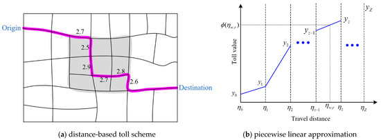
Figure 1.
Illustration of the distance-based toll scheme and its piecewise linear approximation [19,40].
With a determined toll scheme at the beginning of the planning period, the network flow will evolve dynamically from day to day. In the next section, we introduce a discrete DTD dynamics model to describe the DTD evolutionary flow dynamics.
3. Mathematical Formulations
3.1. A Discrete DTD Dynamics Model
After implementing a toll scheme, network flows will change since travelers’ route choice decisions will change due to the toll. Therefore, a toll levied in the charging cordon results in a new flow evolution trajectory. To evaluate the new toll scheme prior to implementation, one needs to make a prediction on the DTD flow evolution trajectory if this new toll scheme is implemented. In the DTD dynamics model, travelers make predictions on travel costs for the next day at the end of each day and then make decisions on the route choice behaviors in terms of the predicted route costs and previously experienced route costs.
In this paper, the ATIS is taken into consideration in travelers’ cost predictions [43]. In other words, at the end of day , the ATIS makes a prediction and broadcasts the predicted information (i.e., the route travel costs) through learning from the actual route travel costs and predicted route travel costs on day . In addition to the ATIS’s prediction, travelers also have their predictions on travel costs. With the information published by the ATIS, travelers predict the route travel costs by learning from the ATIS’s information and their predictions on the previous day. Finally, travelers make decisions in terms of their predictions. Mathematically, the DTD dynamics model can be expressed by the following three processes, i.e., the flow updating, cost updating, and information broadcasting processes:
[Flow Updating Process]
[Cost Updating Process]
[Information Broadcasting Process]
where , , and are the actual (i.e., experienced) route travel cost, the ATIS’s predicted route travel cost, and the traveler’s predicted route travel cost for on day , respectively. is the flow on route on day , and is the route choice probability function with respect to the predicted route travel cost based on the random utility theory. , , and are the flow updating parameter, traveler’s predicting parameter, and ATIS’s predicting parameter, respectively.
In this paper, it is assumed that the route choice probability function follows the logit model, giving
where is a perception-error-related parameter, which describes the dispersion in travelers’ route choices.
It is worth noting that when , we have , which means that ATIS’s prediction on the route travel cost for day at the end of day equals the actual travel cost experienced by travelers on day . In other words, the ATIS releases the actual travel cost at the end of each day when , and this is widely used in the DTD dynamics model [19,44,45].
3.2. Mean–Variance-Based Robust Optimization Model
Mean–variance analysis is one of the most important aspects of modern portfolio theory [46], and it is a process to weigh risk (which is expressed by the variance) against the expected return. Investors weigh how much risk they can take on in return for rewards. It is assumed that investors will rationally make decisions on investment if complete information is provided to them. In mean–variance analysis, investors seek to find the maximal reward under a given level of risk (or the minimal risk under a given level of reward).
As for the congestion pricing problem with DTD dynamics, the system-level performance measure with the total travel cost is fluctuant due to evolutionary traffic flow dynamics. It would be unlikely for one particular toll scheme to exist which results in a minimal total travel cost for each day over the whole planning period. Similar to the mean–variance analysis in the portfolio theory which minimizes the risk at a given level of reward, in the mean–variance-based toll scheme proposed in this paper, travelers aim to minimize the variance of total travel costs on different days, while the mean of the total travel costs over the whole planning period is restricted to being no larger than a predetermined target value set by the authorities. Additionally, since travelers experience perception errors in route choices, it is more reasonable to use the expected total travel costs (ETTCs) than the total travel cost in the objective function [19,41]. Mathematically, the expected total travel cost for each day under the toll scheme can be formulated as [19,41]:
where and are the column vectors of route flows and costs on day under toll scheme , respectively.
Therefore, in order to minimize risk, travelers seek to minimize the variance of expected total travel costs on different days with congestion pricing considering DTD traffic flow dynamics. Mathematically, this is expressed as
subject to
and the DTD dynamic traffic flows introduced in Section 3. is the expected total travel cost on day with toll scheme . is the predetermined target of the mean of expected total travel costs during the total planning period.
Objective (9) aims to minimize risk, while constraint (10) indicates that the reward should be no less than a given level (or, more strictly speaking, the negative reward should be no larger than a given level, since the expected total travel cost can be seen as the negative reward). Comparing the mean–variance-based toll scheme defined in Equations (9) and (10) with the minimax regret model in [19], we can see that it does not need to calculate the minimal ETTC for each day in the mean–variance-based toll scheme, which greatly reduces the computational burden in the solution procedure.
4. Solution Algorithms
With a particular toll rate, one needs to calculate the flow and cost evolutionary trajectories to obtain the objective value defined in Equation (9); obviously, this is difficult since there is no analytical formula for the objective function, and traditional gradient-based algorithms cannot be used to solve the complex model. In this paper, we propose a metaheuristic approach based on the whale optimization algorithm to solve the mean–variance-based congestion pricing problem under DTD dynamics.
The whale optimization algorithm is a nature-inspired metaheuristic algorithm which imitates the hunting behavior of humpback whales, including three operators of search for prey (i.e., exploration phase), encircling prey, and bubble-net foraging (i.e., exploitation phase). It was first proposed by [38]. Since then, it has attracted extensive attention and been widely used in many engineering optimization problems, e.g., classification, clustering, image processing, robot routing, and task scheduling; see a comprehensive review in [47]. As shown in [38], the whale optimization algorithm was found to be very competitive compared to other state-of-the-art metaheuristic algorithms with 29 mathematical benchmark functions and 6 structural engineering problems.
While it is popular in many engineering optimization problems, only a few studies [48,49] have solved traffic and transportation problems with the whale optimization algorithm. In this study, the whale optimization algorithm is used to solve the mean–variance-based congestion toll problem with DTD dynamics. One of the reasons that we chose the whale optimization algorithm is that it has an excellent ability to escape from local minima to find the global minima due to cooperation between the exploration and exploitation phases. The primary algorithm procedures are summarized as follows, while the details on the algorithm can be found in [38].
4.1. Encircling Prey
In the whale optimization algorithm, it is assumed that the current solution (i.e., the best search agent) is the target prey or close to the target prey, and other search agents update their locations toward the best search agent. Mathematically, this behavior can be formulated as:
where t is the iteration number, is the current best solution, is the vector of position, and are vectors of coefficients, and is an element-by-element multiplication. During the iteration process, will be updated continuously in each iteration if a better solution is obtained. The vectors of coefficients and can be calculated by:
where decreases linearly from two to zero, and is a random vector between zero and one.
4.2. Bubble-Net Attacking
A bubble-net strategy is used by whales to attack their prey. There are two approaches in the bubble-net strategy, the shrinking encircling mechanism and spiral updating position.
(1) Shrinking encircling mechanism
The location of the whale group is updated in terms of Equation (12). The values of are randomly set at [−1, 1], and the updated location of the search agent can be defined between its original location and the location of the current best solution.
(2) Spiral updating position
The whale moves along the spiral route in a shrinking circle, and this process can be mathematically formulated by:
where is the distance from individual whales to the whale with the best location so far. is a constant which determines the shape of the logarithmic spiral, and is a random value in [−1, 1]. The shrinking encircling and spiral updating strategies are performed simultaneously. In practical applications, we usually assume that there is a probability of 50% to select one of the shrinking encircling or spiral updating approaches to update the locations of whales [38]. This process can be summarized as follows:
where is a randomly generated value of [0, 1].
4.3. Search for Prey
Humpback whales hunt randomly for prey. In the whale optimization algorithm, the behavior of randomly searching for prey is based on the variation of . More specifically, the randomly chosen search agent will move far away from a reference whale when and move toward the whale with the best location so far when . Such a mechanism with a randomly chosen search agent (rather than the agent with the best solution) allows the whale optimization algorithm to perform a global search. Mathematically, the search for prey can be modeled as follows:
where is the random location (i.e., a random selected whale) chosen from the present population.
The pseudo code of the whale optimization algorithm can be summarized as follows [38]:
| Algorithm 1. |
| Initialize the population |
| Calculate the distance-based toll for each path with Equation (3) |
| Conduct the day-to-day dynamics evolution process with Equations (4)–(7) |
| Evaluate the fitness for all the agents in the population with Equation (9), and set as the best search agent |
| while (t < maxIterations): |
| for each search agent |
| update , , , l and p |
| if (p < 0.5): |
| if (): |
| update the location of the present search agent by Equation (11) |
| else if (): |
| randomly select a search agent |
| update the location of the randomly selected agent with Equation (18) |
| end if |
| else if (p 0.5): |
| update the location of the present search agent with Equation (15) |
| end if |
| Calculate the toll value for each path with Equation (3) for each search agent |
| Conduct the day-to-day dynamics evolution process with Equations (4)–(7) for each search agent |
| end for |
| Revise the search agent if it is out of the search space |
| Evaluate the fitness for all the agents with Equation (9), and update if a better solution is found |
| Update |
| end while |
| Output |
5. Numerical Experiment
A numerical experiment was conducted to validate the effectiveness of the proposed mean–variance toll scheme in the DTD dynamics framework. A simple network shown in Figure 2 is used in the numerical experiment. This network was designed by [41] and has been used in recent studies on the congestion pricing problem [19]. It contains 2 origin–destination (OD) pairs, 9 nodes, and 13 links. Table 2, Table 3, Table 4 and Table 5 summarize the travel demand information, link data, link–route incidence relationship, and internal routes which go through the charging cordon, respectively. The classical BPR (acronym for the Bureau of Public Roads) function is used to calculate the link travel times in this study, and the general form of the BPR function is expressed as , where free flow travel time (FFTT) , capacity , coefficient , and exponent can be found in Table 3.
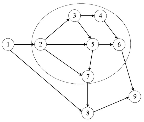
Figure 2.
A simple network with a charging cordon.
Table 2.
Travel demand information.
Table 3.
Link data.
Table 4.
Link–route incidence.
Table 5.
Internal routes which go through the charging cordon.
As can be seen in Table 5, there are 9 different routes going through the charging cordon, and travel distances inside the cordon range from 9 to 15. Similar to [19], it is assumed that the nonlinear distance-based toll is piecewise-linearly approximated by six intervals, which can be uniquely determined by seven vertexes. The length for each interval is one. Other parameters used are summarized as follows:
- planning period: 90 days;
- : 0.4, : 0.5, : 0.6, : 0.5, : 1.0;
- upper bound of the toll: 1;
- lower bound of the toll: 5;
- predetermined target of the average ETTC: 280000;
- number of populations per generation in the WOA: 50;
- maximum iteration in the WOA: 100.
Figure 3 shows the results of the optimal distance-based toll rate in this numerical experiment. As we can see, the optimal distance-based toll rate is indeed a nonlinear function with respect to travel distances. However, the optimal toll rate is different to the one obtained in [19]. The reasons are threefold: (1) The input demands are different between this study and [19]; (2) the DTD dynamics model in this paper takes into consideration the information broadcasting process (see Equation (6)), while the one in [19] does not consider this process; (3) the optimization objectives are different since this study aims to minimize variance over different days, while the study in [19] aims to minimize the maximal regret over different days.
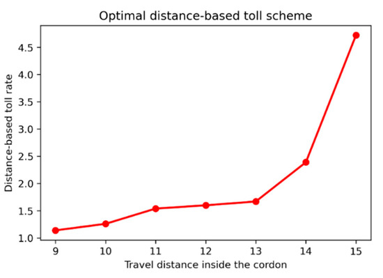
Figure 3.
Optimal distance-based toll scheme.
To validate the convergence of the proposed DTD dynamics model, Figure 4 shows the evolutionary processes of the flow and cost over the planning period. It is clear that the simple network can reach a steady state within 18 days. When increasing the network size, the number of days to reach a steady state may be much larger. Figure 5 shows the flow and cost evolution processes when an optimal toll is levied in the cordon. Comparing it with Figure 4, we can see that levying the congestion toll does not increase the convergence speed in this network with the corresponding parameters set in this experiment, and this is because the objective in the optimization model is to reduce risk and increase reward, rather than increasing the convergence speed. Figure 6 describes the expected total travel cost for each day. The ETTC keeps steady after 18 days since the system reaches the steady state, while it is fluctuant during the first 18 days.
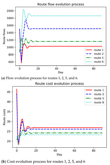
Figure 4.
Flow and cost evolution process when there is no toll charged in the cordon.
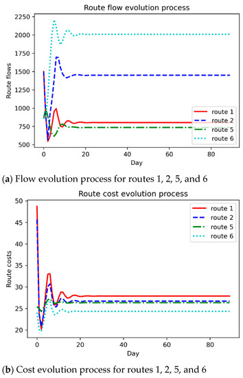
Figure 5.
Flow and cost evolution process when there the toll is levied in the cordon.
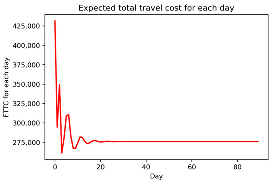
Figure 6.
Expected total travel cost for each day over the whole planning period.
6. Conclusions
This paper solves the optimal congestion pricing problem with DTD dynamics through the mean–variance optimization approach. Under the circumstance that traffic flows evolve from day to day and the system might be in a non-equilibrium state during a certain period of days after implementing a new congestion toll scheme, it is questionable to use an equilibrium-based index under a steady state as the objective to measure the performance of a congestion toll scheme. Consequently, a mean–variance-based toll scheme which takes into consideration the evolutionary flow dynamics from day to day is proposed to robustly optimize network system performance over the whole planning period. In the mean–variance-based optimization model, travelers aim to minimize the variance of ETTCs on different days to reduce risk the daily trips from day to day, while the mean of ETTCs over the whole planning period is restricted to being no larger than a predetermined target value set by the authorities. The proposed mean–variance-based DTD-DCP problem is solved by a metaheuristic approach based on the whale optimization algorithm, and the results from a numerical study validate the effectiveness of the proposed model and solution algorithm. As for future research, some extensions are recommended to further improve congestion pricing with DTD dynamics. On the one hand, identifying how to design an exact solution algorithm, rather than a metaheuristic method, is still a challenge for the DTD-DCP problem. On the other hand, it is still unclear how the DTD dynamics model influences the optimal toll rate in the DCP problem. More studies should be conducted to investigate these issues in future.
Author Contributions
Conceptualization, Q.C.; methodology, Q.C. and H.Z.; software, Q.C.; validation, Q.C., and H.Z.; formal analysis, Q.C. and H.Z.; writing—original draft preparation, Q.C.; writing—review and editing, Z.L. and J.C.; visualization, Q.C.; supervision, J.C. and Z.L. All authors have read and agreed to the published version of the manuscript.
Funding
This study is supported by the Key Projects (No. 51638004) of the National Natural Science Foundation of China and the Scientific Research Foundation of Graduate School of Southeast University (No. YBPY1885).
Conflicts of Interest
The authors declare no conflict of interest.
References
- Federal Highway Administration. FHWA Fiscal Year 2019 Budget; U.S. Department of Transportation: Washington, DC, USA, 2018.
- INRIX. 2018 Global Traffic Scorecard Report; INRIX Research: Altrincham, UK, 2019. [Google Scholar]
- Huang, D.; Gu, Y.; Wang, S.; Liu, Z.; Zhang, W. A two-phase optimization model for the demand-responsive customized bus network design. Transp. Res. Part C 2020, 111, 1–21. [Google Scholar] [CrossRef]
- Huang, D.; Chen, X.; Liu, Z.; Lyu, C.; Wang, S.; Chen, X. A static bike repositioning model in a hub-and-spoke network framework. Transp. Res. Part E 2020, 141, 102031. [Google Scholar] [CrossRef]
- Huang, D.; Xing, J.; Liu, Z.; An, Q. A multi-stage stochastic optimization approach to the stop-skipping and bus lane reservation schemes. Transp. A 2020, 1–33. [Google Scholar]
- Ma, J.; Xu, M.; Meng, Q.; Cheng, L. Ridesharing user equilibrium problem under OD-based surge pricing strategy. Transp. Res. Part B 2020, 134, 1–24. [Google Scholar] [CrossRef]
- Beijing Transport Institute. 2019 Beijing Transport Annual Report; Beijing Transport Institute: Beijing, China, 2019. [Google Scholar]
- Braess, D. Über ein Paradoxon aus der Verkehrsplanung. Unternehmensforschung 1968, 12, 258–268. [Google Scholar] [CrossRef]
- Braess, D.; Nagurney, A.; Wakolbinger, T. On a paradox of traffic planning. Transp. Sci. 2005, 39, 446–450. [Google Scholar] [CrossRef]
- Olszewski, P.; Xie, L. Modelling the effects of road pricing on traffic in Singapore. Transp. Res. Part A 2005, 39, 755–772. [Google Scholar] [CrossRef]
- Tang, C.K. The cost of traffic: Evidence from the London congestion charge. J. Urban Econ. 2021, 121, 103302. [Google Scholar] [CrossRef]
- Percoco, M. Is road pricing effective in abating pollution? Evidence from Milan. Transp. Res. Part D 2013, 25, 112–118. [Google Scholar] [CrossRef]
- Borjesson, M.; Eliasson, J.; Hugosson, M.B.; Brundell-Freij, K. The Stockholm congestion charges—5 years on effects, acceptability and lessons learnt. Transp. Policy 2012, 20, 1–12. [Google Scholar] [CrossRef]
- Yang, H.; Huang, H.-J. Mathematical and Economic Theory of Road Pricing; Elsevier Ltd.: Amsterdam, The Netherlands, 2005. [Google Scholar]
- de Palma, A.; Lindsey, R. Traffic congestion pricing methodologies and technologies. Transp. Res. Part C 2011, 19, 1377–1399. [Google Scholar] [CrossRef]
- Cheng, Q.; Liu, Z.; Liu, F.; Jia, R. Urban dynamic congestion pricing: An overview and emerging research needs. Int. J. Urban Sci. 2017, 21, 3–18. [Google Scholar] [CrossRef]
- Gu, Z.; Liu, Z.; Cheng, Q.; Saberi, M. Congestion pricing practices and public acceptance: A review of evidence. Case Stud. Transp. Policy 2018, 6, 94–101. [Google Scholar] [CrossRef]
- Selmoune, A.; Cheng, Q.; Wang, L.; Liu, Z. Influencing factors in congestion pricing acceptability: A literature review. J. Adv. Transp. 2020, 2020, 4242964. [Google Scholar] [CrossRef]
- Liu, Z.; Wang, S.; Zhou, B.; Cheng, Q. Robust optimization of distance-based tolls in a network considering stochastic day to day dynamics. Transp. Res. Part C 2017, 79, 58–72. [Google Scholar] [CrossRef]
- Wie, B.; Tobin, R. Dynamic congestion pricing models for general traffic networks. Transp. Res. Part B 1998, 32, 313–327. [Google Scholar] [CrossRef]
- Sandholm, W.H. Evolutionary implementation and congestion pricing. Rev. Econ. Stud. 2002, 69, 667–689. [Google Scholar] [CrossRef]
- Friesz, T.L.; Bernstein, D.; Kydes, N. Dynamic congestion pricing in disequilibrium. Netw. Spat. Econ. 2004, 4, 181–202. [Google Scholar] [CrossRef]
- Yang, F.; Szeto, W. Day-to-day dynamic congestion pricing policies towards system optimal. In Proceedings of the First International Symposium on Dynamic Traffic Assignment, Leeds, UK, 21 June 2006; pp. 266–275. [Google Scholar]
- Yang, F.; Yin, Y.; Lu, J. Steepest descent day-to-day dynamic toll. Transp. Res. Rec. 2007, 2039, 83–90. [Google Scholar] [CrossRef]
- Yang, F. Day-to-day dynamic optimal tolls with elastic demand. In Proceedings of the 87th Transportation Research Board Annual Meeting, Washington, DC, USA, 13 January 2008. [Google Scholar]
- Guo, X. Toll sequence operation to realize target flow pattern under bounded rationality. Transp. Res. Part B 2013, 56, 203–216. [Google Scholar] [CrossRef]
- Wang, Y.; Liu, H.; Han, K.; Friesz, T.L.; Yao, T. Day-to-day congestion pricing and network resilience. Transp. A 2015, 11, 873–895. [Google Scholar] [CrossRef]
- Ma, X.; Xu, W.; Chen, C. A day-to-day dynamic evolution model and pricing scheme with bi-objective user equilibrium. Transp. B 2021, 9, 283–302. [Google Scholar]
- Guo, R.-Y.; Yang, H.; Huang, H.-J.; Tan, Z. Day-to-day flow dynamics and congestion control. Transp. Sci. 2016, 50, 982–997. [Google Scholar] [CrossRef]
- Ye, H.; Yang, H.; Tan, Z. Learning marginal-cost pricing via a trial-and-error procedure with day-to-day flow dynamics. Transp. Res. Part B 2015, 81, 794–807. [Google Scholar] [CrossRef]
- Xu, M.; Meng, Q.; Huang, Z. Global convergence of the trial-and-error method for the traffic-restraint congestion-pricing scheme with day-to-day flow dynamics. Transp. Res. Part C 2016, 69, 276–290. [Google Scholar] [CrossRef]
- Chen, X.; Wang, Y.; Zhang, Y. A trial-and-error toll design method for traffic congestion mitigation on large river-crossing channels in a megacity. Sustainability 2021, 13, 2749. [Google Scholar] [CrossRef]
- Tan, Z.; Yang, H.; Guo, R.Y. Dynamic congestion pricing with day-to-day flow evolution and user heterogeneity. Transp. Res. Part C 2015, 61, 87–105. [Google Scholar] [CrossRef]
- Wang, X.; Ye, H.; Yang, H. Decentralizing Pareto-efficient network flow/speed patterns with hybrid schemes of speed limit and road pricing. Transp. Res. Part E Logist. Transp. Rev. 2015, 83, 51–64. [Google Scholar] [CrossRef]
- Gehlot, H.; Honnappa, H.; Ukkusuri, S. V An optimal control approach to day-to-day congestion pricing for stochastic transportation networks. Comput. Oper. Res. 2020, 119, 104929. [Google Scholar] [CrossRef]
- Li, D.; Ng, W.-L. Optimal dynamic portfolio selection: Multiperiod mean-variance formulation. Math. Financ. 2000, 10, 387–406. [Google Scholar] [CrossRef]
- Björk, T.; Murgoci, A.; Zhou, X.Y. Mean-variance portfolio optimization with state-dependent risk aversion. Math. Financ. 2014, 24, 1–24. [Google Scholar] [CrossRef]
- Mirjalili, S.; Lewis, A. The whale optimization algorithm. Adv. Eng. Softw. 2016, 95, 51–67. [Google Scholar] [CrossRef]
- Meng, Q.; Liu, Z.; Wang, S. Optimal distance tolls under congestion pricing and continuously distributed value of time. Transp. Res. Part E 2012, 48, 937–957. [Google Scholar] [CrossRef]
- Cheng, Q.; Liu, Z.; Szeto, W.Y. A cell-based dynamic congestion pricing scheme considering travel distance and time delay. Transp. B 2019, 7, 1286–1304. [Google Scholar] [CrossRef]
- Liu, Z.; Wang, S.; Meng, Q. Optimal joint distance and time toll for cordon-based congestion pricing. Transp. Res. Part B 2014, 69, 81–97. [Google Scholar] [CrossRef]
- LTA. Land Transport Master Plan 2013; Singapore Land Transport Authority: Singapore, 2013.
- Ye, H.; Xiao, F.; Yang, H. Day-to-day dynamics with advanced traveler information. Transp. Res. Part B 2021, 144, 23–44. [Google Scholar] [CrossRef]
- Cantarella, G.E.; Cascetta, E. Dynamic processes and equilibrium in transportation networks: Towards a unifying theory. Transp. Sci. 1995, 29, 305–329. [Google Scholar] [CrossRef]
- Cheng, Q.; Wang, S.; Liu, Z.; Yuan, Y. Surrogate-based simulation optimization approach for day-to-day dynamics model calibration with real data. Transp. Res. Part C 2019, 105, 422–438. [Google Scholar] [CrossRef]
- Elton, E.J.; Gruber, M.J. Modern portfolio theory, 1950 to date. J. Bank. Financ. 1997, 21, 1743–1759. [Google Scholar] [CrossRef]
- Gharehchopogh, F.S.; Gholizadeh, H. A comprehensive survey: Whale Optimization Algorithm and its applications. Swarm Evol. Comput. 2019, 48, 1–24. [Google Scholar] [CrossRef]
- Sony, B.; Chakravarti, A.; Reddy, M.M. Traffic congestion detection using whale optimization algorithm and multi-support vector machine. Int. J. Recent Technol. Eng. 2019, 7, 589–593. [Google Scholar]
- Zhang, H.; Tang, L.; Yang, C.; Lan, S. Locating electric vehicle charging stations with service capacity using the improved whale optimization algorithm. Adv. Eng. Inform. 2019, 41, 100901. [Google Scholar] [CrossRef]


Publisher’s Note: MDPI stays neutral with regard to jurisdictional claims in published maps and institutional affiliations. |
© 2021 by the authors. Licensee MDPI, Basel, Switzerland. This article is an open access article distributed under the terms and conditions of the Creative Commons Attribution (CC BY) license (https://creativecommons.org/licenses/by/4.0/).