Carbon Price Forecasting Based on Improved CEEMDAN and Extreme Learning Machine Optimized by Sparrow Search Algorithm

Abstract

Effective carbon pricing policies have become an effective tool for many countries to encourage emission reduction. An accurate carbon price prediction model is helpful for the implementation of energy conservation and emission reduction policies and the decision-making of governments and investors. However, it is difficult for a single prediction model to achieve high prediction accuracy because of the high complexity of the carbon price series. Many studies have proved the nonlinear characteristics of carbon trading prices, but there are very few studies on the chaotic nature of carbon price series. As a consequence, this paper proposes an innovative hybrid model for carbon price prediction. A decomposition-reconstruction-prediction-integration scheme is designed to predict carbon prices. Firstly, several intrinsic mode functions (IMFs) and one residue were obtained from the raw data decomposed by ICEEMDAN. Next, the decomposed subsection is reconstructed into a new sequence according to the calculation results by the Lempel-Ziv complexity algorithm. Then, considering the chaotic characteristics of sequence, the input variables of the models are determined through the phase space reconstruction (PSR) algorithm combined with the partial autocorrelation function (PACF). Finally, the Sparrow search algorithm (SSA) is introduced to optimize the extreme learning machine (ELM) model, which is applied in the carbon price prediction for the purpose of verifying the validity of the proposed combination model, which is applied to the pilots of Hubei, Beijing, and Guangdong. The empirical results show that the combination model outperformed the 13 other models in predicting accuracy, speed, and stability. The decomposition-reconstruction-prediction-integration strategy is a method for predicting the carbon price efficiently.

1. Introduction

The consequences of environmental climate change caused by the intensification of global energy consumption threaten the sustainable development of mankind. The “Kyoto Protocol” officially came into effect, which means that countries have begun to curb global warming by controlling greenhouse gas emissions. The EU took the lead in establishing a carbon emissions trading market. The carbon market has become an effective mechanism for mitigating climate change and has been highly valued by governments and organizations around the world [1]. As the largest developing country and emitter of greenhouse gas emissions, China has been working to reduce greenhouse gas emissions. China has established eight carbon market trading points since 2013 and hopes to build a unified national carbon emissions trading market [2]. In the carbon market, carbon price is the main factor. Changes in carbon prices have an important impact on industry, energy, agricultural development, and stock investment [3,4,5]. Carbon price forecasting is of great significance in carbon trading, which is conducive to government decision-making and reducing investor risks [6], and is conducive to a better establishment of a stable carbon pricing mechanism [7].

The Chinese government proposes to achieve a carbon peak in 2030 and a goal of achieving carbon neutrality by 2060. To this end, China is committed to the construction of a unified national carbon market [8]. Accurate carbon trading price forecasts help to unify the implementation of carbon market policies. Therefore, since the establishment of China’s carbon market trading pilot, the study of carbon prices has received extensive attention from scholars. Many studies have proved that carbon trading prices can be studied as a time series [9], and due to the influence of economic, policy, weather, and other factors, carbon prices show nonlinear and non-stationary characteristics [10]. In previous research, traditional econometric models, such as the generalized autoregressive conditional heteroscedasticity model (GARCH) and autoregressive moving average model (ARMA), among others, were applied in the field of carbon price prediction. However, these studies are based on the premise of stable data and linear assumptions and do not consider the nonlinear issue of carbon prices. For this reason, the introduction of intelligent algorithms such as Back Propagation Neuron (BP), Radial Basis Function (RBF), Least Squares Support Vector Machine (LSSVM), and Extreme Learning Machine (ELM) has solved this problem [11]. However, the existing prediction models only consider the nonlinearity and non-stationarity of the carbon price series. The selection of input characteristic variables is often limited to repeated experiments or linear regression. The chaotic characteristics of the carbon price series are not sufficiently studied [12]. Therefore, this article fully considers the chaotic characteristics of the carbon valence series. The phase space reconstruction and partial autocorrelation analysis are combined to determine the feature selection of the prediction model. Besides, it is difficult for a single forecasting model to achieve higher accuracy, so more and more researchers tend to combine forecasting models [13]. At the same time, to better solve the nonlinear and non-stationary problems of carbon price series, the combined model based on the decomposition-prediction-integration strategy has been widely used by scholars in carbon price forecasting [14]. This article continues this strategy and makes improvements on this basis.

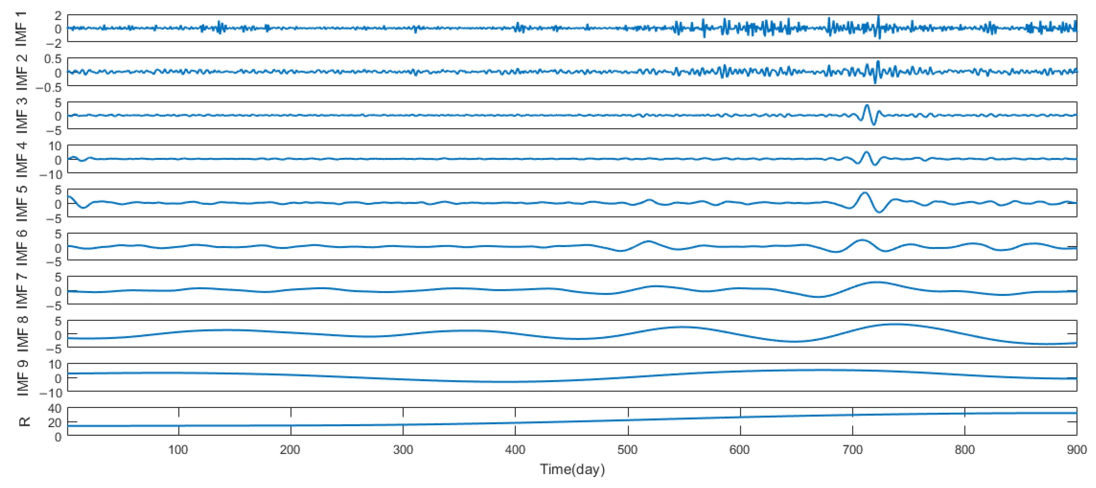
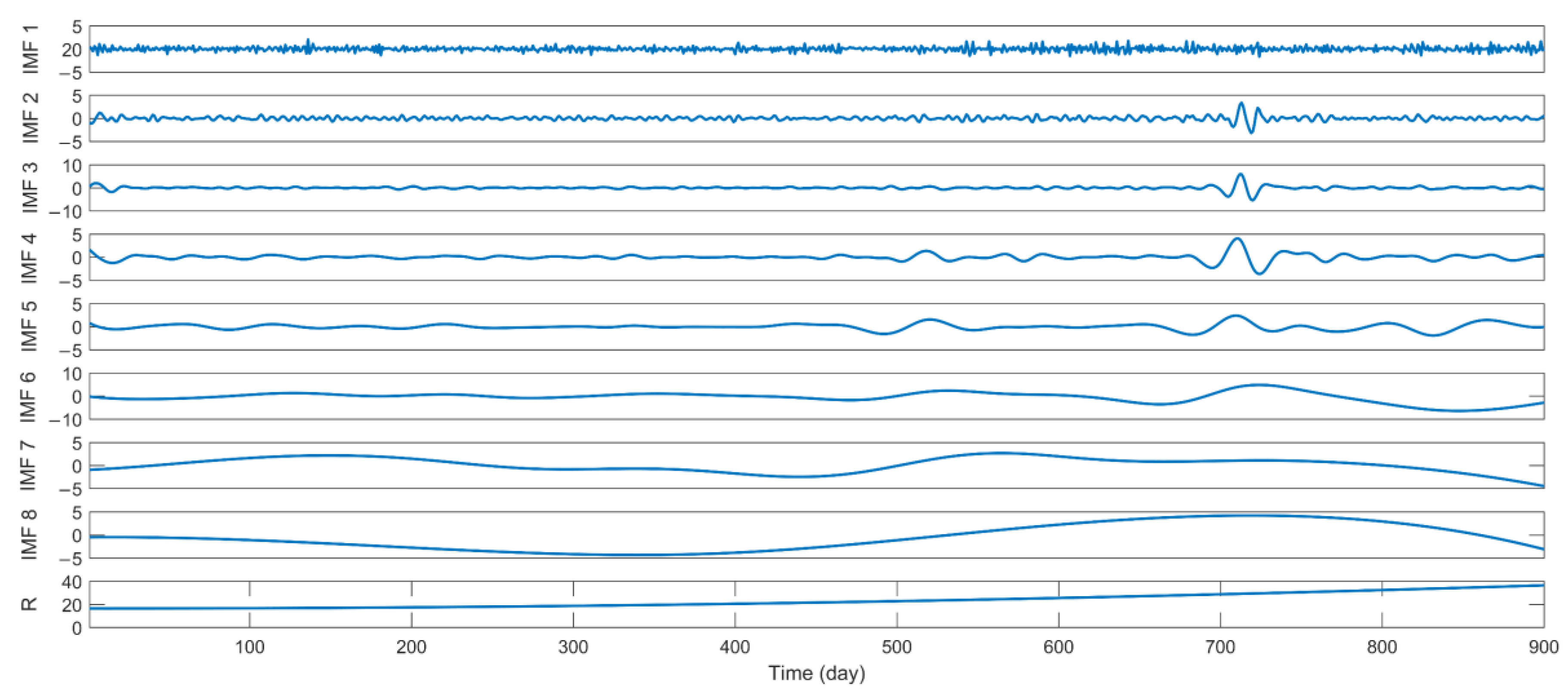
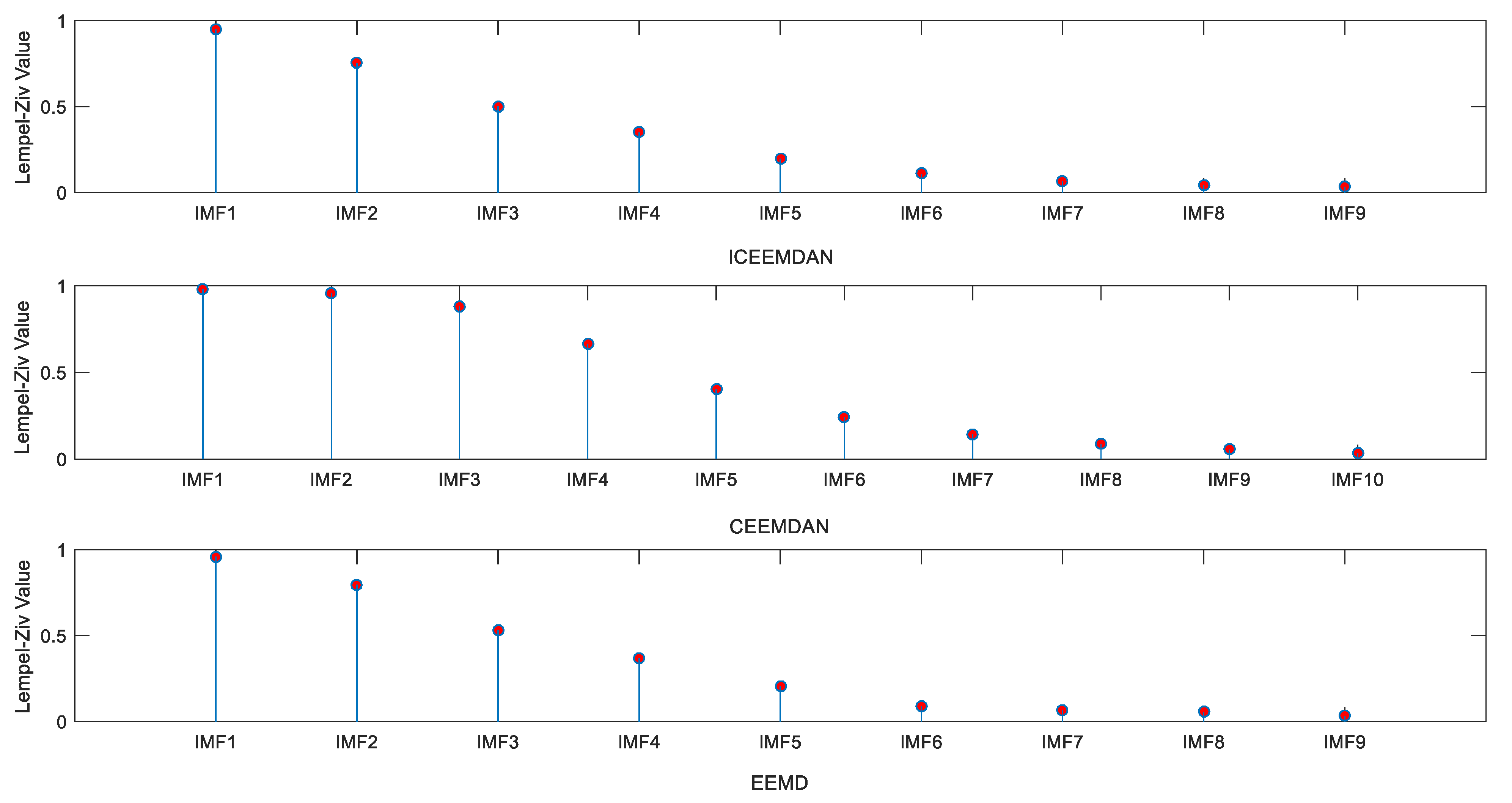
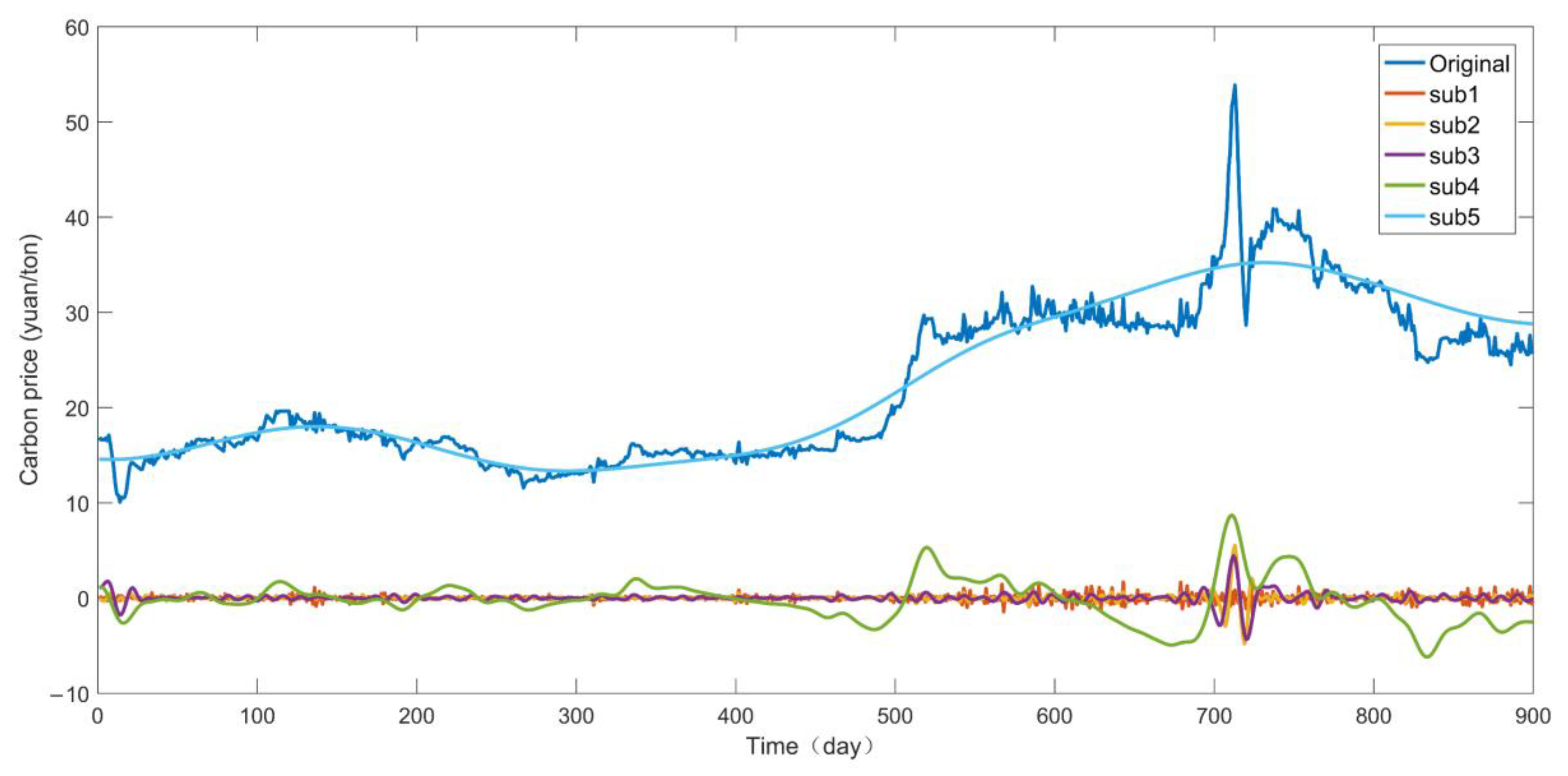
The purpose of this paper is to establish a new hybrid model to improve the accuracy of carbon price forecasts. The prediction model includes data pretreatment, feature selecting, intelligent optimization algorithm, and prognostication. The main details are as follows. Firstly, the improved CEEMDAN (ICEEMDAN) model with better performance is applied in the decomposition of the original sequence. Secondly, the Lempel–Ziv complex arithmetic was introduced to remodel the subsequence into a new subsequence (Subs). Then, the input parameters of each subsequence were confirmed by the phase space reconstruction (PSR) combine with partial autocorrelation function (PACF). At last, the carbon price sequence was predicted by the SSA-ELM model, and the final prediction result was obtained by integrating the prediction results of each subsequence. For the sake of validating the hybrid model, we applied the mixed model in Hubei, Guangdong, and Beijing carbon markets for testing.

The remainder of this article is organized as follows. The fundamental theory methods of the model and the construction of the ICEEMDAN-PSR-SSA-ELM model are described in Section 2. Section 3 presents the course of empirical analysis containing the raw data analysis and processing. Section 4 shows the carbon price prediction results and discussions. In the end, the conclusions based on experiments are given in Section 5.

2. Literature Review

At present, there is a large amount of research into carbon price prediction that works by establishing a prediction model. The predictive models can mainly be classified into two types: one is based on establishing a single model, and the other is based on establishing a combined model.

In previous research, the generalized autoregressive conditional heteroscedasticity model (GARCH), Kalman prediction model, autoregressive moving average model (ARMA), gray model, and other econometric models have been used in many forecasting fields [15]. Paolella and Taschini [16] analyzed the carbon price by GARCH, and found that the GARCH model with different distribution assumptions can provide accurate out-of-sample risk value prediction. Byun and Cho [17] applied different types of GARCH models to predict carbon futures in the aspect of volatility and proved that the GJR-GARCH model with normal distribution performs excellently in comparison to the k-nearest neighbor (K-NN) model and has the best prediction performance. Zhao et al. [18] researched the carbon price by applied the combination mixed data sampling (MIDAS) recursive model, and the prediction result fits the actual value. However, although these models based on stable data and linear assumptions can get good prediction results, the nonlinearity problem of carbon prices cannot be solved effectively [19].

Aiming at the problem of nonlinearity and non-stationarity of carbon price series, neural network models with better performance in dealing with nonlinear problems have been used for the research of carbon price prediction. Han et al. [11] verified that the combination-MIDAS-BP(Back Propagation Neuron NetWok) model is applicable to the price prediction of the Shenzhen carbon market in China. Tsai and Kuo [20] combined the prices of oil, natural gas, coal, etc. and predict European carbon prices with the Radial Basis Function (RBF) model. The study demonstrates that the RBF model is prior to BP in the prediction performance. Zhu [21] used empirical mode decomposition (EMD) to process the data in the first step and binding of genetic algorithm (GA) to the artificial neural network (ANN) to predict carbon prices. Research shows that the combined model is prior to a single Autoregressive Integrated Moving Average (ARIMA) and ANN model. Zhu and Wei [22] combined ARIMA with LSSVM to predict carbon prices; furthermore, they applied particle swarm optimization (PSO) to optimize the parameter of LSSVM and found that the accuracy of mixed-model exceeds that of the single model. Combining the literature, it can be seen that BP and RBF rely on data samples. When the data is insufficient, the fitness may be poor. LSSVM relies on the selection of kernel function and kernel parameters. Different choices may affect the prediction effect to varying degrees.

The Extreme Learning Machine (ELM) model converges faster with less artificial interference in contrast to the traditional neural network model. It has been widely employed in many fields of prediction. Zhang et al. [23] used the ELM to forecast the power load of Australia, and the results show that it is superior to the BP and RBF models. Li et al. [24] used the method of combining the ELM with partial least square regression (PLS) for load prediction, and that the ELM has higher forecasting performance was verified experimentally. The ELM model was applied to stock price prediction, which proved that the prediction accuracy of the ELM model outperformed the traditional neural network model [25,26]. From the above, it can be seen that the ELM has been used in various applications widely and effectively in varied domains of forecasting. However, the randomly assigned input weight matrix and hidden layer deviation will affect the generalization ability of ELM. Therefore, it is very necessary to use an optimization algorithm to obtain the optimal weight of the input layer and the optimal deviation of the hidden layer. Sun et al. [17] applied the particle swarm optimization the extreme value learning machine for carbon emission prediction research. Zhou et al. [27] used Grey Wolf Optimizer (GWO) binding to the ELM model to predict carbon prices, which indicated that the predictive precision of the optimized ELM model outperformed the single ELM. Sun and Zhang [15] applied the extreme learning machine optimized by the adaptive whale optimization algorithm to carbon price prediction, and the results verified that the optimized ELM performance is more accurate than before the optimization. In summary, a suitable optimization algorithm can improve the performance of ELM. Sparrow Search Algorithm (SSA), a swarm intelligence optimization algorithm, was first put forward in 2020 [28]. The SSA performed better in competition with the other most advanced algorithms (such as the GWO, PSO, and so on) from the viewpoint of search accuracy, convergent velocity, and stability. Therefore, this paper introduces SSA to ascertain the input weights and hidden layer thresholds of ELM, which could maximize the capabilities of global and local searches to solve the unsteadiness of ELM and other problems.

In view of the complexity and non-stationarity of carbon prices, it is difficult to obtain accurate results only with the optimized ELM prediction model [29]. Therefore, to better predict carbon prices, the original sequence of carbon prices needs to be further decomposed. Empirical mode decomposition (EMD) is a familiar decomposing method that has attracted the attention of researchers. Using the EMD to pre-process carbon price series can better analyze the internal characteristics of the series. Compared with a single non-decomposing model, the hybrid EMD can more effectively improve the prediction accuracy [19]. However, EMD has the problem of modal mixing. To tackle this problem, Wu and Huang [30] put forward the Ensemble Empirical Mode Decomposition (EEMD) model. Sun and Xu [31] applied the EEMD to carbon price decomposition, and the experimental results prove that the performance of EEMD is better than that of EMD. However, while solving the inherent modal mixing problem of EMD, EEMD brings new modal mixing problems. To this end, for solving the problems of EEMD, the complete ensemble empirical mode decomposition with adaptive noise (CEEMDAN) was proposed [32]. Colominas et al. [33] proposed Improved CEEMDAN (ICEEMDAN) on the basis of previous research, and this method further resolves the problems of the existence of residual noise in the modes and false modes in the CEEMDAN method. The ICEEMDAN method has been applied to the research of crude oil prices and electricity load forecasting, which verified the superiority of ICEEMDAN method in processing complex data. However, the application of the ICEEMDAN method to carbon price research has not yet been attempted. Therefore, this article innovatively applies the ICEEMDAN method to carbon price prediction. The experimental results verify its superior performance.

-

In an effort to contribute to the literature, we have also selected the real carbon price data from Hubei, Guangdong, and Beijing carbon trading pilots for example analysis. Firstly, several IMFs and one residue were obtained from the raw data decomposed by ICEEMDAN. Next, the decomposed subsection was reconstructed into a new sequence according to the calculation results of the Lempel–Ziv complexity algorithm. Then, considering the chaotic characteristics of sequence, the input variables of the models were determined through the PSR algorithm combined with PACF. Finally, the SSA was introduced to optimize the ELM model, which is applied in the carbon price prediction. This article innovatively applies the ICEEMDAN to carbon price decomposition, and the experimental results verify its superior performance.

-

The ICEEMDAN can consider the chaotic characteristics of carbon prices and combine phase space reconstruction with partial autocorrelation analysis to select the input feature variables of the predictive model.

-

The ELM optimized by the SSA algorithm has higher prediction accuracy. The established hybrid model has higher stability and robustness and is more suitable for carbon price prediction research.

3. Methodology

3.1. ICEEMDAN

The ICEEMDAN algorithm is a further improvement based on the EEMD and CEEMDAN algorithms and has wide applicability in numerous fields. Experiments show that ICEEMDAN solves the possible residual noise in the EEMD algorithm and the possible false modes problem in the CEEMDAN algorithm, effectively improving the noise reduction effect [34,35,36]. The specific steps of the ICEEMDAN algorithm are as follows:

Let $H(·)$ be the operator which produces the local mean of the signal that is applied to. $E_k(·)$ as the $k$th modal component obtained by using the EMD method to decompose, and let ${\xi }^i$ be a white Gaussian noise which can achieve zero mean and unit variance.

The $k$th modaxl component produced by ICEEMDAN is denoted as $\overrightarrow{{IMF}_k}$. On the basis of the EMD algorithm flow, the ICEEMDAN algorithm steps are as follows:

Step 1: The first residue can be gained by EMD calculation; the local means $x^i\left(t\right)=x\left(t\right)+{\epsilon }_0{E}_1\left({\xi }^i\left(t\right)\right)$:

$$r_1=\langle H(x^i(t))\rangle$$

(1)

Equation (1) is the first residue, where ${\epsilon }_0={\delta }_{0}std\left(x\right)/std\left(E_1\left({\xi }^i\left(t\right)\right)\right)$ represents the level of noise.

Step 2: In the first phase $(k=1)$, the first mode is calculated from:

$$\overrightarrow{IM{F}_1}(t)=x(t)-r_1(t)$$

(2)

Step 3: Estimate the second residual as the average of the local mean of $r_1\left(t\right)+{\epsilon }_1{E}_2\left[{\xi }^i\left(t\right)\right]$ and define the second mode:

$$\overrightarrow{IM{F}_2}=r_1(t)-r_2(t)=r_1(t)-\langle H(r_1(t)-{\omega }_1{E}_2({\xi }^i(t)))\rangle$$

(3)

Step 4: For the remaining stage, calculate the $k$th residual:

$$r_k(t)=\langle H(r_{K-1}(t)-{\omega }_{K-1}{E}_k({\xi }^i(t)))\rangle$$

(4)

Calculate the $k$th mode:

$$\overrightarrow{IM{F}_k}(t)=r_{k-1}(t)-r_k(t)$$

(5)

where $k=3,\dots ,K$.

Step 5: Go to step 4 for nex $k$.

3.2. PSR

Takens [37] first proposed phase space reconstruction (PSR) theory in 1981. PSR is often used to study chaotic time series and is considered an effective method to reconstruct the phase space of chaotic series [38]. PSR mainly delays the coordinate state of a given sequence and expands it to a high-dimensional space to reveal its hidden information [39]. Therefore, PSR can be applied to analyze the various subsequences of carbon prices to display hidden information, which determines input variables more accurately and increases the accuracy of the model of the forecast. The principle of PSR is as follows:

Let $x\left(t\right)=\left\{x_1,x_2,\dots ,x_N\right\}$ be a chaotic time series, denote by $\tau$ and $m$ the delay time and the embedding dimension individually; the reconstructed phase space is:

$$X(t)=\left[\begin{array}{cccc}{x}_{(1)}& x_{(1+\tau )}& \cdots & x_{(1+(m-1)\tau )}\\ x_{(2)}& x_{(2+\tau )}& \cdots & x_{(2+(m-1)\tau )}\\ ⋮& ⋮& ⋮& ⋮\\ x_{(M)}& x_{(M+\tau )}& \cdots & x_{(M+(m-1)\tau )}\end{array}\right]$$

(6)

Equation (6) represents the reconstructed phase space, the $t$ is phase point in the phase space: $t=1,2,\dots ,M$, and $M=n-\left(m-1\right)\tau$.

The $\tau$ and $m$ are the key to the PSR. In this paper, the delay time $\tau$ was settled by using the mutual information method, which is easy to calculate and suitable for nonlinear problems [40], and the $m$ is determined by applying the CAO method [41]. The Maximum Lyapunov index (MLYE) is often used to judge the chaos of the time series. When the MLYE is greater than zero, it indicates that the time series is chaotic. This article uses the “Wolf” method to determine the MLYE [42,43].

3.3. SSA

The sparrow search algorithm (SSA) is a new type of swarm intelligence optimization algorithm jointly proposed by Xue and Shen in 2020 [28]. There are two types of sparrow populations: explorers and followers. Explorers actively seek food sources, and followers get food from explorers. In addition, there are predators looting food. The specific implementation procedure of the SSA is as follows.

The location update formula of the explorer is as follows:

$$X_{i,j}^{t+1}=\{\begin{array}{cc}{X}_{i,j}^t\cdot \exp \left(\frac{-i}{\alpha \cdot ite{r}_{\max }}\right)\hfill & R_2<ST\hfill \\ X_{i,j}^t+Q\cdot L\hfill & R_2\ge ST\hfill \end{array}$$

(7)

In Equation (7), where $j=1,2,\dots ,d$, $t$ represents the number of iterations, when the $t$th iteration, $X_{i,j}^{t+1}$ denotes the value of the $i$th sparrow in the $j$th dimension. ${iter}_{\max }$ denotes the maximum number of iterations. $\alpha \in 0,1$ is a general random number. $R_2\in \left[0,1\right]$ and $ST\in \left[0.5,1\right]$ represent the precaution value and security threshold individully. $Q$ is a stochastic number that submits to a gaussian distribution, and $L$ is a matrix $(1\times d)$ with all elements as 1.

This means that there is no predator when $R_2<ST$, and the explorer will unfold a large-scale search pattern; contrarily, the predator is found when $R_2\ge ST$, and all sparrows should migrate to other safety regions quickly.

The follower’s location update formula is as follows:

$$x_{i,j}^{t+1}=\{\begin{array}{cc}Q\cdot \exp \left(\frac{X_w^t-X_{i,j}^t}{i^2}\right)& i>n/2\hfill \\ X_P^{t+1}+\left|X_{i,j}^t-X_P^{t+1}\right|\cdot A^{+}\cdot L& otherwise\hfill \end{array}$$

(8)

In Equation (8), where $X_P$ represents the explorer’s current optimal location, $X_W$ represents the present global worst position. $A$ is a matrix $(1\times d)$ with each element apportioned a value of 1 or −1 stochastically, and $A^{+}=A^T(A{A}^T{)}^{-1}$. This means the $i$th joiner with the worse adaptation degree has not received food and needs to go to other areas for food when $i<n/2$.

Assuming that the dangerous sparrows occupy 10% to 20% of the total, and to stochastically generate the original locations of these sparrows [28], the global optimal location formula is established as:

$$X_{i,j}^{t+1}=\{\begin{array}{cc}{X}_b^t+\beta \cdot \left|X_{i,j}^t-X_b^t\right|\hfill & f_i>f_g\hfill \\ X_{i,j}^t+K\cdot (\frac{\left|X_{i,j}^t-X_w^t\right|}{(f_i-f_w)+\lambda })\hfill & f_i>f_g\hfill \end{array}$$

(9)

In Equation (9), where $k\in \left[-1,1\right]$ represents a stochastic number, $X_b$ is the current optimal location of global, and $\beta$ is the step-length control parameter, which is a stochastic number that obeys a normal distribution (Mean value = 0, Variance = 1). Where $f_i$ denotes the fitness value of the current individual. $f_g$ and $f_w$ denote the present global best and worst fitness value separately. $\lambda$ represents the minimal constant for avoiding the denominator equals to 0.

3.4. ELM

Extreme Learning Machine (ELM) was constructed by Huang et al., which is a feedforward neural network with only one hidden layer [44]. The generalization performance of ELM outperformed traditional neural network models [45]. When we want to get the unique optimal solution in the process of training, we only need to set the neuron number in the hidden layer without adjusting its parameters [46].

What needs attention is the following: although it expedites the learning speed greatly to set the input weights and hidden layer deviations randomly, unsatisfactory selection of weights and thresholds may cause ELM performance degradation, and the result may be unstable [47]. This paper applies the sparrow optimization algorithm to adjust the weight biases of the input and hidden layer of the ELM model.

3.5. The Proposed Model

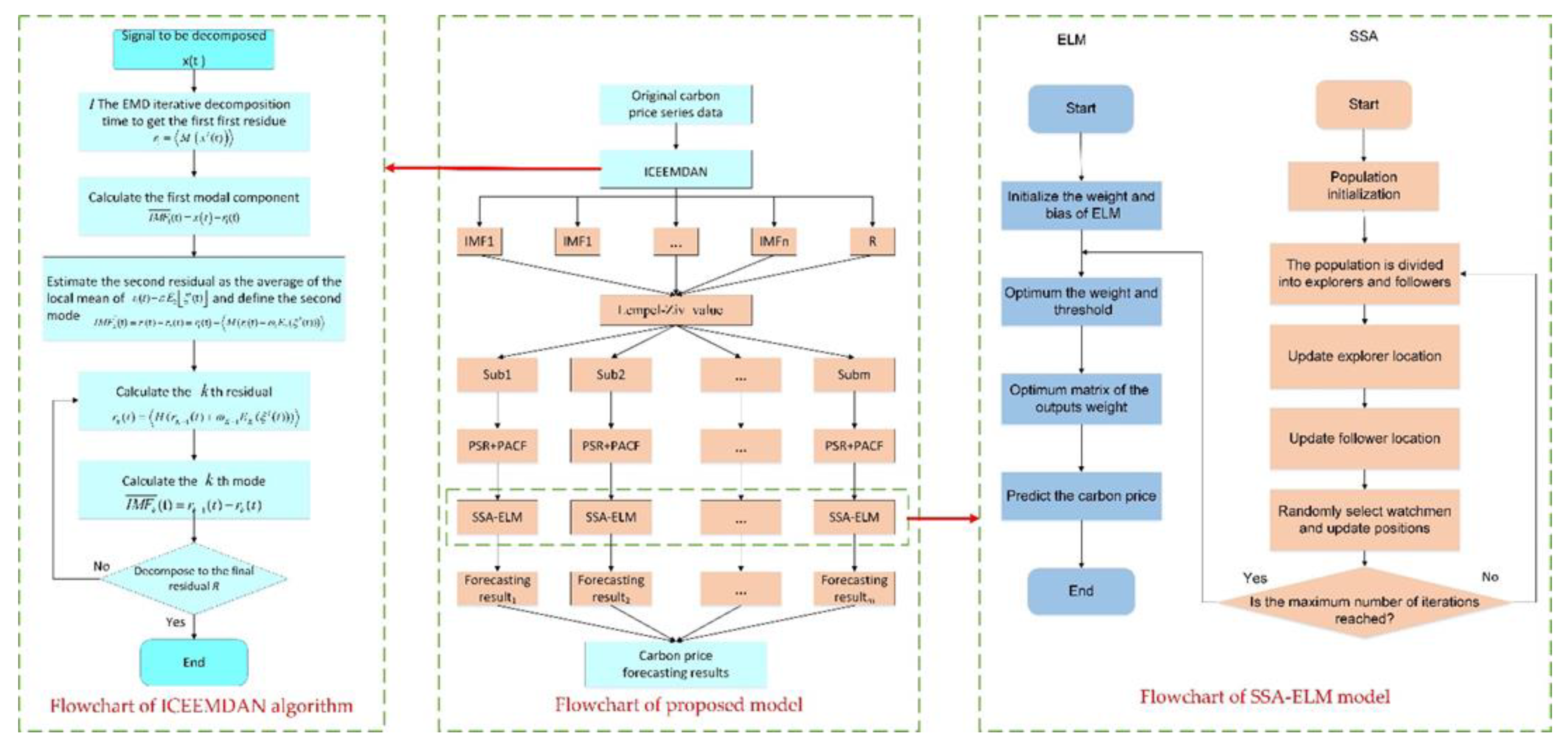
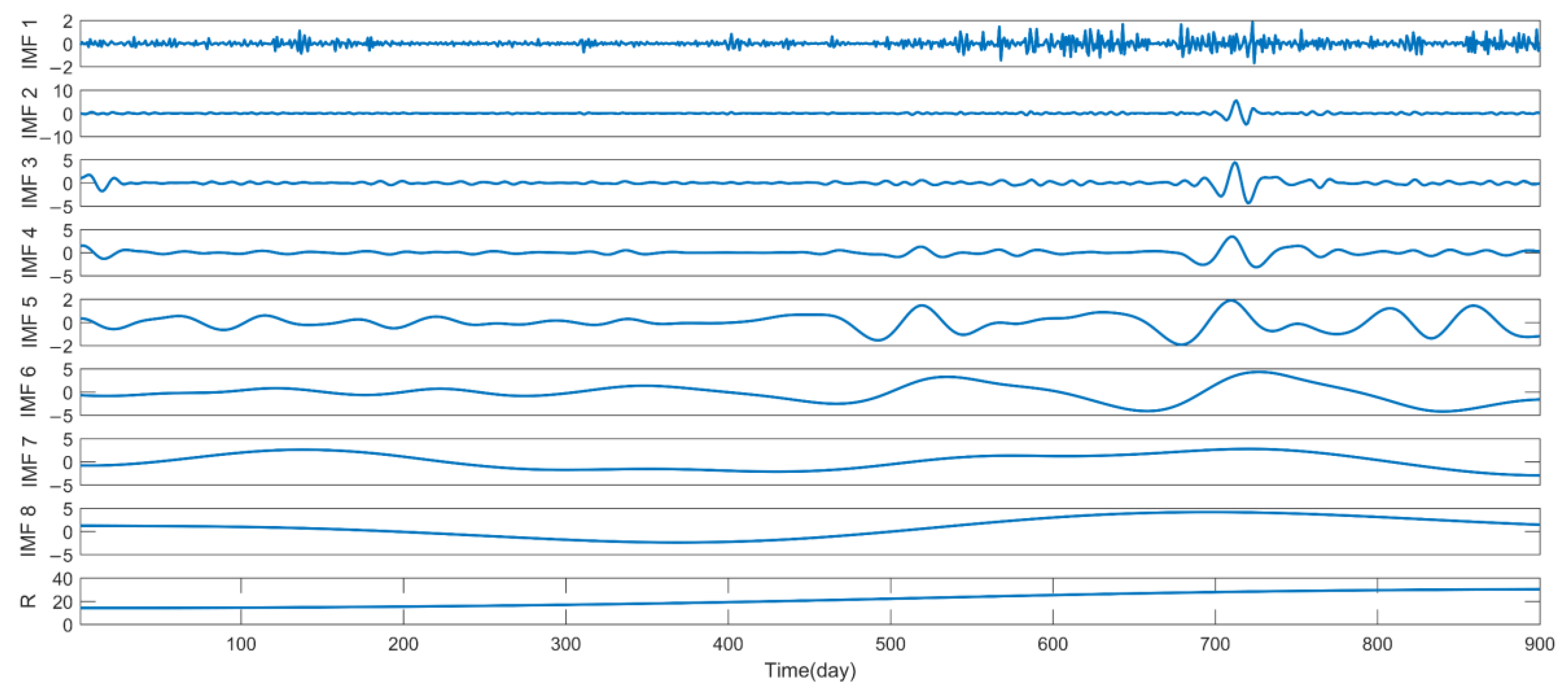
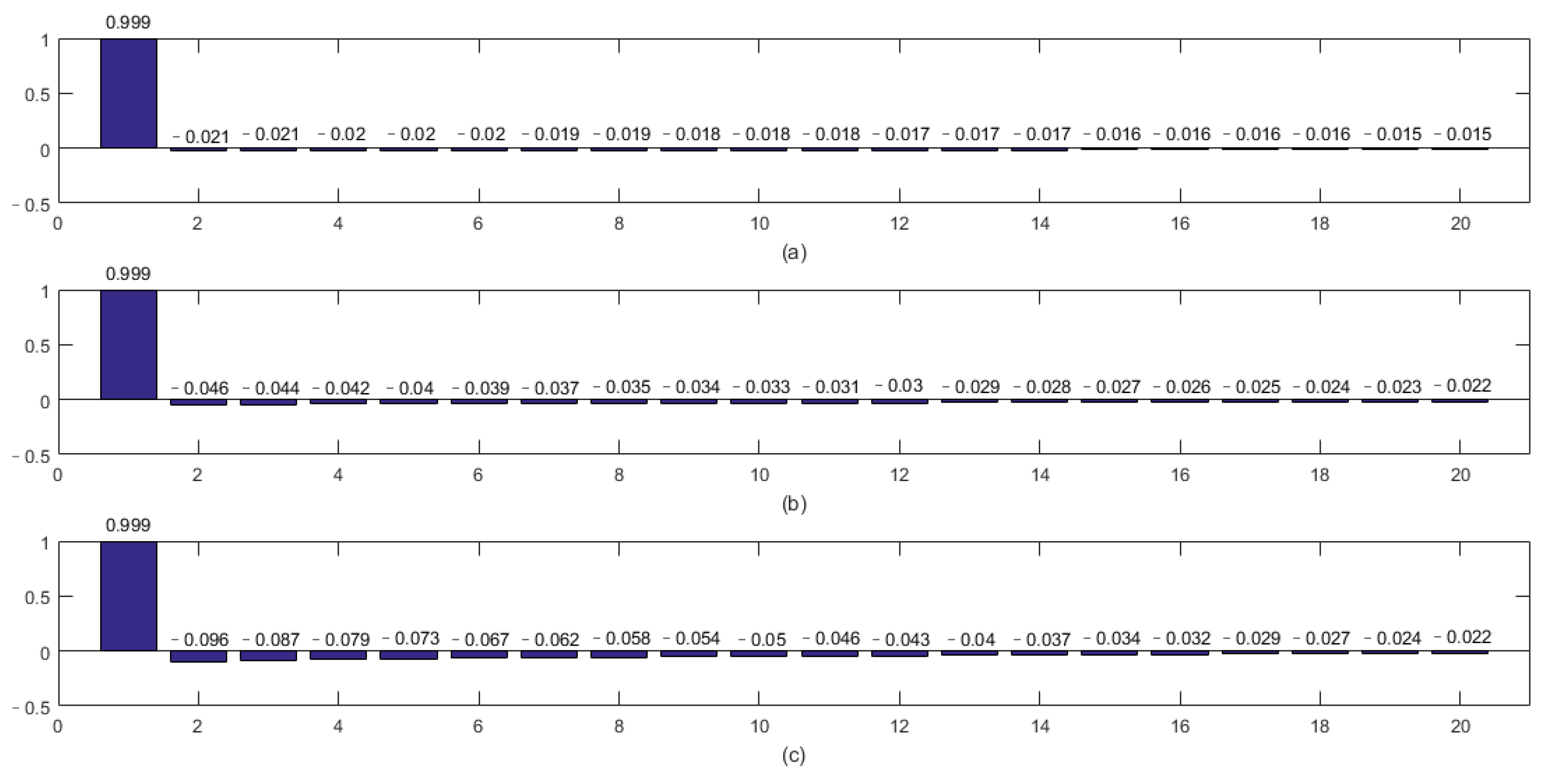
The flowchart of the ICEEMDAN-PSR-SSA-ELM model is shown in Figure 1. The proposed model consists of four steps. Firstly, the ICEEMDAN algorithm is employed to decompose the carbon price sequence to obtain several components and a residual sequence. Secondly, the complexity of each component is obtained by the Lempel–Ziv algorithm, and the correlation between the components is judged according to the result of the complexity calculation; the sequences are combined with resemblant complexity into new subsequences. Next, the optimal input variable is selected through PSR and PACF algorithms, and PSR is performed on each subsequence and the largest Lyapunov exponent is used to test the chaotic characteristics of the subsequence; the input variables of the non-chaotic sequence are selected by PACF. Finally, the selected input variables are trained through the SSA-ELM model, and the prediction results are obtained.

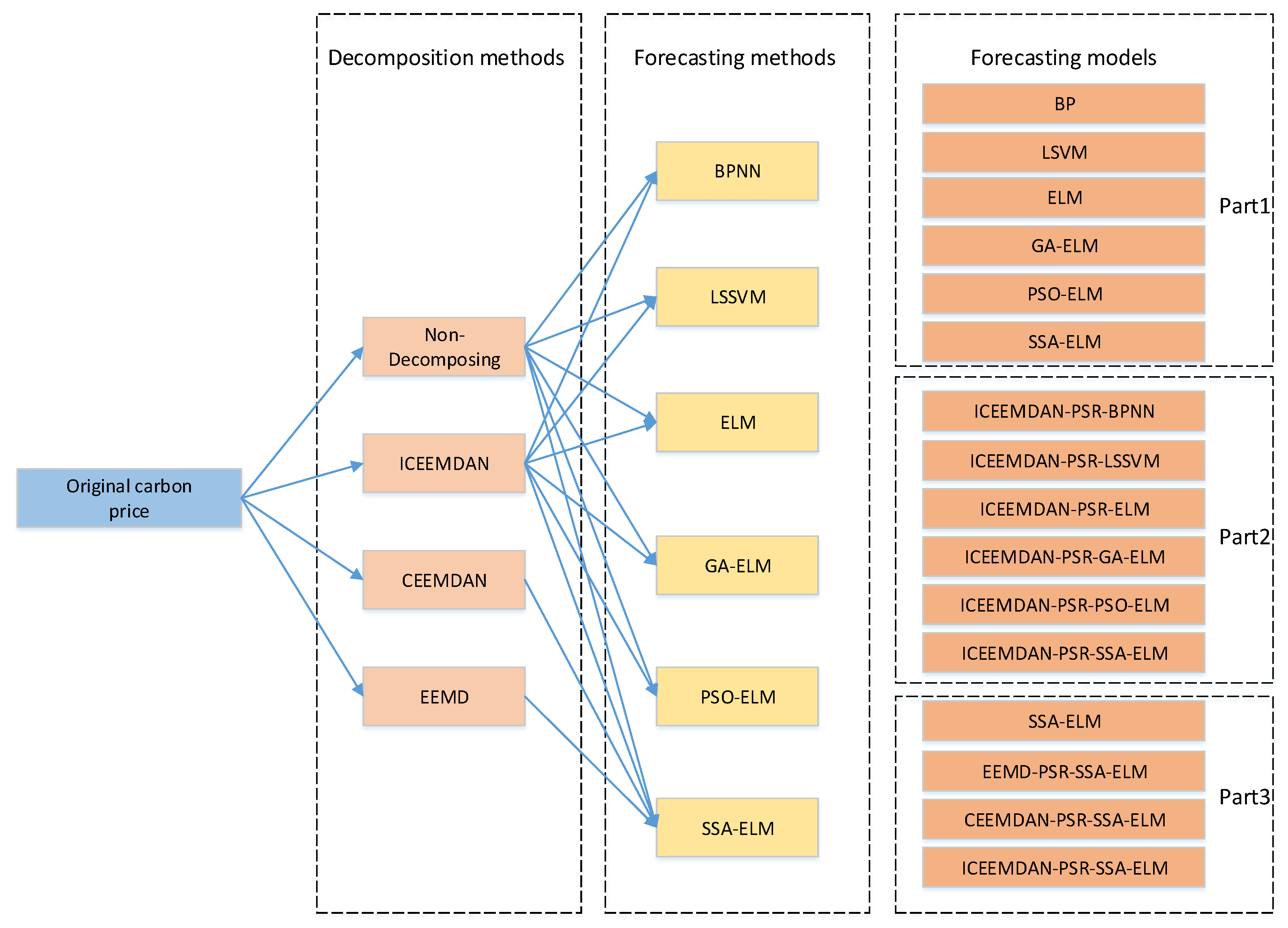
For the purpose of illustrating the necessity and superiority of the proposed hybrid model in this study, the contrasting framework is given in Figure 2. In part 1, the BP, LSSVM, ELM, GA-ELM, PSO-ELM, and SSA-ELM models were contrasted to verify the necessity of the optimization method and the superiority of optimizing ELM by SSA. In part 2, the ICEEMDAN-PSR-BP, ICEEMDAN-PSR-LSSVM, ICEEMDAN-PSR-GA-ELM, ICEEMDAN-PSR-PSO-ELM, and ICEEMDAN-PSR-SSA-ELM models were compared to verify the availability of the ICEEMDAN algorithm; meanwhile, the advantage of using the SSA-ELM model is further verified. In part 3, the SSA-ELM, EEMD-PSR-SSA-ELM, CEEMDAN-PSR-SSA-ELM, and ICEEMDAN-PSR-SSA-ELM models were contrasted to verify the advancement of ICEEMDAN and the essential importance of decomposing the carbon price.

4. Empirical Analysis

4.1. Data Analysis

The daily transaction prices of the Hubei, Beijing, and Guangdong carbon markets were selected in this paper for analysis. Data are from China carbon trading website (http://www.tanjiaoyi.com/). The carbon price sequence and descriptive statistics are shown in

Table 1. Carbon price sequence and descriptive statistics.

Carbon Market	Data Period of Carbon Price (Month/Day/Year)	Data Period of Test Data (Month/Day/Year)	Number of Test Data (Data Type)	Statistical Descriptions
				Mean	Maximum	Minimum	Std. Dev.	Jarque-Bera	Prob.
Hubei	06/30/2016–04/30/2020	06/17/2019–04/30/2020	180 (daily)	22.23	53.85	10.07	8.19	76.99	0.00
Beijing	08/10/2016–04/30/2020	07/29/2019–04/30/2020	180 (daily)	62.83	87.50	30.32	14.33	75.98	0.00
Guangdong	05/27/2016–04/30/2020	07/29/2019–04/30/2020	180 (daily)	17.66	30.84	8.10	5.74	99.02	0.00

. Taking Hubei as an example, the Hubei carbon price sample covers the period from 30 June 2016 to 30 April 2020, with 900 total data points, excluding public holidays. This paper uses an 8:2 ratio to select the training set and the test set. The fluctuation diagram of daily carbon prices about the Hubei, Beijing, and Guangdong carbon markets of China is shown in Figure 3.

Table 2. ADF test results.

Carbon Price	Stat	Prob.	1% Level	5% Level	10% Level
Hubei	−1.40948	0.5788	−3.43745	−2.86456	−2.56843
Beijing	−0.40777	0.5367	−2.56754	−1.94118	−1.61646
Guangdong	−0.76168	0.8287	−3.43742	−2.86455	−2.56843

and

Table 3. BDS test results.

Carbon Price	M-Dimensional Space
	2		3		4		5
	Stat	Prob.	Stat	Prob.	Stat	Prob.	Stat	Prob.
Hubei	0.1866	0.000	0.3187	0.000	0.4092	0.000	0.4707	0.000
Beijing	0.1839	0.000	0.3099	0.000	0.3953	0.000	0.4519	0.000
Guangdong	0.1931	0.000	0.3298	0.000	0.4253	0.000	0.4916	0.000

respectively show the Augmented Dickey-Fuller (ADF) test and Brock-Dechert-Scheinkman (BDS) test results. From the ADF test result, we can see that the critical values of the three levels are all below the test value, and the p-value, 0.5788, is greater than 10%, indicating that the Hubei carbon prices series is non-stationary. When the embedding dimension is 2–5, the BDS test result shows that the p-value are all 0, indicating that the carbon prices series of Hubei is nonlinear.

4.2. Data Processing

It is very necessary to decompose the Hubei carbon price series in view of the nonlinear and non-stationary properties verified by the ADF and BDS tests. The original series was decomposed into eight IMFs and one residual (R) by ICEEMDAN, and the result are indicated by Figure 4. For the sake of further demonstration, the performance of ICEEMDAN, CEEMDAN, and EEMD were introduced concomitantly to process carbon price. The decomposition results are given in Figure 5 and Figure 6.

The frequency of IMFs was ranked from high to low, and the high frequency sequence fluctuates relatively randomly, mainly affected by market supply and demand factors. The low frequency series have certain periodic fluctuation characteristics, mainly affected by market policies and macroeconomics. The residuals show the overall upward trend of the carbon price series. The IMFs show a simpler structure, greater volatility, and stronger regularity over the original carbon price series, which is more conducive to the further completion of carbon price forecasts.

4.3. Lempel–Ziv Complexity Algorithm

The result that was obtained by the Lempel–Ziv complexity algorithm can indicate the complexity of the time sequence [48].

The Lempel–Ziv algorithm was employed to calculate the complexity of each carbon price subsequence. We can clearly see that as the frequency of the decomposed subsequence changes from high to low, the complexity of each subsequence decreases in turn from Figure 7, which proves the effectiveness of the Lempel–Ziv algorithm. The similarity between the components is judged according to the result of the complexity calculation, and the sequences with analogical complexity will be recombined into a new subsequence (Subs).

The specific method is to refer to the identification model mentioned in the article [19] and make corresponding changes in combination with the research of this article. That is, the critical value is set to 0.6. From the results in

Table 4. Reconstruction results of Hubei carbon price subsequence.

Methods	Sub1	Sub2	Sub3	Sub4	Sub5
ICEEMDAN	IMF1	IMF2	IMF3	IMF4, IMF5, IMF6	IMF7, IMF8, IMF9
CEEMDAN	IMF1	IMF2	IMF3	IMF4, IMF5, IMF6, IMF7	IMF8, IMF9, IMF10
EEMD	IMF1	IMF2	IMF3	IMF4, IMF5	IMF6, IMF7, IMF8, IMF9

, through calculations, the IMF1, IMF2, and IMF3 components obtained by the ICEEMDAN decomposition method are divided into the high-frequency part of the carbon valence sequence. Because the high-frequency part has complex characteristics, it is independent as a new subsequence; the subsequences are Sub1, Sub2, and Sub3. The complexity values of IMF7, IMF8, and IMF9 are less than 0.1, indicating that their complexity is relatively low, representing the trend of the carbon price series and grouping them into a new subsequence Sub5. The remaining subsequences, IMF4, IMF5, and IMF6, represent the low-frequency part of the carbon valence sequence and form a new subsequence (Sub4). The results after reconstruction are shown in Table 4. Figure 8 shows the reconstructed subsequence trend graph.

4.4. Input Variable Selection

The method of phase space reconstruction when predicting chaotic time series has been adopted by many scholars [49,50]. This paper applies chaos prediction theory to carbon price prediction. The premise of the phase space reconstruction of the carbon price subsequence is to calculate the two main parameters, delay time $\tau$ and embedding dimension $m$, by calculating the Maximum Lyapunov index (MLYE) for determining whether the subsequence is chaotic; the results are shown in

Table 5. Parameters $\tau ,m$ and the results of MLYE.

Methods	Index	Sub1	Sub2	Sub3	Sub4	Sub5
ICEEMDAN	$\tau$	2	2	3	13	5
	$m$	12	8	8	5	3
	MLYE	0.0463	0.0729	0.0523	0.0288	−328.7958
CEEMDAN	$\tau$	3	1	2	8	11
	$m$	7	7	8	6	3
	MLYE	0.1377	0.1398	0.0697	0.035	−328.784
EEMD	$\tau$	5	2	3	16	6
	$m$	5	10	6	4	5
	MLYE	0.5136	0.0546	0.0811	0.0715	−327.9718

.

From Table 5, it is clear that the MLYE of Sub1, Sub2, Sub3, and Sub4 are all greater than 0, indicating that Sub1, Sub2, Sub3, and Sub4 are chaotic time sequences. In contrast, the MLYE of Sub5 are all below 0, indicating that Sub5 is a non-chaotic time series and that other methods are needed to confirm the input samples of the prediction model. The application of PACF is used to gain the input variables of the prediction model in this study. Figure 9 shows the PACF values within the 95% confidence interval. According to the PACF results of subsequences, the input combination variables for each subsequence were obtained as shown in

Table 6. PACF results of the Hubei carbon price.

Subseries	Input Combination
	ICEEMDAN	CEEMDAN	EEMD
Sub5	$x_{t-1}$	$x_{t-1}$	$\begin{array}{l}{x}_{t-1},x_{t-2},x_{t-3},x_{t-4},x_{t-5}\\ x_{t-6},x_{t-7},x_{t-8},x_{t-9},x_{t-10}\end{array}$

.

4.5. Evaluation Indicators

In order to evaluate the accuracy of the prediction model, this article selects four common error judgment indicators, namely, the average absolute error (MAE), the mean absolute percentage error (MAPE), the root mean square error (RMSE), and the coefficient of determination ($R^2$). Among them, the smaller the MAE, MAPE, and RMSE, the better the model prediction accuracy, and the closer $R^2$ is to 1, the better the model fitting effect will be [51]. The calculating equation of these indicators are as follows:

$$MAE=\frac{1}{n}{\displaystyle \sum _{i=1}^n\left|y_i-\widehat{y_i}\right|}$$

(10)

$$MAPE=\frac{1}{n}{\displaystyle \sum _{i=1}^n\left|\frac{y_i-\widehat{y_i}}{y_i}\right|}\times 100\%$$

(11)

$$RMSE=\sqrt{\frac{1}{n}{{\displaystyle \sum _{i=1}^n\left(y_i-\widehat{y_i}\right)}}^2}$$

(12)

$$R^2=1-\frac{{\displaystyle {\sum }_{i=1}^n{\left(y_i-\widehat{y_i}\right)}^2}}{{\displaystyle {\sum }_{i=1}^n{\left(y_i-\overline{y_i}\right)}^2}}$$

(13)

In addition, the Diebold–Mariano (DM) test was introduced for evaluating the prediction performance between the two models. The DM test null hypothesis $H_0:E\left[L(e_t^1)\right]=E\left[L(e_t^2)\right]$ indicates that there is no significant difference between the two prediction methods, and the alternative hypothesis $H_1:E\left[L(e_t^1)\right]\ne E\left[L(e_t^2)\right]$ indicates that there is a significant difference between the two prediction methods. The test statistics are defined as:

$$DM=\frac{{\displaystyle \sum _{t=1}^T\left[L(e_t^1)-L(e_t^2)\right]/T}}{\sqrt{{\lambda }^2/T}}{\lambda }^2$$

(14)

where ${\lambda }^2$ represents the estimated variance of $\left[L(e_t^1)-L(e_t^2)\right]$.

5. Forecast Results and Discussion

5.1. Forecast Results of Hubei Carbon Price

It is worth emphasizing that several other predictive models were selected for comparative analysis and for verifying the superior predictive performance of the proposed model, including three decomposition methods (ICEEMDAN, CEEMDAN, EEMD) and six prediction models (BP, LSSVM, ELM, GA-ELM, PSO-ELM, SSA-ELM).

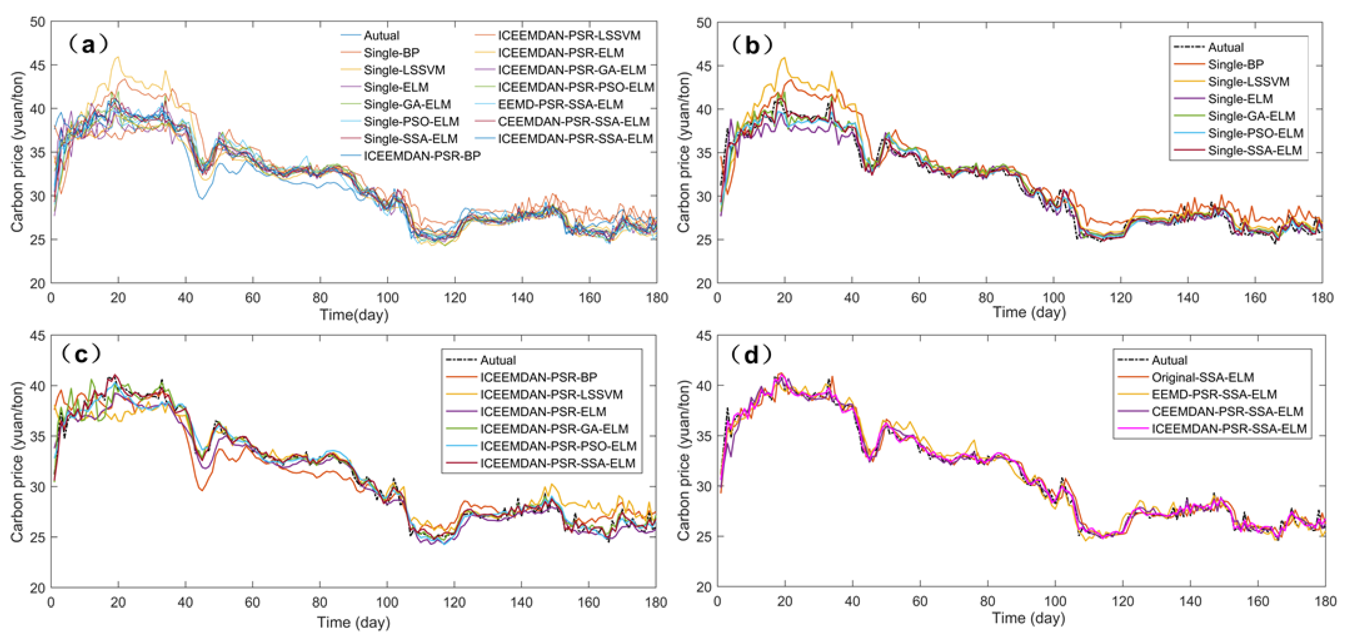
The prediction results of 14 prediction models were given in Figure 10a. For analyzing the results more concisely, (b), (c), and (d) show the prediction results of single forecast models, the same decomposition method with different prediction models, and the different decomposition methods with the same forecast model, respectively.

Table 7. Prediction evaluation indicators for 14 models (Hubei).

Models	${\mathit{R}}^2$	RMSE	MAPE	MAE	DM Test
BP	0.91	1.98	5.19%	1.61	8.3203 **
LSSVM	0.93	1.89	3.98%	1.32	6.7239 **
ELM	0.95	1.13	2.59%	0.83	6.1968 **
GA-ELM	0.95	1.11	2.55%	0.80	4.8548 **
PSO-ELM	0.96	1.01	2.23%	0.70	4.5098 **
SSA-ELM	0.97	0.87	2.08%	0.64	7.0560 **
ICEEMDAN-PSR-BP	0.91	1.46	3.61%	1.13	6.3786 **
ICEEMDAN-PSR-LSSVM	0.94	1.38	3.17%	0.97	5.2995 **
ICEEMDAN-PSR-ELM	0.97	0.97	2.26%	0.73	6.3490 **
ICEEMDAN-PSR-GA-ELM	0.98	0.66	1.36%	0.44	3.0308 **
ICEEMDAN-PSR-PSO-ELM	0.98	0.64	1.61%	0.51	4.9907 **
EEMD-PSR-SSA-ELM	0.98	0.65	1.64%	0.51	4.9285 **
CEEMDAN-PSR-SSA-ELM	0.99	0.58	1.26%	0.40	2.2830 *
ICEEMDAN-PSR-SSA-ELM	0.99	0.42	1.06%	0.32	——

** and * Indicates the 1% and 5% significance level respectively.

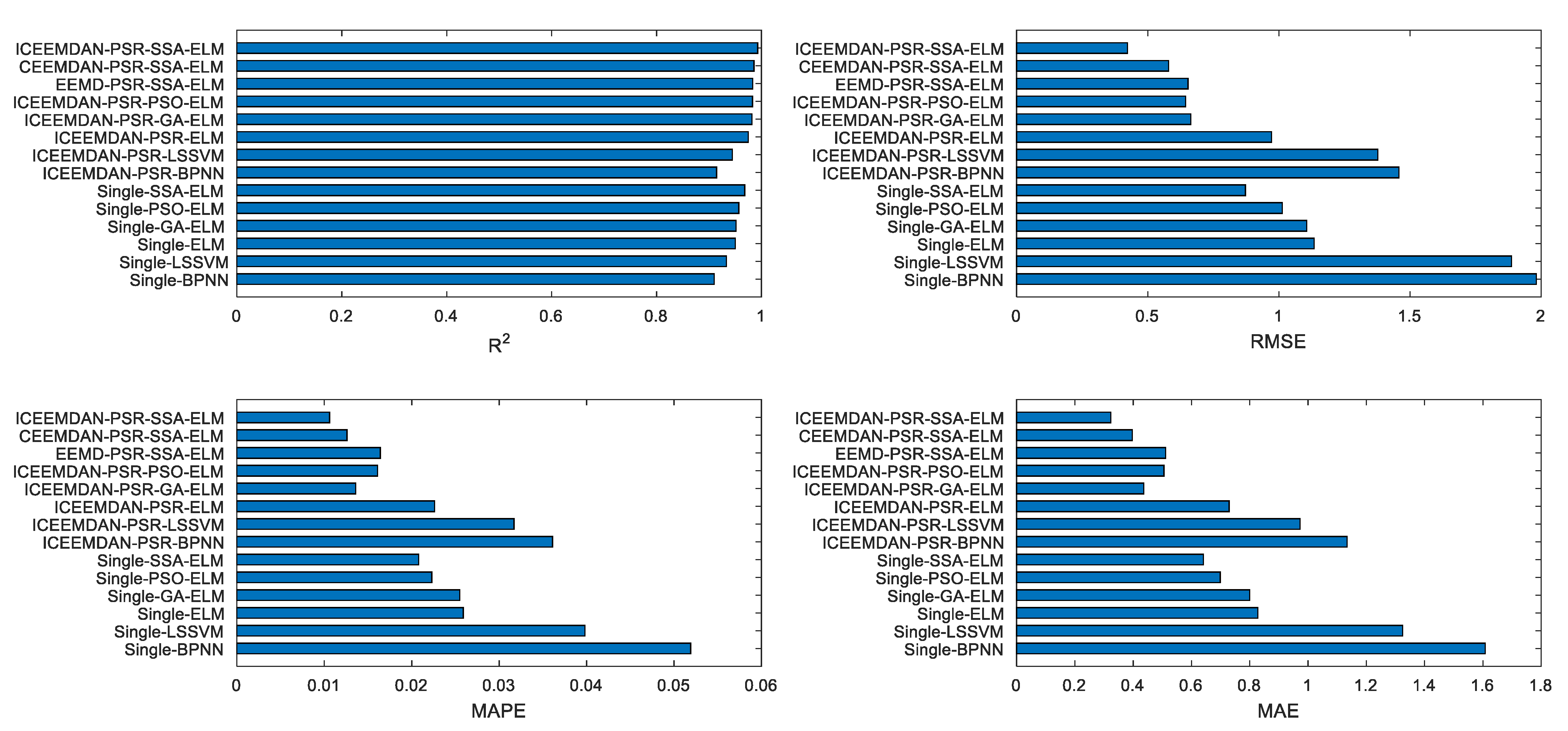
shows the error values and DM test results of the 14 prediction models. Figure 11 shows the $R^2$ RMSE MAPE MAE parallel model values. Combining Figure 10 and Figure 11 and Table 7, the following conclusions can be drawn:

Among the 14 prediction models, the results obtained by using ICEEMDAN-PSR-SSA-ELM are more fitted to the original data. The RMSE, MAPE, and MAE values are 0.42, 0.01, and 0.32, separately, which are smaller than other prediction models. $R^2$ is 0.99, which is greater than other forecasting models. These data indicate that the ICEEMDAN-PSR-SSA-ELM model has better stability and accuracy and can be well applied to carbon price prediction.

The prediction results of SSA-ELM were more fitting for the original carbon price series compared with BP, LSSVM, ELM, GA-ELM, and PSO-ELM. The MAE, MAPE, and RMSE values are 0.64, 0.02, and 0.87 separately, which are small compared to other single models, and $R^2$ is 0.97, which is greater than other single forecasting models. These data indicate the superior prediction performance of SSA-ELM. In addition, we find that the prediction performance of ELM is superior to the BP, LSSVM; the optimized ELM, GA-ELM, PSO-ELM, and SSA-ELM are superior to the Single-ELM; and the SSA-ELM has the best prediction performance, which indicates that it is necessary to optimize the parameters of ELM by SSA.

The carbon price series processed by ICEEMDAN and PSR were predicted with six prediction models. The results indicate that the decomposed carbon price prediction results are superior to the results of the single model without decomposition. The reason is that the carbon price is non-stationary and nonlinear; when the single model is directly used for prediction, there will be large errors, which indicates the necessity of using carbon price decomposition.

We compared ICEEMDAN-PSR-SSA-ELM with CEEMDAN-PSR-SSA-ELM, EEMD-PSR-SSA-ELM, and Single-SSA-ELM models. The error values of ICEEMDAN-PSR-SSA-ELM are all below other predictions, and $R^2$ is 0.99, which is greater than other prediction models, indicating that the data processing performances of ICEEMDAN is superior to the CEEMDAN and EEMD algorithms and that the predicted performance is better than that of the others under the same prediction method.

The results of the DM test can compare the prediction performance of two prediction models. The statistical results of the DM test based on the squared error loss function are shown in Table 7. The results show that the ICEEMDAN-PSR-SSA-ELM outperforms the 13 other prediction models at a 5% significance level. This shows that the predictive performance of the proposed model outperforms other benchmark models.

5.2. Additional Forecasting Cases

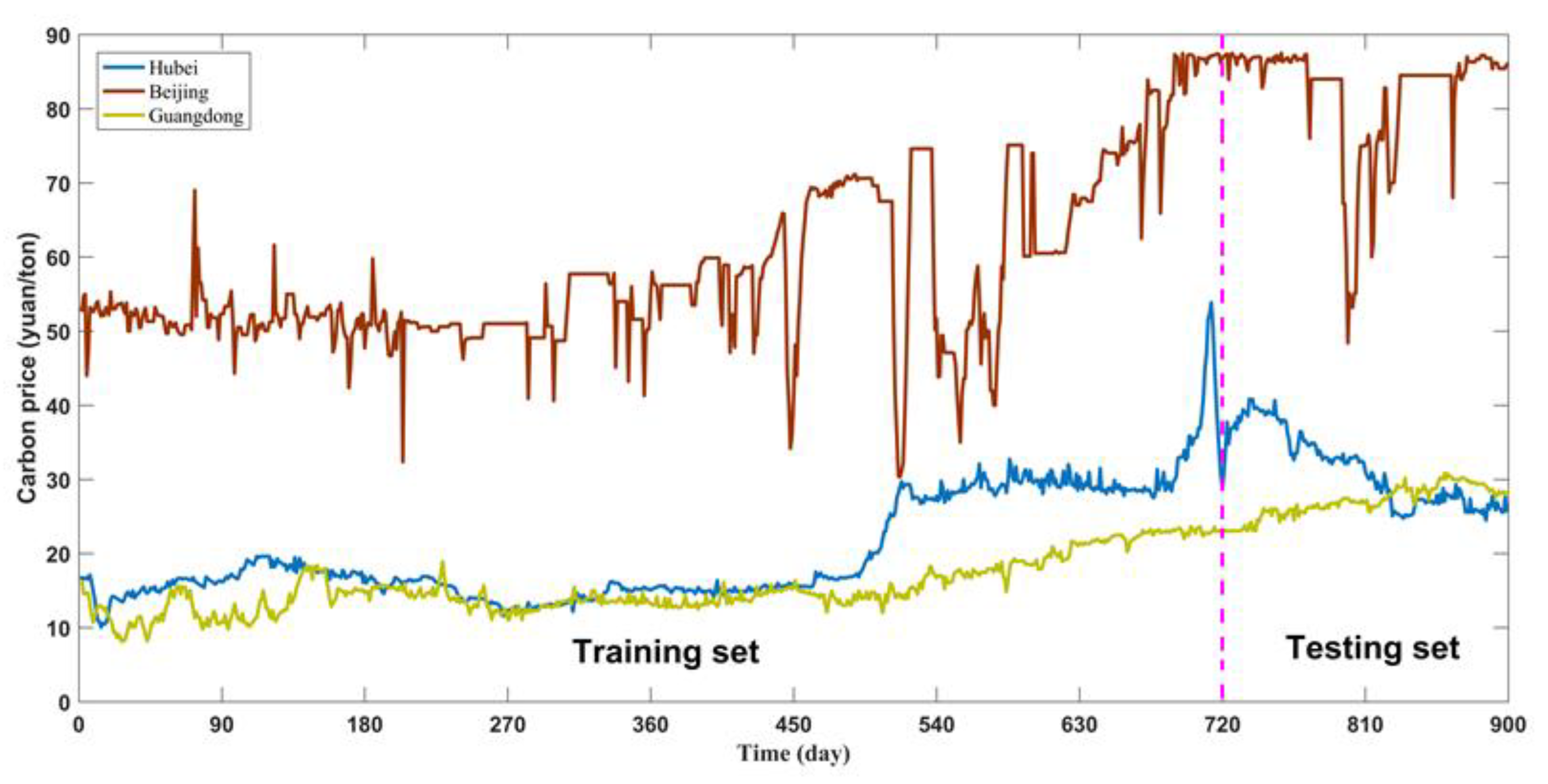
For the purpose of verifying the adaptability of the model, this paper selects representative Beijing and Guangdong carbon markets for carbon price prediction. The data information and description statistics are shown in Table 1, Table 2 and Table 3. The specific forecasting steps are similar to the Hubei carbon price forecast. The evaluation indicators of the 14 prediction models are shown in

Table 8. Prediction evaluation indicators for 14 models (Beijing and Guangdong).

Models	Beijing					Guangdong
	${\mathit{R}}^2$	RMSE	MAPE	MAE	DM Test	${\mathit{R}}^2$	RMSE	MAPE	MAE	DM Test
BP	0.81	3.63	3.22%	2.48	4.9894 **	0.91	1.97	5.93%	1.67	12.8389 **
LSSVM	0.83	3.26	2.36%	1.76	3.3515 **	0.93	1.21	3.62%	1.02	11.6401 **
ELM	0.84	3.18	2.23%	1.67	3.2984 **	0.93	0.95	3.04%	0.84	12.8216 **
GA-ELM	0.84	3.14	2.09%	1.53	3.1370 **	0.93	0.59	1.68%	0.45	7.9539 **
PSO-ELM	0.84	3.06	2.08%	1.49	3.0716 **	0.94	0.50	1.38%	0.37	6.2123 **
SSA-ELM	0.86	2.92	1.89%	1.39	2.8124 **	0.95	0.47	1.26%	0.34	5.9067 **
ICEEMDAN-PSR-BP	0.90	2.84	2.52%	1.99	3.5285 **	0.93	1.44	4.29%	1.21	13.4184 **
ICEEMDAN-PSR-LSSVM	0.93	2.29	1.81%	1.31	3.7918 **	0.94	1.18	3.45%	0.97	12.2076 **
ICEEMDAN-PSR-ELM	0.94	1.93	1.59%	1.18	3.3905 **	0.95	0.68	2.01%	0.55	8.7469 **
ICEEMDAN-PSR-GA-ELM	0.96	1.55	1.20%	0.90	1.9987 *	0.96	0.43	1.32%	0.36	8.1537 **
ICEEMDAN-PSR-PSO-ELM	0.96	1.47	1.16%	0.88	2.9141 **	0.98	0.27	0.73%	0.20	3.2533 **
EEMD-PSR-SSA-ELM	0.96	1.63	1.44%	1.10	2.8890 **	0.97	0.35	0.98%	0.26	5.9214 **
CEEMDAN-PSR-SSA-ELM	0.96	1.59	1.27%	0.95	2.0273 *	0.98	0.27	0.73%	0.20	2.8078 **
ICEEMDAN-PSR-SSA-ELM	0.97	1.33	1.08%	0.82	——	0.99	0.23	0.63%	0.17	——

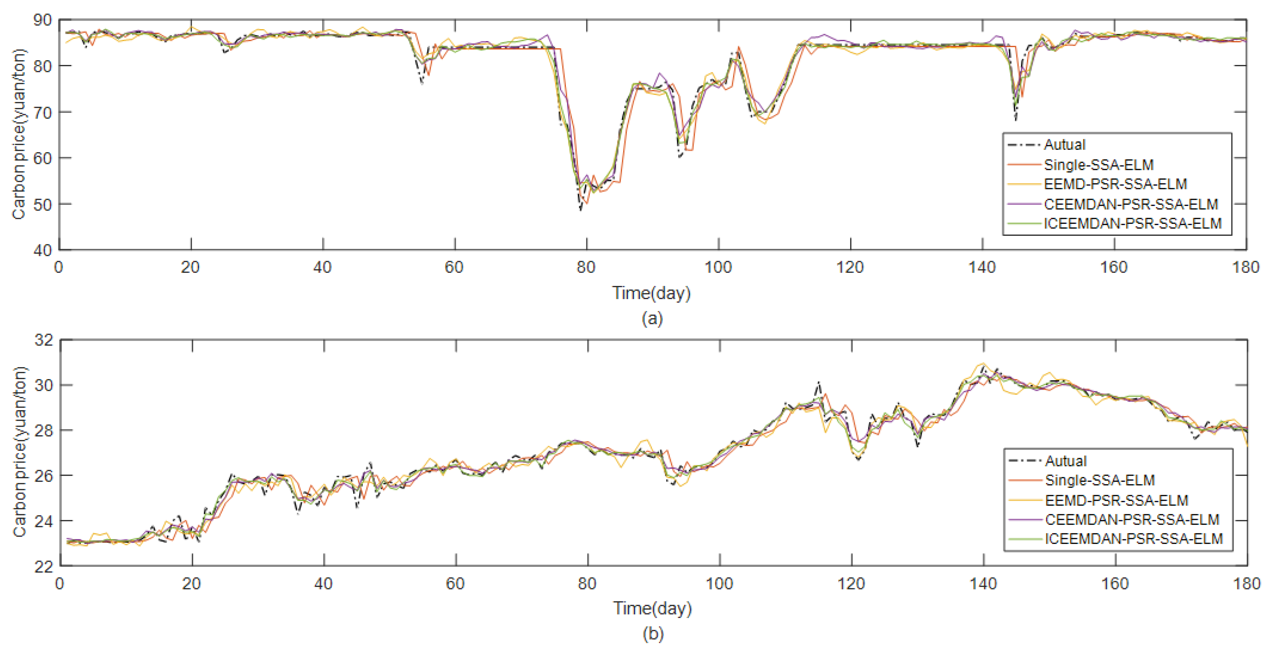
** and * Indicates the 1% and 5% significance level respectively.

. The results of the partial comparison model for Beijing and Guangdong are shown in Figure 12. According to the evaluation indicators results, and a conclusion similar to those in the previous section is obtained.

It is worth noting that the carbon price forecast of the Guangdong is more exact than those of Hubei and Beijing. The reason is that the volatility of the Guangdong carbon price series is relatively smaller. Similarly, the results of the Beijing carbon price forecasts have larger errors than those of Hubei and Guangdong, mainly due to the large fluctuations in the Beijing carbon price series. Additionally, we can conclude that the volatility of carbon prices will affect the accuracy of the prediction model.

Nonetheless, overall, the ICEEMDAN-PSR-SSA-ELM model studied in this paper is able to show superior forecasting performance for the carbon price forecasts of the Hubei, Beijing, and Guangdong exchanges. Combining the above research, this study can conclude that under the scenario where only historical carbon price data are considered, the accuracy of the proposed model reaches the best level, and the performance of the prediction model is more stable. This indicates that the mixed model is effective for carbon price prediction.

5.3. Discussion

The different decomposition methods (ICEEMDAN, CEEMDAN, and EEMD) were applied to test different prediction models (BP, LSSVM, ELM, GA-ELM, PSO-ELM, and SSA-ELM).

-

It can be found that the decomposition-integration strategy is more accurate than the carbon price prediction results obtained by a single prediction model.

-

In terms of the prediction model, the performance of the ELM model is better than BPNN and LSSVM model performances; the optimized ELM model is better than a single ELM mode. The performance of the ELM model optimized by the SSA algorithm is better than GA and PSO algorithms. This is because the SSA algorithm has strong competitiveness in search accuracy, convergence speed, and stability.

-

Compared with the CEEMDAN and EEMD models, ICEEMDAN can further eliminate noise and possible pseudo-modal problems. The Lempel–Ziv algorithm is adopted to reconstruct the subsequences. It can more effectively study the intrinsic characteristics of carbon price sequences, reducing, furthermore, the amount of calculation greatly. The input samples of the prediction model are selected by judging whether the subsequence is chaotic.

The experiment shows that this choice is more reasonable. The carbon price prediction results in Hubei, Beijing, and Guangdong indicates that the combined model has higher stability and precision, which is suitable for predicting carbon price. The contribution of this article is to innovatively apply the ICEEMDAN method to carbon price decomposition, and the experimental results verify its superior performance. Considering the chaotic nature of carbon prices, the internal characteristics of carbon prices can be better analyzed and the prediction accuracy improved. The ELM optimized by the SSA algorithm has a higher prediction accuracy.

The research results of this article will provide policy guidance for the implementation of a low-carbon economy, provide a basis for the establishment of a national integrated carbon market [52], provide a reference for the establishment of a personal carbon trading market [53,54,55], and provide a basis for the allocation of carbon allowances and changes in energy prices, thus providing a basis for future development plans of different industries such as energy and transportation.

6. Conclusions

This paper proposes a novel combination model to predict carbon prices. The model is first processed by the ICEEMDAN algorithm for data decomposition. Secondly, in order to better analyze the sequence regularity and reduce the workload, the Lempel–Ziv complex algorithm is introduced. Considering the chaotic characteristics of the carbon price time series, PSR and PACF are combined to determine the input variables of the forecasting model, and the SSA-ELM model is used for carbon price forecasting. It is proposed to apply this model to carbon price forecasts in Hubei, Beijing, and Guangdong and to compare the ICEEMDAN-PSR-SSA-ELM combined model with 13 other benchmark models. Research shows that the model has higher accuracy and efficiency. Based on the empirical results, the following conclusions can be drawn:

-

This paper conducts empirical research on three carbon markets and proposes 13 benchmark models for comparison. The result proves that the prediction effect of the ICCEMDAN-PSR-SSA-ELM model proposed in this paper is the best, which indicating that the proposed hybrid model can effectively improve the performance of carbon price prediction.

-

Because of the complex nature of the carbon price time series itself, data preprocessing in the early stage of forecasting is very necessary. The experimental results prove that ICEEMDAN is more effective than CEEMDAN and EEMD in dealing with carbon price series, and the decomposed IMF and residuals are more regular. At the same time, it is also very valuable to consider the chaotic characteristics of subsequences. The input feature selection of the prediction model is realized by combining PSR and PACF, which can significantly improve the prediction effect of the prediction model.

-

Compared with many carbon price prediction models, the performance of ELM is better than that of BP and LSSVM, which shows that the ELM model used in this paper is meaningful and more suitable as a carbon price prediction model.

-

Considering that the weights and thresholds of the ELM model may not be optimal, among the introduced optimization algorithms, the sparrow search algorithm proposed in this paper shows higher global search capabilities. The use of SSA to optimize the ELM model significantly improves the prediction effect of the predictive model and illustrates the importance of the optimization algorithm and the superiority of the sparrow search algorithm.

-

The decomposition-reconstruction-prediction-integration strategy can significantly improve the accuracy of carbon prices prediction. All combined forecasting models are better than a single forecasting model, which verifies the effectiveness of the proposed strategy.

Therefore, the experimental results show that the proposed prediction model is more suitable for carbon price prediction with nonlinear, non-stationary, and irregular characteristics. Accurate carbon price forecasts can help the government provide a basis for establishing a unified carbon market and strengthen market control when formulating low-carbon economic policies. In addition, it is a basis for enterprises to reduce investment risks and control market changes. In addition, the model can also be extended to other fields, such as wind speed forecasting, load forecasting, stock price forecasting, and so on.

However, this article still has certain limitations. First of all, this study only uses time series for research. Although the nonlinear, non-stationary, and chaotic characteristics of carbon price series are fully considered, the influence of the main factors affecting the change of carbon price on the prediction of the carbon price is not studied in depth. Secondly, this article only considers the empirical research of China’s carbon market.

Research can be carried out from the following aspects in the future. Firstly, the introduction of carbon price influence factors can be considered to further analyze the impact on the carbon price prediction. Secondly, research on the carbon market can be expanded and applied to the EU carbon market to verify the wide applicability of the model. Finally, based on the prediction model, an intelligent carbon price prediction system could be developed to provide a reference for policy-making and investment trading.