Abstract
To reduce frequent heavy air pollution, the Chinese government suspends clinker production during the heating season in most areas of the North, which is known as the Clinker Off-peak Production Policy. The questions regarding such a repressive production policy for environmental purposes are whether this policy is effective in reducing pollutants and whether the marginal cost is high. To explore these policy effects, a quasi-experiment is designed, taking advantage of spatial-temporal variations in policy implementation. With the triple-difference method and environmental satellite data, the effect on air pollution is estimated to be −1900 μg/m2 (~2%) of SO2 and −3200 μg/m2 (~10%) of NO2. With daily price information and the difference-in-differences method, the market effect is estimated to be an approximately 10% increase in annual sale prices. The marginal cost estimated through a back-of-the-envelope analysis is 32 k RMB yuan/ton SO2 or NO2, which is 24.88 times the pollutant discharge fee but which better reflects the pollutant shadow price.
1. Introduction
Seasonal heavy air pollution due to heating demand and comparatively low atmospheric capability in the autumn and winter [1,2] causes severe health damage and economic loss and has become China’s most significant environmental challenge [2,3]. Seeking sustainable development, China has put much effort into air pollution control, such as enacting several new air pollution policies that are included in the Air Pollution Prevention and Control Act (APPCA, 2013–2017) and the Three-year Plan to Fight Air Pollution (2017–2020) [4]. The Clinker Off-peak Production Policy (COPP) is a core policy among these measures in terms of industrial structure adjustment. The basic content is that the COPP suspends cement calcination during seasons in which centralized heating is supplied. The COPP is not only an air pollution control policy but may also affect the market supply-demand relationship, which has caused controversy over the policy’s effectiveness. An evaluation of the net effect on air pollution control and the market impacts can help further clarify the policy’s purpose and illustrate its actual effectiveness.
As an emergency pollution control measure, the suspension of heavy industrial production has a long history in practice. The previous studies on similar air pollution control measures can provide anticipation on the effectiveness of the enforcement of COPP. The Chinese government suspended and reallocated steeling/coking factories in Beijing in preparation for the 2008 Beijing Olympic Games. Chen et al. (2013) explore the effectiveness of the air pollution control measures in Beijing in the periods of preparation, during the Games, and 13 months after the Games, and find that the control measures significantly (p < 0.01) reduced the Air Pollution Index (API) of Beijing by around 35 during the Games and by around 20 after the Games. Further, they divide the whole area into 2.5 km cells and find the effect of closing one plant permanently to at best improve the Aerosol Optical Depth (AOD) within a 5 km radius by 0.091 units, which is much more effective than traffic control for a specific AOD area if considering the average road length within the cell [5]. Additionally, during the 2014 APEC summits (5–11 November) and 2015 Victory-day Parade (3 September), the Ministry of Environmental Protection published the Principles for Formulating the Air Quality Regulatory Program for Beijing and several provinces around Beijing which requires factories that fail to meet discharge standards to shut down. Li et al. (2017) find that both the Victory-day Parade regulation and APEC regulation are effective in air quality improvement. For example, the APEC regulation brought down the AQI by 35.9%, and the concentrations of PM2.5, PM10, SO2, NO2, and CO by 41.3%, 48.2%, 56.5%, 38.9%, and 35.5%, respectively [6]. Based on the effective enforcement of similar air pollution control measures in China, COPP is expected to have an effective and immediate air quality improvement effect.
Besides the effectiveness of COPP in air quality improvement, the second part of this paper intends to estimate the market effect. Existing literature has controversies over the market effect of environmental regulations, especially on energy-intensive industries. On the one hand, following the theory that environmental regulations internalize the environmental externalities into enterprises’ production, multiple empirical studies have found negative economic effects of environmental policies. For example, Becker and Henderson (2000) explore the unintended effects of the 1978 annual designation of county air quality attainment status and find that this reduced 26–45% births of polluting industries in nonattainment areas [7]. Greenstone (2002) studies the same environmental regulation and finds that there were approximately 590,000 jobs, $37 billion in capital stock, and $75 billion (1987 dollars) of output lost in pollution-intensive industries in nonattainment counties compared with attainment ones in the first 15 years of enforcement of Clean Air Act [8]. Linn (2010) conducts an event analysis with stock prices of the regulated firms and finds that the cap-and-trade program on NOx in the US caused a $25 billion reduction of the expected profit, which is mainly from the anticipation of the cost increase of coal generators in the regulated areas [9]. The negative effects of environmental regulations also include total factor productivity reduction and the threat to enterprises’ survival in energy-intensive industries [10,11]. On the other hand, Porter and his supporters argue that environmental regulations can improve productivity by promoting technology innovation [12,13].
However, the innovation effect of an environmental policy can take years to appear. Since COPP started in 2014, we focus only on the short-term effects. Following Testuji et al. (2018), this paper uses market price to explore the market effect. As COPP targets at cement industry, the market effect not only depends on policy design but also involves the market structure. Several studies discuss the effect of government interference on cement markets and the conclusions vary among different cement market structures. In highly concentrated industries, the output is far less than the optimal amount, and therefore the government’s repressive interference in production causes further welfare losses [14]. For example, Ryan (2012) exploits the structure model and estimates that the Clean Air Act has caused approximately 0.81 billion dollars in social welfare loss in the highly concentrated Portland cement industry in the US by increasing entry and exit costs [15]. However, in industries with excess production capacity, the government interference through removing excess production capacity may not cause a significant price effect or social welfare change if the remained capacity can still meet the market demand, such as the capacity reduction carried out in the Japanese Portland cement industry in the 1980s [16]. Industries with excess capacity are prone to attrition wars, which may result in a more serious waste of resources and social welfare loss, as in the case of the Norwegian Portland cement industry before 1968 [17]. This also shows the necessity and positive side of government intervention in the industry. The current Chinese Portland cement market exists excess production capacity, and the cement price experienced a valley in 2015. COPP reduces annual legal production days, which can increase the price through consumers’ anticipation of output reduction. Therefore, a significant price effect is expected of COPP.
Based on the literature review, we bring up two main hypotheses to be examined:
Hypothesis 1.
COPP can have an effective and immediate air pollution control effect.
Hypothesis 2.
As a government-determined production policy, COPP can cause a significant price increase in the clinker market.
To examine Hypotheses 1 and 2, the quasi-natural experiment method is employed and conducted with Triple Differences (DDD) and Difference-in-Differences (DD) estimators. Greenstone et al. (2009) argue that greater application of experimental and quasi-experimental techniques can identify efficient policies that increase social welfare [18]. Conducted through DDD and DD models, the quasi-natural experiment method can effectively eliminate estimation bias of policy effect from unobservable confounds. Main works that tend to isolate policy’s net effect include Auffhammer and Kellogg (2011) that comparatively analyze the effects on O3 reductions of three gasoline VOCs content policies in the US with DD and RD models [19]; Greenstone and Hanna (2014) that isolate the effectiveness of water protection policy and air pollution control policy in India with DD models [20], and so on. The spatial-temporal variations in the enforcement of the COPP creates an ideal quasi-natural experiment to study its net environmental effects. Different from the policies studied in the above literature, COPP has obvious seasonal variations. Therefore, besides two variations that come from the regulated cities and regulated years, the third difference, seasonal variation, is also compared in this paper. The application of DDD estimator follows Deschênes et al. (2017) that study NOx budget program (NBP). Since the cap-and-trade market operated only between May 1 and September 30, they use the DDD estimator to compare pollution, defensive expenditures, and health outcomes in the NBP participating and nonparticipating states, before versus after the first policy year, and summer versus winter [21]. Ignoring the seasonal variations will cause potential estimation bias in both cases.
To be noticed, a DD model is employed to estimate the price effect. The response of clinker/cement price to COPP is not as immediate as pollution discharge and the price effect can shift across seasons. Therefore, this paper compares clinker prices in COPP participating and nonparticipating cities, and before versus after the first policy year of each city with the DD model.
This paper is arranged as follows. Section 1 presents the introduction and a brief literature review. Section 2 introduces the policy background. Section 3 introduces the datasets and model specifications. Section 4 presents the regression results and further validation. Section 5 estimates the marginal cost of COPP through a back-of-the-envelope analysis. Section 6 concludes and provides policy implications.
2. Policy Background
Since the 1990s, China has experienced a huge expansion of its cement capacity along with its rapid economic growth and urbanization. According to the Ministry of Industry and Information (MII), there are 1240 clinker plants in mainland China with a total capacity of 5,922,513 tons/day, distributed across 304 prefecture-level cities as of December 2017. Appendix A, Figure A1 displays the total clinker capacity of each city, as well as the distribution and capacity of each clinker production line.
The calcination process in the cement industry accounts for the second-highest level of coal consumption in China, after only thermal power generation. According to The Cement Industry Total Coal Consumption Control Plan and Policy Research from the China Cement Association, in 2012, the total energy consumed in cement production equaled 207 million tons of standard coal, of which 96.6% was from coal-burning and electricity consumption. Excluding the air pollutants discharged from electricity generation, the clinker/cement industry emitted 1.09 million tons of SO2, 1.98 million tons of NOx, and 671,000 tons of dust, accounting for 5.7%, 11.9%, and 6.5% of total industrial emissions of those pollutants, respectively.
At the national China People’s Political Consultative Conference (CPPCC) held in March 2014, several CPPCC members from the publishing industry proposed implementing an off-peak production coordination mechanism for cement manufacture in Heilongjiang, Jilin, Liaoning, Hebei, and Inner Mongolia. They proposed suspending cement production during heating seasons when market demand is low and heavy smog frequently appears, to adjust cement supply-demand conflicts and improve air quality.
From June to July 2013, the Ministry of Industry and Information Technology (MIIT) conducted field investigations in the proposed regions and agreed on this proposal. Following its tradition of policy experimentation, China initiated four provincial COPP pilots in Xinjiang, Liaoning, Jilin, and Heilongjiang Provinces in 2014. In the following year, MIIT and the Ministry of Environmental Protection (MEP) jointly issued the “Notice on the Comprehensive Trial Implementation of Off-peak Clinker Production in the Northern Heating Region”. This was the first national document of the COPP, which imposed full COPP participation on all 13 provinces and 2 municipalities in the North. In October 2016, MIIT and MEP jointly issued the “2016–2020 Clinker Off-peak Production Announcement”, which formulates a preliminary plan for the COPP for 2016 to 2020. Beginning in the autumn of 2017, the regulatory targets expanded to include all building material, steel, and coking industries in “2 + 26” cities along the Tianjin-Beijing-Hebei air pollution transmission channel (This is detailed in a central official document, “2017–2018 Notice on the Industrial Sectors of “2 + 26” Cities to Carry Out Off-peak Production in Autumn and Winter”).
3. Data and Methods
3.1. Data
3.1.1. Explained Variables
Satellite air pollution data: For the explained variables, the SO2 and NO2 daily tropospheric column mass density (TCMD) were selected to represent air quality. SO2 TCMD is extracted from the time-averaged two-dimensional collections of MERRA2 which is a NASA atmospheric reanalysis for the satellite era (For the data download and Readme file, please search “M2T1NXAER_5.12.4” on the following website: https://disc.gsfc.nasa.gov/datasets) [22]. NO2 TCMD is from POMINO (For the data download and Readme file, please refer to https://ocean.pku.edu.cn/info/1038/3123.htm), an improved and validated NO2 data product based on OMI by Peking University [23]. The unit of each data is a density unit and converted to kg/m2. Data cleaning is conducted based on the data quality standards from the Readme files. The MERRA2 data does not need extra cleaning. The POMINO observations with a quality index below 0 and cloud rate bigger than 0.5 are dropped. The reading with a projected location nearest to the municipal center of a prefecture-level city (all less than 100 km (Considering the spatial resolution of satellite data, a 100 km radius is an operation-efficient range that can guarantee at least one observation is obtained for each city)) is used as the reading for that city.
Streets et al. (2013) review the capability of satellite data and present the summary of the major satellite instruments, their characteristics, and the chemical species they can detect. Among these satellite-based atmospheric component monitors, OMI is the most widely applied because of its long duty (2004–), high frequency (daily), and high resolution (13 km × 24 km) [24]. Several research organizations have modified OMI original data using local air mass factor and other parameters and developed level2 and level3 products. POMINO is one of these products.
The satellite-based air quality datasets are generally validated and applied in the atmospheric study but the introduction and application in the environmental economic study are not rich. However, Donaldson and Storeygard (2016) point out the main advantages of satellite data in economic study, which also can be cited to explain why using satellite data is better in this paper [25]: First, the access to obtain information by other means is difficult. There are no ground-monitored air quality data records that fully cover Chinese cities before May 2014, which has limited relative studies to a period after 2014. Since some cities began to implement COPP in 2014, using ground-monitored data will sacrifice the control observations before the policy year which is crucial for estimation accuracy. Second, satellite data has high spatial resolution and wide geographic coverage. Even if ground-monitored air quality data of most Chinese cities is available after 2014, the number of national ground monitoring stations is limited. The reads for some small cities come from the ground monitoring stations located in a nearby city. Also, many ground monitoring stations are far from the city center and therefore the reads are not within our interested area. Instead, the high spatial resolution of satellite-based data allows the choice of accurate observed locations and the wide geographic coverage allows reads for all cities. Other potential considerations include that the site choice of ground monitoring station is not independent of air pollution distribution [26], and the reads in some Chinese cities may be modified out of political pressure [27].
Clinker price data: Clinker prices are from the China Cement website, the largest website with information on the Chinese cement industry that regularly collects price and other information from the cooperative cement facilities, covering over 85% of all facilities. The data are of daily frequency and are available over the observation period 2010–2017, tagged with cement type, brand, manufacturer, and sales agent information. We match the price data with clinker line data via the manufacturer name to control for facility-level factors.
3.1.2. Explanatory Variable
The explanatory variable is a dummy variable indicating whether the observation is within a shutdown period. The specific shutdown dates for each city come from official documents and are verified by news from China Cement. When collecting COPP-relevant documents, we use a top-down approach; that is, we use central government documents first to find regulated regions and then provincial and municipal government documents to find more specific COPP plans, as all COPP-relevant documents are required to be publicly available by MIIT and MEP. The specific shutdown dates are based on the available plans from the lowest administrative level. The COPP proposal was initiated in March 2014, so “off-peak production” was used as a keyword, and 1340 pieces of news were found on the China Cement website. By going through all news items, extra cities that are not required to participate in the COPP by higher-level governments but actually joined independently were located, and the specific participation dates of all cities were verified.
After eliminating observations with either ambiguous shutdown dates or missing satellite data, 214 prefecture-level cities were kept in the treatment group. 27 cities first implemented the COPP in 2014. Then, 74, 33, and 80 new cities joined sequentially from 2015 to 2017. Appendix A, Figure A2 shows the policy year of cities on the map.
3.1.3. Control Variables
Socioeconomic variables: In the price effect estimates, the proportion of cement output to total output and fixed asset investments per capita are controlled for to account for market supply and demand impacts. The regressions also control for city-level characteristic variables, such as GDP per capita, the proportion of the secondary industry to total industry, and government expenditure per capita. The proportion of cement output is from the National Bureau of Statistics, and the other variables are from the Statistical Yearbook of Chinese Cities. Facility-specific variables, such as firm age, are from the China Cement website.
Weather variables: Weather information is used for control variables. The data are also from MERRA2, following the same data cleaning and averaging procedure as for the SO2 TCMD. Weather variables include temperature, precipitation, wind speed, and direction, all in daily averages.
The observation period for the above datasets is 1 January 2010, to 31 December 2017. The COPP is currently still in effect, but observations from after 2017 are eliminated because more industries have joined the program since then. Additionally, the COPP plans themselves have become more flexible, which means that actual implementation dates and capacities are hard to define. Table 1 lists the definition, units, and sources of all variables and Table 2 presents summary statistics of the variables.

Table 1.
Variable definition and data sources.
Table 2.
Summary statistics.
3.2. Methods
3.2.1. DDD Model Specifications
Since COPP is a seasonal policy, accurate estimation of its air quality effect requires isolating the air quality change during the corresponding dates rather than average air quality change throughout the year, which cannot be solved by DD estimator. Following Greenstone et al. (2012), this paper conducts a DDD model to identify the impact of COPP-regulated suspensions on air quality. The DDD estimator exploits three sources of variations: cities that implement the COPP and those that never implement the COPP, the years for each city before and after it implemented the COPP, and the months of facility shutdowns and those of production. In other words, the city-year-months of production suspensions are compared with those outside of the regulated suspension periods. The model is given as follows:
where icmy indicates the ith observation for each city-month-year. Y denotes the air pollution variable, including SO2 and NO2. Treat is the explanatory variable indicating the treatment status of each observation, and Treat = 1 when an observation is within the suspension dates defined by the city-year-month information; otherwise, Treat = 0. All three sets of two-way fixed effects should be included in the DDD operation. Due to the efficiency of our calculations, we control for three two-way fixed effects: the city-by-year fixed effects φcy, which account for all factors common to a city within a year; the month-by-year fixed effects ωmy for all factors common to a month and year; and the city-by-month fixed effects μcm for permanent differences in outcomes across city-months [21]. We also control for city fixed effects ρc, year fixed effects σy, and month fixed effects τm (The month fixed effects are not absorbed by the higher dimensional fixed effects, while the year fixed effects and the city fixed effects are absorbed by higher dimensional fixed effects [25]). In addition to the main fixed effects, we control for a set of variables to address annual, monthly, and weekly cycles in air quality, as well as their interactions with the weather variables. All regressions limit the sample to a balanced panel of city-month-years. The standard errors are clustered at the city-year level.
3.2.2. DD Model Specifications
The response of clinker price to COPP is not as immediate as the pollution discharge and the price effect can shift across seasons through consumers’ expectation of the output reduction. We estimate the annual average price effect of COPP rather than the effect that appears during certain months. We conduct the following DD model to compare the price difference in cities that implementing COPP versus those not implementing COPP, and years before the policy versus after:
where icy indicates the observation of ith facility in each city-year. Y denotes the annual clinker sale price. Treat indicates whether the observation is within the COPP treatment period, and Treat = 1 when the facility is within a suspension year; otherwise, Treat = 0. X’ is a vector of control variables, including city-level control variables such as GDP per capita, the ratio of the industry output value, fiscal expenditure per capita, foreign investment per capita, and the proportion of clinker output, as well as facility-level control variables such as facility age and facility age squared. We also control for city fixed effects ρc, and year fixed effects σy. The standard errors are clustered at the facility-year level.
To validate the DD model, the dynamic price effect is explored to observe yearly differences and examine the common trend assumptions between the two groups. The model specification is as follows:
where t gives the standard treatment year that ranges from −5 to 3, with 2014 as the base year. D indicates whether the observation in year t is in the treatment group (D = 1) or control group (D = 0). δt gives the dynamic effect coefficient of the COPP in year t. The other terms are the same as those in model (2).
The econometric process is conducted via STATA 16 software.
4. Results
4.1. Effect on Air Pollution
Figure 1 reflects air quality using SO2 (Panel A) and NO2 (Panel B) TCMDs within and outside of the shutdown period regulated by the COPP in Heilongjiang Province. For the years 2016–2017, Heilongjiang experienced clinker production suspension from 1 November to 31 March of the next year. In 2017 only, there were 3 suspensions conducted from May to September, and each was approximately 20 days. From Figure 1, both the SO2 and NO2 TCMDs during most of May–September 2017 were lower than those during the same period in 2016. The seasonal patterns support the feasibility of the DDD method for estimating the effect on air pollution control.
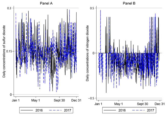
Figure 1.
A comparison of the within-year pattern of atmospheric pollutants between 2016 and 2017: Panel A daily SO2 and Panel B daily NO2 TCMDs, taking Heilongjiang Province as an example. The values were obtained from an OLS regression of SO2 and NO2 TCMD on six day-of-week indicators, weather variables, and a constant. The values in the graph are equal to the constant plus the regression residual. The graph depicts fitted values for the reference category (Monday). Daily TCMDs on the y-axis are measured in μg/m2.
Table 3 displays the regression results for the DDD regression and the robustness checks. Columns (1)–(4) use the SO2 TCMD as the explained variable and (5)–(8) use the NO2 TCMD. Columns (1) and (5), which include city fixed effects, year fixed effects, month fixed effects, and their two-way interaction, show that the COPP significantly reduced daily SO2 by 1762 μg/m2 and the daily NO2 TCMD by 2712 μg/m2, both at the 0.01 significance level. Columns (2) and (6), which additionally control for DOW, DOY, Season FE, Region FE, and their interactions, estimate the causal effect of the COPP on daily SO2 and NO2 TCMDs to be −1863 μg/m2 and −2807 μg/m2, respectively. Columns (3) and (7) add Weather and its interactions with DOW and DOY. Columns (4) and (8) add Trend as an extra control. There is an amplification of the coefficient of interest, γ, along with the introduction of additional control variables, which validates the choice of fixed effects used in this model. For the results of SO2, the robust standard errors are within the range of 230–250. The estimates are all significant at 1% level. R2 is around 0.6. For the results of NO2, the robust standard errors are within the range of 227–231. The estimates are all significant at 1% level and R2 reaches 0.14. The results are robust across models which indicates the credibility of the estimations. The COPP’s causal effects on the daily SO2 TCMD can be fairly accepted as −1900 μg/m2 and those on the daily NO2 TCMD as −3200 μg/m2.
Table 3.
The effects of the Clinker Off-peak Production Policy (COPP) on air pollution.
4.2. Effect on Clinker Price
The questions regarding government interference with clinker production are the extent to which such interference affects market power and whether it causes significant social welfare loss. The product sale price is a key index for measuring social welfare changes [16]. To explore the market effect, the plant-level daily clinker sale price and model (2) are employed. Table 4 shows the regression results. Column (1) controls for total investments in fixed assets averaged over the population and the proportion of cement output to total output for each city. Column (2) adds GDP per capita, government fiscal expenditure, and the ratio between the gross value of secondary industry production and GDP. Column (3) additionally controls for facility age and the square of facility age. The robust standard error is around 0.19 and R2 is around 82%. The estimates of the price effect are significant at the 1% confidence interval, and the effect of the COPP on annual clinker prices is approximately 10%. This result is robust across regressions. The above statistical parameters validate the reliability of the models.
Table 4.
The effects of the COPP on the annual average of clinker sale prices.
We also estimate the dynamic effect of the COPP on clinker prices using model (3). The regression results are plotted in Figure 2. We find that in the pretreatment period, these estimates are approximately 0 and insignificant. Immediately after the COPP was implemented, there was a clear increase in the estimated effect, and it remained significantly positive. This result demonstrates no differential time trend before the treatment and validates the DD results.
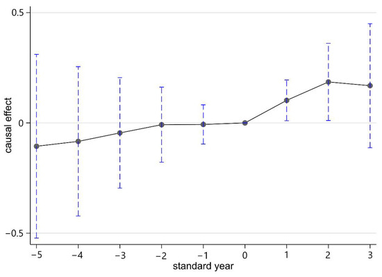
Figure 2.
Common trend analysis of the COPP’s effects on clinker prices.
4.3. Placebo Test
This subsection intends to further examine if the significant effects are caused by potential unobserved variables by employing a placebo test. The idea of a placebo test is that if the effects that the model estimates are due to unobservable variables, the distribution of the results from randomized trials must be very different from the standard normal distribution. In the spirit of Chetty et al. (2009) and Martin et al. (2017), we first keep only cities in the treatment group and then randomly assign them a year as they started to implement COPP. Then regressions are conducted to estimate the effect of the placebo policy [29,30]. Since the policy event is not real, the estimate is expected to be insignificant. This exercise is repeated 200 times. For each iteration, we run the following regressions for each outcome of interest:
The randomly assigned treatment is distinguished from true treatment by year to avoid confounding.
Table 5, Panel A shows the results from one of the 200 placebo runs, while Panel B summarizes the number of runs that were significantly above or below 0 at the 10% level for each outcome of interest. For most outcomes, 20 or fewer runs were significant at the 10% level. Overall, 7.5% of the NO2 results were significant, and 0 of the SO2 results were significant. The clinker price outcome did have 26 runs (13%) that were significantly different from 0, 24 of which were negative, which is the opposite direction from the true results. Panel C shows an empirical cumulative distribution function (CDF) from the 200 placebo results for NO2, SO2, and clinker price. As expected from a successful placebo test, the true coefficients for the effects on NO2 and SO2 are at the far left of the CDF, and the true coefficient for the effect on clinker price is at the far right of the CDF. Therefore, the placebo test validates that the pollutant reduction and price increase are caused by the COPP.
Table 5.
Placebo test.
5. Back-of-the-Envelope Analysis
5.1. Total Pollutant Mass
Satellite pollutant data in this paper gives the daily mass over the projected area of the tropospheric air column, which can theoretically be integrated across city areas and shutdown days to estimate the total mass reduction caused by the COPP. The integration of TCMD has been widely used to retrieve pollutant burden and emission rates via top-down methods, such as Beirle et al. (2011), and Laughner and Cohen (2019) [31,32]. The daily SO2 and NO2 TCMD reduction coefficients are equal to −1.9 kg/km2 and −3.2 kg/km2, respectively. The results show the impact of COPP on the air quality at city centers. However, considering that the clinker facilities in different cities are randomly distributed around city centers, it is reasonable to assume in this back-of-the-envelope analysis that COPP has an equal impact on air quality across the city. Integrations are conducted using the average effect coefficients, the municipal area (from China City Yearbook), and the number of shutdown days within the whole year for those cities that participated in the COPP from 2014 to 2017. For comparison with market costs, the total mass reduction is converted to province-year level, as shown in Table 6. The average annual tropospheric SO2 mass reduction was 8.7, 22.5, 32.8, and 45.9 kt per province-year for 2014–2017. The average annual tropospheric NO2 mass reduction was 14.6, 37.9, 55.2, 77.3 kt per province-year for 2014–2017.
Table 6.
Results of the back-of-the-envelope analysis.
5.2. Market Cost
The definition of market cost here is the part of social welfare change caused by the price effect, which is the extra money consumers paid to purchase the same amount of clinker that is caused purely by the COPP or could be regarded as the cost the consumers paid to reduce tropospheric pollutant mass through the COPP. The market cost for each province is the price increased multiplied by the clinker output each year. The average market costs are 535.97, 662.89, 731.25, and 1150.16 million RMB yuan per province-year for 2014–2017, which equals 82.46, 101.98, 112.5, and 176.95 million US dollars.
5.3. Marginal Cost
After balancing the province-year pollutant reduction and market cost data, 24 province-year observations are kept to further calculate the unit cost of SO2 and NO2 reductions through the COPP, as shown in Table 6. The average cost of reducing each ton of tropospheric SO2 or NO2 through the COPP was 32 k RMB yuan from 2014–2017 (Since the pollution discharge fee is the same for SO2 and NOX, the value of a reduction of one unit of SO2 and NOX is assumed to be identical here. The ratio of NOX to NO2 in the atmosphere is not addressed here because the uncertainty in the back-of-the-envelope analysis is larger than that). China has established 11 pilot provincial markets for trade in pollutant permits since 2007 and adjusted pollution discharge fees after 2007. The unit prices for pollutant discharge and pollutant permits can both provide a reference for the marginal price of pollutant reduction. Table 6 gives the provincial discharge fees, which range from 1.26–2.4 k RMB yuan/ton [33]. In other words, the marginal cost of pollutant reduction through the COPP is 24.88 times the pollutant discharge fee. The price of pollution permits ranged from 1–15 k RMB yuan/ton between 2001–2017 among pilot provinces. The SO2 shadow price between 2011 and 2014 is reported in the literature to be approximately 72.5 k RMB yuan/ton [34]. Additionally, for the province with the highest permit trade price, Hunan, the shadow prices reported in the literature are 3.02 k RMB yuan/ton for SO2 and 58.09 k RMB yuan/ton for NOX [35]. Therefore, the marginal cost of reducing pollutants through the COPP is higher than the marginal costs given by discharge fees and pollution permits but is within the range of rational shadow prices given in the literature.
6. Discussions and Policy Implications
The main findings of this article are concluded as follows: (1) the net of the COPP effect on pollution is −1900 μg/m2 of SO2 and −3200 μg/m2 of NO2; (2) the average tropospheric SO2 mass reduction is 8.7, 22.5, 32.8, and 45.9 kt per province-year from 2014–2017 and the average tropospheric NO2 mass reduction is 14.6, 37.9, 55.2, 77.3 kt per province-year from 2014–2017; (3) the effect of the COPP on annual sale prices is approximately 10%, which caused consumers to pay extra costs of 535.97, 662.89, 731.25, and 1150.16 million RMB yuan per province-year from 2014–2017, or 82.46, 101.98, 112.5, and 176.95 million US dollars; and (4) the marginal cost of pollutant reduction through the COPP is 32 k RMB yuan/ton, which is 24.88 times the pollution discharge fee and is higher than the discharge permit trade price, but is closer to pollutant shadow prices estimated in the literature.
First, the air pollution control effect implies that the enforcement of “Chinese style” air pollution control policy under the leadership of the Chinese government is effective and immediate. This conclusion is generally consistent with the findings of effectiveness analysis of air pollution control policies of China. For example, Wang et al. (2021) find that the central environmental inspection mechanism of China significantly improved air quality and argue that this system has had an immediate effect in general [36]. The literature has found that the effectiveness of air pollution policy enforcement relies largely on public concern under a weak environmental institution. However, for the case of China, the literature has argued that the focus of the Chinese government plays a significant role in the effectiveness of air quality improvement [5]. Therefore, it is of great significance to explore how the Chinese government design and implement air pollution control policies, especially those of the “Chinese style”, to promote effective environmental governance and sustainable development.
Second, the market effect implies that the administrative air pollution control measures in energy-intensive industries increase the market price and possibly bring a higher marginal cost of air pollutant reduction compared with market-based measures. Similar works that study air pollution policies of China mainly focus on the policy effectiveness and seldom estimate the policy cost. For example, Li et al. (2020) estimate the benefits of fuel standard upgrade but fails to estimate the cost. They point out that the economic realities are not transparent for oil refineries and the profit estimate is rough [37]. In this paper, we find that the marginal cost of COPP is much higher than the pollution discharge tax rate. Fowlie et al. (2016) calculate the social benefits of carbon abatement with emission tax rate and argue that reductions in product market surplus and allocative inefficiencies due to market power in the US cement market counteract the benefits [38]. From this view, we argue that COPP requires government and residents to assign a high marginal value to pollutant reduction to avoid the potential cost-and-benefit distortion. In other words, the sustainability of COPP as an air pollution control policy depends on the government’s and the resident’s willingness to pay.
Therefore, the performance of the COPP generates the following policy implications for the environmental governance in energy-intensive industries. (1) Repressive production policies are an effective and immediate measure for reducing tropospheric pollutant mass and are therefore of high practical value for emergency control of heavy pollution. (2) Although the literature argues that the government’s repressive production policies in industries with excess capacity do not cause significant social welfare loss, the optimal level of government production interference is hard to determine. In other words, it is not easy for a direct production interference policy to avoid having a significant price effect or leading to social welfare change. (3) Direct repressive production control policies can impose a high marginal cost for pollutant reduction, given the far lower pollution discharge fee and pollution discharge permit price in China, but these high marginal costs better reflect pollutant shadow prices. There is a rational motivation for the government to enforce the COPP. (4) Such a production control policy requires the government to assign a high marginal value to pollutant reduction; therefore, enforcement strongly depends on governments’ and residents’ willingness to pay for environmental protection. To enjoy better air quality, the marginal cost is roughly estimated to be 32 k RMB yuan/ton, which is 24.88 times the current pollution discharge fee.
Author Contributions
Conceptualization; data curation; formal analysis; investigation; resources; validation; visualization; and roles/writing—original draft: X.X.; methodology; visualization; writing—review & editing: Q.W.; software: H.H.; funding acquisition; project administration; supervision; writing—review and editing: X.W. All authors have read and agreed to the published version of the manuscript.
Funding
This research was funded by the National Natural Science Foundation of China, grant number 51378127.
Institutional Review Board Statement
Not applicable.
Informed Consent Statement
Not applicable.
Data Availability Statement
Publicly available datasets were analyzed in this study. This data can be found here: https://disc.gsfc.nasa.gov/datasets (10 October 2019), https://ocean.pku.edu.cn/info/1038/3123.htm (12 November 2019)
Acknowledgments
The authors acknowledge the Department of Ecology and Environment of Henan Province for providing necessary policy enforcement information.
Conflicts of Interest
The authors declare no conflict of interest.
Appendix A

Figure A1.
Graphic summary of the geographical distribution of clinker capacity at facility-level and city-level of China.

Figure A2.
Spatial and temporal variation in COPP implementation. The policy year indicates when cities initially implemented the COPP.
References
- Cai, H.; Nan, Y.; Zhao, Y.; Jiao, W.; Pan, K. Impacts of winter heating on the atmospheric pollution of northern China’s prefectural cities: Evidence from a regression discontinuity design. Ecol. Indic. 2020, 118, 106709. [Google Scholar] [CrossRef]
- Chen, Y.; Ebenstein, A.; Greenstone, M.; Li, H. Evidence on the impact of sustained exposure to air pollution on life expectancy from China’s Huai River policy. Proc. Natl. Acad. Sci. USA 2013, 110, 12936–12941. [Google Scholar] [CrossRef] [PubMed]
- Liao, L.; Du, M.; Chen, Z. Air pollution, health care use and medical costs: Evidence from China. Energy Econ. 2021, 95, 105132. [Google Scholar] [CrossRef]
- Zhou, Q.; Zhang, X.; Shao, Q.; Wang, X. The non-linear effect of environmental regulation on haze pollution: Empirical evidence for 277 Chinese cities during 2002–2010. J. Environ. Manag. 2019, 248, 109274. [Google Scholar] [CrossRef]
- Chen, Y.; Jin, G.Z.; Kumar, N.; Shi, G. The promise of Beijing: Evaluating the impact of the 2008 Olympic Games on air quality. J. Environ. Econ. Manag. 2013, 66, 424–443. [Google Scholar] [CrossRef]
- Li, X.; Qiao, Y.; Zhu, J.; Shi, L.; Wang, Y. The “APEC blue” endeavor: Causal effects of air pollution regulation on air quality in China. J. Clean. Prod. 2017, 168, 1381–1388. [Google Scholar] [CrossRef]
- Beck, R.; Henderson, V. Effects of Air Quality Regulations on Polluting Industries. J. Political Econ. 2010, 108, 379–421. [Google Scholar] [CrossRef]
- Greenstone, M. The Impacts of Environmental Regulations on Industrial Activity: Evidence from the 1970 and 1977 Clean Air Act Amendments and the Census of Manufactures. J. Political Econ. 2002, 110, 1175–1219. [Google Scholar] [CrossRef]
- Linn, J. The effect of cap-and-trade programs on firms’ profits: Evidence from the Nitrogen Oxides Budget Trading Program. J. Environ. Econ. Manag. 2010, 59, 1–14. [Google Scholar] [CrossRef]
- Greenstone, M.; List, J.A.; Syverson, C. The Effects of Environmental Regulation on The Competitiveness of U.S. Manufacturing. In NBER Working Paper Series; NBER: Cambridge, MA, USA, 2012; Available online: http://www.nber.org/papers/w18392 (accessed on 23 July 2019).
- John, A.L.; Daniel, L.M.; Per, G.F.; McHone, W.W. Effects of Environmental Regulations on Manufacturing Plant Births: Evidence From A Propensity Score Matching Estimator. Rev. Econ. Stat. 2003, 85, 944–952. [Google Scholar]
- Porter, M.E.; van der Linde, C. Toward a New Conception of the Environment Competitiveness Relationship. J. Econ. Perspect. 1995, 9, 97–118. [Google Scholar] [CrossRef]
- Wang, Y.; Sun, X.; Guo, X. Environmental regulation and green productivity growth: Empirical evidence on the Porter Hypothesis from OECD industrial sectors. Energy Policy 2019, 132, 611–619. [Google Scholar] [CrossRef]
- Buchanan, J.M. External Diseconomies, Corrective Taxes, and Market Structure. Am. Econ. Rev. 1969, 59, 174–177. [Google Scholar]
- Ryan, S.P. The Costs of Environmental Regulation in A Concentrated Industry. Econometrica 2012, 80, 1019–1061. [Google Scholar] [CrossRef]
- Testuji, O.; Ken, O.; Naoki, W. Excess Capacity and Effectiveness of Policy Interventions: Evidence from the Cement Industry. In RIETI Discussion Paper Series; RIETI: Tokyo, Japan, 2018. [Google Scholar]
- Roller, L.-H.; Steen, F. On the Workings of a Cartel: Evidence from the Norwegian Cement Industry. Am. Econ. Rev. 2006, 96, 321–338. [Google Scholar] [CrossRef]
- Greenstone, M.; Gayer, T. Quasi-experimental and experimental approaches to environmental economics. J. Environ. Econ. Manag. 2009, 57, 21–44. [Google Scholar] [CrossRef]
- Auffhammer, M.; Kellogg, R. Clearing the Air? The Effects of Gasoline Content Regulation on Air Quality. Am. Econ. Rev. 2011, 101, 2687–2722. [Google Scholar] [CrossRef]
- Greenstone, M.; Hanna, R. Environmental Regulations, Air and Water Pollution and Infant Mortality in India. Am. Econ. Rev. 2014, 104, 3038–3072. [Google Scholar] [CrossRef]
- Deschênes, O.; Greenstone, M.; Shapiro, J.S. Defensive Investments and the Demand for Air Quality: Evidence from the NOx Budget Program. Am. Econ. Rev. 2017, 107, 2958–2989. [Google Scholar] [CrossRef]
- GMAO. MERRA-2 tavg1_2d_aer_Nx: 2d, 1-Hourly, Time-Averaged, Single-Level, Assimilation, Aerosol Diagnostics V5.12.4. DISC; GESD, ISCG, Eds.; GAMO: Greenbelt, MD, USA, 2015. [Google Scholar]
- Qin, K.; Han, X.; Li, D.; Xu, J.; Loyola, D.; Xue, Y.; Zhou, X.; Li, D.; Zhang, K.; Yuan, L. Satellite-based estimation of surface NO2 concentrations over east-central China: A comparison of POMINO and OMNO2d data. Atmos. Environ. 2020, 224, 117322. [Google Scholar] [CrossRef]
- Streets, D.G.; Canty, T.; Carmichael, G.R.; de Foy, B.; Dickerson, R.R.; Duncan, B.N.; Edwards, D.P.; Haynes, J.A.; Henze, D.K.; Houyoux, M.R.; et al. Emissions estimation from satellite retrievals: A review of current capability. Atmos. Environ. 2013, 77, 1011–1042. [Google Scholar] [CrossRef]
- Donaldson, D.; Storeygard, A. The View from Above: Applications of Satellite Data in Economics. J. Econ. Perspect. 2016, 30, 171–198. [Google Scholar] [CrossRef]
- Grainger, C.; Schreiber, A. Discrimination in Ambient Air Pollution Monitoring? Aea Pap. Proc. 2019, 109, 277–282. [Google Scholar] [CrossRef]
- Chen, Y.; Jin, G.Z.; Kumar, N.; Shi, G. Gaming in Air Pollution Data? Lessons from China. B.E. J. Econ. Anal. Policy 2012, 12. [Google Scholar] [CrossRef]
- Zhou, Y.; Brunner, D.; Hueglin, C.; Henne, S.; Staehelin, J. Changes in OMI tropospheric NO2 columns over Europe from 2004 to 2009 and the influence of meteorological variability. Atmos. Environ. 2012, 46, 482–495. [Google Scholar] [CrossRef]
- Chetty, R.; Looney, A.; Kroft, K. Salience and Taxation: Theory and Evidence. Am. Econ. Rev. 2009, 99, 1145–1177. [Google Scholar] [CrossRef]
- Martin, L.A.; Nataraj, S.; Harrison, A.E. In with the Big, Out with the Small: Removing Small-Scale Reservations in India. Am. Econ. Rev. 2017, 107, 354–386. [Google Scholar] [CrossRef]
- Beirle, S.; Boersma, K.F.; Platt, U.; Lawrence, M.G.; Wagner, T. Megacity emissions and lifetimes of nitrogen oxides probed from space. Science 2011, 333, 1737–1739. [Google Scholar] [CrossRef]
- Laughner, J.L.; Cohen, R.C. Direct observation of changing NOx lifetime in North American cities. Science 2019, 366, 723–727. [Google Scholar] [CrossRef]
- Lyu, C.F.; Yu, X. Can Environmental Regulation Influence the Location Choice of FDI In China? A Quasi-Natural Experiment of The Adjustment Policy of SO2 Sewage Charge Collection Standard. China Popul. Resour. Environ. 2020, 30, 62–74. [Google Scholar]
- Qian, Q. Environmental Technical Efficiency and Estimating Shadow Pricing of Sulfur Dioxide Emissions in the Thermal Power Industry in China; Jinan University: Guangzhou, China, 2013. [Google Scholar]
- Tian, S.Q.; Shi, G.M.; Xiong, H. Shadow Price of SO2 and NOx in the Thermal Power Plants in Hunan Province. Environ. Sustain. Dev. 2015, 53–57. [Google Scholar] [CrossRef]
- Wang, W.; Sun, X.; Zhang, M. Does the central environmental inspection effectively improve air pollution?-An empirical study of 290 prefecture-level cities in China. J. Environ. Manag. 2021, 286, 112274. [Google Scholar] [CrossRef] [PubMed]
- Li, P.; Lu, Y.; Wang, J. The effects of fuel standards on air pollution: Evidence from China. J. Dev. Econ. 2020, 146, 102488. [Google Scholar] [CrossRef]
- Fowlie, M.; Reguant, M.; Ryan, S.P. Market-Based Emissions Regulation and Industry Dynamics. J. Political Econ. 2016, 124, 249–302. [Google Scholar] [CrossRef]

Publisher’s Note: MDPI stays neutral with regard to jurisdictional claims in published maps and institutional affiliations. |
© 2021 by the authors. Licensee MDPI, Basel, Switzerland. This article is an open access article distributed under the terms and conditions of the Creative Commons Attribution (CC BY) license (https://creativecommons.org/licenses/by/4.0/).