Biophysical Accounting of Forests’ Value under Different Management Regimes: Conservation vs. Exploitation

Abstract

Forest ecosystems are important providers of ecosystem functions and services belonging to four categories: supporting, provisioning, regulating and cultural ecosystem services. Forest management, generally focused on timber production, has consequences on the ability of the system to keep providing services. Silviculture, in fact, may affect the ecological structures and processes from which services arise. In particular, the removal of biomass causes a radical change in the stocks and flows of energy characterizing the system. Aiming at the assessment of differences in stored natural capital and ecosystem functions and services provision, three differently managed temperate forests of common beech (Fagus sylvatica) were considered: (1) a forest in semi-natural condition, (2) a forest carefully managed to get timber in a sustainable way and (3) a forest exploited without management. Natural capital and ecosystem functions and services are here accounted in biophysical terms. Specifically, all the resources used up to create the biomass (stock) and maintain the production (flow) of the different components of the forest system were calculated. Both stored emergy and empower decrease with increasing human pressure on the forest, resulting in a loss of natural capital and a diminished ability of the natural system to contribute to human well-being in terms of ecosystem services provision.

1. Introduction

Forests store a relevant portion of the global natural capital and provide a multitude of ecosystem services, economic goods and social amenities to society [1]. The ecosystem services provided by forests are extremely diverse and include, among others, the production of raw materials for food, fuel and shelter, the availability of wildlife habitat, the generation and maintenance of soils, air and water purification, dampening storm flows, regulating the climate and recycling nutrients and waste [2,3,4].

Societal and market demands represent the main drivers orienting silvicultural approaches to manage forests [5]. Forest management aims at the sustainable provision of multiple goods and services from forests [6]. Among these services, wood is still the most important forest product [7,8], even though non-timber products must be taken into account. People also benefit from the non-consumptive use of nature through activities such as hiking, birdwatching and other kinds of outdoor recreation [9]. Markets can set the price for an economic good like timber and are able to infer the economic impact of social amenities but fail to evaluate many other ecosystem services.

When we make decisions to alter natural forest ecosystems, we often give little thought to the consequences that change may have on forest ecosystem services or to the ultimate cost of losing those services. This inherent inability stems from our incomplete knowledge about how changes in ecosystems affect the level of services that the systems provide and our inadequate understanding of the roles played by the complex set of ecosystem components. In addition, few ecosystem services have clearly established monetary values. And this can have a strong impact, considering that many decisions about resource use are made by comparing benefits and costs. The decision to log a forest tract, for example, should be based on a comparison of the expected monetary value of the timber and the costs associated with the ecosystem goods and services foregone as a result of logging. Any ecosystem goods and services that do not have monetary values are generally not accounted for in the decision calculus [10]. A system of environmental accounting for the energy invested in all studied aspects of a system, called emergy synthesis, was developed by Odum [11,12] to provide a valuation independent of the market and the economy, adherent to the fundamental laws of thermodynamics and able to define monetary values for any ecosystem services. The emergy approach operates with a donor-based perspective of system functioning, so that the environmental cost required to generate and maintain a system is associated to its value. Therefore, the greater the investment of nature in the generation and maintenance of a system, the greater its value.

This valuation allows the connections between nature’s production of ecosystem goods and services and people’s consumption of them to be quantified in the same physical unit (i.e., solar energy) and then translated into monetary terms [2].

This conversion provides a means for materializing the intrinsic value of nature to managers and policy-makers, whose decisions are mainly based on monetary considerations. The undervaluation of ecosystems’ contributions to human welfare in public and business decision-making can be partly explained by the fact that they are not adequately quantified in terms comparable with economic services and manufactured capital [13]. Making non-marketed ecosystem services visible and accountable as positive externalities is a way to incorporate nature in decision-making processes and may pave the way to sustainable management strategies [14]. As a matter of fact, the design, implementation and management of policies that incorporate services provided by ecosystems are dependent on the availability of explicit information about them [15]. The basis for the development of these policy decisions lies on reliable estimates of nature’s value and its capability to provide ecosystem services together with their economic value [16,17,18].

Information about the ecosystem services’ provisioning and demand provides a baseline to measure nature’s losses and gains. These measures can be inserted in policy impact assessment and employed to address the development of financial instruments to finance investments in ecosystems [19,20].

In this regard, we apply emergy to three differently managed temperate forests of common beech (Fagus sylvatica) in Northern Italy characterized by different levels of exploitation: (1) a forest in semi-natural condition, (2) a forest carefully managed to get timber in a sustainable way and (3) a forest exploited without management. The evaluation is aimed at the assessment of differences in stored natural capital and ecosystem functions and services provision. A whole system evaluation is here proposed, aiming at the assessment of the impacts, on the economic, social and environmental side, arising from the exploitation of F. sylvatica in a specific territory.

2. Materials and Methods

2.1. Study Area

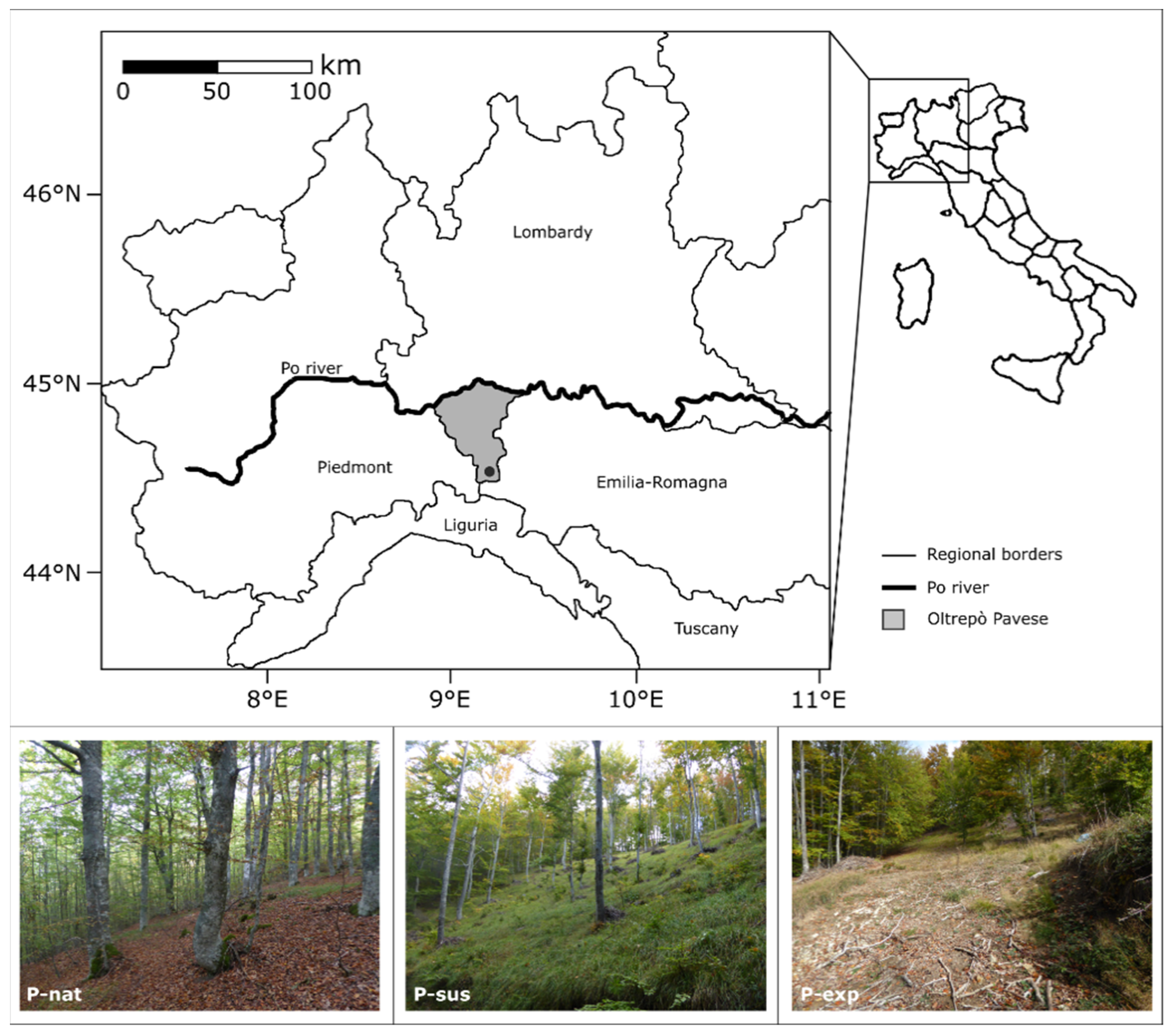
The study area is located in the so-called Oltrepò Pavese, an area in the north-west Italian region of Lombardy, which lies to the south of the Po river (Figure 1). Study sites are located along the northern-facing slope of Mount Terme, at an altitude of 1400 m a.s.l., very close to the “Val Boreca, Monte Lesima” Special Area of Conservation (44°43’ N, 9°15’ E) and to the “Le Torraie-Monte Lesima” Site of Community Importance. Here, beech forests belong to the protected habitat (EU Habitat Directive 92/43, Annex I) named “Asperulo-Fagetum beech forests” (cod. 9130). Mount Terme’s vegetation comprises beech forest and semi-natural dry grasslands and scrubland facies on calcareous substrates.

2.2. Field Sampling

Three plots were identified as representative using remote sensing (Landsat cartography) and field surveys (GPS technology). In particular, three geographic coordinates were randomly selected and used as centroids of three rectangular plots of 500 m² (20 × 25 m) (

Table 1. Main characteristics of the sampled plots.

	P-nat	P-sus	P-exp
Coordinates	44°43’08’’ N, 9°15’30’’ E	44°43’07’’ N, 9°15’31’’ E	44°43’01’’ N, 9°15’32’’ E
Surface (m2)	500
Max altitude (m)	1389	1412	1408
Min altitude (m)	1384	1399	1405
Annual rainfall (mm)	1474
Slope (%)	48	48	46
% Sand in soil	21.2	20.3	20.4
% Silt in soil	48.1	45.9	44.5
% Clay in soil	30.7	33.8	35.1
% Organic matter in soil	4	3.9	3.9

). The three plots have been selected to minimize environmental variability (plots were sampled as close as possible to each other, and are characterized by similar weather conditions and soil characteristics—Table 1), to represent three different management and maintenance conditions. One plot is located in a forest in semi-natural condition (P-nat), a second one in a forest carefully managed to get timber in a sustainable way (P-sus) and a third plot in a forest exploited without management and where trees were totally removed (P-exp). The forest in semi-natural condition (P-nat) is the result of the natural recovery of the forest from a cut made more than twenty years ago. Natural forests do not exist in this territory, which has been managed for hundreds of years. P-sus is a managed forest where timber is harvested cutting down the oldest trees and by maintenance cuts. Both P-sus and P-exp were cut in 2014. The plots have been selected to minimize the differences due to natural conditions (Table 1), in order to represent the effect of human activity (different wood harvesting management) on the whole system’s functioning capacity to store natural capital and provide ecosystem services.

Two sampling campaigns were performed in each plot during summer 2017 and 2018, aiming at counting and measuring trees, shrubs (in understory vegetation) and invertebrates. Trees aboveground and belowground biomass, shrubs and aboveground biomass, invertebrate biomass and the relative annual biomass increase within each plot were accounted. To this purpose, all trees and understory vegetation were measured in each plot together with the deployment of pitfall traps and the extraction of soil cores for the invertebrate collection. The annual increment of biomass, for trees, understory vegetation and invertebrates, was calculated as the difference between the biomass measured in 2017 and the biomass measured in 2018.

2.3. Biomass Estimation

2.3.1. Biomass from Trees

The total aboveground and belowground biomass (trunk, stem, branches, leaves, roots) was estimated using the equations reported in

Table 2. Allometric equations considered in vegetation biomass estimation.

Species		Allometric Equation	Author
Fagus sylvatica	Trunk	Y = 0.0676 × (d)2 + 0.0182 × (d)2 × h	[21]
	Stem (>7 cm)	Y = 0.83 × (d−22.5)2 − 0.0248 × (d-22.5)2 × h
	Stem (from 2 to 7 cm)	Y = 0.0792 × (d)2
	Stem (<2 cm)	Y = 0.093 × (d)2 − 0.00226 × (d)2 × h
	Leaves	Y = 0.0145 × (d)1.9531	[22]
	Roots	Y = 0.106 × (d)2	[23]
Understory	Above-ground biomass	TS = a *Db × Mc	[24]

Y: Biomass (g); d: Diameter at breast height (cm); h: Plant height (m); TS: Aboveground biomass (g/m²); D: Coverage ratio (%); M: Mean aboveground shoot length (cm); a, b, c: Function constants.

.

Standing dead trees were also measured, but their increment was obviously registered as zero.

2.3.2. Biomass from Understory Vegetation

Understory vegetation biomass was reckoned measuring the mean aboveground shoot length and cover of each species.

Understory vegetation in the plots was composed by 62 different species of vascular plants (shrubs and herbaceous plants) and 8 different species of bryophytes. Allometric equations were applied to estimate the biomass in the plots, as reported in Table 2. In particular, the function constants a, b and c are selected according to 13 growth form groups identified by [25]. The species found within the plots, having considerable coverage (greater than 5%), were brought back to the 13 growth form groups and subsequently considered for the biomass estimation.

2.3.3. Net Primary Production

Net Primary Production on a yearly base (NPP) is the net amount of carbon captured by plants through photosynthesis each year [24]. NPP is measured as the quantity of new organic matter that is retained by live plants at the end of a time interval (biomass increase) and the amount of organic matter that was both produced and lost by the plants during the same interval [25].

In this context, NPP was estimated as the annual increase of biomass in trunks, stems and roots, together with the biomass of leaves, Fagus sylvatica being a deciduous species.

2.3.4. Biomass of Invertebrates

In order to sample the invertebrate community, we used two different sampling methods: pitfall traps and soil core extraction. Ground-dwelling invertebrates were sampled with three pitfall traps for each plot. Pitfall traps consisted of a 500 cm³ container, partially filled with a killing/preserving solution [26]. Traps were active for 14 days (October–November 2017). Soil invertebrates, on the other hand, were sampled using a 1000 cm³ soil core (i.e., a soil core measuring 10 × 10 × 10 cm in length, width and height, respectively). Three replicates were realized for each plot. The invertebrates, collected using Berlese–Tullgren extraction funnels traps, were preserved in 90% ethanol. Then, they were sorted and determined at the Order level, while their length was digitally measured using a dissecting microscope and the ImageJ software [27]. The biomass was then estimated using arthropod length measures and following Ganihar’s [28] Taxon-specific equations.

2.4. Soil Erosion Assessment

The quantitative rill-interrill erosion was assessed by means of the Revised Universal Soil Loss Equation (RUSLE) [29,30]. RUSLE is the most common methodology for the assessment of rill and interrill erosion processes and has been widely used for the estimation of soil erosion and to guide development and conservation plans in order to control erosion under different land-cover conditions [31,32]. RUSLE is considered a simple model, since it incorporates data that are easily available and/or accessible, and since it provides reliable results [33]. RUSLE simulates rill and interrill soil erosion considering the effects of soil, topography and land use. The model employs the following expression:

A = R * K * L * S * C * P

(1)

where

A is the mean soil loss per year [Mg ha⁻¹ year⁻¹];

R is the rainfall–runoff erosivity factor [MJ mm ha⁻¹ h⁻¹ year⁻¹];

K is the soil-erodibility factor [Mg h MJ⁻¹ mm⁻¹];

L is the slope–length factor, and S is the slope–steepness factor (dimensionless);

C is the cover-management factor (dimensionless), and

P is the support-practice factor (dimensionless).

To assess and adjust the physical parameters included in the model, a bibliographical survey and basic data collection (including pluviometric, soil, land-use/cover and topographical data) was performed [14].

2.5. Ecosystem Functions Evaluation and Emergy Analysis Application

The general methods for employing emergy synthesis were developed by Odum [12,34]. The concept of emergy synthesis is based on the assumption that the emergy value of a flow (of energy or material) is the sum of all emergy associated to the resources required (directly and indirectly) to create it (

Table 3. Allometric equations considered in vegetation biomass estimation.

Term	Definition
Natural capital	A storage of natural resources of energy, generated and not yet consumed by nature
Ecosystem functions	Ecological processes that control the fluxes of energy and resources through a natural system
Ecosystem service	Tangible or intangible benefits that people derive from ecosystems
Exergy	Exergy is the thermodynamic measure of the maximum work a system can produce under a given environment
Donor-side perspective	A system accounting method representing the value of a resource in terms of the cost of production, in this case accounted as the biosphere’s investment
Emergy	The available energy of one kind (exergy) that is used up in transformations directly and indirectly to make a product or service
Solar emjoule (seJ)	The unit of emergy, a solar equivalent joule. Solar is the most diffuse energy, thus the logical base unit
Unit emergy value (UEV)	The cumulative available energy (emergy) used to create one unit of matter, available energy, information, etc.
Empower	Emergy per unit time
Emergy to money ratio (EMR)	Ratio of emergy supporting an economic system to the currency circulating in the same economic system (units = seJ/€ in this research)
Em-Euro (Em€)	The Euro equivalent of emergy, computed by dividing emergy by the EMR.

).

As a consequence, all inputs to a system must first be determined (emergy input analysis) and then allocated to internal system pathways and exported items (emergy allocation) [35]. Once the fluxes to the system have been identified, it is possible to calculate the solar emergy of each environmental and anthropic (e.g., fuels, human service) input by quantifying either its exergy (i.e., available energy), mass or money value and translating it to solar emergy by means of appropriate unit emergy values (UEV). Unit emergy values are also reckoned as transformities (seJ/J) or specific emergy values (e.g., seJ/g, or emergy per unit money value).

UEVs are calculated on the basis of the total annual emergy inflow to the biosphere from three primary exergy sources of different origins interacting to drive processes within the geobiosphere (the sun, moon and deep-earth heat) that make up the whole annual emergy budget called baseline [36]. The baseline emergy is the reference system for every process, good or service, and the basis of everything physically happening in the biosphere [37,38]. The evaluations we are proposing are based on the 9.26 × 10²⁴ sej/yr baseline [39], and the emergy and transformity values based on different baselines were modified accordingly.

The emergy analysis of Fagus sylvatica forests was developed following the approach proposed by Vassallo [40], which allows us to assess the value of natural capital and of the fluxes that it generates. The former accounting is applied to assess the biophysical value of the stock of resources accumulated in the living structures of the system, whereas the latter is focused on the evaluation of the natural flows supporting the annual biomass production (empower) [41]. These two measures were here considered respectively as the evaluation of natural capital stored and of the ecosystem functions released by the beech stands.

Input items to common beech stands are solar energy, wind, geopotential and the chemical energy of rain, geothermal heat, runoff, transpiration and nutrient consumption (here considered as the C, N and P uptake required from the environment to realize the photosynthesis).

When the total stored emergy (capital) or annual emergy flow (empower) of each plot is calculated, an emergy share can be ascribed to every internal processes occurring in beech forests and to each product or service maintained by the system. The identified forest services are: aboveground biomass increase, roots biomass increase, litterfall generation, understory vegetation biomass increase, invertebrate biomass increase and soil retention.

The solar emergy amount ascribed to each service was determined through the emergy allocation procedures, which include the emergy algebra rules that were sketched in Brown and Herendeen [42] and Odum [12]. According to emergy algebra, the output of a process can be identified as a split or co-product. Splits are represented by flows of the same kind, with different emergy but the same UEV (for example, a water stream that divides into two). Co-products are outflows of a different kind and with different UEV (for example, flows of wool and mutton produced by the sheep agricultural system are co-products). Co-products have different UEVs because they emerge from different stages in the series of transformations during the same process [43].

Since processes on the common beech system provide different products (both from a physical and a functional perspective), they are here considered co-products, meaning that the solar transformity of each service was calculated as the total solar emergy divided by its energy content. Transformity has been proposed as a measure of efficiency when comparing two similar products: a lower transformity of a product reflects the ability to use less past and present work of the biosphere (emergy) to produce a unit of product [16,44].

Once all the internal products or exports are accounted in emergy terms, it is possible to translate these figures into the corresponding monetary value [45]. Emergy is usually translated to money value, expressed in emergy-euros (i.e., em€), by dividing the emergy amount by the average emergy-to-money ratio of an economic system.

3. Results

3.1. Biomass Evaluation

Trees, shrubs, herbaceous vegetation and invertebrate biomass were evaluated, and the results are reported in

Table 4. Trees, shrubs, herbaceous vegetation and invertebrate biomass in the three considered plots.

Compartment	Species/Taxon	Part	P-nat (kg/500 m2)	P-sus (kg/500 m2)	P-exp (kg/500 m2)
Tree	Fagus sylvatica	Trunk	13,219.81	3691.89
		Stem (>7 cm)	1306.02	127.34
		Stem (2 to 7 cm)	2511.08	853.13
		Stem (<2 cm)	1573.18	633.76
		Leaves	398.84	134.81
		Roots	3360.79	1141.81
Total Fagus sylvatica			22,369.71	6582.73
Understory	Rubus hirtus				48.32
	Rubus idaeus			1.80	8.94
	Agrostis capillaris			1.53	39.68
	Brachypodium sylvaticum				7.14
	Carex flacca				7.14
	Cirsium arvense				7.37
	Digitalis lutea			5.22	5.22
	Luzula nivea			8.81
	Poa pratensis				11.19
	Sesleria argentea			77.06	7.14
	Veronica officinalis				0.33
	Fissidens taxifolius			0.26
	Brachythecium glareosum		0.01	0.26
	Pterigynandrum filiforme		0.03	0.31
	Tortula marginata		1.58	1.58	0.15
	Hypnum cupressiforme		1.58	8.28
Total understory			3.21	105.12	142.63
Invertebrates	Acarina	0.16	0.17	0.26
	Araneae		0.01	0.01	0.03
	Opiliones		0.16	0.16	0.16
	Chilopoda/Diplopoda		0.67	1.04	1.16
	Coleoptera larvae		1.46	1.45	2.61
	Collembola		4.56	2.15	3.97
	Hymenoptera		0.05	0.04	0.34
	Anellida		2.48	3.72	1.86
Total invertebrates			9.56	8.75	10.39

.

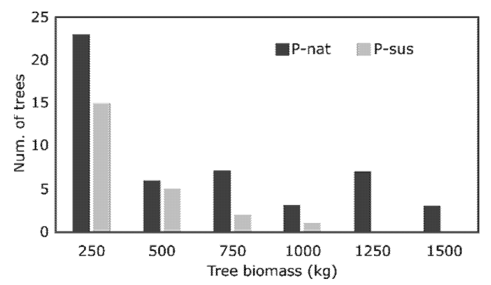
In P-nat (not affected by human activity) 50 trees of F. sylvatica were measured, while in P-sus (recently harvested for timber yield) 46 trees were identified, even if 22 among them showed only shoots from their stumps. Finally, P-exp does not have any tree anymore.

The total tree biomass was found to be 3.4 times higher in P-nat than P-sus. This is due to both the higher number of small size trees in P-nat and the presence of a consistent number of trees with high and very high biomass. In P-sus, on the other hand, the biomass distribution showed a continuous decrease in number of trees with increasing size (Figure 2), never exceeding 1000 kg per tree.

The lack of a consistent tree canopy in P-exp has led the way to a more abundant and complex understory community, which is represented by 11 species in P-exp compared to 10 in P-sus and 4 in P-nat. The total understory biomass copes with the distribution of the number of species with the highest value displayed by P-exp. Extremely low values are displayed by P-nat.

Invertebrate sampling produced a total number of 3160 invertebrates (1087, 888 and 1185 for P-nat, P-sus and P-exp, respectively), belonging to 8 Taxa. A multivariate analysis of similarity revealed no significant differences in the composition of the invertebrate community (ANOSIM; R = −0.007; p = 0.540; 9999 Bootstrap replicates). The Shannon diversity index applied to the invertebrate community (H; 1.44, 1.37 and 1.42 for P-nat, P-sus and P-exp, respectively) is similar in the three plots. Finally, the estimated invertebrates’ biomass was quite similar in the three stands (Table 4).

3.2. Soil Erosion

The application of the RUSLE methodology allowed for the quantification of the rill and interrill erosion in the three plots (

Table 5. Factors and results of the RUSLE methodology.

	Methodology	P-nat	P-sus	P-exp
R factor	[46]	100.44	100.44	100.44
LS factor	[47]	10	6	8
K factor	[30]	0.032799109	0.035214941	0.02083131
C factor	[48]	0.0001	0.0003	0.05
P factor	[49]	1	1	1
RUSLE		0.003294343	0.00636658	0.836918715

).

In the P-nat (not affected by human activity), the loss rate is lower (3.294 kg/ha/year) than in the P-sus recently harvested for timber yield (6.367 kg/ha/year) and in the P-exp that does not have any F. sylvatica trees anymore (83.692 kg/ha/year).

This is due to the different soil and environment characteristics, that make P-exp more subject to erosion than the others in natural condition.

This is also in accord with the general theory revealing that the vegetation protects the soil from erosion [33,50,51,52,53].

3.3. Emergy of Common Beech Stands

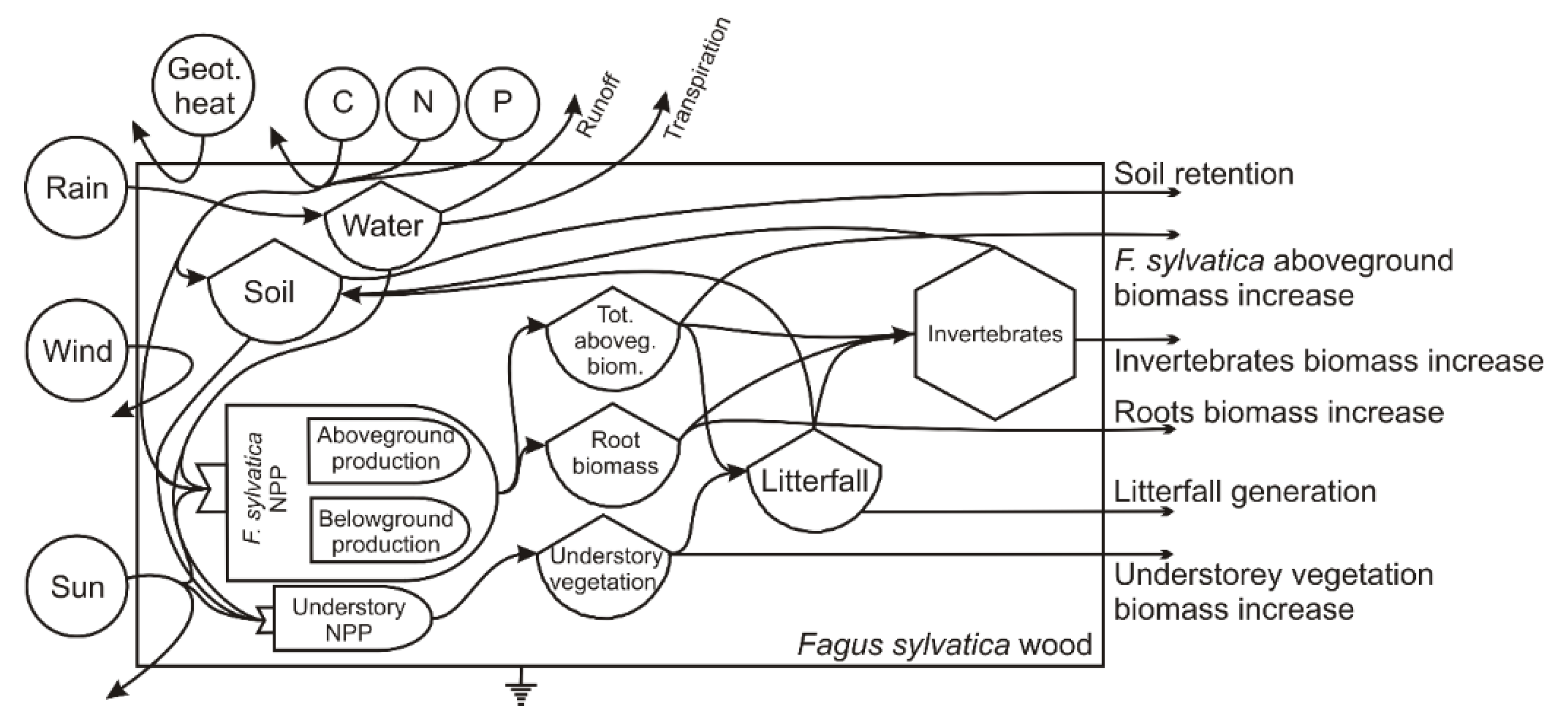
The energy system diagram of a F. sylvatica stand is reported in Figure 3, showing the external sources feeding the system, the internal processes and the provided services. The input of different types of energy (solar radiation, kinetic energy of wind, precipitation and geothermal heat) and resources (nutrients) interacts with the trees, understory and invertebrates biomasses to generate the living structures in the system and to maintain internal cycles such as biomass increase, litter generation and water and soil cycles.

The energy and material flows identified in Figure 3 are also listed in

Table 6. Calculation in emergy units of the flows required in space and time to create the natural capital (items 1–9) stored in the F. sylvatica forests and the emergy required for different system components (items a–e). Equations are reported in Appendix A Table A1.

	Input		Quantity			Unit	UeV	Emergy
			P-nat	P-sus	P-e×p			P-nat	P-sus	P-e×p
1	Sun		1.93 × 1010	9.71 × 109	5.81 × 109	J	1.00 × 100	1.93 × 1010	1.01 × 1010	5.81 × 109
2	Wind		1.53 × 1012	7.70 × 1011	4.61 × 1011	J	2.41 × 103	1.93 × 1015	1.86 × 1015	1.11 × 1015
3	Rain
	3°	Chemical potential	3.88 × 1011	1.96 × 1011	1.17 × 1011	J	2.93 × 104	1.14 × 1016	5.95 × 1015	3.43 × 1015
	3b	Geopotential	2.01 × 1012	1.41 × 1012	1.21 × 1011	J	1.69 × 104	3.39 × 1016	2.48 × 1016	2.04 × 1015
4	Geothermal heat		1.17 × 108	5.88 × 107	3.52 × 107	J	2.00 × 104	2.34 × 1012	1.18 × 1012	1.22 × 1012
5	Runoff		6.05 × 1011	4.26 × 1011	3.65 × 1010	J	2.72 × 104	1.65 × 1016	1.21 × 1016	9.92 × 1014
6	Evapotranspiration		2.18 × 1011	6.72 × 1010	1.41 × 1010	J	2.81 × 104	6.12 × 1015	1.89 × 1015	1.96 × 1015
7	C		1.02 × 107	3.17 × 106	3.12 × 105	g	1.02 × 108	1.04 × 1015	3.25 × 1014	3.19 × 1013
8	N		4.48 × 105	1.61 × 105	5.32 × 104	g	7.40 × 109	3.32 × 1015	1.19 × 1015	3.94 × 1014
9	P		6.09 × 104	2.20 × 104	7.60 × 103	g	2.86 × 1010	1.75 × 1015	6.31 × 1014	2.18 × 1014
	Total emergy							4.34 × 1016	2.80 × 1016	4.22 × 1015
a	Roots biomass							5.81 × 1015	3.05 × 1015	0
b	Aboveground biomass							3.29 × 1016	1.46 × 1016	0
	b.1			Stems				3.22 × 1016	1.42 × 1016	0
	b.2			Leaves				6.89 × 1014	3.60 × 1014	0
C	Understory vegetation							3.98 × 1015	8.47 × 1015	4.78 × 1014
d	Invertebrates							7.31 × 1014	1.94 × 1015	3.74 × 1015

and

Table 7. Calculation in emergy units of the flows exploited on a yearly base (empower) in the F. sylvatica forests. Equations are reported in Appendix A Table A2.

			Annual flow			Unit	UeV	Empower
			P-nat	P-sus	P-e×p			P-nat	P-sus	P-e×p
1	Sun		1.95 × 108	1.95 × 108	1.95 × 108	J	1.00 × 100	1.95 × 108	1.95 × 108	1.95 × 108
2	Wind		1.55 × 1010	1.55 × 1010	1.55 × 1010	J	2.41 × 103	3.73 × 1013	3.73 × 1013	3.73 × 1013
3	Rain
	3°	Chemical	3.93 × 109	3.93 × 109	3.93 × 109	J	2.93 × 104	1.15 × 1014	1.15 × 1014	1.15 × 1014
	3b	Geopotential	2.03 × 1010	2.85 × 1010	2.03 × 109	J	1.69 × 104	3.43 × 1014	4.81 × 1014	3.43 × 1013
4	Geothermal heat		1.18 × 106	1.18 × 106	1.18 × 106	J	2.00 × 104	2.37 × 1010	2.37 × 1010	2.37 × 1010
5	Runoff		6.13 × 109	8.58 × 109	1.23 × 109	J	2.72 × 104	1.67 × 1014	2.33 × 1014	3.33 × 1013
6	Evapotranspiration		2.20 × 109	1.35 × 109	4.74 × 108	J	2.81 × 104	6.19 × 1013	3.80 × 1013	1.33 × 1013
7	C		5.84 × 105	5.05 × 105	2.87 × 105	g	1.02 × 108	5.97 × 1013	5.15 × 1013	2.93 × 1013
8	N		5.23 × 104	4.81 × 104	4.90 × 104	g	7.40 × 109	3.87 × 1014	3.13 × 1014	3.62 × 1014
9	P		6.84 × 103	6.38 × 103	7.00 × 103	g	2.86 × 1010	1.96 × 1014	1.67 × 1014	2.00 × 1014
	Total							7.92 × 1014	8.32 × 1014	4.91 × 1014
a	Roots biomass							1.23 × 1013	1.36 × 1013	0
b	Aboveground biomass							2.33 × 1014	1.18 × 1014	0
	b.1		Stems					1.13 × 1014	6.62 × 1013	0
	b.2		Leaves					1.20 × 1014	5.14 × 1013	0
c	Understory vegetation							0	5.38 × 1012	1.79 × 1013
d	Invertebrates							5.47 × 1014	6.95 × 1014	4.73 × 1014

and translated in emergy equivalents by means of appropriate unit emergy values.

3.3.1. Natural Capital Evaluation

The total stored emergy resulted highest in P-nat and displayed decreasing values when moving to more and more exploited stands. The highest input contributing to stored solar emergy (Table 6) is always due to rain (varying from chemical to geopotential energy in different cases).

The distribution of natural capital among different system components is heterogeneous (Table 6). The highest share of natural capital is stored in the wooden part of the trees (stems), except for P-exp, whose capital is mainly driven by invertebrates that play a major role due to the absence of trees. Over 10% of the total capital is stored belowground in roots in both P-nat and P-sus (Table 6). The understory contribution is especially significant in P-sus, with a 30% share of natural capital.

3.3.2. Ecosystem Functions Evaluation

Total System Functioning

The total empower, given by the resources annually required to maintain the natural capital, is higher in P-sus, while the lowest value is showed again by P-exp. Nitrogen uptake is the highest annual flow in P-nat and P-exp, while P-sus’ annual emergy flow is mainly driven by the geopotential energy of rain (Table 7). In all the considered cases the annual empower is mainly driven by resources conveyed to invertebrates.

Co-Functions Evaluation (Emergy Allocation to Ecosystem Functions)

The solar emergy values of the functions generated by the common beech stands are listed in

Table 8. Ecosystem functions of Fagus sylvatica forests.

P-nat
		Annual Flow	Unit	Transformity (seJ/J)
1	F. sylvatica aboveground biomass increase	7.45 × 109	J	1.06 × 105
	1a-Stem wood	2.96 × 109	J	2.68 × 105
	1b-Stem bark	3.48 × 109	J	2.28 × 105
	1c-Thick branches	6.01 × 108	J	1.32 × 106
	1d-Thin branches	4.02 × 108	J	1.97 × 106
2	roots biomass increase	8.05 × 108	J	9.85 × 105
3	litterfall generation	7.85 × 109	J	1.01 × 105
4	understory vegetation biomass increase	0.00 × 100	J
5	Invertebrate biomass increase	2.94 × 106	J	2.69 × 108
6	soil retention	2.34 × 107	J	3.38 × 107
P-sus
		Annual Flow	Unit	Transformity (seJ/J)
1	F. sylvatica aboveground biomass increase	3.41 × 109	J	2.44 × 105
	1a-Stem wood	2.26 × 109	J	3.69 × 105
	1b-Stem bark	2.41 × 108	J	3.45 × 106
	1c-Thick branches	5.25 × 108	J	1.59 × 106
	1d-Thin branches	3.92 × 108	J	2.12 × 106
2	roots biomass increase	7.02 × 108	J	1.18 × 106
3	litterfall generation	2.65 × 109	J	3.14 × 105
4	understory vegetation biomass increase	4.74 × 107	J	1.76 × 107
5	Invertebrate biomass increase	2.51 × 106	J	3.32 × 108
6	soil retention	2.33 × 107	J	3.56 × 107
P-exp
		Annual Flow	Unit	Transformity (seJ/J)
1	F. sylvatica aboveground biomass increase	0 × 10	J
	1a-Stem wood	0 × 10	J
	1b-Stem bark	0 × 10	J
	1c-Thick branches	0 × 10	J
	1d-Thin branches	0 × 10	J
2	roots biomass increase	0 × 10	J
3	litterfall generation	0 × 10	J
4	understory vegetation biomass increase	3.10 × 108	J	1.58 × 106
5	Invertebrate biomass increase	6.79 × 101	J	7.23 × 1012
6	soil retention	× 100	J

. Here, the transformity of the different functions is calculated according to emergy algebra rules.

In this study, the increase of the aboveground biomass of F. sylvatica, root biomass, litterfall generation, understory vegetation biomass, invertebrate biomass and soil retention were considered co-products, and thus were found to have the same solar emergy but different transformities (Table 8).

The highest solar transformity was displayed by an increase of invertebrate biomass in all the stands considered. Invertebrates’ production and maintenance are extremely expensive in terms of resource flows per unit of energy and require a huge amount of emergy to be produced and kept in the system, despite their low biomass and their limited yearly production.

The stands in natural condition are able to generate wood, root and litterfall in a more efficient way that P-sus, as demonstrated by its lower transformities. Moreover, the soil is more effectively retained in P-nat than in P-sus, if only slightly. On the contrary, the more natural system is unable to generate understory biomass and less efficient in maintaining the invertebrate fauna than the exploited stand. The P-exp plot is then able to provide only a couple of functions (understory vegetation biomass increase and invertebrate biomass increase) but in a very efficient way.

4. Discussion

Wood harvesting is an activity exploiting the provisioning of raw materials from forests to generate economic flows and wealth. Being directly withdrawn from living structures from a complex ecosystem, the wood yield has consequences on the natural stocks and functioning of the forest that are generally neglected or poorly considered when the decision to harvest is made. In this study we applied a donor-based approach to evaluate the effect of wood harvesting on common beech forests. To this purpose, a natural system and two exploited stands, harvested with different levels of invasiveness, were compared to quantify, from a biophysical perspective, the effect of wood harvesting.

The natural stand (P-nat) is able to store the highest natural capital (1.5 times the P-sus and 10.3 times the P-exp), being the one where the wood harvesting is not performed. Here, the understory system is poorly developed, but the trees are higher in number and bigger in size. In fact, the natural capital in P-nat is mainly stored in the tree biomass (89% of the total natural capital), while understory (9% of the total natural capital) and invertebrates (2% of the total natural capital) are less able to stock value in the system.

The same ratio is also shown in the forest harvested in a sustainable way (P-sus), even if a reduced tree coverage, due to the withdrawal of trees, in particular big and mature ones, allows the lower vegetational levels of the forest to obtain more solar radiation. Thus, the diversity and abundance of understory vegetation increases, as revealed by its greater capability to store natural capital (30% of the total natural capital).

The natural capital of the strongly exploited forest (P-exp) has been heavily impacted. The complete removal of the trees from the stand led to (1) a massive natural capital loss and (2) a reversal in the relevance of the forest’s components in terms of the natural capital stored. In P-exp invertebrates store 89% of the total natural capital. The remaining capital of P-exp is associated with understory biomass, which is well established, abundant and diversified due to the lack of mature trees in the plot.

Taking into consideration the ability of the system to annually convey flows and resources, P-nat and P-sus displayed light differences despite evident disparities in natural capital. This is expectedly due to the higher productivity of the trees standing in P-sus that take advantage of the reduced competition and increase the net primary production rate of the system. P-exp displayed again the lowest emergy value, with the trees being absent and the vegetation unable to maintain structures as complex as those of P-nat and P-sus, that call for intense natural fluxes. The total amount of resources yearly exploited is here considered as the biophysical measure of the ecosystem functions provided by the system. Beside the total amount of functions provided, it has been possible to evaluate the efficiency in functions provisioning thanks to the evaluation of the cost per unit of product generated (Table 8). It should not be forgotten that the semi-natural common beech forest (P-nat) is actually the result of a cut of the forest, made more than twenty years ago, and therefore the ecological dynamics within it are more similar to those of P-sus than those that would exist in a hypothetical natural forest that was never cut. In fact, natural forests do not exist in most of Europe’s territory, which has been managed for hundreds of years (natural forest ecosystems account for less than 2% of forests in Western Europe [54,55]). P-nat, where the ecosystem is undisturbed and able to develop toward mature stages, is able to provide, with the maximum efficiency, the entire set of ecosystem functions considered, apart from understory vegetation and an invertebrate biomass increase. These functions which are not directly related to the abundance and biomass of trees in the system are most efficiently generated by P-exp. The reduced tree coverage due to the timber yield let solar radiation reach the lower levels of the forest, increasing the diversity and growth rate of the understory, which is mirrored by the greater efficiency of this compartment. Together with the greater quantity of understory vegetation, an increased ability to maintain a more abundant and productive invertebrate community was assessed, identifying the harvested stands as more able to supply these services when compared to healthier and more mature forests.

Economic Valuation

More and more environmental and resource economists are taking a particular interest in research on forest ecosystem services. Interdisciplinary research involving ecological and economic disciplines is a prerequisite for the more effective management of forest ecosystems [56]. In this context, several authors proposed a number of market and non-market evaluations of the services provided by forests. A list of recent evaluations developed adopting different methodologies is reported in

Table 9. Comparison of forests’ ecosystem services and natural capital estimations. Data have been updated to 2021 values by power of the dollar over time (U.S. Labor Department’s Bureau of Labor Statistics).

Authors	Methods	System	Minimum	Maximum
Annual Services
Merlo and Croitoru [57]	non-market evaluations	Italian forests	403		$/ha/year
Croitoru [58]		Mediterranean forest	74	263
Bernetti et al. [59]		Protected Italian forests	3306
Costanza et al. [60]		World’s forests	311	18,375
Campbell and Brown [61]	emergy	US national forests	158		em$/ha/year
Campbell and Tilley [2]		Maryland forest	302	824
Turcato et al. [16]		Italian Pinewood	9576	12,096
This study		Italian beechwood	19,000	32,000
Stored Capital
Campbell and Brown [62]	emergy	US national forests	361,920		em$/ha
This study		Italian beechwood	166,000	1,700,000

.

The range of values is wide both because of the different methodologies adopted and the variety of services and functions provided by forests. Among the studies reported in Table 9, several studies estimated forests’ value based on users’ perception of the supplied services. Recently, an increasing number of economists are advocating biophysical measurements as a basis for valuation [62]. Despite being useful to get a valuation of the user’s perception of nature’s value, these measures are intrinsically affected by the comprehension of the system, by preferences and by the contingencies of the market [63]. Nonetheless, ecosystem functions neglected or poorly evaluated by humans and market may play a key role in ecosystem functioning and the provisioning of other services useful and valuable to mankind [64]. As a consequence, the total value of a system (and of a forest, in the specific case) cannot disregard an assessment based on a biophysical accounting based on the amount of resources invested by nature to maintain the system, independently of the presence of direct users and the value they ascribe to a generated service [45]. Emergy analysis allows us to obtain this evaluation adopting a donor-based perspective and ascribing the cost of directly and indirectly exploited resources. Moreover, with a donor-based biophysical evaluation, it is possible to estimate the value of the natural capital stored in a system and of generated functions alike [40].

The natural capital stored in common beechwoods, according to the evaluation performed in this work, drops abruptly in the case of timber harvesting. The monetary equivalent of the capital stored in wood in natural condition (P-nat) amounts to 1.7 million Em€ ha⁻¹, decreasing to 1.1 million Em€ ha⁻¹ in the case of wood harvested in a sustainable way (P-sus) and falling to 166,000 Em€ ha⁻¹ when the wood is completely exploited for timber production (P-exp). By the way, forest cutting, in the face of a decrease in natural capital, causes an increase in terms of both plant and animal diversity. In our analysis this is represented by the highest value of annual flows in P-sus. In a management perspective, this has to be interpreted as an operation of capital liquidation to increase the gains. Even according to market rules, financial capital liquidation presents a certain level of risk, and it is unrealistic to foresee that a continuous liquidation or the bankrupt is inevitable. Borrowing this framework from the economy, the same concept is applicable (mutatis mutandis) to the management of a natural system. Natural capital is subjected to a range of human pressures (e.g., climate change, desertification) representing threats to its maintenance. Eroding natural capital is always a risk, since in a precautionary approach, to maintain services provisioning at the current level, natural capital must be kept intact [40,64]. As a consequence, the loss should at least be carefully accounted and possibly balanced by an increase in functionality, otherwise the system is likely to be compromised (like in P-exp). If markets are not ruled and managed in an ecologically sustainable way, they will tend to over-produce market goods and services, erode natural capital and under-produce ecosystem functions [65]. An ecological system of valuation is thus necessary because human assessments do not measure the real contributions of natural ecosystems to human well-being [66].

Emergy analysis was applied to the identification of six different functions provided by F. sylvatica forests. All the services were here considered co-products of the common beech wood system maintained by all the inputs listed in Table 7. As a consequence of the application of emergy algebra’s rules, the total emergy of the entire system is assigned to each service. As a consequence, P-nat functions are worth 31,135 Em€ ha⁻¹ year⁻¹ and P-sus 32,688 Em€ ha⁻¹ year⁻¹, while P-exp services amounted to 19,293 Em€ ha⁻¹ year⁻¹. The timber harvesting activity does not provoke ecosystem services provision loss when performed in a sustainable way. However, if the forest is strongly exploited, the estimated loss amounts to 13,391 Em€ ha⁻¹ year⁻¹. This difference might be interpreted as the loss of value due to a backward shift on the succession of a beechwood after timber harvesting, and it is the final consequence of the reduction in complexity of the system.

5. Conclusions

This work was developed seeking to assess the variations of natural capital and ecosystem services provisioning due to different levels of exploitation of beech woods. To this aim, three plots, assumed to be differentiated primarily by the level of exploitation, were analyzed. The accounting system was based on a biophysical, donor-based perspective providing a valuation not affected by human preferences (i.e., emergy analysis). Emergy is an accounting method able to evaluate the work of the biosphere in terms of direct and indirect solar energy converging to support the production of products and services [14]. According to this method, the more work of the biosphere is embodied in generating natural resources and ecosystem services, the greater their value. Emergy provides an alternative measure of the value of natural capital and ecosystem services, assessing their cost of production in terms of the biophysical flows used to supp their generation and use [66,67,68,69]. The donor-based perspective, offered by emergy-based approaches, gives a promising alternative to the challenging issue of the assessment of natural value generally based on the stated preferences of people (either by means of the market price or contingent valuation processes) [70].

We found that the system in semi-natural condition (P-nat) is able to store the highest natural capital and to provide ecosystem functions with the highest efficiency. The sustainable exploitation of the forest to harvest wood has negative consequences in terms of the natural capital stored in the system but sets off a rise of the energy flowing in the system expectedly focused on the natural capital recovery. A complete exploitation of a beech forest, on the contrary, leads to the depletion of natural capital and to a decrease in the capacity of the system to convey and exploit resources, making the system unable to provide several services.

Starting from the promising findings of this research, further investigations may be necessary to account for the variability within the forest types, to improve the accounting system including other compartments to the system (e.g., microbial community, fungi, vertebrates) and to take into consideration the time variability. Forests, in fact, are dynamic systems expected to evolve toward more complex structures and to recover form disturbance. In this context, a time cross-sectional study may confirm the hypothesis of the backward shift on the succession of forests after timber harvesting and shed light on the recovery process.

Despite its limitation, this research is a step toward developing a methodology that can be used to inform policies for the mutual benefit of humanity and the environment, aiming at bringing environmental accounting to the decision and management process.

References

- Krieger, D.J. The Economic Value of Forest Ecosystem Services: A Review; The Wilderness Society: Washington, DC, USA, 2001. [Google Scholar]
- Campbell, E.T.; Tilley, D.R. Valuing ecosystem services from Maryland forests using environmental accounting. Ecosyst. Serv. 2014, 7, 141–151. [Google Scholar] [CrossRef]
- Tsiantikoudis, S.; Zafeiriou, E.; Kyriakopoulos, G.; Arabatzis, G. Revising the environmental Kuznets curve for deforestation: An empirical study for Bulgaria. Sustainability 2019, 11, 4364. [Google Scholar] [CrossRef] [Green Version]
- Yu, X.; Ma, S.; Cheng, K.; Kyriakopoulos, G.L. An evaluation system for sustainable urban space development based in green urbanism principles-a case study based on the Qin-Ba mountain area in China. Sustainability 2020, 12, 5703. [Google Scholar] [CrossRef]
- Kimmins, J.P. From science to stewardship: Harnessing forest ecology in the service of society. For. Ecol. Manag. 2008, 256, 1625–1635. [Google Scholar] [CrossRef]
- Mendoza, G.A.; Prabhu, R. Multiple criteria decision making approaches to assessing forest sustainability using criteria and indicators: A case study. For. Ecol. Manag. 2000, 131, 107–126. [Google Scholar] [CrossRef]
- Kyriakopoulos, G.L.; Kolovos, K.G.; Chalikias, M.S. Woodfuels prosperity towards a more sustainable energy production. Commun. Comput. Inf. Sci. 2010, 112, 19–25. [Google Scholar] [CrossRef]
- Kyriakopoulos, G.L.; Chalikias, M.S.; Kalaitzidou, O.; Skordoulis, M.; Drosos, D. Environmental viewpoint of fuelwood management. CEUR Workshop Proc. 2015, 1498, 416–425. [Google Scholar]
- Millennium Ecosystem Assessment. Ecosystems and Human Wellbeing: Current State and Trends; Island Press: Washington, DC, USA, 2005. [Google Scholar]
- Franzese, P.P.; Buonocore, E.; Paoli, C.; Massa, F.; Stefano, D.; Fanciulli, G.; Miccio, A.; Mollica, E.; Navone, A.; Russo, G.F.; et al. Environmental accounting in marine protected areas: The EAMPA project. J. Environ. Account. Manag. 2015, 3, 323–331. [Google Scholar] [CrossRef]
- Odum, H.T. Self organization, transformity and information. Science 1988, 242, 1132–1139. [Google Scholar] [CrossRef] [Green Version]
- Odum, H.T. Environmental Accounting: Emergy and Environmental Decision Making; John Wiley and Sons: New York, NY, USA, 1996; 384p. [Google Scholar]
- Costanza, R.; d’Arge, R.; de Groot, R.; Farber, S.; Grasso, M.; Hannon, B.; Limburg, K.; Naeem, S.; O’neill, R.V.; Paruelo, J.; et al. The value of the world’s ecosystem services and natural capital. Nature 1997, 387, 253–260. [Google Scholar] [CrossRef]
- Turcato, C.; Paoli, C.; Scopesi, C.; Montagnani, C.; Mariotti, M.G.; Vassallo, P. Matsucoccus bast scale in Pinus pinaster forests: A comparison of two systemsby means of emergy analysis. J. Clean. Prod. 2015, 96, 539–548. [Google Scholar] [CrossRef]
- Cowling, R.M.; Egoh, B.; Knight, A.T.; O’Farrell, P.J.; Reyers, B.; Rouget, M.; Roux, D.; Welz, A.; Wilhelm-Rechman, A. An operational model for mainstreaming ecosystem services for implementation. Proc. Natl. Acad. Sci. USA 2008, 105, 9483–9488. [Google Scholar] [CrossRef] [PubMed] [Green Version]
- Vassallo, P.; Paoli, C.; Tilley, D.R.; Fabiano, M. Energy and resource basis of an Italian coastal resort region integrated using emergy synthesis. J. Environ. Manag. 2009, 91, 277–289. [Google Scholar] [CrossRef] [PubMed]
- Masiero, M.; Pettenella, D.; Secco, L. From failure to value: Economic valuation for a selected set of products and services from Mediterranean forests. For. Syst. 2016, 25, 11. [Google Scholar] [CrossRef] [Green Version]
- Bateman, I.J.; Carson, R.T.; Day, B.; Hanemann, M.; Hanley, N.; Hett, T.; Jones-Lee, M.; Loomes, G.; Mourato, S.; Pearce, D.W. Economic Valuation with Stated PreferenceTechniques: A Manual, UK Department of Transport; Edward Elgar Publishing Inc.: Cheltenham, UK, 2002. [Google Scholar]
- Maes, J.; Egoh, B.; Willemen, L.; Liquete, C.; Vihervaara, P.; Schägner, J.P.; Grizzetti, B.; Drakou, E.G.; la Notte, A.; Zulian, G.; et al. Mapping ecosystem services for policy support and decision making in the European Union. Ecosyst. Serv. 2012, 1, 31–39. [Google Scholar] [CrossRef]
- TEEB. The Economics of Ecosystems and Biodiversity: Mainstreaming the Economics of Nature: A Synthesis of the Approach, Conclusions and Recommendations of TEEB; The Economics of Ecosystems & Biodiversity: Geneva, Swizerland, 2010. [Google Scholar]
- Ruiz-Peinado, R.; Montero, G.; del Rio, M. Biomass models to estimate carbon stocks for hardwood tree species. For. Syst. 2012, 21, 42–52. [Google Scholar] [CrossRef]
- Santa Regina, I.; Tarazona, T.; Calvo, R. Aboveground biomass in a beech forest and a Scots pine plantation in the Sierra de la Demanda area of northern Spain. Ann. Sci. For. 1997, 54, 261–269. [Google Scholar] [CrossRef] [Green Version]
- Melillo, J.M.; McGuire, A.D.; Kicklighter, D.W.; Moore, B., III; Vorosmartyt, C.J.; Schlosst, A.L. Global climate change and terrestrial net primary production. Nature 1993, 363, 234–240. [Google Scholar] [CrossRef]
- Clark, D.A.; Brown, S.; Kicklighter, D.W.; Chambers, J.Q.; Thomlinson, J.R.; Ni, J.; Holland, E.A. Net primary production in tropical forests: An evaluation and synthesis of existing field data. Ecol. Appl. 2001, 11, 371–384. [Google Scholar] [CrossRef]
- Bolte, A. Biomasse und Elementvorräte der Bodenvegetation auf Flächen des Forstlichen Umweltmonitorings in Rheinland-Pfalz (BZE 2010, Level II); Universität Göttingen: Göttingen, Gemany, 2006; 45p. [Google Scholar]
- Woodcock, B.A. Insect Sampling in Forest Ecosystems; Pitfall trapping in ecological studies; Leather, S.R., Ed.; Blackwell Science: Oxford, UK, 2005; pp. 37–57. [Google Scholar]
- Rueden, C.T.; Schindelin, J.; Hiner, M.C.; DeZonia, B.E.; Walter, A.E.; Arena, E.T.; Eliceiri, K.W. ImageJ2: ImageJ for the next generation of scientific image data. BMC Bioinform. 2017, 18, 529. [Google Scholar] [CrossRef]
- Ganihar, S.R. Biomass estimates of terrestrial arthropods based on body length. J. Biosci. 1997, 22, 219–224. [Google Scholar] [CrossRef]
- Renard, K.G.; Foster, G.R.; Weesies, G.A.; McCool, D.K.; Yoder, D.C. Predicting Soil Erosion by Water: A Guide to Conservation Planning with the Revised Universal Soil Loss Equation (RUSLE); Handbook No. 703.; US Department of Agriculture: Washington, DC, USA, 1997; 404p.
- Wischmeier, W.H.; Smith, D.D. Predicting rainfall erosion losses d a guide to conservation planning. In Agriculture Handbook No. 537; US Department of Agriculture Science and Education Administration: Washington, DC, USA, 1978; p. 163. [Google Scholar]
- Mati, B.M.; Veihe, A. Application of the USLE in a savannah environment: Comparative experiences from East and West Africa Singapore. J. Trop. Geogr. 2001, 22, 138–155. [Google Scholar] [CrossRef]
- Angima, S.D.; Stott, D.E.; O’Neill, M.K.; Ong, C.K.; Weesies, G.A. Soil erosion prediction using RUSLE for central Kenyan highland conditions. Agric. Ecosyst. Environ. 2003, 97, x295–x308. [Google Scholar] [CrossRef]
- Morgan, R.P.C. Soil Erosion and Conservation; Longman: Essex, UK, 1986; p. 298. [Google Scholar]
- Odum, H.T. Handbook of Emergy Evaluation Folio #2: Emergy of Global Processes. Center for Environmental Policy; University of Florida: Gainesville, FL, USA, 2000; p. 30. [Google Scholar]
- Tilley, D.R.; Swank, W.T. EMERGY-based environmental systems assessment of a multi-purpose temperate mixed-forest watershed of the southern Appalachian mountains, USA. J. Environ. Manag. 2003, 69, 213–227. [Google Scholar] [CrossRef] [PubMed]
- Brown, M.T.; Campbell, D.E.; Ulgiati, S.; Franzese, P.P. The geobiosphere emergy baseline: A synthesis. Ecol. Model. 2016, 339, 89–91. [Google Scholar] [CrossRef]
- Brown, M.T.; Ulgiati, S. Updated evaluation of exergy and emergy driving the geobiosphere: A review and refinement of the emergy baseline. Ecol. Model. 2010, 221, 2501–2508. [Google Scholar] [CrossRef]
- Vassallo, P.; Paoli, C.; Fabiano, M. Emergy required for the complete treatment of municipal wastewater. Ecol. Eng. 2009, 35, 687–694. [Google Scholar] [CrossRef]
- Campbell, D.E. A revised solar transformity for tidal energy received by the earth and dissipated globally: Implications for emergy analysis. In Emergy Synthesis: Theory and Applications of the Emergy Methodology, Proceedings of the 1st Biennial Emergy Analysis Research Conference, Gainesville, FL, USA, 2–4 September 1999; Brown, M.T., Ed.; Center for Environmental Policy, Department of Environmental Engineering Sciences, University of Florida: Gainesville, FL, USA, 2000; pp. 255–264. [Google Scholar]
- Vassallo, P.; Paoli, C.; Buonocore, E.; Franzese, P.P.; Russo, G.F.; Povero, P. Assessing the value of natural capital in marine protected areas: A biophysical and trophodynamic environmental accounting model. Ecol. Model. 2017, 355, 12–17. [Google Scholar] [CrossRef]
- Paoli, C.; Povero, P.; Burgos, E.; Dapueto, G.; Fanciulli, G.; Massa, F.; Scarpellini, P.; Vassallo, P. Natural capital and environmental flows assessment in marine protected areas: The case study of Liguria region (NW Mediterranean Sea). Ecol. Model. 2018, 368, 121–135. [Google Scholar] [CrossRef]
- Brown, M.T.; Herendeen, R.A. Embodied energy analysis and EMERGY analysis: A comparative view. Ecol. Econ. 1996, 19, 219–235. [Google Scholar] [CrossRef]
- De La Fuente, G.; Asnaghi, V.; Chiantore, M.; Thrush, S.; Povero, P.; Vassallo, P.; Petrillo, M.; Paoli, C. The effect of Cystoseira canopy on the value of midlittoral habitats in NW Mediterranean, an emergy assessment. Ecol. Model. 2019, 404, 1–11. [Google Scholar] [CrossRef]
- Vassallo, P.; Bastianoni, S.; Beiso, I.; Ridolfi, R.; Fabiano, M. Emergy analysis for the environmental sustainability of an inshore fish farming system. Ecol. Indic. 2007, 7, 290–298. [Google Scholar] [CrossRef]
- Pulselli, F.M.; Coscieme, L.; Bastianoni, S. Ecosystem services as a counterpart of emergy flows to ecosystems. Ecol. Model. 2011, 222, 2924–2928. [Google Scholar] [CrossRef]
- Angeli, L.; Bottai, L.; Costantini, R.; Ferrari, R.; Gardin, L.; Innocenti, L.; Maerker, M.; Siciliano, G. Sviluppo di metodologie di analisi per lo studio dell’erosione del suolo in ambienti mediterranei: Applicazione specifica a un’area pilota. In Proceedings of the Atti Della VIII Conferenza nazionale ASITAI, Rome, Italy, 14–17 December 2004; Volume 1, pp. 87–92. [Google Scholar]
- Moore, I.D.; Wilson, J.P. Lengtheslope factors for the revised universal soil loss equation: Implified method of estimation. J. Soil Water Conserv. 1992, 47, 423–428. [Google Scholar]
- Panagos, P.; Borrelli, P.; Meusburger, K.; Alewell, C.; Lugato, E.; Montanarella, L. Estimating the soil Erosion cover-management factor at the European scale. Land Use Policy 2015, 48, 38–50. [Google Scholar] [CrossRef]
- Rellini, I.; Scopesi, C.; Olivari, S.; Firpo, M.; Maerker, M. Assessment of soil erosion risk in a typical Mediterranean environment using a high-resolution RUSLE approach (Portofino promontory, NW-Italy). J. Maps 2019, 15, 356–362. [Google Scholar] [CrossRef]
- Wischmeier, V.H. Cropping-management factor evaluations for a universal soil-loss equation. Soil. Sci. Soc. Am. 1960, 24, 322–326. [Google Scholar] [CrossRef]
- Elwell, H.A.; Stocking, M.A. Vegetal cover to estimate soil erosion hazard in Rhodesia. Geoderma 1976, 15, 61–70. [Google Scholar] [CrossRef]
- Francis, C.F.; Thornes, J.B. Runoff hydrographs from three Mediterranean vegetation cover types. In Vegetation and Erosion-Processes and Environments; Thornes, J.B., Ed.; John Wiley: Hoboken, NJ, USA, 1990. [Google Scholar]
- Alias, L.J.; Lopez-Bermudez, F.; Marin-Sanleandro, P.; Romero-Diaz, M.A.; Martinez, J. Clay minerals and soil fertility loss on Peric Calcisol under a semiarid Mediterranean environment. Soil Technol. 1997, 10, 9–19. [Google Scholar] [CrossRef]
- WWF. 1998. Available online: http:/www.wwf.es (accessed on 25 February 2021).
- Forest Europe, 2020: State of Europe’s Forests 2020. Available online: https://foresteurope.org/wp-content/uploads/2016/08/SoEF_2020.pdf (accessed on 5 March 2021).
- Garcia, S.; Abildtrup, J.; Stenger, A. How does economic research contribute to the management of forest ecosystem services? Ann. For. Sci. 2018, 75, 53. [Google Scholar] [CrossRef] [Green Version]
- Merlo, M.; Croitoru, L. Valuing Mediterranean Forests. Towards Total Economic Value; CABI Publishing: Wallingford, UK, 2005; p. 406. [Google Scholar]
- Croitoru, L. How much are Mediterranean forests worth? For. Policy Econ. 2007, 9, 536–545. [Google Scholar] [CrossRef]
- Bernetti, I.; Alampi Sottini, V.; Marinelli, N.; Marone, E.; Menghini, S.; Riccioli, F.; Sacchelli, S.; Marinelli, A. Quantification of the total economic value of forest systems: Spatial analysis application to the region of Tuscany (Italy). Aestimum 2013, 62, 29–65. [Google Scholar]
- Costanza, R.; de Groot, R.; Sutton, P.; van der Ploeg, S.; Anderson, S.J.; Kubiszewski, I.; Farber, S.; Turner, R.K. Changes in the global value of ecosystem services. Glob. Environ. Change 2014, 26, 152–158. [Google Scholar] [CrossRef]
- Campbell, E.T.; Brown, M. Environmental accounting of natural capital and ecosystem services for the US National Forest System. Environ. Dev. Sustain. 2012, 14. [Google Scholar] [CrossRef]
- De Groot, R.S.; Fisher, B.; Christie, M.; Aronson, J.; Braat, L.; Haines-Young, R.; Gowdy, J.; Maltby, E.; Neuville, A.; Polasky, S.; et al. Integrating the Ecological and Economic Dimensions in Biodiversity and Ecosystem Service Valuation; The Economics of Ecosystems and Biodiversity (TEEB), Ecological and Economic Foundations: Geneva, Switzerland, 2010. [Google Scholar]
- Bingham, G.; Bishop, R.; Brody, M.; Bromley, D.; Clark, E.; Cooper, W.; Costanza, R.; Hale, T.; Hayden, G.; Kellert, S.; et al. Issues in ecosystem valuation: Improving information for decision making. Ecol. Econ. 1995, 14, 73–90. [Google Scholar] [CrossRef]
- Vassallo, P.; Paoli, C.; Rovere, A.; Montefalcone, M.; Morri, C.; Bianchi, C.N. The value of the seagrass Posidonia oceanica: A natural capital assessment. Mar. Pollut. Bull. 2013, 75, 157–167. [Google Scholar] [CrossRef] [PubMed]
- Antle, J.; Stoorvogel, J.J. Predicting the Supply of Ecosystem Services from Agriculture. Am. J. Agric. Econ. 2006, 88, 1174–1180. [Google Scholar] [CrossRef]
- Odum, H.; Odum, E. The Energetic Basis for Valuation of Ecosystem Services. Ecosystems 2000, 3, 321–323. [Google Scholar] [CrossRef]
- Paoli, C.; Gastaudo, I.; Vassallo, P. The environmental cost to restore beach ecoservices. Ecol. Eng. 2013, 52, 182–190. [Google Scholar] [CrossRef]
- Paoli, C.; Vassallo, P.; Dapueto, G.; Fanciulli, G.; Massa, F.; Venturini, S.; Povero, P. The economic revenues and the emergy costs of cruise tourism. J. Clean. Prod. 2017, 166, 1462–1478. [Google Scholar] [CrossRef]
- Vassallo, P.; Beiso, I.; Bastianoni, S.; Fabiano, M. Dynamic emergy evaluation of a fish farm rearing process. J. Environ. Manag. 2009, 90, 2699–2708. [Google Scholar] [CrossRef] [PubMed]
- Raffaelli, D.; White, P.C.L. Chapter One—Ecosystems and Their Services in a Changing World: An Ecological Perspective. In Advances in Ecological Research; Woodward, G., O’Gorman, E.J., Eds.; Academic Press: Cambridge, MA, USA, 2013; Volume 48, pp. 1–70. [Google Scholar]