
Sustainable Supply Chain Decisions under E-Commerce Platform Marketplace with Competition


1
School of Business, Changshu Institute of Technology, Suzhou 215500, China
2
Southern Jiangsu Economic and Social Development Research Center, Changshu Institute of Technology, Suzhou 215500, China
3
Department of Literature Service, Jiangsu Information Institute of Science & Technology, Nanjing 210042, China
4
Economics and Management School, Nantong University, Nantong 226019, China
*
Author to whom correspondence should be addressed.
Sustainability 2021, 13(8), 4162; https://doi.org/10.3390/su13084162
Submission received: 11 March 2021
/
Revised: 31 March 2021
/
Accepted: 6 April 2021
/
Published: 8 April 2021
(This article belongs to the Special Issue New Trends in Sustainable Supply Chain and Logistics Management)
Abstract
:Motivated by the industrial observation that the e-commerce platform marketplaces (e.g., Amazon) are increasingly launching sustainable strategies, this study aims to build an analytical framework to guide managers on making sustainable decisions. This study builds a stylized game-theoretical model in the sustainable supply chain context, where the competitive traditional product manufacturers sell their products through the platform’s marketplace, while the platform decides whether to introduce the green products and the pricing strategy. We find that, when the evaluation difference for the green product is sufficiently low, the introduction of the green product by the platform benefits the manufacturers (or third-party sellers). Interestingly, a higher platform fee makes a higher likelihood of a win-win situation between the platform and manufacturers. Moreover, when consumers value green products sufficiently higher than traditional products, the traditional products’ manufacturers can also benefit from the green product entry.
1. Introduction
1.1. Motivation of Industrial Observation
E-commerce platforms are gradually attaching importance to the introduction and sale of green or environment-friendly products. It is reported that Amazon has launched an “eco-friendly” shopping platform in the UK and other European countries to sell household products with sustainable credentials. Moreover, a new green e-commerce platform VEO launched in June of 2019 in the UK, even calling itself “Earth-friendly Amazon”. Wal-Mart, one of the largest retailers that turn to operate as a platform-based enterprise, is a typical example to embed suitability strategies in their business strategy [1]. Wal-Mart has increased its investment in products’ energy-saving performance, improving 25% efficiency of products with the energy-intensive initiative [2]. At the policymaker level, the Chinese government even openly advocates e-commerce platforms to fulfill their green responsibilities and develop and launch more green products. For the environment aspect, consumers choose more green products can also promote the development of environmental protection. It is therefore urgent for the platforms to facilitate green products with eco-friendly characteristics.
To cater to the trend of sustainable development, the platform has started to introduce green products. However, this green strategy is bound to conflict with the existing third-party sellers or manufacturers on the platform. Fundamental differently with the traditional retailing mode, under which the manufacturers first wholesale the products to retailers. Then the retailers sell them to consumers at a retail price, and the manufacturers determine retail prices and pay a fraction of revenue to the platform under this model. Under this new emerging mode, the classic double marginalization effect is eliminated, which often plays critical roles in much supply chain literature (e.g., Huang et al. [3] and Lou et al. [4]). Instead, the platform fee for the manufacturers charged by the platform plays a new role in shaping manufacturers’ pricing behaviors for the on-sales products, most of which are traditional products. On the one hand, the extent of the platform fee decides how much revenue the manufacturers save for themselves; on the other hand, it also affects the platform’s gains between from the manufacturers and from the green products. Moreover, the competition among manufacturers also affects whether the platform introduces the green products considering its overall profitability. Therefore, the Platform-led supply chain has raised a series of new questions different from the traditional supply chain management [5]. In the specific context of this study, we focus on the pricing strategy of the platform and competitive manufacturers as well as the effects of green product involvement.
1.2. Motivation of Literature Background
A retrieve of the previous work on green product strategy in a supply chain context shows no prior studies examining the pricing strategy of the green product with both impacts of platform selling mode and upstream competition among traditional product manufacturers. In this study, we adopt an extended Hotelling model, which is taken as a spatial location model, to study the horizontal differentiation between competing firms. In the literature, the Hotelling model was first applied to characterize two firms competing within a linear city. Salop [6] presents a variant of Hotelling’s model (known as the circular spatial market model). In addition to the circular model, Zhang and Zheng [7] incorporate a line of fixed length to represent consumers’ heterogeneous preferences for certain product characteristics, which in turn forms a cylinder model. Biscaia and Mota [8] provide a critical review of models based on spatial competition. The spatial model can easily capture consumers’ preferences on firm’s location. We extend the Hotelling model by adding a divergent line to capture consumers’ heterogeneous preferences over green product characteristics. We remark that a similar version of this model was studied by Chen and Riordan [9], but their focus is on the product variety of multiple manufacturers. In our model, each line represents a consumer segment and their preferred products, thus it appropriately depicts the sales and competition of green products on the platform, which is the phenomenon that this study tries to investigate.
Moreover, most of the previous work on green product strategy focus on greenness level decisions of the manufacturer (e.g., Guo et al. [10], Heydari et al. [11], Hong and Guo [1]), this study focuses on the pricing strategy of the green product in the platform-selling background. Furthermore, most of the green product models always assume that the consumers are willing to pay more for the green product compared with the traditional products. However, in reality, given that a green product has the same cost as a traditional product, this means that a green product may need to invest some of the budgets that would otherwise be devoted to developing the product’s functional properties into green properties. This means that consumers may not always be willing to value green products more than traditional products. In our model, we consider both situations that the consumers’ valuation for green product may be lower or higher than the traditional products.
1.3. Research Questions
Motivated by the industrial observations and literature, the research of this study is to address the following natural questions:
- Should the platform introduce the green product to compete with traditional product manufacturers who are selling products on its marketplace?
- Will the green product introduced by the platform hurt the existing manufacturers?
- How does the platform selling mode as well as competition among existing manufacturers affect firms’ price decisions?
The aim of this study is to explore the strategies of the platform’s pricing strategy with the involvement of green product, and the manufacturers’ strategies to cope with green product entry. Our study helps to shed light on why the platforms are willing to introduce more and more green products, and clarifies the key drivers of firms’ pricing strategies facing green product entry. Combined with the current commercial trend of the platform economy and the economic motivation of green product sales, this study also tries to bring some managerial insights for enterprises’ green decision-making.
1.4. Key Findings
Our analysis yields several key findings. First, when the evaluation difference for the green product is sufficiently low, green product’s entry benefits the traditional product manufacturers. The platform always benefits from the introduction of the green product. This implies that manufacturers need not always worry about the product cannibalization issue caused by the green product entry. The key driver of this win-win situation is that the green product absorbs less loyal consumers for traditional products so that all firms can focus on their loyal consumers. At the same time, the competition among manufacturers could be mitigated as well. The threshold of valuation difference also depends on the magnitude of platform fee as well as the consumers’ attitudes to the green product. Second, a higher platform fee makes a higher likelihood of a win-win situation between the platform and manufacturers. In the recent retailing world, platforms such as Amazon and JD.com are more and more monopolistic, and the manufacturers will be worse off if the platforms raise platform fees. To take the case without green product as a baseline, a green product may more likely increase the manufacturers’ profits. Last, as the platform introduces a high-valued green product, the manufacturers can even benefit from the green product entry when the valuation difference for the green product is high enough. In this circumstance, the green product takes some less loyal customers of traditional products, which in turn makes the manufacturers focus more on their loyal customers and also obtain more profits.
1.5. Research Methodology and Structure
We employ a stylized game-theoretical model to examine the impacts of a low-valued green product, which captures the features of a typical platform supply chain with a platform and competitive manufacturers. The model is based on the Hotelling model [12], and also we extend it to mimic the featured marketplace in the context of this study. Furthermore, our model can also help to examine the impacts of a high-valued green product under the same settings.
The remainder of this study is organized as follows. Section 2 reviews the relevant literature. Section 3 setups the model’s framework by employing an extended Hotelling model. Section 4 analyzes the benchmark without green product entry. Section 5 analyzes the case with green product entry and obtains related insights about the impacts of the green product. In Section 6, we extend the basic model by considering a high-valued green product. Section 7 concludes this study and discusses the limitations which provide some directions for future research. All proofs are provided in the Appendix A.
2. Literature Review
Our focus is on how green product introduction and traditional product competition affect firms’ price decisions in the platform supply chain. For brevity, we limit our review to literature related to green product introduction, platform supply chain, and online product competition. In what follows, we review the extant research in these areas and highlight the contributions of our work.
In the context of green product introduction decisions, some studies investigated the impacts of green product’ positioning and pricing problems. For example, Hong et al. [13] examine a green product competes with an existing traditional product in a manufacturer-retailer supply chain, and they find that consumers’ reference behaviors significantly influence the green product’s positioning and pricing strategies. Agi and Yan [14] investigate the impact of the supply chain’s power structures on the pricing strategies of a newly introduced green product against with existing traditional product. The authors find that a manufacturer-led structure is better than a retailer-led structure to launch the green product. By simultaneously considering consumer environmental awareness and non-green (regular) product reference, Hong et al. [15] investigate a green-product pricing problem, and the authors reveal that the green product’s pricing strategy is significantly affected by asymmetric information. Wang et al. [16] investigate the influence of inter-supply-chain competition on the wholesale price, and the green degree of the green supply chain members, and their results indicate that the inter-supply-chain competition has a negative correlation with the wholesale price of green product. Meng et al. [17] explore products collaborative pricing policies in a dual-channel green supply chain; the authors find that government subsidies can cause lower price but higher demand for green products; furthermore, government subsidies also make the manufacturer better off, while the retailer’s profit depends on the number of government subsidies. Chen and Sheu [18] examine a company’s green product entry decisions by considering the effect of market uncertainty and consumer rationality. Nielsen et al. [19] examine the optimal pricing and investment decision of green product for two competing green supply chains, and they explore that the strategic integration decision with rivals at the horizontal level or with partners at the vertical level have any effect on green product types. Unlike traditional competitive analysis of non-green products, differentiation may not always be the best choice for society, and the authors show that the non-differentiation for the green product is favorable. Jamali and Rasti-Barzoki [20] investigate the pricing and greenness decisions of the green product in competition with the non-green product. In their model, the market consists of two dual-channel supply chains, including retail and internet channels, while the green product distributed solely by one supply chain, and their analysis yields that the centralized scenario cause achieves a high green degree comparing with the decentralized scenario. Unlike previous research, this study focuses on the pricing strategy of the green product in the platform-selling background. Our study is close to Xu [21], who also uses a game-theoretical model to study the interactions between an entrant and an incumbent in an e-commerce marketplace; however, their model incorporates neither the effect of competition among incumbents nor the impact of a green product. Besides, to the maximum of our knowledge, our model first examines the impact of traditional product competition on green product introduction as well as pricing decisions.
With the rise of the platform economy in recent years, the platform selling model gradually causes a boom in academic research. A similar selling model, as a store-within-a-store which is normally adopted in department stores, is firstly examined by Jerath and Zhang [22]. Under an online retailing setting, Abhishek et al. [23] investigate whether and when the e-tailers should use a platform selling model or and conventional reselling model. Similarly, Tian et al. [24] investigate a dominant e-tailer’s platform selling decisions for competitive upstream suppliers. Both above studies specify the strategic role of platform selling in eliminating the double marginalization effect, which always occurs under the conventional reselling model. Cao et al. [25] examine the dilemma faced by firms who sell new and remanufactured products offline that need to consider whether to enter e-commerce platforms considering that more and more consumers are shopping online on e-commerce platforms rather than shopping offline. Yan et al. [26] investigate whether and when the manufacturer should introduce the platform selling in addition to the reselling channel, they also study these problems by incorporating online spillover. Zhang and Zhang [27] examine the e-tailer’s demand information sharing strategy with the manufacturer who may operate brick-and-mortar stores offline, they also compare the impacts of two prevailing retailing including agency selling and reselling. Wei et al. [28] investigate two competitive e-tailers’ selling format choices (reselling or agency selling) for the common manufacturer’s products on their online platforms, and they also model the effects of e-tailers’ referral fees and the difference in e-tailers’ market shares. In the context of the hotel industry, Liao et al. [29] and Ye et al. [30] study the different strategic effects between reselling and agency selling in a monopolistic and competitive environment, respectively. Fan et al. [31] examine the value of this horizontal cooperation behavior in an e-commerce platform setting, and they find that horizontal cooperation can foster channel coordination. Bai et al. [32] investigate how government subsidies affect pricing and service quality strategies under different online recycling channel structures that include an e-commerce platform. The authors find that manufacturers gain a competitive advantage from subsidies by offering higher recycling prices, which forces the platform to raise recycling prices as well. Unlike previous studies, this study examines the impacts of the platform selling model on the decisions of green products in the platform supply chain. The green products introduction is becoming an emerging trend in the e-commerce platform retail environment, but it has rarely been mentioned in previous studies.
Related to our study, several studies focus on the effects of competition in the online supply chain mode. Ba et al. [33] investigate several e-tailers compete on price as well as the positioning of their quality offerings through a general vertical differentiation model in an oligopolistic setting. They find that the adverse price effect still holds in a more general setting. Ding et al. [34] investigate service competition in an online duopoly market, and the duopoly retailers compete in both price and service time. As an increasing trend of Omni-channel retailers that operate physical and online channels, Jin et al. [35] investigate the retailers’ strategic decisions on the adoption of the cross-channel return policies from in a duopoly setting, they find that the adoption of the buy-online-return-to-physical store policy by one or both retailers can occur in equilibrium if the retailers are sufficiently differentiated. In a more general setting, Fan et al. [36] examine two competitive e-tailers’ physical store mode decisions, that is, to launch physical stores for showing only (as a showroom) or for actual transactions (as a selling store). They find that an asymmetric channel configuration occurs in equilibrium when the proportion of the store consumer segment is not too high. In the contexts of symmetric information and asymmetric information, Cao et al. [37] respectively explore a retailer’s optimal return strategy offline and whether or not to enter a platform. Differing from above studies, this study builds an extended the traditional Hotelling model, and expands a line segment of the original model into three lines. In our model, each line represents a consumer segment and their preferred products, thus it perfectly depicts the sales and competition of green products on the online platform.
3. The Model
Consider a platform supply chain where two symmetric manufacturers (M1 and M2) enroll in an E-commerce platform (E) and sell directly to consumers. The manufacturer M1 (M2) sells product T1 (T2) in E’s marketplace at the expense of paying a commission fee. We assume that Product T1 and T2 are horizontally differentiated traditional products without green characteristics. E has the option to sell a green product (G) in its own self-run store, which is also horizontally differentiated from extant traditional products. This assumption is reasonable because the platforms such as Amazon usually have uncanny ability to tap consumer data and position the green products rightly. For example, Amazon recently launched a new program to help customers discover and shop for sustainable products [38].
3.1. Firms
As shown in Figure 1, we model the featured marketplace using an extended Hotelling model [12]. Each of the products competing in the market offers one variety. To simplify the presentation of our analysis and clarify the key drivers for our main insights, the per-unit production costs for all products are assumed to be equal to , where is a constant and normalized to zero. Thus, the green product G owns more eco-friendly characteristics but may have less functional performance, since the traditional products can invest more in functional research and development than the green products under the same budget. The traditional products and green product indexed , are located at three ends of the triple Hotelling line as shown in Figure 1., respectively. Following Kuksov and Lin [39], Rhee and Thomadsen [40], and Jing [41], we assume consumers derive a base value from the product , where is a constant that represents basic utility to all consumers when the product meets the minimum quality standard . In other words, captures the reservation value of a consumer who does not need more than a basic product of minimal quality. defines the product quality and valuation where is a scale factor that reflects consumers’ attitudes to green products. We let for traditional products while for green products in the basic model. It captures that the valuation of the green product for the consumer is lower than the traditional product under the same cost. We will relax this assumption in Section 6 to assume .
3.2. Consumers
As shown in Figure 1, we assume a unit mass of consumers is uniformly distributed on the Hotelling lines. Each of the lines starts from the midpoint (center) with unit length, in our model, three lines of one-half length form a local market segment for each product. Each line (denoted as ) terminates at the center and originates at the other end. Consumers preferring product are distributed on line and called as product ’s local consumers. Denote the consumer on line at a distance from the origin by (, ), where , where
If this consumer buys the local product , she will derive the (indirect) utility , where is the consumers’ strength of preference to product characteristics and is the price of the product . Instead, if the consumer chooses to buy another product , she must travel a distance of () because the distance between any two products is equal to 1. Hence, the (indirect) utility derived from the nonlocal product will be . The marginal consumer who is indifferent between the two products, i.e., , is at a distance from product .
When making a purchase decision, it is intuitive that consumers can easily find all products set by the search engine of e-platform. Hence, unlike the literature on the Hotelling model assumes that consumers consider at most two products in one line, our model allows a consumer to any other lines in addition to the local line in which she resides. Particularly, when E does not introduce product G, all consumers in line (, ) will choose traditional products (T1 or T2) that offer a lower price. When both traditional products have an identical price, we assume that consumers randomly choose one of them. Furthermore, we assume that is relatively high so that the market is fully covered; that is, each consumer will buy one product from the marketplace. Our consumer choice model captures consumers’ differences in attitude between traditional and green products. Meanwhile, it also captures the competition that exists in the marketplace already.
3.3. Game Sequences
We model the interaction among the M1, M2, and E as a Stackelberg game. We treat the platform proportional fee as exogenously determined. This platform fee is the same for all products within a certain category, but it differs across product categories. Even so, it is observed that this platform fee rate is stable from year to year. Empirical data indicates that Amazon’s charging platform fee ranges from 6% to 25% of the sale price depending on the product category, while JD.com’s platform fee for most product categories ranges from 5% to 12% [24].
The sequence of events is as follows: E, as the Stackelberg-game leader, decides whether to introduce G. Then, both M1 and M2 simultaneously determining retail prices and for the products T1 and T2, respectively; if G entry, E also sets the retail price as well. Finally, for a given set of retail prices for all products, consumers make purchasing decisions.
4. The Benchmark Case without Green Product
When E does not introduce G (indexed by the superscript “(0)”), each consumer can buy a traditional product from either M1 or M2. For consumers in (, ), provided the marginal consumer who is indifferent between the products T1 and T2 (i.e., ), and . If , then customers in will choose T2 products; the other consumers in will buy the product T1. The same situation also applies to consumers in line (, ). For consumers in line (, ), as mentioned in Section 3.2, all of them will buy the traditional products that offer a lower price; while those consumers will buy the traditional products from either T1 or T2 randomly with 1/2 probability as both manufacturers offer the same prices for their products.
First, we consider the symmetrical case that both manufacturers offer the same prices for their products, that is, . Both manufacturers’ demands are and . Per the sequence of events as stated in Section 3.3, we use backward induction to solve the game among the E, M1, and M2. In this case, both manufacturers simultaneously set the retail price to maximize their profits as follows, respectively:
To jointly solve the above maximization problems per first-order conditions, it yields the equilibrium retail prices with profits and . Then, we consider the asymmetrical case that both manufacturers offer different prices for their respective products, without loss of generality, we assume . We can show that the NBMs have no motivation to deviate the symmetrical equilibrium unilaterally. Please see the proof in the Appendix A.
5. Analysis of The Case with Green Product
With the introduction of the green product by the platform, as stated in Section 3.2, there exist two cases per the pricing of each product.
5.1. Case (1):
In this case, E sets a relatively low price so that all consumers in line (, ) will buy their preferred product G. By contrast, some consumers who are adjacent to the end of the line (, ) will also buy product G. Thus, the marginal consumer who is indifferent between the traditional products and green product (i.e., ) locates at the line (, ). That is, . Thus, for the consumers in line (, ), those with will buy the product , while those with will buy product G. All the consumer in line (, ) will buy their preferred product G. Therefore, in this case, the product G’s demand and product ’s demand are presented as follows:
The firms’ profit functions are and , where . We use backward induction to solve the equilibrium solution in this case, the results of this analysis are presented in the lemma below.
Lemma 1.
In Case (1), there is a unique set of solutions for the firms’ optimal prices and profits: (i) if, such that,,,,, and; (ii) if, such that,,,,.
One can quickly obtain from Lemma 1 that the green product obtains a higher demand than a separate traditional product when the valuation difference for the green product between traditional products and green product (i.e., ), that is, ; otherwise, each product obtains equal demand. In this case, E prices aggressively for product G, the market demand is jointly shaped by pricing and the valuation difference for the green product among various products, which in turn determines the intensity of competition among all products.
5.2. Case (2): or ,
In this case, E sets a relatively high price so that a part of product G’s local consumers who are adjacent to the end of the line (, ) will buy from the manufacturer(s) who offered a lower price. Especially when both manufacturers offer the same prices (), we assume the product G’s local consumers who are likely to buy traditional products will randomly choose a product with a probability . More specifically, provided the marginal consumer who is indifferent between the product and G (i.e., , ), and , the consumer in line (, ) will buy the product G if ; and the other consumers will choose the traditional products that offered a lower price, or randomly buy a product from either M1 or M2 with profitability when both manufacturers offer an identical price.
Specifically, when one manufacturer offers a lower price than the other one, the manufacturer who offered a lower price will take all of those customers. Without loss of generality, we let . Thus, all consumers in will choose the product T1 only if , while each manufacturer acquires half of the consumers in . For the market segmentation between two manufacturers, provided the marginal consumer who is indifferent between the products T1 and T2 (i.e., ), and , the consumer in line (, ) will buy the product T1 if ; the other customers in of the line (, ) will choose the product T2. Hence, we can obtain the demands , , and for the products T1, T2, and G as below:
The firms’ profit functions are and , where . Depending on the relation between prices of both traditional products, that is, and , the firms face two formulations of the demand function. Next, we use backward induction to solve the equilibrium solution, the results of this analysis are presented in the lemma below.
Lemma 2.
In Case (2), there is a unique set of solutions for the firms’ optimal prices and profits: (i) if, such that,,,,, and; (ii) if, such that,,,, and.
Similar to Lemma 1, the market demand also depends on both pricing and the valuation difference for the green product between traditional and green products. In case (i), E sets the price of product G less aggressively, the relatively high price makes the product G obtains less demand than the traditional products when the valuation difference for the green product is relatively high. In case (ii), the outcome is equal with the case (ii) in Lemma 2; that is, each of the products takes up the full of its local market. Therefore, the pricing strategy is at a moderate level. To compare the outcomes stated in Lemma 1 and Lemma 2, and then find out firms’ optimal strategies under the case with green products. To summarize the above outcomes and we obtain Proposition 1 as follows.
Proposition 1.
(i) Case (1). For intermediate valuation difference for the green product (), the unique equilibrium isand. (ii) Case (2). For low valuation difference for the green product (), the unique equilibrium isand; for low valuation difference for the green product () or high valuation difference for the green product (), the unique equilibrium isand; where,,, andare presented in the Appendix A.
Proposition 1 shows that E sets the price of product G less aggressively only when the valuation difference for the green product is sufficiently low or high. When the valuation difference for the green product is sufficiently low, E sets product G’s price such that all products equally share the market. When the valuation difference for the green product is sufficiently high, E sets a higher price for product G, which results in losing some market share. This is because an intensive competition urges E to focus on the local consumers of product G. By doing so, E can obtain a higher profit margin in the price of losing some market share. When the valuation difference for the green product is at an intermediate level, E gets more aggressive on product G’s pricing so that all products obtain equal market shares. Due to the valuation disadvantage of product G, E will never poach the local consumers of traditional products, no matter how low the platform fee is. This is because E also acquires profit by earning a proportion of manufacturers’ revenue, thus the lower price of product G caused by the competition may also hurt E itself. Next, given the results in the benchmark case, we can obtain the following Proposition by comparing the profits of each firm in all parameter regions stated in Proposition 1.
Proposition 2.
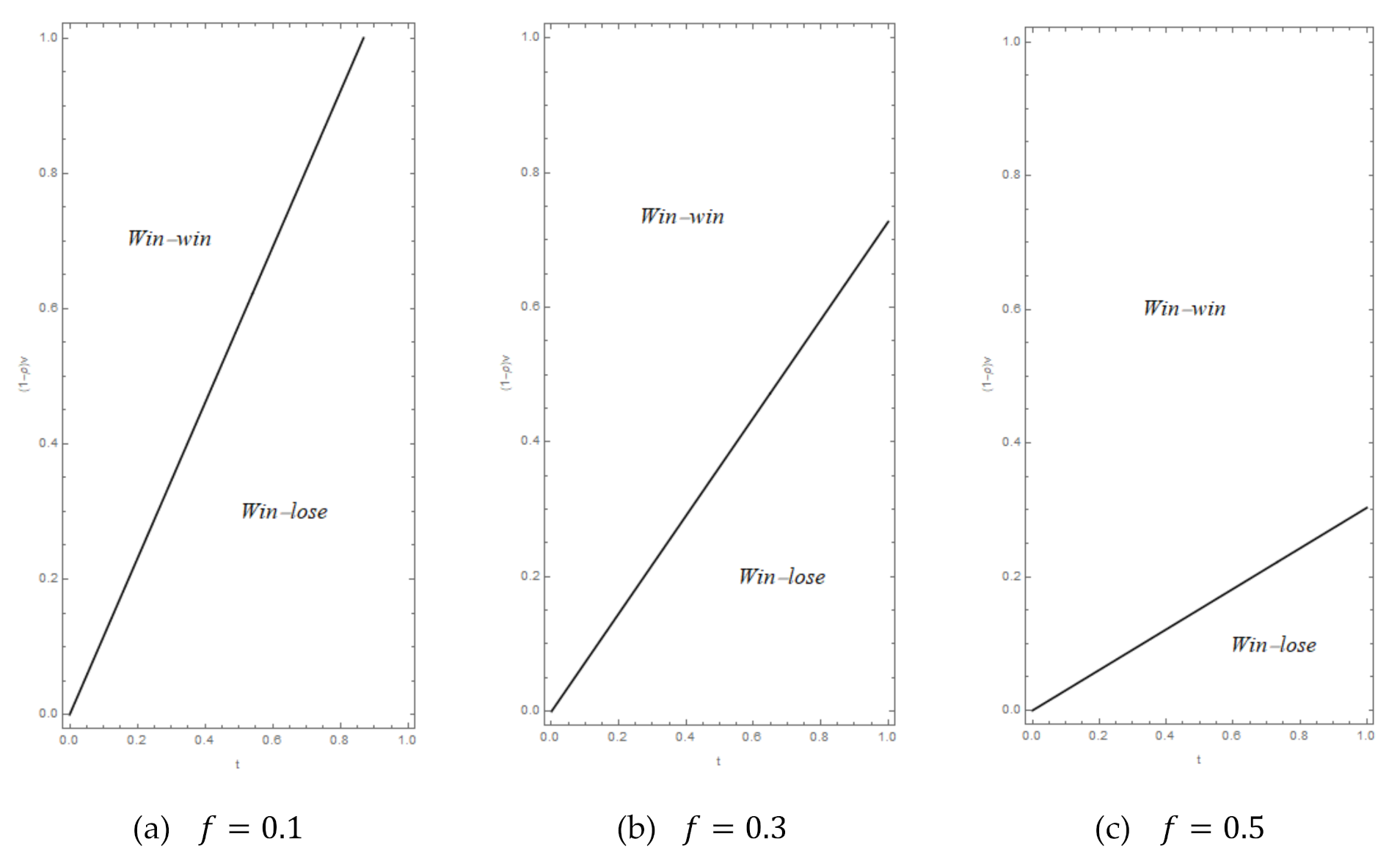
When the valuation difference for the green product is relatively low (), a win-win situation occurs, that is, both the manufacturers and platform are better off with green product introduction; otherwise, a win-lose situation occurs, that is, the platform is better off while manufacturers are worse off. An increase in platform fee expands the win-win parameter region.
Proposition 2 shows that the platform always benefits from selling the green product. While the manufacturers benefit from the green product’s entry when the valuation difference for the green product is sufficiently low. As shown in Figure 2, the marginal consumer in the benchmark case locates at the right end of product G’s local consumers. After the introduction of product G, the location of the marginal consumer may move to the center of lines (for Case (1) or (2)) or a certain point in the line of product G. The above change of market segmentation indicates that manufacturers lose much market share with the product G entry, thus they lose profits in most circumstances. However, when the valuation difference for the green product is low enough, the manufacturers can benefit from product G’s entry since they can focus on their local consumers by charging a higher price; meanwhile, they need not set a low price to absorb product G’s local consumers. As a result, the manufacturers can obtain higher profit margins, which exceed the loss of market shares. For the platform, the introduction of product G enhances its pricing power, and makes more profit through the new product with controllable product cannibalization. Interestingly, as stated in Proposition 2 and shown in Figure 3, a higher platform fee makes a broader parameter region for a win-win situation. This is because the high platform fee enhances the power of E, the manufacturers get worse off in the benchmark case and thus get more benefit.
6. The Case of High Evaluation for the Green Product by Consumers ()
In this section, we will examine the impacts of a high evaluation for green product by consumers (). Following the same procedure in the basic model, we can derive the equilibrium outcome in the following Proposition.
Proposition 3.
(i) Case (1). For sufficiently low evaluation difference for the green product (), the unique equilibrium is and ; for sufficiently high evaluation difference for the green product (), the unique equilibrium is and . (ii) Case (2). For relatively low evaluation difference for the green product (), the unique equilibrium is and ; for relatively high evaluation difference for the green product (), the unique equilibrium is and ; where .
Proposition 3 shows contrast results compared to the main model. Namely, either a high or a low evaluation difference for green product induces the platform’s aggressive pricing, while an intermediate evaluation difference for the green product makes the platform prices less aggressive. As aforementioned, E faces a trade-off between revenue sharing from manufacturers and profit gain from product G. In this case, under an intermediate evaluation difference (or competition), E benefits from the traditional products more than from the green product, hence it is more suitable for E to maintain a moderate pricing strategy for product G. Moreover, under a high evaluation difference (or competition), E benefits from the product G more than from the traditional products; meanwhile, under a low evaluation difference (or competition), All of E, M1, and M2 can resort to a higher profit margin from the local consumers. Thus, E prices aggressively for product G under both the above situations. Next, given the results in the benchmark case, we can obtain the following Proposition by comparing the profits of each firm in all parameter regions in Proposition 3.
Proposition 4.
When the evaluation difference for the green product is either sufficiently low () or sufficiently high (), a win-win situation occurs, that is, both the platform and manufacturers are better off with green product entry; otherwise, a win-lose situation occurs, that is, the platform is better off while manufacturers are worse off.
Proposition 4 shows that the results presented in Proposition 3 still hold, that is, all of E, M1, and M2 get better off with a product G entry when the evaluation difference is sufficiently low. However, with a high evaluation for the green product by consumers, such a win-win situation can also occur when the evaluation difference is high enough. This is because the high-valued product G absorbs the consumers around the center of lines, and the manufacturers can abstract more surplus from the local consumers since the weak competition with the product G. As a result, the manufacturers gain more profit from their loyal consumers who exceed the loss of market shares of swing consumers. The reason for this phenomenon does not occur in the case of low-valued product G is that, the low-valued product G cannot bring more profit for E to offset the loss of traditional products under similar situations.
7. Discussion and Conclusions
Our model focuses on the green product related decisions in the context of the platform supply chain, where consists of an e-commerce platform (e.g., Amazon, JD.com, Taobao.com) and two competitive manufacturers. In our model, the manufacturers are dedicating to selling traditional products in the platform’s marketplace, while the platform can introduce a green product through its self-run store. Our study helps to shed light on why the platforms are willing to introduce more and more green products, and clarifies the key drivers of firms’ pricing strategies facing green product entry.
Our analysis yields several findings and insights as follows: (i) the introduction of the green product by the platform can either intensify or soften the price competition between traditional product manufacturers, and (ii) the platform fee reshapes the pricing strategy of green product, which lead to several counterintuitive results:
First, the competition in the e-commerce marketplace may have a positive impact on existing manufacturers. Specifically, as the evaluation difference for the green product is at a sufficiently low level, the introduction of the green product by the platform benefits the manufacturers. This implies that the green product not only benefits the environment but also benefits the market. A low evaluation difference for a green product often indicates a fierce market competition, and the green product may mitigate the competition among exiting manufacturers; the managers of manufacturers or third-party sellers should adjust their pricing strategy based on the pricing strategy of the green product as well as the magnitude of a platform fee set by the platform.
Second, a higher platform fee of an e-commerce marketplace can make a higher likelihood of a win-win situation for all parties. In the recent retailing world, platforms such as Amazon and JD.com are more and more monopolistic, and the manufacturers will be worse off if the platforms raise platform fees. To take without green product as a baseline, a green product may not result in product cannibalization; in contrast, it is more likely to increase the existing sellers’ profits. Through our analysis, the introduction of green products can improve the profits of existing manufacturers on the platform for two reasons; On the one hand, the introduction of green products can attract fluctuating customers in the market, so that manufacturers can focus more on loyal customers and claim more consumer surplus. On the other hand, the platform maintains a certain platform fee, which is conducive to obtaining the sales profit of green products and preventing the manufacturers from leaving the marketplace.
Last, in the case of a high evaluation for the green product by consumers, the manufacturers can even benefit from green product introduction when the evaluation difference for the green product is high enough. In this circumstance, the high-valued green product takes some less loyal customers of traditional products, which in turn makes the manufacturers focus more on their loyal customers and also obtain more profits. The extension of the model further verifies the robustness of the conclusion in this paper. The difference is that in the expansion model, green products attract more swing-type consumers because of higher valuation. However, when product differentiation is large enough, existing manufacturers can still benefit; Of course, platforms still benefits from the introduction of green product.
We conclude the study by pointing out the limitations of this study and some directions for future work. First, our model extended the classic Hotelling model consists of a line with two ends. For simplicity, we add two lines and two ends to the original line, while have not put more lines for the traditional or green products. Even so, our main results should be qualitatively the same as more lines are introduced. Since our stylized model captures the competition and simplicity between traditional products. However, considering multiple green products may yield more insights, since the competition among the green products could affect the decisions of both the platform and traditional product manufacturers. Second, to focus on the horizontal competition among all products, our model treats the qualities or consumer valuations as exogenously determined. Although the quality decisions of manufacturers are more strategic (long-term) than the pricing decisions (short-term), and abundant vertically differentiated firms are innately asymmetric and broadly exist in reality [42], to extend our model to let the qualities be endogenously determined may yield more insights for the green product entry in the context of e-commerce platforms. Last, extensions of our model that may be of interest would be to capture other factors, such as asymmetric information, bounded rational behavior, and platform competition. We expect that, as this study preliminarily explores the effects of the trend of e-commerce platforms introducing more and more green products, many other related research topics will be studied to extend our understanding of the effects of green products in the context of e-commerce platforms.
Author Contributions
Conceptualization, J.W.; methodology, J.W. and Z.W.; investigation, J.W. and X.G.; writing—original draft preparation, J.W.; writing—J.W. and X.G. All authors have read and agreed to the published version of the manuscript.
Funding
None.
Institutional Review Board Statement
Not applicable.
Informed Consent Statement
Not applicable.
Data Availability Statement
Not applicable.
Conflicts of Interest
The authors declare no conflict of interest.
Appendix A
Appendix A.1. Proof of Section 4
We consider the asymmetrical case that both manufacturers offer different prices for their respective products, without loss of generality, we assume . In other words, we investigate whether the manufacturers have the motivation to deviate the symmetrical equilibrium unilaterally. In this case, all consumers in spoke (, ) will buy product T1. Thus, the demands are and . Both manufacturers solve the maximization problems as follows, respectively:
Subject to
We firstly solve M1’s problem, given , which leads to the response functions (i) if and (ii) if , that is, this case degenerates to the symmetrical case. Then, we solve M2’s problem leading to (i) if and (ii) if , that is, this case degenerates to the symmetrical case. By combining the above cases, it yields that and should sustain simultaneously, which leads to and ; under which the constraints of and can never be satisfied, hence there is no asymmetrical equilibrium exists. That is, both manufacturers will not deviate from symmetrical equilibrium.
Appendix A.2. Proof of Lemma 1
In this case, the platform sets a relatively low price so that all consumers in line (, ) will buy their preferred green product. By contrast, some consumers who are adjacent to the center in line (, ) will also buy the green product. Thus, the marginal consumer who is indifferent between the products and G (i.e., ) locates at the line (, ). That is, . Thus, for the consumers in line (, ), those with will buy the product , while those with will buy the product G. All the consumer in line (, ) will buy their preferred product G. Therefore, in this case, the demand for green product and traditional product are as shown as Equations (1) and (2) respectively. The firms’ profit functions are and , where . Next, we use backward induction to solve the equilibrium solution in this case. In the second stage of the game, the firms solve the profit maximization problems as below:
Subject to:
Notice that in this case consumers in (, ) will consider products and G only, hence each manufacturer will solve her profit maximization problem separately and simultaneously, while all consumers in (, ) will consider product G only. Without loss of generality, we firstly solve M1 and platform’s problems with respect to and as below:
Subject to:
For ’s maximization problem, the first-order condition of yields . requires . Hence, we can obtain (1.a) if , and (1.b) If .
For ’s maximization problem, the first-order condition of yields ; requires . Hence, we can obtain (2.a) if , and (2.b) If . So, we have four possible combinations to consider. (1) Combination 1: Scenario (1.a) v.s. (2.a). By jointly solving and , we have ; both and requires . (2) Combination 2: Scenario (1.a) v.s. (2.b). By jointly solving and , we have and ; always sustains, while requires . (3) Combination 3: Scenario (1.b) v.s. (2.a). By jointly solving and , we have and ; requires , while always sustains. (4) Combination 4: Scenario (1.b) v.s. (2.b). In this combination, since both solutions are corner solution, it is clear that it dominated by the above respective case under all possible range of . So, this combination is infeasible. Per the property of symmetricity, we can obtain the same solution for M2 and E, so, for each combination above, we can obtain (i) and if ; (ii) and if ; and (iii) and if . When , for the above solution (ii), we have and ; for the above solution (iii), we have we have and . One can quickly obtain that and under , thus solution (iii) is not available.
Appendix A.3. Proof of Lemma 2
In this case, the demands , , and are represented by Equations (3)–(5), respectively. The firms’ profit functions are and , where . Depending on the relation between prices of products T1 and T2, that is, and , the firms face two formulations of the demand function. Next, we use backward induction to solve the equilibrium solution case by case. First, we use backward induction to seek the symmetrical equilibrium. In the second stage of the game, the firms solve the profit maximization problems as below:
Subject to:
Notice that in this case consumers in line (, ) will consider product only, while consumers in line (, ) will consider both products G and . Hence each manufacturer will solve her profit maximization problem separately and simultaneously. Without loss of generality, we firstly solve M1 and E’s problems with respect to and as below:
Subject to:
For ’s maximization problem, the first-order condition of yields . requires . Hence, we can obtain (1.a) if ; and (1.b) If . For ’s maximization problem, the first-order condition of yields ; requires . Hence, we can obtain (2.a) if , and (2.b) If . So, we have four possible combinations to consider: (1) Combination 1: Scenario (1.a) v.s. (2.a). By jointly solving and , we have and ; both and requires . (2) Combination 2: Scenario (1.a) v.s. (2.b). By jointly solving and , we have and ; always sustains, and requires . (3) Combination 3: Scenario (1.b) v.s. (2.a). By jointly solving and , we have and ; requires , and always sustains. (4) Combination 4: Scenario (1.b) v.s. (2.b). In this combination, since both solutions are corner solution, it is clear that it dominated by the above respective case under all possible range of . So, This combination is infeasible.
Per the property of symmetricity, we can obtain the same solution for M2 and E, so, for each combination above, we can obtain (i) and if ; (ii) and if ; and (iii) and if . When , for the above solution (ii), we have and ; for the above solution (iii), we have we have and . One can easily obtain that and under , thus solution (ii) is not available.
Next, we check the case of Asymmetrical pricing (, ). In this case, without loss of generality, we let . Notice that in this case consumers in line (, ) will consider product only, those in line (, ) will consider both and , those in line (, ) will consider products G and .
Subject to:
By looking into , one can see that is independent in ; the first-order condition of yields which always holds for M2. We then solve M1 and E’s problems with respect to and as below. For ’s maximization problem, the first-order condition of yields . requires . Hence, we can obtain (1.a) if , and (1.b) If . For ’s maximization problem, the first-order condition of yields . requires . Hence, we can obtain (2.a) if , and (2.b) If . Since always holds, we first consider all combinations for and as below: (1) Combination 1: Scenario (1.a) v.s. (2.a). By jointly solving and , we have and ; both and require . (2) Combination 2: Scenario (1.a) v.s. (2.b). By jointly solving and , we have and ; always sustains, and requires . (3) Combination 3: Scenario (1.b) v.s. (2.a). By jointly solving and , we have and ; requires , and always sustains. (4) Combination 4: Scenario (1.b) v.s. (2.b). In this combination, since both solutions are corner solution, it is clear that it dominated by the above respective case under all possible range of . So, this combination is infeasible.
Plugging in each combination, we can obtain: (i) ; always sustains, and requires ; (ii) , can never sustain, thus this solution is infeasible; and (iii) , can never sustain, thus this solution is infeasible. When , for the above solution (i), we have and .
To compare M2’s solutions in the above symmetrical pricing case as below: (1) If , then . Since and under , we obtain . (2) If , then . Since , thus we obtain . In summary, M2 owns no incentive to increase the retail price, hence the asymmetrical pricing case is infeasible.
Appendix A.4. Proof of Proposition 1
Since under support , the following analysis has three cases. (1) When , we have . Since holds, we thus obtain . Furthermore, we have . Since holds, we thus obtain . Therefore, in this case, all firms prefer Case (2). (2) When , we have and . Since , we thus obtain and . Therefore, in this case, all firms prefer Case (2). (3) When , we have . Since , we thus obtain (i) if or ; (ii) if . Furthermore, we have . Since , we thus obtain (i) if or ; (ii) if . Since . To summarize the above outcomes and we obtain Proposition 1, where , , , and .
Appendix A.5. Proof of Proposition 2
Given the benchmark case without green product entry, to compare the profits of each firm in all parameter regions in Proposition 1 as below: (1) When , since always sustains, and , we can obtain and . (2) When or , since and we have , we can obtain (i) if , and (ii) if or . Furthermore, since , and and , we have holds, hence . (3) When , we have which leads to . Since , we thus obtain . Furthermore, we have which leads to . Since , we thus obtain .
Appendix A.6. Proof of Proposition 3
Follow the same process with the basic model, in this case the results are summarized in below Lemma for Case (1), i.e., .
Lemma A.1.
For Case (1), there is a unique set of solutions for the firms’ optimal prices and profits: (i) if , such that , , , , , and ; (ii) if , such that , , , , .
For case (2), i.e., or , . First, given the symmetrical pricing for manufacturers, by following the same process with the basic model we can obtain (1) if such that , , , and ; (2) if , such that , , , and .
Second, given the asymmetrical pricing for manufacturers, by following the same process with the basic model we can obtain (1) if , such that , , , and ; (2) if , such that , , , and .
Next, given , we compare the equilibrium between symmetrical pricing and asymmetrical pricing as below: (1) When , we have , Since , we thus obtain ; (2) When , we have . Since , we thus obtain ; (3) When , we have . As a result, we can see that the subcase of asymmetrical pricing is dominated by that of symmetrical pricing. Thus, either manufacturer has no incentives to deviate symmetrical pricing. Thus, the optimal solutions under Case (2) are summarized in the following Lemma.
Lemma A.2.
For Case (2), there is a unique set of solutions for the firms’ optimal prices and profits: (i) if , such that , , , , , and ; (ii) if , such that , , , , and .
Next, we will compare the outcomes stated in Lemma A.1 and Lemma A.2, and then find out firms’ optimal strategies under green product entry. Since under support , the following analysis has three cases. (1) When , we have . Since and , we thus obtain (i) if ; and (ii) if ; Since and , we thus obtain (i) if ; and (ii) if . As a result, since , we obtain that (i) and if ; (ii) and if ; and (ii) there exists no equilibrium if . (2) When , we have . Since , we have . Furthermore, since and , we have . (3) When , since and and , we have (i) if ; and (ii) if . Since and and , we have (i) if ; and (ii) if . As a result, since we have (i) and if ; (ii) and if ; and (iii) and if , thus these exist no equilibrium in this case.
Appendix A.7. Proof of Proposition 4
Given the benchmark case without product entry, to compare the profits of each firm in all parameter regions in Proposition 3 one by one: (1) When , since and holds, we obtain . Furthermore, since and holds, we obtain . (2) When , since and , we thus obtain (i) if ; and (ii) if ; Furthermore, since and and , we thus obtain always sustains. (3) When , we have and hold. (4) When , we have and . Since , we obtain under ; if , and if .
References
- Hong, Z.; Guo, X. Green product supply chain contracts considering environmental responsibilities. Omega 2019, 83, 155–166. [Google Scholar] [CrossRef]
- Dai, J.; Cantor, D.E.; Montabon, F.L. Examining corporate environmental proactivity and operational performance: A strategy-structure-capabilities-performance perspective within a green context. Int. J. Prod. Econ. 2017, 193, 272–280. [Google Scholar] [CrossRef]
- Huang, H.; He, Y.; Chen, J. Cross-market selling channel strategies in an international luxury brand’s supply chain with gray markets. Transp. Res. Part E Logist. Transp. Rev. 2020, 144, 102157. [Google Scholar] [CrossRef]
- Lou, Y.; Feng, L.; He, S.; He, Z.; Zhao, X. Logistics service outsourcing choices in a retailer-led supply chain. Transp. Res. Part E Logist. Transp. Rev. 2020, 141, 101944. [Google Scholar] [CrossRef]
- Du, S.; Wang, L.; Hu, L.; Zhu, Y. Platform-led green advertising: Promote the best or promote by performance. Transp. Res. Part E Logist. Transp. Rev. 2019, 128, 115–131. [Google Scholar] [CrossRef]
- Salop, S.C. Monopolistic competition with outside goods. Bell J. Econ. 1979, 10, 141–156. [Google Scholar] [CrossRef]
- Zhang, C.; Zheng, X. Customization strategies between online and offline retailers. Omega 2021, 100, 102230. [Google Scholar] [CrossRef]
- Biscaia, R.; Mota, I. Models of spatial competition: A critical review. Pap. Reg. Sci. 2013, 92, 851–871. [Google Scholar] [CrossRef]
- Chen, Y.; Riordan, M.H. Price and variety in the spokes model. Econ. J. 2007, 117, 897–921. [Google Scholar] [CrossRef] [Green Version]
- Guo, S.; Choi, T.M.; Shen, B. Green product development under competition: A study of the fashion apparel industry. Eur. J. Oper. Res. 2020, 280, 523–538. [Google Scholar] [CrossRef]
- Heydari, J.; Govindan, K.; Aslani, A. Pricing and greening decisions in a three-tier dual channel supply chain. Int. J. Prod. Econ. 2019, 217, 185–196. [Google Scholar] [CrossRef]
- Hotelling, H. Stability in competition. Econ. J. 1929, 39, 41–57. [Google Scholar] [CrossRef]
- Hong, Z.; Wang, H.; Gong, Y. Green product design considering functional-product reference. Int. J. Prod. Econ. 2019, 210, 155–168. [Google Scholar] [CrossRef]
- Agi, M.A.N.; Yan, X. Greening products in a supply chain under market segmentation and different channel power structures. Int. J. Prod. Econ. 2020, 223, 107523. [Google Scholar] [CrossRef]
- Hong, Z.; Wang, H.; Yu, Y. Green product pricing with non-green product reference. Transp. Res. Part E Logist. Transp. Rev. 2018, 115, 1–15. [Google Scholar] [CrossRef]
- Wang, J.; Fan, X.; Zhang, T. Behaviour-based pricing and wholesaling contracting under supply chain competition. J. Oper. Res. Soc. 2020. [Google Scholar] [CrossRef]
- Meng, Q.; Li, M.; Liu, W.; Li, Z.; Zhang, J. Pricing policies of dual-channel green supply chain: Considering government subsidies and consumers’ dual preferences. Sustain. Prod. Consum. 2021, 26, 1021–1030. [Google Scholar] [CrossRef]
- Chen, Y.J.; Sheu, J.-B. Non-differentiated green product positioning: Roles of uncertainty and rationality. Transp. Res. Part E Logist. Transp. Rev. 2017, 103, 248–260. [Google Scholar] [CrossRef]
- Nielsen, I.; Majumder, S.; Szwarc, E.; Saha, S. Impact of strategic cooperation under competition on green product manufacturing. Sustainability 2020, 12, 10248. [Google Scholar] [CrossRef]
- Jamali, M.-B.; Rasti-Barzoki, M. A game theoretic approach for green and non-green product pricing in chain-to-chain competitive sustainable and regular dual-channel supply chains. J. Clean. Prod. 2018, 170, 1029–1043. [Google Scholar] [CrossRef]
- Xu, H. To compete or to take over? An economic analysis of new sellers on e-commerce marketplaces. Inf. Syst. E-Bus. Manag. 2018, 16, 817–829. [Google Scholar] [CrossRef]
- Jerath, K.; Zhang, Z.J. Store within a store. J. Mark. Res. 2010, 47, 748–763. [Google Scholar] [CrossRef] [Green Version]
- Abhishek, V.; Jerath, K.; Zhang, Z.J. Agency selling or reselling? Channel structures in electronic retailing. Manag. Sci. 2016, 62, 2259–2280. [Google Scholar] [CrossRef] [Green Version]
- Tian, L.; Vakharia, A.J.; Tan, Y.; Xu, Y. Marketplace, reseller, or hybrid: Strategic analysis of an emerging e-commerce model. Prod. Oper. Manag. 2018, 27, 1595–1610. [Google Scholar] [CrossRef]
- Cao, K.; Xu, Y.; Cao, J.; Xu, B.; Wang, J. Whether a retailer should enter an e-commerce platform taking into account consumer returns. Int. Trans. Oper. Res. 2020, 27, 2878–2898. [Google Scholar] [CrossRef]
- Yan, Y.; Zhao, R.; Liu, Z. Strategic introduction of the marketplace channel under spillovers from online to offline sales. Eur. J. Oper. Res. 2018, 267, 65–77. [Google Scholar] [CrossRef]
- Zhang, S.; Zhang, J. Agency selling or reselling: E-tailer information sharing with supplier offline entry. Eur. J. Oper. Res. 2020, 280, 134–151. [Google Scholar] [CrossRef]
- Wei, J.; Lu, J.; Wang, Y. How to choose online sales formats for competitive e-tailers. Int. Trans. Oper. Res. 2020. [Google Scholar] [CrossRef]
- Liao, P.; Ye, F.; Wu, X. A comparison of the merchant and agency models in the hotel industry. Int. Trans. Oper. Res. 2019, 26, 1052–1073. [Google Scholar] [CrossRef]
- Ye, F.; Yan, H.; Xie, W. Optimal contract selection for an online travel agent and two hotels under price competition. Int. Trans. Oper. Res. 2020. [Google Scholar] [CrossRef]
- Fan, X.; Yin, Z.; Liu, Y. The value of horizontal cooperation in online retail channels. Electron. Commer. Res. Appl. 2020, 39, 100897. [Google Scholar] [CrossRef]
- Bai, S.; Ge, L.; Zhang, X. Platform or direct channel: Government-subsidized recycling strategies for WEEE. Inf. Syst. E-Bus. Manag. 2021. [Google Scholar] [CrossRef]
- Ba, S.; Stallaert, J.; Zhang, Z. Oligopolistic price competition and adverse price effect in online retailing markets. Decis. Support Syst. 2008, 45, 858–869. [Google Scholar] [CrossRef]
- Ding, Y.; Gao, X.; Huang, C.; Shu, J.; Yang, D. Service competition in an online duopoly market. Omega 2018, 77, 58–72. [Google Scholar] [CrossRef]
- Jin, D.; Caliskan-Demirag, O.; Chen, F.; Huang, M. Omnichannel retailers’ return policy strategies in the presence of competition. Int. J. Prod. Econ. 2019, 225, 107595. [Google Scholar] [CrossRef]
- Fan, X.; Wang, J.; Zhang, T. For showing only, or for selling? The optimal physical store mode selection decision for e-tailers under competition. Int. Trans. Oper. Res. 2021, 28, 764–783. [Google Scholar] [CrossRef]
- Cao, J.J.; Xu, B.; Wang, J. Optimal channel choice of firms with new and remanufactured products in the contexts of E-commerce and carbon tax policy. Sustainability 2019, 11, 5407. [Google Scholar] [CrossRef] [Green Version]
- Murphy, C. New Amazon Program Makes It Easier to Shop for Sustainable, Eco-Friendly Products. Techxplore. Available online: https://techxplore.com/news/2020-09-amazon-easier-sustainable-eco-friendly-products.html (accessed on 23 November 2020).
- Kuksov, D.; Lin, Y. Information provision in a vertically differentiated competitive marketplace. Mark. Sci. 2010, 29, 122–138. [Google Scholar] [CrossRef]
- Rhee, K.E.; Thomadsen, R. Behavior-based pricing in vertically differentiated industries. Manag. Sci. 2017, 63, 2729–2740. [Google Scholar] [CrossRef]
- Jing, B. Behavior-based pricing, production efficiency, and quality differentiation. Manag. Sci. 2017, 63, 2365–2376. [Google Scholar] [CrossRef]
- Wang, J.; Chang, J.H.; Wu, Y. The optimal production decision of competing supply chains when considering green degree: A game-theoretic approach. Sustainability 2020, 12, 7413. [Google Scholar] [CrossRef]
Figure 1.
Model structure.
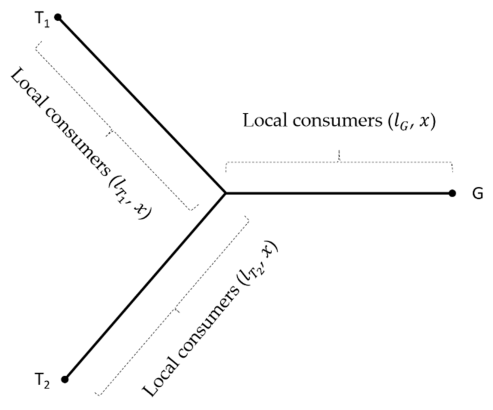
Figure 2.
Marginal consumer (MC) locations in equilibrium.
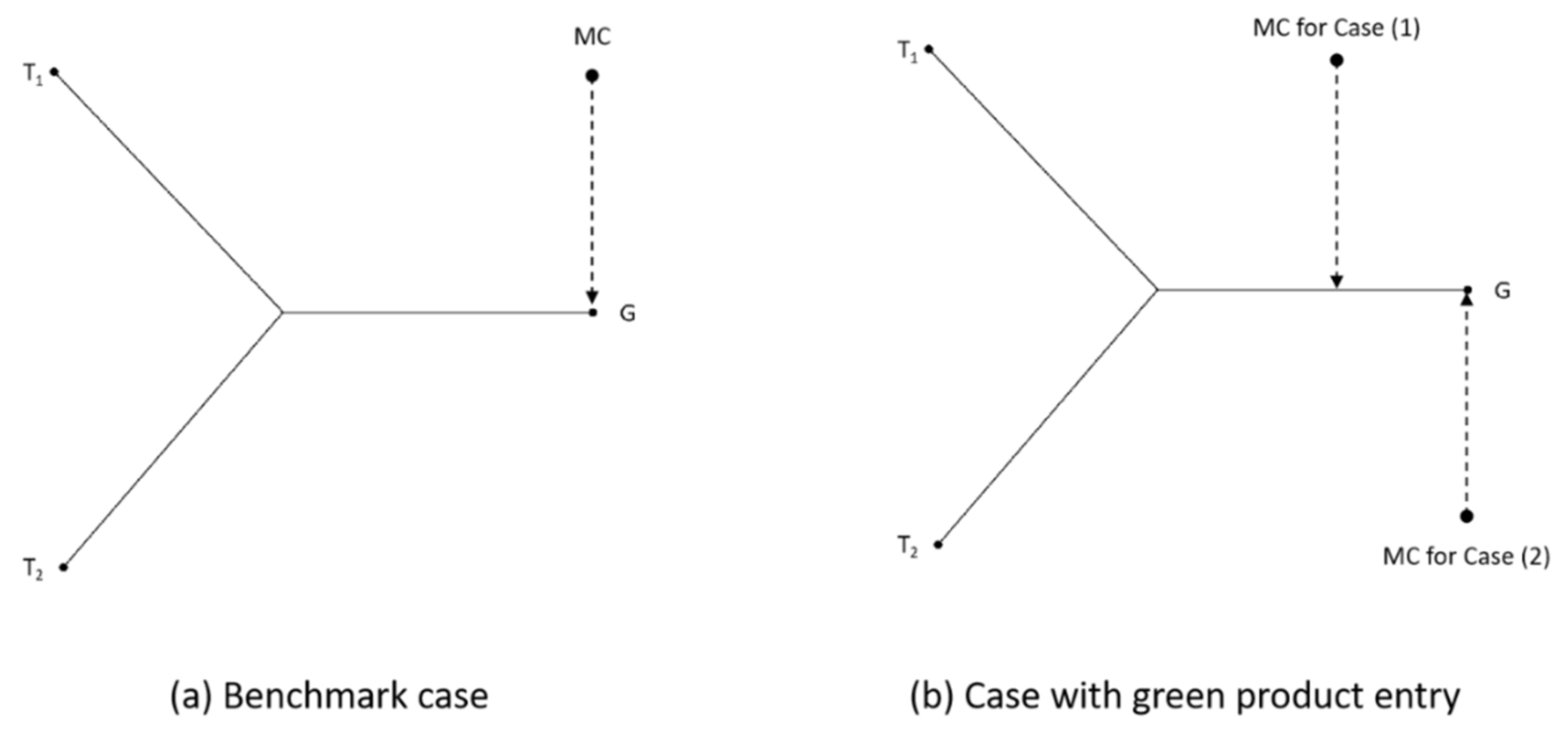
Figure 3.
The impacts of platform fee on the parameter regions.
Publisher’s Note: MDPI stays neutral with regard to jurisdictional claims in published maps and institutional affiliations. |
© 2021 by the authors. Licensee MDPI, Basel, Switzerland. This article is an open access article distributed under the terms and conditions of the Creative Commons Attribution (CC BY) license (https://creativecommons.org/licenses/by/4.0/).
Share and Cite
MDPI and ACS Style
Wang, J.; Gao, X.; Wang, Z. Sustainable Supply Chain Decisions under E-Commerce Platform Marketplace with Competition. Sustainability 2021, 13, 4162. https://doi.org/10.3390/su13084162
AMA Style
Wang J, Gao X, Wang Z. Sustainable Supply Chain Decisions under E-Commerce Platform Marketplace with Competition. Sustainability. 2021; 13(8):4162. https://doi.org/10.3390/su13084162
Chicago/Turabian StyleWang, Junbin, Xuan Gao, and Zhiguo Wang. 2021. "Sustainable Supply Chain Decisions under E-Commerce Platform Marketplace with Competition" Sustainability 13, no. 8: 4162. https://doi.org/10.3390/su13084162
Note that from the first issue of 2016, this journal uses article numbers instead of page numbers. See further details here.