Article

Pre-Positioning Facility Location and Resource Allocation in Humanitarian Relief Operations Considering Deprivation Costs

School of Civil Engineering and Architecture, University of Jinan, Jinan 250022, China
*
Author to whom correspondence should be addressed.
Sustainability 2021, 13(8), 4141; https://doi.org/10.3390/su13084141
Submission received: 1 March 2021 / Revised: 1 April 2021 / Accepted: 2 April 2021 / Published: 8 April 2021

Abstract

:
Alleviating human sufferings during and in the aftermath of disasters is one of the most important goals in humanitarian relief logistics. The lack of relief commodities, especially life-saving items, is a life-threatening loss to victims and must be considered when making emergency supply allocation and transportation decisions, even in the pre-disaster prepositioning phase. This paper proposes a scenario-based stochastic program that integrates the decisions of prepositioning facility locations, quantities of stocked emergency supplies, and service allocations in each scenario in the same modeling framework. The estimation of victims’ losses for waiting for emergency supplies is measured in the typical deprivation cost function and treated as one of the main bases of decision making, besides traditional transportation costs, in determining the service allocation strategies in each scenario. Specifically, a case study with data from the hurricane threat in the Gulf Coast area of the US was conducted to demonstrate the application of this model and the significance of considering victims’ welfare loss in humanitarian relief logistics. Some interesting managerial insights were also drawn from a series of numerical experiments and sensitivity analyses.

1. Introduction

Catastrophic disasters usually bring tremendous damages to the functioning of a community or society, resulting in widespread human, infrastructure, economic or environmental damages beyond the handling ability and resource capacity of the affected area [1]. For example, the 2010 Yushu earthquake in China hit more than 20,000 square kilometers, and infrastructure systems, such as education, health, electricity, communication, highway, and water conservancy, were severely damaged. The total number of people affected by the earthquake reached approximately 200,000, and the number of casualties was about 13,968 [2]. In 2020, a worldwide pandemic of the coronavirus (COVID-19) emerged that caused a large number of casualties and economic losses all over the world, and in the next period, the world will continue to face difficulties. This is the result of a combination of factors, such as fast population growth, overconcentrated populations and infrastructure construction, excessive exploitation of resources, degradation of the natural environment, that jointly lead to vulnerable living areas [3].
When an emergent event happens, the intractable disaster relief work can be better coped with from a humanitarian understanding by providing logistical support for disaster victims, and its main goal is to save lives, alleviate victims’ sufferings, and preserve human dignity. Humanitarian relief logistics can be roughly divided into three stages, pre-disaster preparation, the immediate response at the initial stage of a disaster, and the medium- or long-term humanitarian relief, in the post-disaster phase [4]. The first stage is to take precautions before the attack of a catastrophe, such as making evacuation plans, carrying out emergency training, purchasing rescue necessities, e.g., water, medicine, and tents in temporary resettlement areas. When a disaster happens, a quick response is highly needed and should be carried out immediately, and the focus could be coordinating supplies, estimating damages and humanitarian relief demand, and providing limited humanitarian aid. When more disaster information comes in, targeted emergency rescue activities could be carried out step-by-step in the post-disaster period, mainly including the procurement, transportation, and distribution of the critical supplies needed by the victims and the response activities [5].
In the past decades, extensive research has been carried out on humanitarian logistics. It involves a series of key decisions across these three stages; however, these decisions may affect each other, such as the interaction between the pre-disaster emergency service facility location design and the post-disaster transportation and allocation. Therefore, more research focusing on integrated models is needed to capture the impact of the decisions of a certain stage on the emergency activities of other stages. On the other hand, the decision-making process involves balancing the interests of various parties, especially the interests of the victims, which is the biggest difference between humanitarian logistics and commercial operations [6,7]. The incorporation of victims’ benefits could lead to multiple objectives in the modeling structure and add more challenges. Besides, the lack of accurate information (e.g., actual demand of victim groups, and link availability of disaster areas) brings further challenges and complexity to the problem. These concerns jointly call for more efforts in the study of humanitarian logistics.
In this paper, the integration of facility location and material prepositioning in the pre-disaster planning phase (i.e., strategic level) and service allocation in the post-disaster period (i.e., operational level) was realized in a scenario-based stochastic program (see Figure 1). At the strategic level, the model determines the optimal prepositioning locations and the amount of the preset materials in each facility; while in each scenario, the service allocation will be realized based on the considerations of both transportation cost and deprivation cost. To better characterize the interests of victims during emergency logistics operations, the typical deprivation cost function, proposed by Holguín-Veras et al. was adopted in this paper, and two similar function forms were used to provide a comparative study. To deal with the nonlinear structure of the deprivation cost, a periodical service mode was introduced that enabled us to develop a mixed-integer program to facilitate the calculation. A series of numerical experiments were conducted with the network in the Gulf Coast area of the US to illustrate the performance of our proposed model. Sensitivity analyses were carried out to derive beneficial managerial insights. Our contributions are summarized as follows:
  • A scenario-based stochastic programming model was built. The modeling framework considers the possibility of frequent disaster scenarios and involves a variety of decisions at both strategic (e.g., facility location, material prepositioning) and operational levels across all possible disaster scenarios (e.g., service allocation).
  • The interrelationship between the economic (e.g., facility setup cost, material inventory cost, transportation cost) and social (e.g., victims’ deprivation cost) considerations was explored in the same optimization modeling structure. Three types of typical deprivation cost functions were applied to describe the loss accumulation patterns of the victims and examine the sensitivity of different deprivation cost measurements.
  • Management insights: The numerical results show the significance of the deprivation cost is nonnegligible when making optimal decisions. To reduce the loss of the victims in the humanitarian supply system, emergency storage centers tend to be built locally, and most of the service allocation relationships present simple one-to-one or one-to-two modes to centralize the material supply. Different forms of the deprivation cost function do not have a significant impact on the final optimal solutions, but if the periodical transportation pattern is changed, the optimal solutions will change dramatically. The sensitivity analysis results indicate that when the link travel time of the disaster area increases or the decision-maker puts more focus on the victims’ benefits, more locations and more contracted service modes can be observed. These results might be helpful to better understand the occurrence and progress of humanitarian logistics activities and provide useful references for emergency managers to make decisions.
The remainder of this paper is organized as follows. Section 2 gives a literature review on this topic. Section 3 presents the notation and formulation of the scenario-based stochastic program and puts forward cost components to build the model structure. Additionally, more considerations on the deprivation cost are introduced as model extensions. Section 4 discusses the results from a sequence of numerical experiments. Section 5 draws some conclusions and briefly goes into future research directions.

2. Literature Review

Since the main research scope includes the emergency service facility location, relief material prepositioning, service allocation, and the considerations of the personal interests of victims in humanitarian logistics, the literature is reviewed in these aspects.
The efficiency of humanistic logistics operations is affected by many factors, which is a system optimization problem. Due to the complexity and uncertainty of the disaster environment, it usually brings great challenges to the decision-making process. For instance, the number of materials needed by victims is usually not able to be accurately predicted, and as a result, material shortage or oversupply often occurs. If the humanitarian relief measures are not in place in a timely manner or the emergency supplies are seriously lacking, the phenomenon of the scramble for supplies might occur due to the panic. The infrastructure system may be severely damaged in the disaster area, causing communication disruption, road destruction, and lack of water and electricity, etc. Holguín-Veras and Jaller [8] made a numerical estimation of resource demand and its temporal pattern based on a set of data from the emergency responders of Hurricane Katrina and estimated the resource requirements through the robust autoregressive integrative moving average models. Rawls and Turnquist [9] proposed a two-stage stochastic mixed-integer programming model that considered the uncertainty of emergency demand, the proportion of available materials in the prepositioning facilities, and the availability of a transportation network after an event. In the context of disasters, the limited and unpredictable information also greatly increases the difficulty of disaster response. Besiou et al. [10] believed that humanitarian logistics operations were affected by many factors, such as time pressure, resource scarcity, and uncertainty, and that system dynamic modeling (SD) was an effective way to address the complexity of humanitarian logistics. Besides, to cope with these challenges, many system optimization problems have been studied to capture the characteristics of disaster environments and to try to reach an optimal or approximate optimal arrangement for emergency logistics operations. Khayal et al. [11] put forward an optimization model for temporary facility location and resource allocation based on the consideration of the change of emergency relief demand and supply over time. Moreno et al. [12] proposed a two-stage scenario-based approach for relief distribution that combines the key decisions, such as relief center locations, emergency commodity distributions, and fleet sizing, in two stages. The uncertainty raised in commodity supply, proportion of available materials, demand, and routes were taken into account in the study. Khorram-Manesh et al. [13] pointed out that to ensure that the victims can receive continuous medical assistance, alternative leadership, and rescue facilities can be set-up in the community in the future to take care of the minorly wounded to reduce the burden on the hospital.
The primary purpose of emergency response activities is to mitigate the loss of life and property in the affected areas as much as possible. Therefore, when making these key decisions, the interests of the victims also need to be considered, in other words, the maximum operating efficiency and minimum human sufferings should be considered at the same level, including how to measure the loss of the victims when undertaking disaster risks and how to integrate these social benefits into the decision-making process. The concept of deprivation cost was first put forward by Holguín-Veras et al. [14] to characterize the interest of victims as the economic value of the human sufferings caused by a lack of access to goods or services. Holguín-Veras et al. assumed that the deprivation cost functions were expected to be (1) monotonic, nonlinear, and convex to the deprivation time; (2) associated with non-additive demands and, possibly, hysteretic effects that reflect residual damage to the beneficiaries. A contingent valuation experiment was further used to estimate the form of the deprivation cost function by Holguín-Veras et al. [15]. Their approach was based on how much a person was willing to pay for critical supplies or services to reduce the probability of death. The results proved that the deprivation cost (e.g., drinkable water) increased nonlinearly with deprivation time. Cantillo et al. used discrete choice theory to evaluate the deprivation cost generated by the delivery of basic goods after disasters, and it was proved that the externalities (i.e., deprivation cost) caused by delayed delivery of basic goods showed a nonlinear structure, strictly increasing, and convexity in the deprivation time. Adding socioeconomic variables, such as age and gender, to the model revealed differences in the values of deprivation time and explained differences in individual preferences [16]. Cotes and Cantillo utilized the consumer surplus equation to calculate the deprivation cost function [17]. Zhu et al. considered relative and absolute deprivation costs, and the deprivation cost function was determined by the exponential growth function obtained by Holguín-Veras et al. [18]. Shao et al. analyzed the current situation of the deprivation cost and discussed the key issues in the study of the deprivation cost from the aspects of estimation methods, the application of the deprivation cost, estimation differences, challenges, and obstacles [19].
Usually, the deprivation costs are integrated into the optimization model of humanitarian logistics. For example, operational costs and deprivation costs are incorporated into the decision-making process. The formulas for the allocation of limited commodities were proposed to reduce the total social costs and human sufferings [5]. A facility location model for pre-disaster supplies was developed by Cotes and Cantillo to determine the number of items to be prepositioned to serve the affected area, and the key feature of the model formulation is about the considerations of the deprivation cost [17]. To obtain the optimal emergency relief routing strategy, Zhu et al. [18] established two models with different injured degrees and considered the equity and priority issues through the deprivation cost. The benefits of the victims are also measured in other forms. For instance, on the premise of considering the risk of service interruption, An et al. [20] made a reliable evacuation pickup facility location and service allocation strategy for transit-based evacuation and the exposure risks of the evacuees in the pickup facility were measured and taken as a cost component in the model objective. Yu et al. [21] proposed another three measures related to the benefits of the victims (i.e., efficiency, effectiveness, and equity) in the humanitarian aid, and the deprived state was valued from the last acquisition to the current period. From another angle of humanization, Macpherson et al. [22] proposed that humanitarian relief workers, as the first responders after disaster events, should be paid more attention to their mental health problems and establish an organizational framework for their mental health and psychosocial support.

3. Problem Description and Model Formulation

In this section, a scenario-based stochastic program for humanitarian logistics service problems is given, which simultaneously addresses emergency storage facility location and material prepositioning decisions in the pre-disaster period and service allocation in the post-disaster phase across all possible disaster scenarios.

3.1. Notations and Problem Description

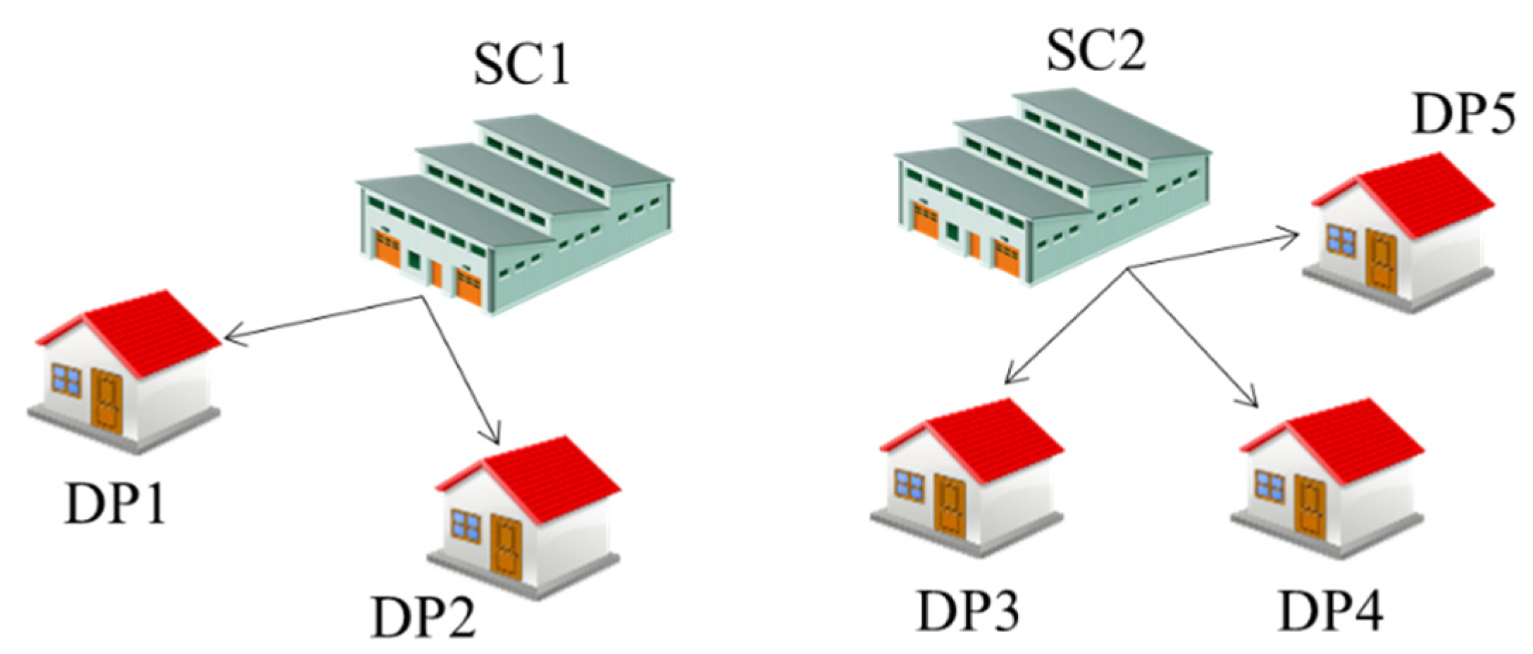
In the aftermath of a disaster, it is assumed that there are a set of victim groups, J, spreading over the disaster-affected area, and their locations could be temporary resettlements, shelters, medical centers, or just stopovers. For each victim group j J , the estimated number of victims is denoted as P j . To mitigate the life and property losses of victims, it is necessary to provide emergency materials for them. Given that a series of candidate storage centers located around or within the disaster area (low-risk areas) can be potentially selected to carry out the emergency logistics tasks and the whole set can be indexed by I . The transportation pattern between each pair of supply and demand nodes is assumed to follow the one-to-many periodical service mode. In other words, each victim group can be served by only one single supply point, but each storage center can provide service for several demand points, and the service is going continuously in a circular way (see Figure 2).
For each candidate storage center i I , its storage capacity is M i , and if it is selected as a supplier of the emergency logistics service network, it needs a fixed set-up cost F i to sustain operations. The facility location decisions are represented by a set of binary variables y = { y i | i I } , where
y i = { 1 if   facilty   i   is   selected   as   a   storage   center 0 otherwise ,
then the total facility setup cost is i I F i y i .
As a part of the emergency activities in the emergency preparatory phase, prepositioning a certain amount of common-use emergency materials at each selected storage center is one efficient way to provide rapid support for the neighboring disaster-affected areas in the initial emergency response phase. The set of commodities that would be prepositioned at each storage center are denoted by K, indexed by k K . Let η k be the unit storage space required for commodity k and q i k be the unit commodity handling cost for commodity k at location i, which may include procurement costs of commodities, transportation costs from product suppliers to storage centers, and the maintenance cost for one unit of the commodity in the pre-disaster phase. Assuming that the consumption rate ρ k of commodity k in the disaster-affected area (e.g., every 24 h) is known, it is assumed the same for all victims, regardless of age, sex, etc. The key prepositioning decisions (i.e., the total amount of commodities prepositioned in the storage center) are denoted by variables r = { r i k | i I , k K } , then the total commodity prepositioning cost is k K i I q i k r i k .
For each disaster-prone area, various disaster situations could happen, and these discrete scenarios can be denoted by set S, indexed by s S . The probability of each scenario s is represented as p s , and the probability could be related to different commodity demands, link availability, and road network conditions, etc. The total commodity demand d j k s of victim group j for commodity k in scenario s is estimated by the group population and the average commodity consumption rate. In each scenario, commodities are delivered directly from storage centers to victim groups, and the delivery mode is assumed to be the one-to-many service, i.e., one storage center can provide service for multiple groups. The service allocation decisions are expressed by binary variables x = { x i j k s | i I , j J , k K , s S } , where
x i j k s = { 1 if   facility   i   provides   commodity   k   for     demand   point   j   in   scenario   s 0 otherwise .
The travel distance D i j between each storage center i to victim group j can be linked together through any of the actual distances between two points, which can be further calculated to travel time t i j . The unit transportation cost for delivering one unit of commodity k from storage center i to victim group j in scenario s is denoted as c i j k s . Based on the total commodity demand estimation, the total transportation cost between storage center i to victim group j in each scenario s is i I j J k K x i j k s c i j k s D i j d j k s .
Let Q i j s be the available capacity of the link (i, j) in scenario s, which completely depends on the link connectivity and serviceable conditions under the attack of disasters, and a coefficient μ k is used to convert the transportation amount into traffic flow for commodity k passing through each link.

3.2. Deprivation Costs in Humanitarian Relief

The main purpose of humanitarian logistics is to provide the necessary disaster relief supplies and timely humanitarian aid for victims’ right after the attack of disasters to alleviate victims’ sufferings and reduce their life and property losses. During this process, the logistics network design and operation patterns would directly affect the subjective feelings and individual benefits of victims. The economic efficiency would not be the exclusive concern for both logistics managers and government but also the social benefits and costs of the affected groups. This is a major difference between humanitarian and commercial logistics. Thus, it makes sense to integrate the victims’ sufferings caused by the lack of relief supplies into the decision-making process and express it in terms of social cost (e.g., deprivation cost) to make a trade-off between economic and social considerations.
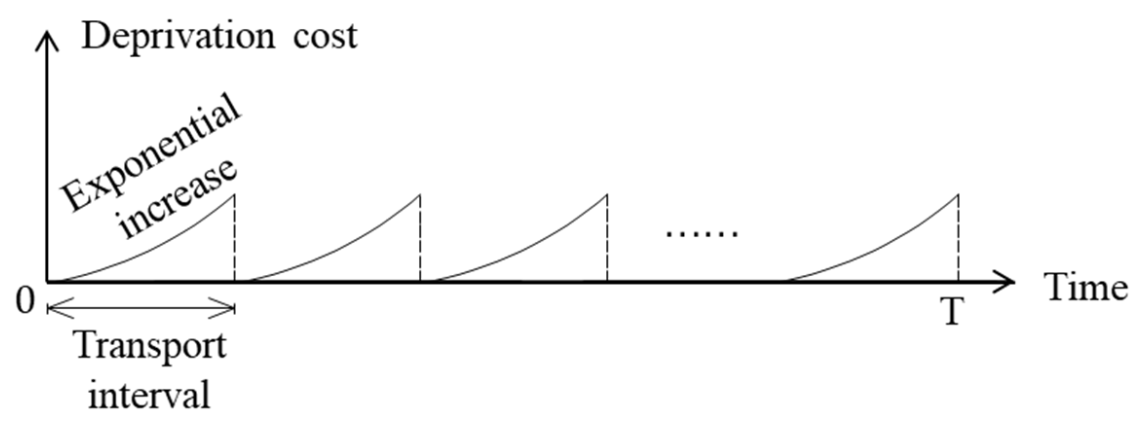
After a disaster occurs, periodical and continual supplies for each affected group are needed. During each roundtrip, there is always a waiting period for victims waiting for the subsequent humanitarian aid. It is a kind of “deprivation” of supplies for victims. Figure 3 shows the curve of the deprivation cost at a certain demand point over time with the periodical supply of some emergency commodity, where the exponential growth part is derived from the empirical function [20]. To simplify the problem analysis, it is reasonable to assume that the deprivation cost of each affected group starts to accumulate from time zero (i.e., zero point at horizontal time axis). At this moment, the emergency vehicles also start from storage centers, so the maximum waiting time of affected group j is equal to the transportation time between storage center i and this demand point.
Holguín-Veras et al. [20] defined the hysteretic case of the deprivation cost, i.e., the deprivation effect does not disappear promptly after the demand is fulfilled. In other words, when the humanitarian relief supplies arrive at a demand point, the deprivation cost of the victims at this demand point does not drop to zero directly but will decrease with a constant rate of commodity consumption. To simplify this description, the decline phase of the deprivation cost is characterized as a linear process, as the linear pattern shown in Figure 3. It is related to the commodity consumption time. Thus, the calculation of deprivation cost in one wavy circle can be determined by the sum of the exponential increase accumulated over the vehicle travel time and the linear decrease across the commodity consumption period.
Humanitarian relief should be rolling on in circles during the emergency rescue period T , e.g., the first three days (72 h) after the attack of a disaster [23]. For each demand point/affected group, if all the periodical deliveries of a certain commodity repeat the same pattern within the given emergency rescue period, T , a series of identical curves (i.e., growing exponentially at the same rate as the previous circle and going down linearly) can be obtained until it reaches the end of the emergency rescue period T .
Let θ i j k s be the delivery frequency of commodity k from storage center i to demand point j in scenario s. Then for the demand point j, the amount of one-time delivery is expressed as d j k s θ i j k s . Since the total material consumption rate of demand point j in each service cycle is ρ k P j 24 , the material consumption time is calculated as 24 d j k s θ i j k s ρ k P j . As shown in Figure 3, for the duration of one service cycle, the following equation can be obtained, i.e., t i j + 24 d j k s θ i j k s ρ k P j = T θ i j k s , and the delivery frequency θ i j k s can be derived below.
θ i j k s = T ρ k P j 24 d j k s ρ k P j t i j , i I , j J , k K , s S
By following the deprivation cost function of Holguín-Veras et al. [20], the probability density function of the deprivation cost is shown below to describe the exponential growth part in Figure 3, where a j k s and b j k s are the coefficients of the deprivation cost accumulation curve of victim group j for commodity k in scenario s.
f ( t ) = e a j k s t + b j k s e b j k s , ( 0 t t i j )
Within each service interval, the total deprivation cost suffered by the disaster victims equals the deprivation cost accumulated in the process of both material transportation and consumption, i.e., considering the hysteretic effect of deprivation suffered by the disaster victims. Thus, the total deprivation cost Γ i j k s of affected group j in each service interval for “depriving” commodity k in scenario s can be obtained by the integral sum of two parts as follows.
Γ i j k s = P j ( 0 t i j f ( t ) d t + S Δ A B C ) = P j 0 t i j ( e a j k s t + b j k s e b j k s ) d t + ( e a j k s t i j + b j k s e b j k s ) 12 d j k s θ i j k s ρ k , i I , j J , k K , s S
Then, the total deprivation cost in one service circle across all the affected groups is
i , j , k x i j k s Γ i j k s = i I j J k K x i j k s ( P j e b j k s ( e a j k s t i j 1 a j k s t i j a j k s ) + ( e a j k s t i j + b j k s e b j k s ) 12 d j k s θ i j k s ρ k ) , i I , j J , k K , s S
When summarizing all the cost components based on the parameters and decision variables described above, the total expected system cost across all the potential scenarios can be formulated as follows.
When summarizing all the cost components based on the parameters and decision variables described above, the total expected system cost across all the potential scenarios can be formulated as the sum of the facility location cost i I F i y i , material prepositioning cost k K i I q i k r i k , material allocation and transportation cost s S i I j J k K p s x i j k s c i j k s D i j d j k s , and the victims’ deprivation cost s S i I j J k K p s β x i j k s Γ i j k s θ i j k s as follows.
Φ ( x , y , r ) : = i I F i y i + k K i I q i k r i k + s S p s ( i I j J k K x i j k s c i j k s D i j d j k s + i I j J k K β x i j k s Γ i j k s θ i j k s )
The scenario-based emergency prepositioning facility location and service allocation model is to minimize the total system costs across all scenarios, including facility set-up cost, material prepositioning cost, transportation cost, and victims’ deprivation cost. Through optimal design, it determines the optimal prepositioning facility locations { y i } , material prepositioning decisions { r i k } , and supply-to-demand service allocations in each scenario { x i j k s } .
The model can be formulated as follows:
Min x , y , r i I F i y i + k K i I q i k r i k + s S p s ( i I j J k K x i j k s c i j k s D i j d j k s + i I j J k K β x i j k s Γ i j k s θ i j k s )
Subject to:
k K η k r i k M i y i , i I
i N x i j k s = 1 , j J , k K , s S
j N x i j k s d j k s r i k , i I , k K , s S
x i j k s y i , i I , j J , k K , s S
j N d j k s i N r i k , k K , s S
k K x i j k s μ k d j k s ρ k P j t i j T ρ k P j 24 d j k s Q i j s , i I , j J , s S
y i ( 0 , 1 ) , i I
x i j k s ( 0 , 1 ) , i I , j J , k K , s S
r i k 0 , i I , k K
The objective Function (6) aims to minimize the total expected system cost incurred in both the pre-disaster and post-disaster phases. The coefficient β is used to represent the weight of deprivation cost in the total system cost. Constraints (7) ensure that if the prepositioning facility/storage center i is selected, the space occupied by preset commodities will not exceed its facility capacity. Constraints (8) enforce that in scenario s, each victim group j J will be assigned to one storage center to obtain a certain kind of commodity. Constraints (9) guarantee that the total demands within the service range of each storage center do not exceed its total prepositioned quantity. Constraints (10) refer to a storage center that should be set-up before assigned to a victim group. Constraints (11) show the demand conservation in the logistics operation system. Constraints (12) reveal that the link flow cannot exceed its capacity, even if the link capacity may be discounted due to the disaster. Constraints (13)–(15) spell out all binary and nonnegative variables.

3.3. More Considerations on the Deprivation Cost

In the above section, a specific form of the deprivation cost function was adopted to describe the losses of the victims, i.e., the exponential increase before the arrival of the emergency supplies and the linear decrease in the supply consumption phase. However, various forms of the losses of the victims might occur in practice with the execution of different emergency delivery strategies, and there could be several deprivation cost functions that may be used to describe these loss accumulation patterns. In this section, a few more forms of deprivation cost functions are discussed to examine the sensitivity of different deprivation cost measurements.
(1)
Exponential growth only and no hysteretic effect
Despite the wide acceptance and adoption of the exponential form of the deprivation cost in the loss accumulation phase in previous studies, the declining stage of the deprivation cost could be considered in different ways. For instance, the curve of deprivation cost over time is shown in Figure 4. The deprivation cost function is thought to be in the form of exponential growth, but the hysteresis of the “deprivation” is not taken into consideration. In other words, once the relief items reach demand points, the sufferings of the victims are assumed to disappear immediately, i.e., there is no hysteretic effect [21]. Following this pattern, the duration taken in each loss increase phase could include vehicle travel time, supply loading time, and delivery breaks, etc. This parameter can be marked as t i j * . Thus, the delivery frequency θ i j k s is obtained below.
θ i j k s = T t i j * , i I , j J , k K , s S .
If the number of transport vehicles is sufficient, there may be a scenario where once the transport vehicle in the previous cycle arrives at the demand point, the vehicle in the next cycle heading to the same demand point will set off at the same time. Under these circumstances, the duration t i j * is equal to the travel time t i j from node i to j.
The deprivation cost in each cycle can be calculated by taking the same probability density function of the exponential function that was used before, where
f ( t ) = e a j k s t + b j k s e b j k s , ( 0 t t i j * ) .
The total deprivation cost Γ i j k s of affected group j in each service interval for “depriving” commodity k in scenario s is calculated by integral of only one exponential growth part as follows:
Γ i j k s = P j 0 t i j * ( e a j k s t + b j k s e b j k s ) d t , i I , j J , k K , s S .
That is,
Γ i j k s = P j e b j k s ( e a j k s t i j 1 a j k s t i j * a j k s ) , i I , j J , k K , s S .
Update the delivery frequency θ i j k s from T ρ k P j 24 d j k s ρ k P j t i j to T t i j * to reflect the non-hysteresis effect, and the capacity constraints (12) changed to:
k K x i j k s μ k d j k s t i j * T Q i j s , i I , j J , s S
When substituting the deprivation cost component into Model (6), Model (21) is presented below.
Min x , y , r i I F i y i + k K i I q i k r i k + s S p s ( i I j J k K x i j k s c i j k s D i j d j k s + i I j J k K β x i j k s P j e b j k s ( e a j k s t i j 1 a j k s t i j * a j k s ) θ i j k s )
subject to: (7)–(11), (13)–(15), and (20).
(2)
Quadratic growth with hysteretic effect
The form of exponential growth is a good way to describe the increase and accumulation of victims’ losses over time, but if incorporating this form in the modeling framework, often brings challenges to the solution techniques. Therefore, it leads us to the idea of finding other ways to replace this nonlinear part or to test the difference between this typical formulation and other function forms.
An alternative expression is using a quadratic function to approximate the deprivation cost, and the hysteretic effect of the victims consuming relief items is also considered after the arrival of relief items, as shown in Figure 5. In other words, the deprivation cost in each transport cycle accumulates as a quadratic increasing form and then declines linearly. Due to the considerations of the hysteretic effect, there is no change in the formulation of the delivery frequency θ i j k s compared to Equation (1). The slope of the linear decline phase is equal to the consumption rate of the victims and the material consumption time is 24 d j k s θ i j k s ρ k P j .
The probability density function of the quadratic growth is shown below, where h j k s is the coefficient of the deprivation cost accumulation curve of victim group j for commodity k in scenario s.
f ( t ) = h j k s t 2 , ( 0 t t i j ) .
Similarly, the total deprivation cost Γ i j k s of affected group j in each service interval for “depriving” commodity k in scenario s can be obtained by the integral sum of two parts as follows:
Γ i j k s = P j ( 0 t i j f ( t ) d t + S Δ A B C ) = 1 3 P j h j k s t i j 3 + 12 d j k s θ i j k s ρ k h j k s t i j 2 , i I , j J , k K , s S
With the substitution of the deprivation cost component in Model (6), Model (24) is shown below.
Min x , y , r i I F i y i + k K i I q i k r i k + s S p s ( i I j J k K x i j k s c i j k s D i j d j k s + i I j J k K β x i j k s ( 1 3 P j h j k s t i j 3 + 12 d j k s θ i j k s ρ k h j k s t i j 2 ) θ i j k s )
subject to: (7)–(15).

4. Numerical Study

In this section, an experimental road network in the Gulf Coast area of the US with a hurricane threat was applied to conduct numerical experiments, including 30 nodes and 58 links (Rawls and Turnquist [9]). The historical records of 15 hurricane events and 51 scenarios (including both separate events and joint events) generated in Rawls and Turnquist’s study continues to be used in this paper as well as the probability of occurrence of each scenario. The setting of the disaster scenarios provides information about disaster attack sites, their emergency material demands, and the occurrence probability of each scenario. With these basic inputs, a set of cases with different emergency demands are set to test the effect of demand uncertainty on the optimal solutions. Besides, three forms of deprivation cost functions are considered separately in the modeling structure to verify the significance of incorporating the interest of victims in the decision-making process. A series of sensitivity analyses concerning several key parameters of the proposed mixed-integer program (MIP) model is shown to examine their impacts and draw insights. All models and cases are coded in GAMS 25.1.3 and run via the solver CPLEX on a PC with 2.79 GHZ CPU and 4.00 GB RAM.

4.1. Basic Parameter Settings

In the case study, three kinds of emergency relief supplies: water, food, and medical kits were considered, and their units were 1000 gallons, 1000 meals, and 1000 kits. The unit commodity handling cost q i k for commodity k at location i follow a random distribution of [$100, $130], [$250, $300], and [$11,400, $14,500], respectively. Correspondingly, the other same parameter settings are summarized in Table 1, e.g., the storage space η k , consumption rate ρ k , transportation cost c i j k s , and coefficient μ k for one unit of emergency relief supplies. The values of consumption rate ρ k and coefficient μ k were given based on the following assumptions: (1) a victim consumes four bottles of water, three meals, and one medical kit every day; (2) each transport vehicle weighs 10 tons with a size of 9.6 m × 2.3 m × 2.4 m.
The fixed set-up cost of each storage center F i and its capacity M i are both hard to give exact values. Assuming that they take values from the following random distribution intervals, i.e., F i follow the random distribution of [$150,000, $200,000], and M i follow [370,000 f t 3 , 420,000 f t 3 ].
The nodes in the experimental network are real cities, so the travel distance of each link can be estimated easily from Google Maps. The distance between any connected two points was determined by the actual distance. Given that in the post-disaster stage, emergency vehicles travel at 50 miles per hour, the travel time between two adjacent nodes, t i j , can be obtained on this basis. Table 2 shows the population of each demand point, P j , after the disaster. No loss of generality, assuming that only a fraction of the population at the demand points were affected.
According to the deprivation cost function of drinking water proposed by Holguín-Veras et al. [20], appropriate coefficient estimates for food and medical kits were made with the common understanding of the importance of food and medicine compared to drinking water, and the data are summarized in Table 3.

4.2. Numerical Experiments When Considering Demand Uncertainty

Mostly the emergency relief demand of each affected area was estimated based on the local population, and, usually, it is very hard to have an exact value due to the complex disaster environment. Even if accurate values on the emergency demand are given, the transportation strategy made based on these needs may be inflexible under actual disaster conditions. To deal with this challenge, a lot of relevant research has been conducted in the past. For instance, to capture the uncertainty of emergency demand, Ni et al. proposed a min–max robust model, and after a series of deduction and verification, they claimed that the demand space was a polyhedron, and its extreme points were at the vertex (Ni et al. [2]). Based on this conclusion, the vertex of the polyhedron can be selected as the extreme points of emergency demand, especially for robust analysis. In this study, considering the following three cases: (1) the worst case (maximum demand); (2) the most likely case (average demand, benchmark case); and (3) the minimum case (minimum demand), to examine the effect of demand uncertainty on the optimal emergency logistics network design and transportation strategy.
To estimate the emergency demand in the three cases as accurately as possible, a database of historical data on various types of disasters was used, including date, location, disaster intensity, and socio-economic data, [24] to get the indispensable statistical data for calculating the emergency relief needs in the post-disaster phase, e.g., the total number of casualties, affected population, and estimates of economic losses. For example, disaster statistics from IFIS [25] showed that in the decade from 1995 to 2004, nearly 6000 disasters were recorded, and they resulted in about 900,000 deaths, $738 billion of material losses and 2.5 billion people affected, accounting for 0.036% of the total population. When typhoon “Haiyan” hit the Philippines, it led to the casualties of more than 36,050 people and the temporary displacement of about 4 million, accounting for about 0.90% of the total population [26]. Between the years 2005 and 2014, according to the world disaster report 2015, flood disasters were the most frequent disasters worldwide, bringing approximately 59,092 deaths, and 866,417 people were affected, accounting for 6.82% of the total population [27,28]. More data on the proportion of people affected in a disaster can be found, e.g., 3.6% in Hurricane “Matthew”, 1.93% in Nepal floods, 6.98% in the Yushu earthquake, etc.
According to the above statistics, the proportion of people affected can be inferred to conduct the numerical experiments, e.g., a proportional value of 2.77% (an average estimate of the above data) is used in this study. On this basis, a range of possible demand values can be deduced in combination with Ni’s theory. For instance, in the worst case, about double the demand is assumed, i.e., double victims or each victim is assigned seven bottles of water, six meals, and three medical kits a day, which represents the highest demand; while in the minimum case, a share of one bottle of water, one meal, and half a medical kit for one victim a day is considered to describe the lowest demand. They are the extreme points of the demand space. According to Ni’s theory, in the most likely case, the amount of relief commodities needed by one victim per day is the average of the maximum and minimum demands. In each scenario, the random distribution within the range of minimum and maximum demands is applied to generate the emergency commodity demand of each demand node.
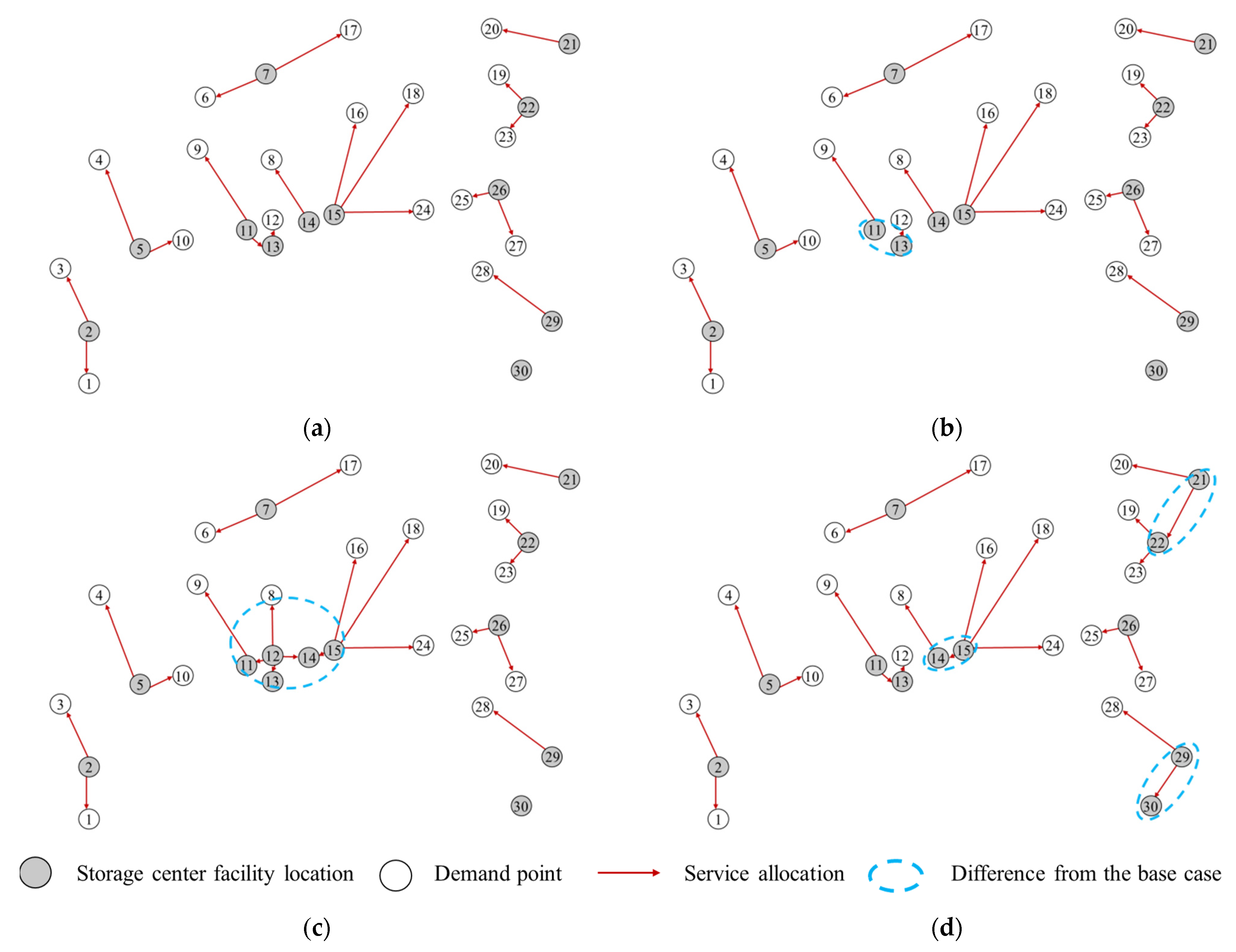
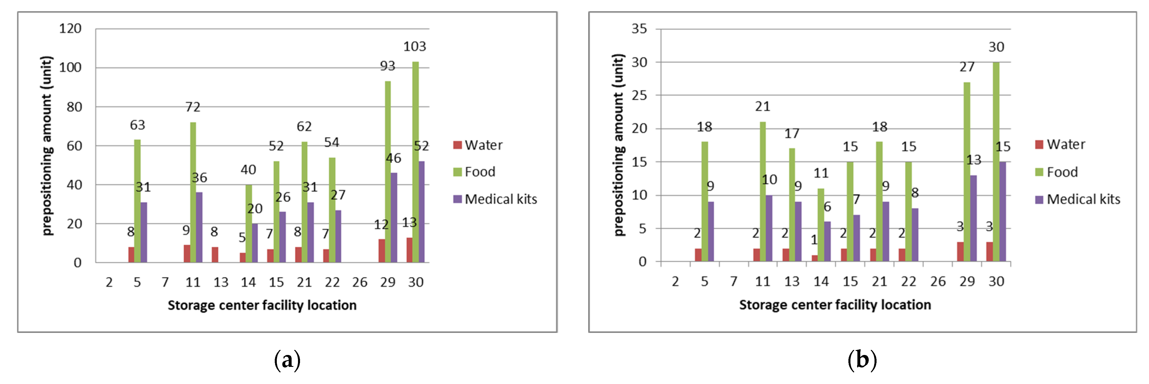
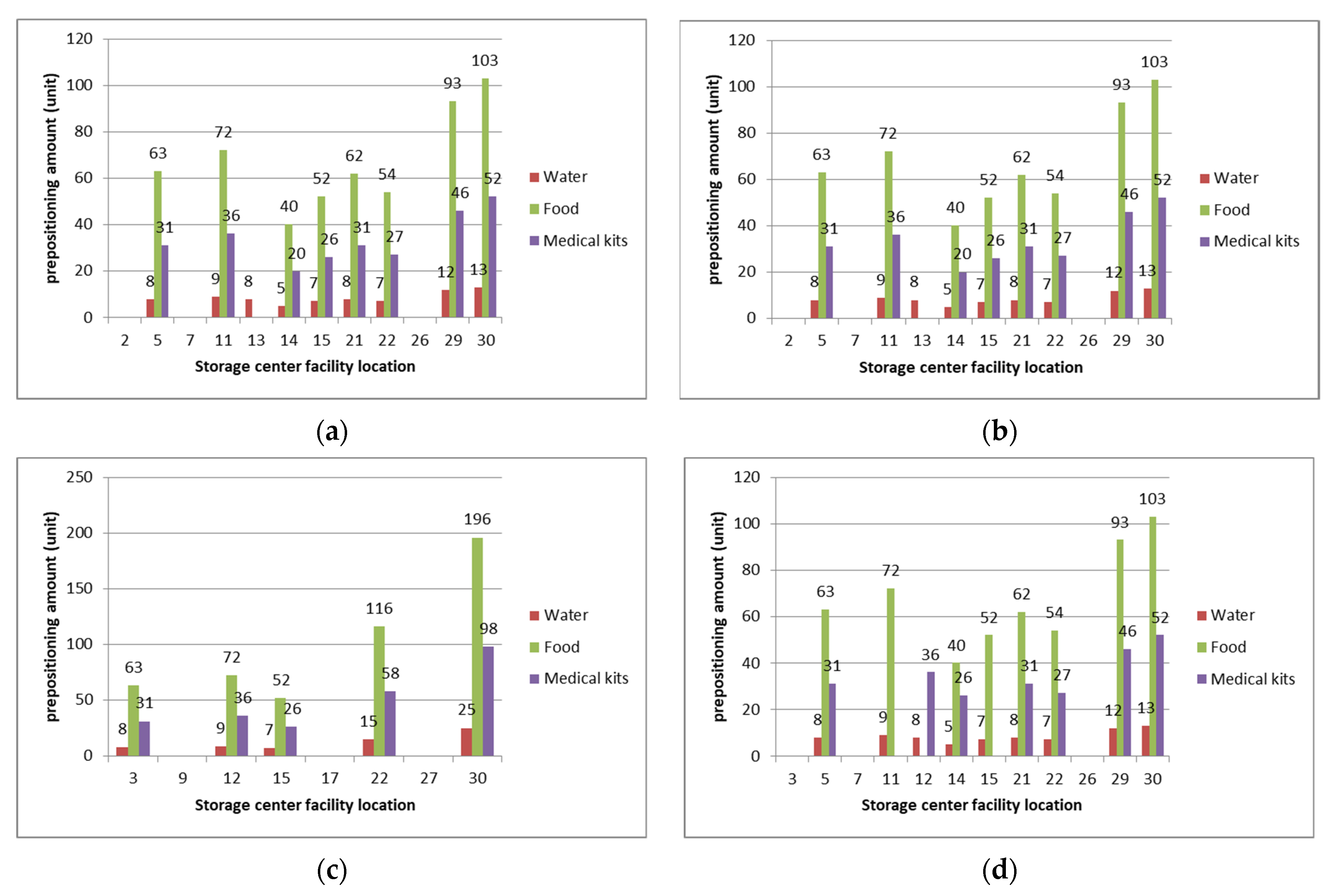
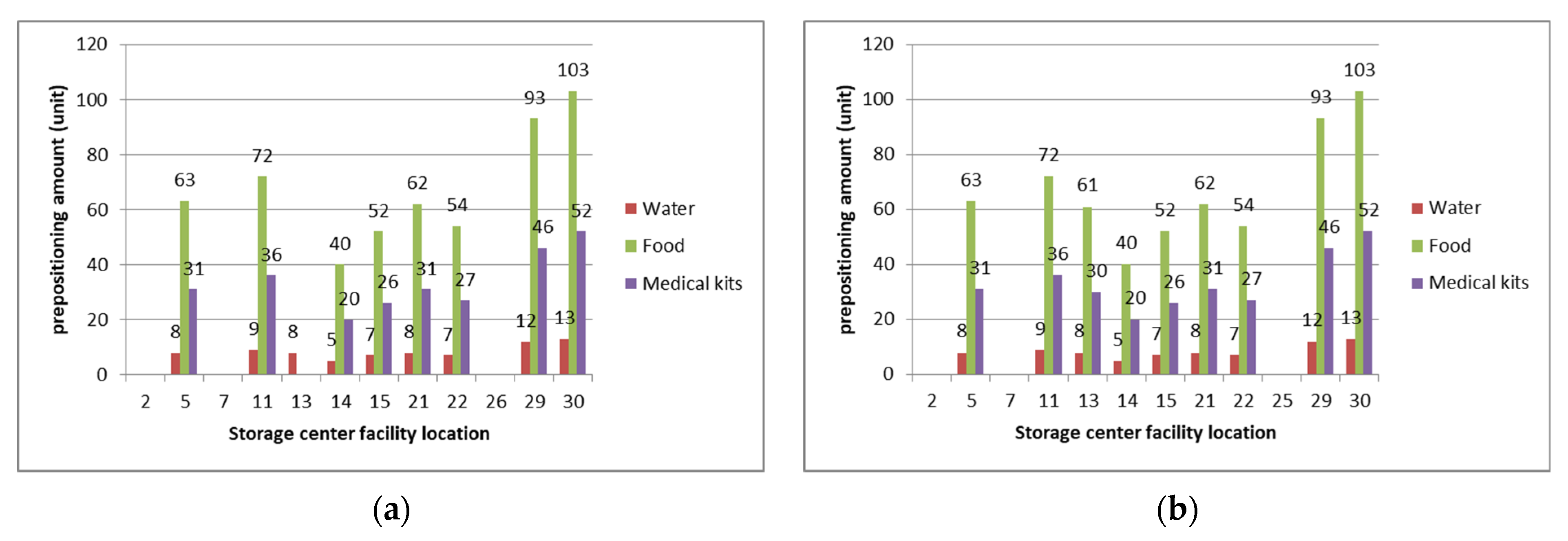
Figure A1 and Figure A2 in Appendix A show the optimization results of the above three cases, including the optimal locations of emergency prepositioning facility locations (grey nodes), prepositioned quantities of various supplies (i.e., small pink, yellow, and green blocks next to the optimal locations to represent water, food, and medical kits, respectively), and service assignments (red arrows). Table A1 further lists the cost components of optimal solutions.
As can be seen from Table A1, the proportion of the transportation cost in the total cost was very small and almost negligible, particularly under emergency situations. It complies with the fact that in the real operations of emergency logistics, transportation costs are usually not the focus of attention. While the costs of material prepositioning (i.e., handling cost) and consideration of victims’ interests (i.e., deprivation cost) account for a large part of the total system cost. It reveals that there is a positive correlation between material prepositioning and total emergency demand. However, experimental results show that the deprivation cost occupies about 22–44% of the total cost, which further confirms the significance of considering the interests of the victims in the modeling system.
Besides, the results also indicate that in all the cases, there is an emergency storage center established in each disaster-prone area. This partly results from the parameter settings (e.g., only a part of the demand points has positive demand inputs), and more important, it is a result of the considerations of the deprivation cost of victims in the modeling framework. In other words, although a disaster-prone area (i.e., a demand point with a positive number of victims) is within the scope of a disaster-affected area and has certain risks, it tends to establish an emergency storage center locally to facilitate the supply of relief materials and reduce the loss of victims to the greatest extent. These storage points provide relief items both for the surrounding disaster areas and themselves to meet the emergency needs in the post-disaster phase. Figure A1 and Figure A2 show that some location and allocation decisions have been involved even in some areas without disaster victims, such as nodes 2, 7, and 26, and there are no emergency supplies prepositioned at these points. This may be because in the current case study, there is no demand set at these supply points and their surrounding demand points, i.e., the emergency service demands of all these points are zero. However, according to the optimization rules, the model also prepares location and allocation results for these points. The optimal service relationship can provide a reference for emergency service in an actual disaster situation.
By comparing the three demand situations, the locations of emergency storage centers only slightly change across the whole region with the settings of different demands. For example, in the minimum demand, average demand, and even the random demand cases, the locations of the optimal emergency storage centers and their total number are completely the same, and only an extra location, node 12, is selected in the maximum demand case. Thus, it can be inferred that although an exact estimate on the emergency demand under disaster conditions is hard to get, as long as accurate historical data on the disaster affected areas and emergency demands are obtained, the locations of emergency storage centers can be determined based on vague estimations in a real case. However, it is apparently that with the change in demand levels, the number of materials prepositioned in each storage center will change. The service allocation relationships also present some changes that are mainly reflected in some storage points with a shortage of preset materials. The insufficient part is usually made up of the nearby storage points, and the difference is shown by the blue dotted line in Figure A1 and Figure A2. For example, in the minimum case, nodes 11 and 13 only need to support the own demands of the these points and one neighbor node at most, but when the emergency demands increases to the average level, a service allocation relationship from node 11 to node 13 is established; while with the continual increase in emergency demand to the maximum level, their resources are unable to meet the needs, an extra node, 12, is selected to provide a centralized supply for neighbor nodes 8, 11, 13, and 14.

4.3. Numerical Results of Different Deprivation Cost Functions

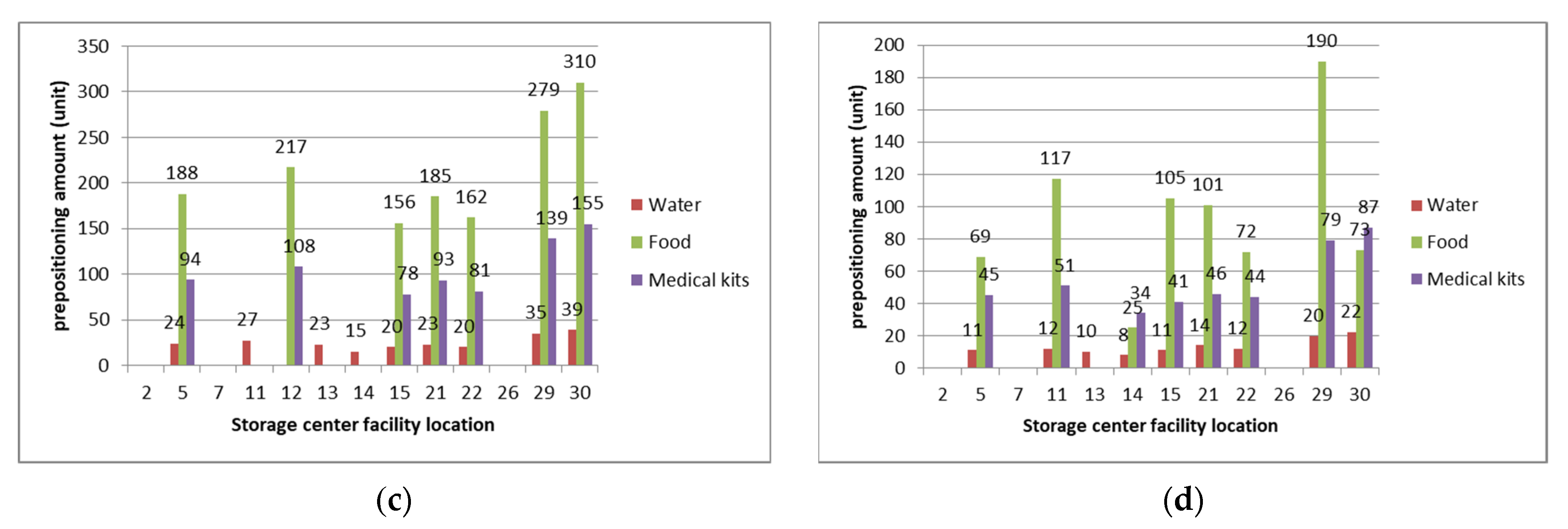
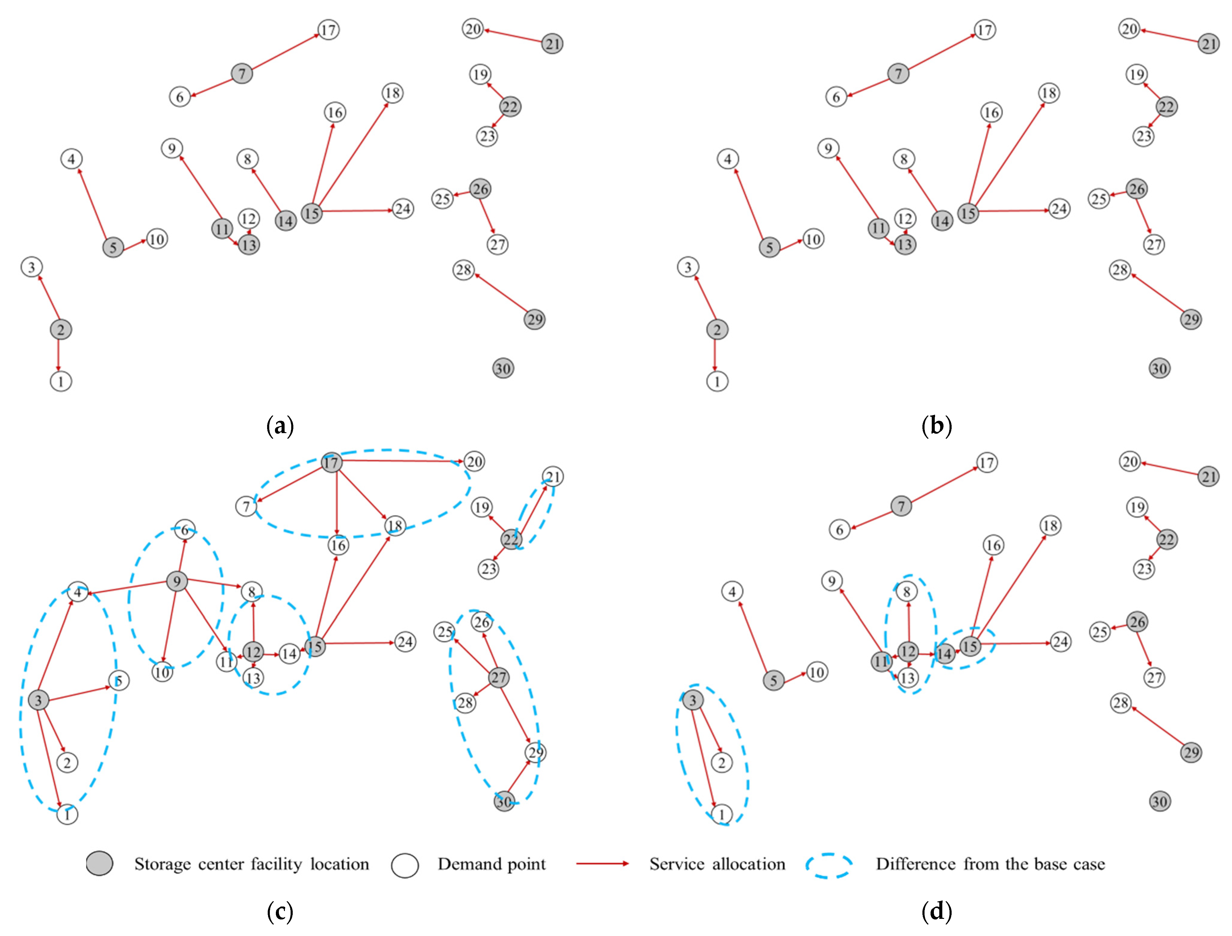
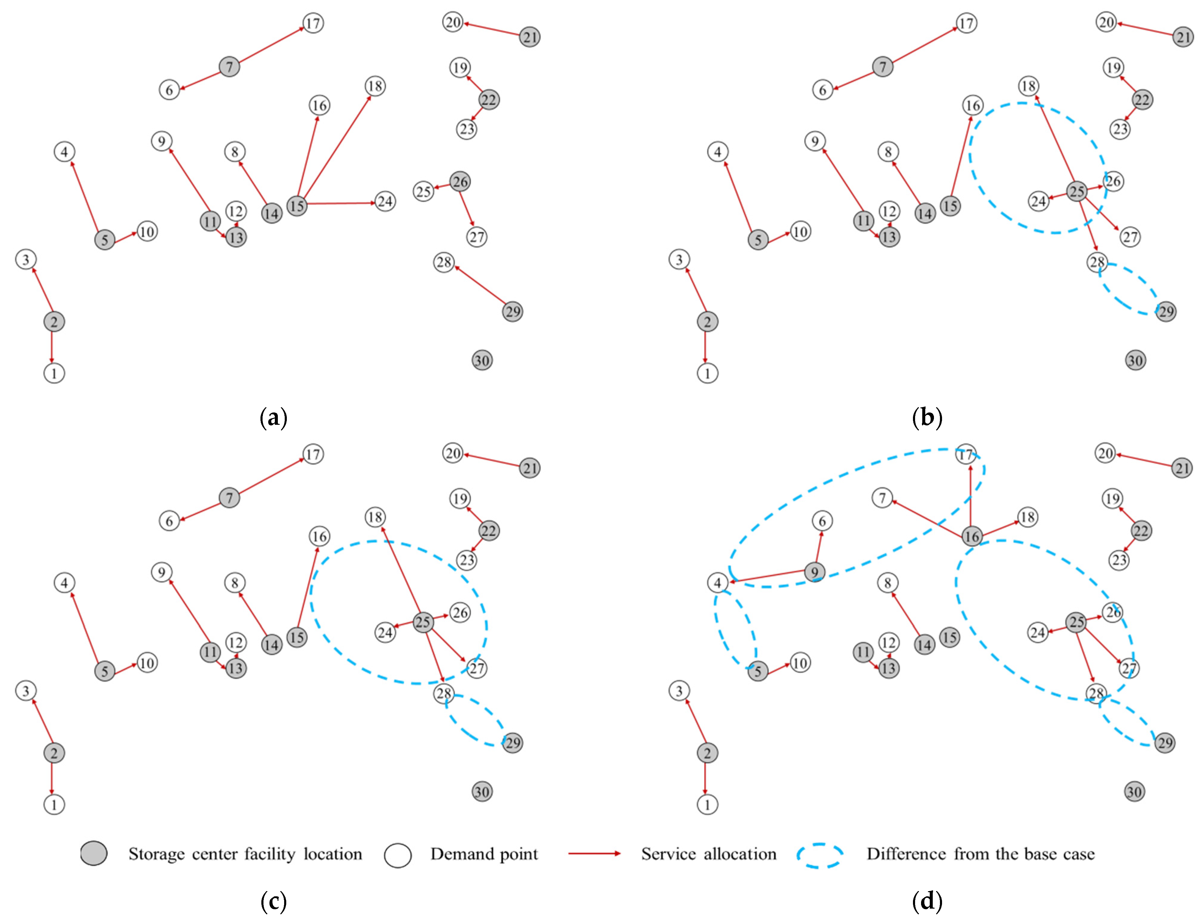
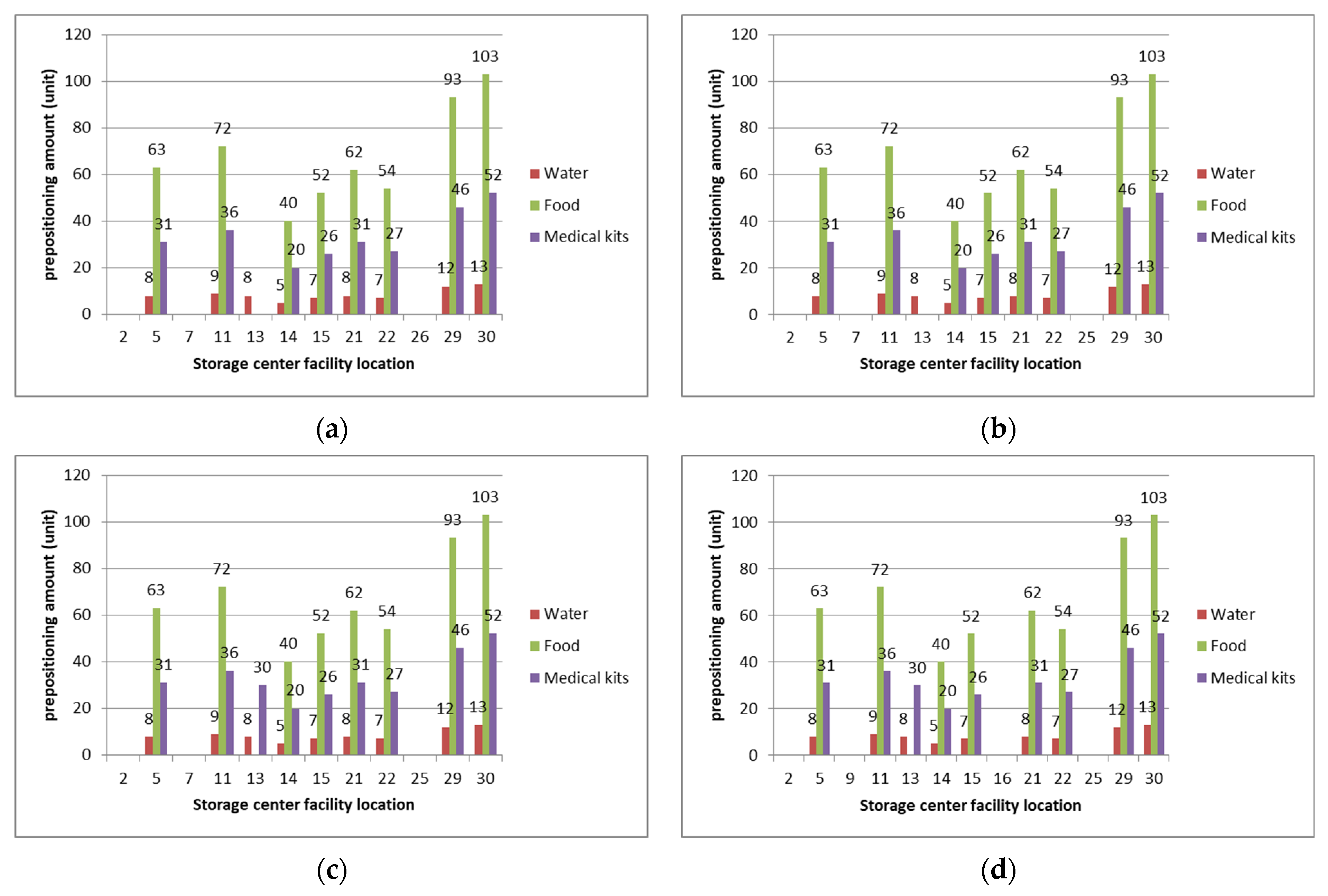
This section aims to test the effect of different deprivation cost functions on the optimal emergency logistics system design. The average case in the above section is used as the benchmark, where the traditional deprivation cost function, i.e., the form of exponential growth and linear hysteretic effect, is incorporated in the modeling structure. The other two forms of the deprivation cost functions are (1) exponential growth only and no hysteretic effect (Case I-1 and Case I-2) and (2) quadratic growth with linear hysteretic effect (Case II). The same parameter inputs were used in these models. In Case I, both t i j * = t i j and t i j * = 4   h were tested, where the former was used to make a direct comparison with the benchmark case on the hysteretic effect, and the latter is to examine the performance of a certain regular delivery pattern. According to Gutjahr and Fischer [29], if the commodity is food, the deprivation cost represents the increase in the victim’s hunger level with deprivation time. An example of the quadratic growth case is the function g ( t ) = 0.4 t 2 . On this basis, the coefficients in the quadratic deprivation cost function were assumed to be 0.6 for water, 0.4 for food, and 1.0 for a medical kit, respectively. Figure A3 and Figure A4 present the optimization results when considering the other two forms of the deprivation cost functions, and Table A2 shows the specific values of the cost components in all three cases.
It can be seen from the above results that there is no significant difference between the Benchmark case and Case I-1, i.e., when considering the same accumulation mode of deprivation cost and investigating the hysteretic effect, the hysteretic effect did not have a great impact on the key decisions of the system (e.g., facility location, service allocation, and even the amount of the prepositioned supplies) based on the results, even though the duration of a delivery cycle and the delivery frequency may change. The main reason is that it only changes the measurement method of the victims’ losses. As a result, it may produce different deprivation costs, but it is not enough to affect other key decisions.
When the transportation period of all disaster areas is fixed at a certain time value, such as 4 h, which can be understood as a unified fixed period transportation plan for disaster sites, and no hysteretic effect is considered (Case I-2), the location and allocation results shown in Figure A3c have changed a lot. The transportation period of the Benchmark case and Case I-1 may primarily depend on the travel time between storage center i to victim group j; it may be longer or shorter than four hours. However, when fixing all the delivery cycles to a certain value, one significant change is the sharp increase in the deprivation cost of victims, and some demand nodes have to accept the supports from multiple suppliers, e.g., nodes 4, 11, 16, 18, and 29. The fixed transportation cycle is a kind of transportation plan which is close to reality, no matter how far or near the disaster site is, to realize the fairness of emergency rescue. But in this context, the deprivation cost and travel cost increase a lot, which indicates that if the focus of the government is to alleviate the suffering of victims, the service pattern with a fixed delivery period is not the right option.
Quadratic growth is another accumulation form of deprivation cost, which essentially changes the calculation method of the deprivation cost in the system. As the curve of quadratic growth is much gentler than that of exponential growth with the existing parameter setting, its numerical result of the deprivation cost shows a great reduction. We would like to know whether different measurement methods of deprivation cost will have a significant impact on the optimization results of the system. When comparing the Benchmark case (Figure A3a) and Case II (Figure A3d), some of the changes can be seen in facility location and service allocation decisions, but the impact is not so great.

4.4. Numerical Results of Different Travel Modes

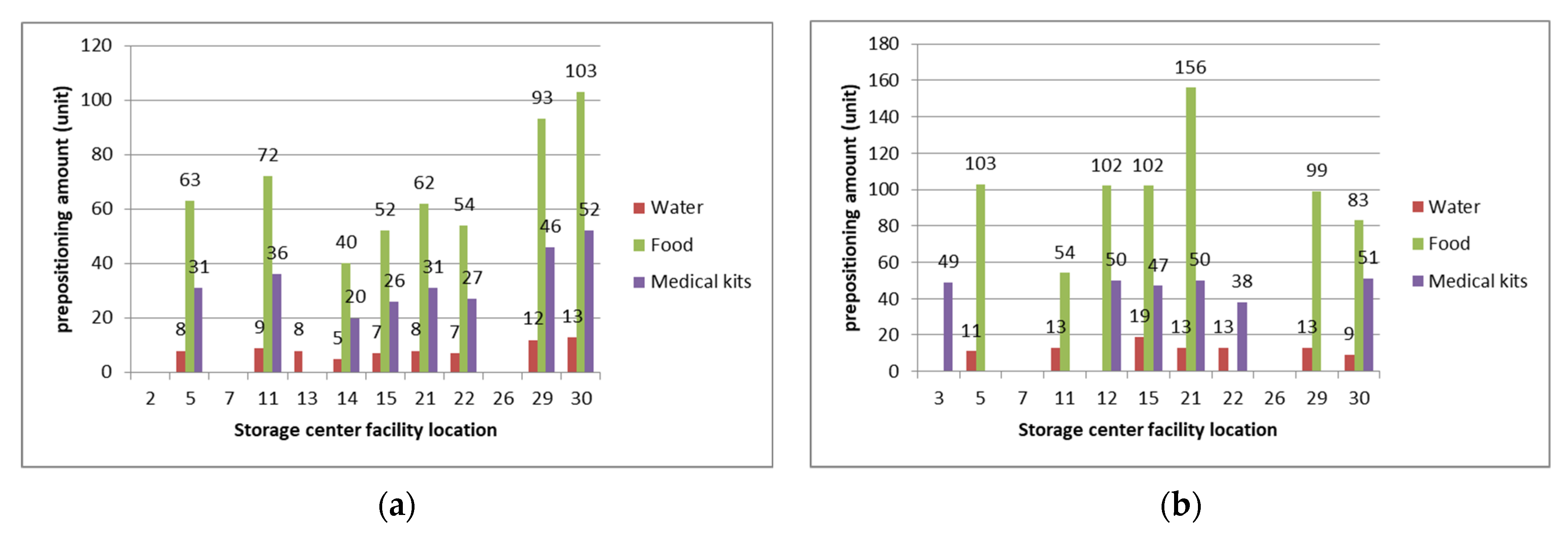
In some major disasters, the road infrastructure may be seriously damaged. In this case, it may not be able to transport relief materials by vehicle, but by aircraft. This paper also makes a comparative analysis of the effects of different transportation modes. The purpose is to check whether there will be significant changes in the layout of critical facility locations and service allocation plan at the strategic level when different transportation modes are adopted. Let us say that the speed of aircraft transportation is 800 miles per hour, and the same random demand distribution is used in comparative cases. When only aircraft transportation is considered, the model optimization results are shown in Figure A5 and Figure A6, and the related cost components are listed in Table A3.
When transportation becomes faster, the preset of materials will become more centralized. For example, in the case of vehicle transportation, almost every storage point reserves three types of materials, while in the case of aircraft transportation, some storage points may only reserve one or two types of materials, but the quantity is larger. Moreover, when adopting aircraft transportation, there are more service relationships established from the material storage point to the surrounding areas, even between the supply points, not just one-point to one-point services.
When aircraft transportation is used, the system transportation cost will be greatly increased, and even play an important role in the total cost (for example, the transportation cost is $2.99 in the case of aircraft transportation). However, after using aircraft transportation, the waiting time of victims for the arrival of materials can be considerably shortened, and the deprivation cost can be lowered in a large span. In this context, due to the improvement of transportation speed and service diversity, the location number of storage facilities shows a trend of decrease, and the total quantity of prepositioned materials also decreases due to centralized storage and distribution. As a result, the aircraft transportation mode shows a comparative advantage in total system cost. In practice, only using aircraft transportation may have some shortcomings such as high transportation costs and limited transportation volume. Therefore, according to the state of emergency, the mixed transportation mode of aircraft and vehicle will not only reduce the deprivation cost of victims and the total system cost but also improve the emergency response efficiency of the whole system.

4.5. Sensitivity Analysis

Above numerical results are obtained mostly based on determined values of transportation time between each node pair ( t i j ) and fixed coefficient value of deprivation cost ( β ), and these parameters may have a major impact on the optimal solutions. In this section, additional sensitivity analyses on these key inputs were carried out to examine their impacts on the model performance and draw managerial insights.
(1)
Transportation time
The increase in transportation time can be used to represent the increase in travel difficulty along the road networks. In this paper, the cumulative time of deprivation cost is defined as the travel times between origins and destinations. Therefore, if the travel time between network nodes rises, it directly reveals that the cumulative time of deprivation cost will go up, as well as the related deprivation cost. To balance all the cost components through optimization, as the four cases show in Figure A7 and Figure A8, the system will tend to build more optimal storage centers (e.g., from 12 to 13 optimal locations when comparing Figure A7a,d) in Table A4, and for those demand points with more/positive emergency demand, the system was inclined to contract their outward service to reduce the system travel cost.
(2)
Weighting coefficient
Coefficient β was used to characterize the decision maker’s propensity to victims’ interests in the decision-making process. In this section, a few coefficient values of β were input to test its sensitivity to the model’s optimization. Location and allocation results under β = 2 and β = 5 are shown in Figure A9 and Figure A10, and the numerical results are listed in Table A5.
When the interests of the victims in the process of system optimization are not going to be considered, i.e., β = 0 , the problem degenerates to the ordinary p-median problem. The optimization process is to balance the facility set-up cost, material prepositioning cost, and travel cost. Due to the lack of deprivation cost in the modeling structure, the number of optimal locations was reduced, but the travel cost increased greatly.
When taking into account the deprivation cost of the victims in the modeling framework (i.e., β > 0 ) with the increase of β based on the results, for example, from β = 1 to β = 5 , the decisions on the facility location, service allocation, and the preset quantity of materials did not change significantly, but the total number of optimal locations under each positive β value was far more than that of β = 0 . In other words, to reduce the deprivation cost of the victims to the greatest extent, the system tends to build more storage centers and the optimal locations are usually built locally or near the demand point. However, it was also proved that increasing the weight on the interests of the victims in the decision-making process was not so necessary. The outward service function of each location might gradually decrease (i.e., the service allocation relationship will decrease) with a bigger β , but for the key decisions across the whole system, there was not much change.

5. Conclusions

In the process of humanitarian relief, the priority of emergency activities is to reduce the losses suffered by the victims as much as possible. Prepositioning necessary emergency materials in disaster-prone areas before a disaster and providing emergency materials from the interests of victims after the disaster are both effective ways to realize this loss reduction. In this paper, these details were embedded into a scenario-based humanitarian logistics network design and service allocation modeling framework, and specifically, the deprivation cost function was used to characterize the victims’ losses when they were waiting for the emergency materials. The modeling strategy was to provide emergency storage facility location, material prepositioning, and service allocation decisions of each scenario in the same integrated modeling structure to minimize facility set-up cost, material handling cost, victims’ deprivation cost, and material transportation cost. Three typical forms of deprivation cost functions were considered: (1) exponential growth with linear hysteretic effect; (2) exponential growth only and no hysteretic effect; and (3) quadratic growth with linear hysteretic effect to examine the impact.
The same experimental road network in the Gulf Coast area of the US (Rawls and Turnquist [9]) was applied to test the performance of the proposed model. The numerical results show that no matter under what kind of demand situation, the deprivation cost occupies about 22–44% of the total cost, and it was indeed nonnegligible when making optimal decisions. Moreover, due to the additional considerations of the deprivation cost of victims in the modeling framework, the system tends to establish emergency storage centers locally and most of the service allocation relationships present simple one-to-one or one-to-two modes, to centralize the supply of relief materials and reduce the loss of victims to the greatest extent. When considering different levels of demand (e.g., when it is hard to estimate the exact emergency demand under disaster conditions), the facility location results are not very sensitive to the change of the demand values. When considering different forms of the deprivation cost function, it can be found that the change of the function form does not have a significant impact on the final optimal solutions, even if the measurement method of victims’ losses changes. However, if the periodical transportation mode is changed, for example, the service interval changes from separate travel time intervals to a unified fixed period, the system optimal solutions will change dramatically. It reflects the results of two different service allocation strategies in practice. Additionally, the sensitivity analysis results indicated that when (1) the travel time between network nodes and (2) the weight of the deprivation cost in the modeling framework increase (e.g., the transportation road network is damaged in the disaster and the travel time generally increase or the decision-maker put more focus on the victims’ benefits), more locations and more contracted service modes can be observed. The advantage of aircraft transportation mode was also testified through a comparative analysis.
This paper set the service interval for each victim group based on the travel time between the supply and demand nodes and tested the case with a fixed period in the numerical study, which might not be so flexible for disaster scenarios. Future research may attempt to explore the optimal service interval for each victim group to reach a better optimization. The attempt may add a higher nonlinear structure in the calculation of the deprivation cost based on the current exponential or quadratic formulations which will be more challenging. More efforts can also be directed towards the development of customized algorithms to solve such nonlinear problems. Furthermore, the integration of deprivation cost in other optimization problems of humanitarian logistics may be worthy of investigation.

Author Contributions

Conceptualization, methodology, programming, and numerical analysis, L.Z. and N.C.; writing—original draft preparation, L.Z. and N.C.; writing—review and editing, N.C.; project administration, N.C.; funding acquisition, N.C. All authors have read and agreed to the published version of the manuscript.

Funding

This research was funded by the National Natural Science Foundation of China (NSFC), grant number 71874069, and the Introduction and Cultivation Plan of Young Innovative Talents in Colleges and Universities of Shandong Province.

Institutional Review Board Statement

Not applicable.

Informed Consent Statement

Not applicable.

Data Availability Statement

The shape of the road network and the historical records of 15 hurricane events and 51 scenarios (including both separate events and joint events) used in the numerical experiments were cited from Rawls and Turnquist’s [9] study, which has been clearly stated in the manuscript.

Conflicts of Interest

The authors declare no conflict of interest.

Appendix A

Figure A1. Location and allocation relationship under four demand conditions: (a) average case (base case); (b) minimum case (minimum demand); (c) worst case (maximum demand); (d) random case (random demand).
Sustainability 13 04141 g0a1
Figure A2. Location and material preset under four demand conditions: (a) average case (base case); (b) minimum case (minimum demand); (c) worst case (maximum demand); (d) random case (random demand).
Sustainability 13 04141 g0a2aSustainability 13 04141 g0a2b
Figure A3. Location and allocation results with different deprivation cost functions. (a) Benchmark case (exponential growth with linear hysteretic effect); (b) Case I-1 (exponential growth only and no hysteretic effect, t i j * = t i j ); (c) Case I-2 (exponential growth only and no hysteretic effect, t i j * = 4   h ); (d) Case II (quadratic growth with linear hysteretic effect).
Sustainability 13 04141 g0a3
Figure A4. Location and material preset with different deprivation cost functions. (a) Benchmark case (exponential growth with linear hysteretic effect); (b) Case I-1 (exponential growth only and no hysteretic effect, t i j * = t i j ); (c) Case I-2 (exponential growth only and no hysteretic effect, t i j * = 4   h ); (d) Case II (quadratic growth with linear hysteretic effect).
Sustainability 13 04141 g0a4
Figure A5. The experimental results with different travel modes. (a) Location and service allocation in the case of vehicle transportation; (b) location and allocation in the case of aircraft transportation.
Sustainability 13 04141 g0a5
Figure A6. Location and material preset with different travel modes. (a) Location and service allocation in the case of vehicle transportation; (b) location and allocation in the case of aircraft transportation.
Sustainability 13 04141 g0a6
Figure A7. Results of different transportation time intervals. (a) Location and allocation under 1.2 times travel time; (b) location and allocation under 1.5 times travel time; (c) location and allocation under 1.8 times travel time; (d) location and allocation under 2 times travel time.
Sustainability 13 04141 g0a7
Figure A8. Location and material preset different transportation time intervals. (a) Location and allocation under 1.2 times travel time; (b) location and allocation under 1.5 times travel time; (c) location and allocation under 1.8 times travel time; (d) location and allocation under 2 times travel time.
Sustainability 13 04141 g0a8
Figure A9. The experimental results with different weighting coefficients. (a) Location and allocation under β = 2 ; (b) location and allocation under β = 5 .
Sustainability 13 04141 g0a9
Figure A10. Location and material preset with different weighting coefficients. (a) Location and allocation under β = 2 ; (b) location and allocation under β = 5 .
Sustainability 13 04141 g0a10
Table A1. Location results and cost components under three demand conditions.
CaseLocation Fixed   Cost   ( × 10 6 $ ) Handling   Cost   ( × 10 6 $ ) Travel   Cost   ( $ ) Deprivation   Cost   ( × 10 6 $ ) Total   Cost   ( × 10 6 $ )
Minimum demand2,5,7,11,13,14,15,21,22,26,29,301.991.163632.605.75
Average demand
(base case)
2,5,7,11,13,14,15,21,22,26,29,301.993.6915442.768.44
Maximum demand2,5,7,11,12,13,14,15,21,22,26,29,302.1910.173673.5215.81
Stochastic demand2,5,7,11,13,14,15,21,22,26,29,301.995.8417362.7910.62
Table A2. Location results and cost components with different deprivation cost functions.
CaseLocation Fixed   Cost   ( × 10 6 $ ) Handling   Cost   ( × 10 6 $ ) Travel   Cost   ( $ ) Deprivation   Cost   ( × 10 6 $ ) Total   Cost   ( × 10 6 $ )
Benchmark case (exponential growth with hysteretic effect)2,5,7,11,13,14,15,21,22,26,29,301.993.6915442.768.44
Case I-1 (exponential growth only and no hysteretic effect, t i j * = t i j )2,5,7,11,13,14,15,21,22,26,29,301.993.6915442.718.39
Case I-2 (exponential growth only and no hysteretic effect, t i j * = 4   h )3,9,12,15,17,22,27,301.363.2711,62840.845.43
Case II
(quadratic growth with linear hysteretic effect)
3,5,7,11,12,14,15,21,22,26,29,302.033.3623680.415.80
Table A3. Results under different transportation modes.
CasesLocation Fixed   Cost   ( × 10 6 $ ) Handling   Cost   ( × 10 6 $ ) Travel   Cost   ( $ ) Deprivation   Cost   ( × 10 6 $ ) Total   Cost   ( × 10 6 $ )
Vehicle transportation2,5,7,11,13,14,15,21,22,26,29,301.995.2718042.7810.04
Aircraft transportation3,5,7,11,12,15,21,22,26,29,301.863.782.990.348.97
Table A4. Comparison results under transportation time change.
CaseLocation Fixed   Cost   ( × 10 6 $ ) Handling   Cost   ( × 10 6 $ ) Travel Cost ($) Deprivation   Cost   ( × 10 6 $ ) Total   Cost   ( × 10 6 $ )
t i j
(Base case)
2,5,7,11,13,14,15,21,22,26,29,301.993.6915442.768.44
1.2 t i j 2,5,7,11,13,14,15,21,22,26,29,301.993.6915443.409.08
1.5 t i j 2,5,7,11,13,14,15,21,22,25,29,302.033.6915444.3810.10
1.8 t i j 2,5,7,11,13,14,15,21,22,25,29,302.034.0513505.0311.11
2 t i j 2,5,9,11,13,14,15,16,21,22,25,29,302.214.0513505.5811.84
Table A5. Results with different weight coefficients.
CasesLocation Fixed   Cost   ( × 10 6 $ ) Handling   Cost   ( × 10 6 $ ) Travel   Cost   ( $ ) Deprivation   Cost   ( × 10 6 $ ) Total   Cost   ( × 10 6 $ )
β = 5 2,5,7,11,13,14,15,21,22,25,29,302.034.06128313.0019.09
β = 2 2,5,7,11,13,14,15,21,22,26,29,301.993.6915445.5311.21
β = 1
(Base case)
2,5,7,11,13,14,15,21,22,26,29,301.993.6915442.768.44
β = 0 5,12,19,300.691.890.1702.75

References

  1. UNISDR. Hyogo Framework for Action 2005–2015 Building the Resilience of Nations and Communities to Disasters. In Proceedings of the World Conference on Disaster Reduction, Hyogo, Japan, 18–22 January 2005. [Google Scholar]
  2. Ni, W.; Shu, J.; Song, M. Location and Emergency Inventory Pre-Positioning for Disaster Response Operations: Min-Max Ro-bust Model and a Case Study of Yushu Earthquake. Prod. Oper. Manag. 2018, 27, 160–183. [Google Scholar] [CrossRef]
  3. Djimesah, I.E.; Okine, A.N.D.; Mireku, K.K. Influential factors in creating warning systems towards flood disaster management in Ghana: An analysis of 2007 Northern flood. Int. J. Disaster Risk Reduct. 2018, 28, 318–326. [Google Scholar] [CrossRef]
  4. Thomas, A. Humanitarian Logistics Enabling Disaster Response; Fritz Institute: San Francisco, CA, USA, 2004. [Google Scholar]
  5. Pérez-Rodríguez, N.; Holguín-Veras, J. Inventory-Allocation Distribution Models for Postdisaster Humanitarian Logistics with Explicit Consideration of Deprivation Costs. Transp. Sci. 2016, 50, 1261–1285. [Google Scholar] [CrossRef]
  6. Holguín-Veras, J.; Jaller, M.; Van Wassenhove, L.N.; Pérez, N.; Wachtendorf, T. On the unique features of post-disaster humani-tarian logistics. J. Oper. Manag. 2012, 30, 494–506. [Google Scholar] [CrossRef]
  7. McLachlin, R.; Larson, P.D.; Khan, S. Not-for-profit Supply Chains in Interrupted Environments The Case of a Faith-based Humanitarian Relief Organisation. Manag. Res. News 2009, 32, 1050–1064. [Google Scholar] [CrossRef]
  8. Holguín-Veras, J.; Jaller, M. Immediate Resource Requirements after Hurricane Katrina. Nat. Hazards Rev. 2012, 13, 117–131. [Google Scholar] [CrossRef]
  9. Rawls, C.G.; Turnquist, M.A. Pre-positioning of emergency supplies for disaster response. Transp. Res. Part B Methodol. 2010, 44, 521–534. [Google Scholar] [CrossRef] [Green Version]
  10. Besiou, M.; Stapleton, O.; Van Wassenhove, L.N. System dynamics for humanitarian operations. J. Humanit. Logist. Supply Chain Manag. 2011, 1, 78–103. [Google Scholar] [CrossRef]
  11. Khayal, D.; Pradhananga, R.; Pokharel, S.; Mutlu, F. A model for planning locations of temporary distribution facilities for emergency response. Socio-Econ. Plan. Sci. 2015, 52, 22–30. [Google Scholar] [CrossRef]
  12. Moreno, A.; Alem, D.; Ferreira, D.; Clark, A. An effective two-stage stochastic multi-trip location-transportation model with social concerns in relief supply chains. Eur. J. Oper. Res. 2018, 269, 1050–1071. [Google Scholar] [CrossRef] [Green Version]
  13. Khorram-Manesh, A.; Phattharapornjaroen, P.; Mortelmans, L.J.; Goniewicz, K.; Verheul, M.; Sörensen, J.L.; Pereira, I.; Ricklin, M.; Faccincani, R.; Dark, P.M.; et al. Current Perspectives and Concerns Facing Hospital Evacuation: The Results of a Pilot Study and Literature Review. Disaster Med. Public Health Prep. 2021, 1–9. [Google Scholar] [CrossRef]
  14. Holguín-Veras, J.; Pérez, N.; Jaller, M.; Van Wassenhove, L.N.; Aros-Vera, F. On the appropriate objective function for post-disaster humanitarian logistics models. J. Oper. Manag. 2013, 31, 262–280. [Google Scholar] [CrossRef]
  15. Holguín-Veras, J.; Amaya-Leal, J.; Cantillo, V.; Van Wassenhove, L.N.; Aros-Vera, F.; Jaller, M. Econometric estimation of depriva-tion cost functions: A contingent valuation experiment. J. Oper. Manag. 2016, 45, 44–56. [Google Scholar] [CrossRef]
  16. Cantillo, V.; Serrano, I.; Macea, L.F.; Holguín-Veras, J. Discrete choice approach for assessing deprivation cost in humanitarian relief operations. Socio-Econ. Plan. Sci. 2018, 63, 33–46. [Google Scholar] [CrossRef]
  17. Cotes, N.; Cantillo, V. Including deprivation costs in facility location models for humanitarian relief logistics. Socio-Econ. Plan. Sci. 2019, 65, 89–100. [Google Scholar] [CrossRef]
  18. Zhu, L.; Gong, Y.; Xu, Y.; Gu, J. Emergency relief routing models for injured victims considering equity and priority. Ann. Oper. Res. 2018, 283, 1573–1606. [Google Scholar] [CrossRef]
  19. Shao, J.; Wang, X.; Liang, C.; Holguín-Veras, J. Research progress on deprivation costs in humanitarian logistics. Int. J. Disaster Risk Reduct. 2020, 42, 101343. [Google Scholar] [CrossRef]
  20. An, S.; Cui, N.; Li, X.; Ouyang, Y. Location planning for transit-based evacuation under the risk of service disruptions. Transp. Res. Part B Methodol. 2013, 54, 1–16. [Google Scholar] [CrossRef]
  21. Yu, L.; Zhang, C.; Yang, H.; Miao, L. Novel methods for resource allocation in humanitarian logistics considering human suf-fering. Comput. Ind. Eng. 2018, 119, 1–20. [Google Scholar] [CrossRef]
  22. MacPherson, R.I.; Burkle, F.M. Humanitarian Aid Workers: The Forgotten First Responders. Prehospital Disaster Med. 2021, 36, 111–114. [Google Scholar] [CrossRef] [PubMed]
  23. Sheu, J.-B. An emergency logistics distribution approach for quick response to urgent relief demand in disasters. Transp. Res. Part E Logist. Transp. Rev. 2007, 43, 687–709. [Google Scholar] [CrossRef]
  24. Oliva, S.; Lazzeretti, L. Measuring the economic resilience of natural disasters: An analysis of major earthquakes in Japan. City Cult. Soc. 2018, 15, 53–59. [Google Scholar] [CrossRef]
  25. IFIS. The International Federation’s Global Agenda (2006–2010); International Federation of Red Cross and Red Crescent Societies: Paris, France, 2006. [Google Scholar]
  26. Barmania, S. Typhoon Haiyan recovery: Progress and challenges. Lancet 2014, 383, 1197–1199. [Google Scholar] [CrossRef]
  27. IFRC. World Disasters Report, 2015: Focus on Local Actors, the Key to Humanitarian Effectiveness; International Federation of Red Cross and Red Crescent Societies: Paris, France, 2016. [Google Scholar]
  28. Rattanakanlaya, K.; Sukonthasarn, A.; Wangsrikhun, S.; Chanprasit, C. A survey of flood disaster preparedness among hospitals in the central region of Thailand. Australas. Emerg. Nurs. J. 2016, 19, 191–197. [Google Scholar] [CrossRef] [PubMed]
  29. Gutjahr, W.J.; Fischer, S. Equity and deprivation costs in humanitarian logistics. Eur. J. Oper. Res. 2018, 270, 185–197. [Google Scholar] [CrossRef]
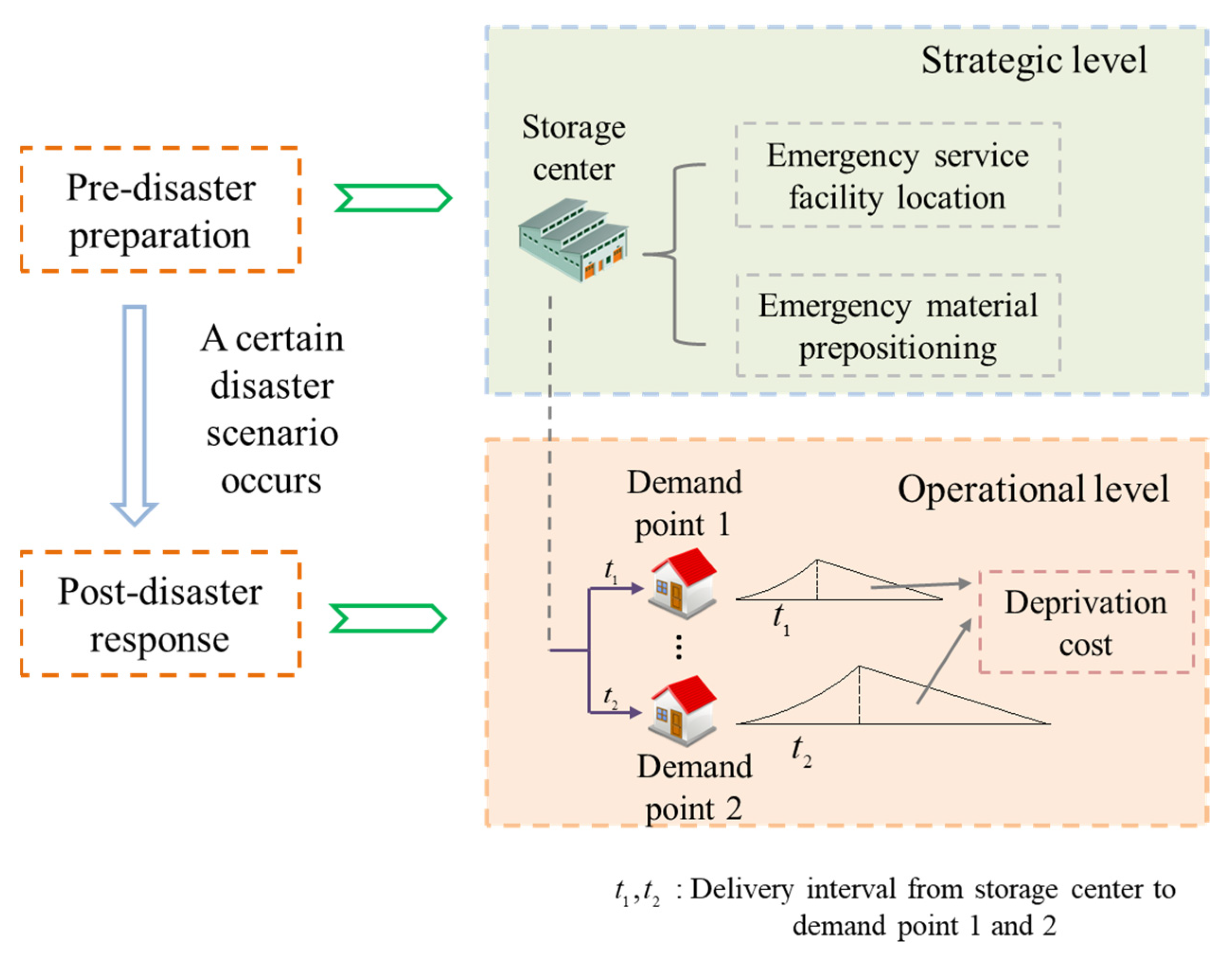
Figure 1. The modeling framework for both strategic and operational levels.
Sustainability 13 04141 g001
Figure 2. The allocation mode from storage centers to demand points.
Sustainability 13 04141 g002
Figure 3. The curve of the deprivation cost at the demand point over time.
Sustainability 13 04141 g003
Figure 4. The curve of the deprivation cost without hysteresis effect.
Sustainability 13 04141 g004
Figure 5. The curve of the deprivation cost with the quadratic accumulation form.
Sustainability 13 04141 g005
Table 1. Unit storage space, consumption rate, transportation cost, and link flow of commodities (per unit).
Commodities η k ( f t 3 ) ρ k ( f t 3 ) c i j k s ( $ / mile )
Water (1000 gals)144.60.000440.45
Food (1000 MREs)83.330.0030.112
Medical kits (1000)11600.0010.66
MRE: meals-ready-to-eat.
Table 2. Hurricanes, affected nodes, and population of each demand point ( P j ).
HurricaneAffected NodePopulation
156132
2143929
3225274
4225274
5117081
299100
6155105
7216052
8117081
9135936
299100
10216052
11216052
12155105
13299100
14143929
3010,120
15225274
Table 3. The coefficients of the deprivation cost function.
Commodities a k b k
Water0.11721.5031
Food0.11.2
Medical kits0.672
Publisher’s Note: MDPI stays neutral with regard to jurisdictional claims in published maps and institutional affiliations.