More from Less? Environmental Rebound Effects of City Size

Abstract

Global sustainability relies on our capacity of understanding and guiding urban systems and their metabolism adequately. It has been proposed that bigger and denser cities are more resource-efficient than smaller ones because they tend to demand less infrastructure, consume less fuel for transportation and less energy for cooling/heating in per capita terms. This hypothesis is also called Brand’s Law. However, as cities get bigger, denser and more resource-efficient, they also get richer, and richer inhabitants consume more, potentially increasing resource demand and associated environmental impacts. In this paper, we propose a method based on scaling theory to assess Brand’s Law taking into account greenhouse gas (GHG) emissions from both direct (energy and fuels locally consumed) and indirect (embedded in goods and services) sources, measured as carbon footprint (CF). We aim at understanding whether Brand’s Law can be confirmed once we adopt a consumption-based approach to urban emissions. By analyzing the balance between direct and indirect emissions in a theoretical urban system, we develop a scaling theory relating carbon footprint and city size. Facing the lack of empirical data on consumption-based emissions for cities, we developed a model to derive emission estimations using well-established urban metrics (city size, density, infrastructure, wealth). Our results show that, once consumption-based CF is considered, Brand’s Law falls apart, as bigger cities have greater purchase power, leading to greater consumption of goods and higher associated GHG. Findings also suggest that a shift in consumption patterns is of utmost importance, given that, according to the model, each new monetary unit added to the gross domestic product (GDP) or to other income variables results in a more than proportional increase in GHG emissions. This work contributes to a broader assessment of the causes of emissions and the paradigm shift regarding the assumption of efficiency in the relationship of city size and emissions, adding consumption behavior as a critical variable, beyond Brand’s Law.

1. Introduction

We live in a predominantly urban world, and rural to urban migration is not showing signs of slowing down. With population growth, the urban metabolism—all the exchanges between the city and the environment—is modified in diverse ways and we can expect challenges emerging in the management of, among others, environmental impacts, resource consumption and waste disposal. Cities devour about 70% of resources, and consume 80% of the energy worldwide [1]. It has become clear that global sustainability relies on our capacity of understanding and guiding urban systems and their metabolism adequately.

Strong is the faith in the dense city. Urban density is well-established as a solution to sustainability in cities [2,3] to the point of being identified by the Intergovernmental Panel on Climate Change (IPCC) as a crucial climate mitigation measure [4]. It is frequently argued that dense cities are more sustainable than sparse ones. As there is conclusive empirical evidence that density increases with population size [5,6,7], it has been proposed that bigger cities are also more resource-efficient than smaller ones [8]. This hypothesis—“As cities get bigger, they also get greener”—is called Brand’s Law. It stands for the fact that bigger and denser human settlements tend to demand less infrastructure per capita [9], less fuel consumption for transportation [10] and less energy consumption for cooling/heating [11]. Apparently, bigger cities do more with less [12].

“But a city is more than a place in space, it is a drama in time” [13]. Cities are not only the space they fill or the infrastructure they use for it. Cities are their social interactions as well. Recent theoretical works [14,15,16,17] have shown that the interaction between people is one of the main drivers of economic activity and wealth creation (see also [18,19,20]). As cities get bigger, they also get more than proportionally productive and richer. Richer inhabitants buy more, increasing their resource demand and associated environmental impacts.

To fully understand the nexus between city size or density and the environmental impacts generated by a city, we need to take into account greenhouse gas (GHG) emissions from both direct (energy and fuels locally consumed) and indirect (embedded in goods and services) sources. As urban agglomerations heavily rely on the supply of goods from outside their physical barriers, a consumption approach built on a life cycle perspective has been recommended by many specialists [21,22,23]. For the case of urban GHG emissions, there has been a gradual change from the first accounting protocols focusing on territorial production-based emissions to protocols accounting for upstream impacts of key materials and energy. More recently, this shift has included protocols accounting for emissions embedded in upstream flows and goods consumed by the city [24]. Figure 1, based on Chen et al. [24], visually describes the differences between GHG accounting methods commonly found in the literature and their relation to the IPCC’s “scope 1–3” concept [25,26]. While Territorial Emissions (TE) only account for emissions from sources within the city’s boundary (scope 1), Community-wide infrastructure-based carbon footprint (CIF) also includes emissions embodied in key items like energy, water and building materials (scope 2). Consumption-based carbon footprint (CF) adds to the previous emissions embodied in imports but deducts emissions embodied in exports.

In this paper, we will adopt the carbon footprint as the accounting method to understand the environmental impacts of cities. As a result of the novelty of the carbon footprint approach, the lack of empirical data and complexity of the analysis, studies using a consumption-based approach generally (i) focus on individual cases [27,28]; and (ii) rely either on sample survey data or scaled-down data from national accounts [29,30,31,32,33]. Up to now, findings indicate that consumption-based emissions are substantially greater than production-based ones [22], and that denser/bigger cities have proportionally less direct emissions (energy/fuels locally consumed) but greater indirect emissions (embedded in goods and services) than smaller ones [29,30,31,32,33]. However, due to the limited number of cases, the relationship between population size and total emissions (CF) remains unclear.

We propose a mean-field model to derive emission estimations out of well-established urban metrics (namely, city size, density, infrastructure, wealth). We expect the stylized model to enable us to better understand the relationship between population size and environmental impacts in cities. In order to do so, we articulate both aspects of the problem at a broad theoretical level, as a toy model. We want to understand if Brand’s Law holds true after adopting a consumption-based approach to urban emissions. In short, we wish to develop and test a theory of scaling between consumption-based carbon footprint and city size, taking into account the balance between direct and indirect emissions in a theoretical urban system. The main objective of the model is to identify potential real-world situations where Brand’s Law may lose validity. Our results will show that, on the one hand, when only territorial-based emissions are considered, bigger cities are greener as the law predicts. However, when taking into account consumption-based emissions, our model suggests that bigger cities have a greater total volume of GHG (direct plus indirect) emissions. In fact, each new monetary unit added to the GDP—or any other income variable—results in a more than proportional increase in GHG emissions. We argue that this is the case because a higher purchasing power leads to greater consumption of goods. In that scenario, Brand’s Law falls apart.

The paper is organized as follows. In Section 2, we present briefly the ideas behind urban scaling theory addressing how certain infrastructure and socio-economic metrics behave according to the city population size. In Section 3, we discuss how the environment is affected by the size, density, income and infrastructure of cities. In Section 4, we propose a model that takes into account direct and indirect emissions using well-established urban metrics (city size, density, infrastructure, wealth). Results of this model are discussed in Section 5, including scenarios where Brand’s Law cannot be confirmed. Finally, the main implications of our findings are presented in the conclusion Section 6.

2. Urban Scaling

We mentioned a lack of empirical data on the relationship between city size and environmental impacts. Quite differently, scientific evidences on the relationship between city size, infrastructure demand and wealth creation seem to be increasingly robust, unfolding into the so called new science of cities (NSC) [8,34,35]. The NSC involves a growing set of theoretical and quantitative approaches based on urban data and models to systematically understand urban phenomena [6,35,36,37]. One of the main pillars of this new science is the proposition that urban systems display universal scaling behavior regarding socioeconomic, infrastructural and individual services [15]. In the last decade, several studies reported that some urban variables, say Y, systematically scale on a non-linear way with population N for different urban systems [15,38,39,40,41,42,43]. More specifically, the relation between Y and N assumes the form

$$Y=Y_0{N}^{\beta },$$

(1)

where $Y_0$, the intercept, and $\beta$, the scaling exponent, are specific parameters associated with a given urban variable. Empirical evidence shows that the value assumed by $\beta$ is strongly related to the urban variable category [43]. For instance, socio-economic variables, as GDP, total wages, number of patents, number of infectious diseases, among others, present $\beta >1$, namely a super-linear regime. That means that greater cities also have a greater per-capita ($Y/N$) socio-economic activity. Indeed, the empirical finds suggest $\beta \approx 1.15$ for socio-economic variables, implying that when a given city is two times bigger than another, the per-capita socio-economic quantities of this bigger city are, on average, 15% bigger—the so-called increasing returns to scale [16,17,43,44]. These numbers are robust and consistent even for countries entirely different in terms of economy, history and culture. The main explanation for this non-linear scaling is that socio-economic variables are a direct consequence of the number of interactions between the people, and this number grows super-linearly with the size of cities, as some theoretical propositions and empirical findings suggest [16,17,45]. Cities are the primary sites of social interaction, a condition for creativity and economic production [20]. Summarizing, one can say that interactions increase more than proportionally as cities grow.

In contrast, infrastructure variables such as urbanized area, total electrical cables length, total street length, gasoline consumption, number of petrol stations and number of schools, among others [15,43,46], present $\beta <1$, or a sub-linear regime. It means that larger cities require less infrastructure per-capita ($Y/N$). Indeed, empirical findings suggest $\beta \approx 0.85$ for infrastructure variables, implying that when a given city is two times bigger than another, the per-capita infrastructure quantities of this bigger city are, on average, 15% smaller. Like the case of socio-economic variables, these numbers are robust for different countries. Some theoretical models explain the urbanized area sub-linear behavior as a consequence of densification processes [16], and the sublinear number of amenities (number of petrol stations, etc.) as a consequence of supply and demand processes [17]. The observed patterns indicate that as cities get bigger, they foster human interactions, producing more social outputs with less infrastructural demand per capita. Summarizing, one can say that larger cities do more with less.

Finally, there is a third kind of urban variable, usually associated with individual needs, that scales linearly with population, that is $\beta =1$ [15]. Examples of such variables are the number of households and household water consumption [43]. The fact that the values of such exponents are nearly the same, showing similar behavior for different urban variables and different countries, suggests a potential universality in urban scaling [15,16,17,43,46,47], being also observed in the dynamic growth of individual cities [46,48]. Moreover, some theoretical works [16,17,49] suggest that socio-economic and infrastructure scaling exponents are in fact interrelated, in a way that $\beta =1+\delta$ for socio-economic variables, and $\beta =1-\delta$ for infrastructure variables, where $\delta \approx 0.15$ (obtained empirically) is the parameter that establishes an interrelation between these two regimes. In contrast to the large amount of works that have argued in favor of universality, a growing number of studies report deviations from the scaling hypothesis. For instance, exponents appear to be highly sensitive to the geographical and statistical definition of “city” [50,51], the adopted methods of estimation [52] and external factors such as macroeconomic structures [43,53] or governmental policies [54].

In the next section, we shall expand our discussion of urban scaling laws and the properties and deviations from universality into the critical variables of environmental impact, particularly those related to direct and indirect emissions.

3. On the Relation between City Size and Environmental Impacts

We explore in this section a number of empirical findings on the relations between city size, population density, income, infrastructure and environmental impacts. We will bring together evidences stemming from urban scaling approaches, and progressively relate them to the problem of environmental impacts, culminating in a synthetic ’causal diagram’ connecting the main factors highlighted by these approaches. The stylized facts found in such relations will be further explored in the construction of our model.

3.1. City Size and Density

Some studies have used urban scaling theory to relate population size and urban density through the scaling exponent of area, normally found to be smaller than 1 (sublinear) [16,55]. Works presenting empirical evidences found sublinear exponents between different area definitions and population size. Regarding the Global North, Bettencourt and Lobo [38] found values between 0.85 and 0.95 for four European urban systems (UK, Italy, Germany and France) as well as for Europe as a single urban system. Regarding the Global South, Adhikari and Beurs [42] found scaling exponents between 0.5 and 0.8 in different years for African cities, while Meirelles et al. [43] found an exponent of 0.84 for the Brazilian urban system. Regarding ancient urban systems, Cesaretti et al. [56] analyzed 173 medieval European settlements and found exponents close to $\frac{5}{6}$, while Ortman et al. [39] found values close to $\frac{2}{3}$ and $\frac{5}{6}$ for pre-Hispanic settlements in the Americas. There are still other works reporting sublinear scaling exponents between urban area and population [57,58,59]. Others studies, however, found counterexamples: Bettencourt and Lobo [38] found that the urbanized area scaled superlinearly with population in Spain; Cottineau et al. [60] found the exponent to be sensitive depending on the definition of city adopted in the scaling, with most values ranging in the sublinear spectra, but some revealed to be linear or superlinear. This sensitivity has also been analyzed and evidenced by Arcaute et al. [50].

The diversity of works spanning from developed and developing countries to ancient as well as modern urban systems suggests that the population-density relation is universal to cities and is not related to contemporary dynamics or local specificity. Even considering pieces of evidence defying this claim [61,62,63,64], the great majority of findings seems to support the proposition that bigger cities are denser. This proposition is also supported by empirical results found through other methods [5].

3.2. City Size and Income

Economic growth happens almost naturally with urbanization through agglomeration effects and increasing returns to scale [44]. Clustered people and businesses experience (i) a higher probability of interactions and (ii) the combination of diverse capabilities since larger numbers of people in a given area are likely to increase the diversity of demands, abilities and ideas [65]. These alone are already a source of economic growth [20,66], and by reducing the distance between people, agglomeration also allows energy and time savings [19,67] which foment those interactions. This implies that as cities get bigger, they get richer.

Various empirical evidences support the claim that cities produce economic development and wealth. Among the urban scaling publications, many authors have shown superlinear relations between population and GDP, with an expected exponent of 1.15 (or $\frac{7}{6}$) [16,17]. Empirical evidence has been found for China [15,16], Europe and European countries [38,50,68], Brazil [43,69] and the United States [36], among others, corroborating the superlinear relationship. Other economics-related variables also scale superlinearly with population, such as different aspects of income [16,69], wages [15,70] and expenditure [71]. On the other hand, Strano and Sood [53] found that although for European low-income cities the gross metropolitan product (GMP) scales superlinearly with population, for high-income cities it scales linearly, suggesting that from a certain stage of development, the GDP starts growing proportionally to the population. Arcaute et al. [50] found similar results for 535 cities in the UK, as did Bettencourt and West [36] for personal income in the US.

3.3. City Size and Infrastructure

We have seen that urban infrastructure tends to get more efficient as the city grows, and therefore, its variables in general scale sublinearly with population size. They are expected to scale with an exponent 0.85 (or $\frac{5}{6}$) [16], as originally supported by empirical evidence found for the length of electrical cables and road surface in Germany [15]. Other studies found similar results for other urban systems: Kuhnert et al. [72] for the length of low-voltage cables in Germany and the number of petrol stations in France, Germany, the Netherlands and Spain; Meirelles et al. [43,46] for the length of street, water supply networks and the number of primary and secondary schools in Brazil; Bettencourt [16] for impervious surfaces in the world and in the EU, built area in China, area of roads in the USA and Germany and length of pipes in Japan, among others. These data point towards the universality of urban infrastructure variables scaling sublinearly with population. This relation indicates that bigger cities should have smaller material demand per capita for infrastructure.

However, infrastructure variables vary a great deal. The heterogeneity of processes governing such variables makes it hard to assess their impacts categorically since they function and grow in significantly different ways. Following the scaling literature, they may be categorized into urban infrastructure (such as the number of gas stations, hospitals, total length of water and gas pipelines, roads, etc.) and household infrastructure (or individual basic services, such as number of houses, number of bathrooms or bedrooms per house, etc.). Studies have shown that infrastructure related to individual needs tend to scale linearly with population [15,43,50,69]. In spite of that, Schlapfer et al. [73] found that average building heights increase with population size, leading to a smaller surface-to-volume ratio in bigger cities, which implies that even if the number of household scales linearly with population, the resulting material and energy demand and their related environmental impacts probably increase sublinearly.

3.4. City Size and Emissions

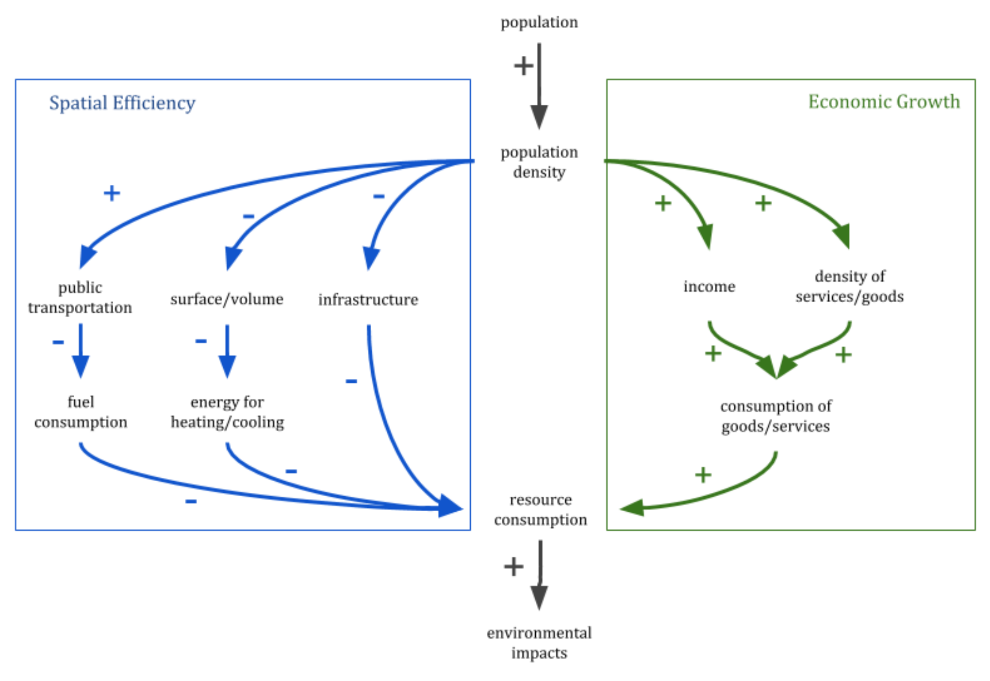
To the best of our knowledge, so far there has been no scientific consensus on the scaling regime of carbon footprint (CF) with population. In fact, due to limited data availability, most urban scaling studies consider only production-based emissions, hindering our capacity to analyze the total CF and its relationship with population size. Fragkias et al. [74] conducted several different analyses on a data set spanning ten years for approximately a thousand core-based statistical areas in the US (366 MSAs and 576 Micropolitan Areas) and found nearly-linear relationships in every case, with coefficients ranging from 0.9 to 0.95. The authors conclude that such findings refute the hypothesis that urban systems function similarly to biological ones, where the efficiency-size relationship is remarkably sublinear. Oliveira et al. [75] used remote sensing data to estimate production-based emissions from gridded data using 2281 clusters developed through a city clustering algorithm over the entire US territory and found that ${\mathrm{CO}}_2$ emissions scaled superlinearly with population with an average coefficient of 1.46. Even though the study did not consider consumption-based emissions, these results indicate that as population increases, cities become more polluted. Bettencourt and Lobo [38] also found a superlinear relation between ${\mathrm{CO}}_2$ emissions and population for 102 European Metropolitan areas with an exponent of 1.12, close to the value predicted by scaling theory (of $\frac{7}{6}$). Whatever the method of assessment, the estimation of ${\mathrm{CO}}_2$ emissions seems still problematic, and it is not possible to clearly identify whether the emissions are consumption or production-based. In this sense, Gudipudi et al. [76] explored four different sources for ${\mathrm{CO}}_2$ emissions data, mostly estimations based on production. On top of that, a small number of urban agglomerations from different countries were mixed to produce their results, indicating a lack of geographic consistency (scale analysis are expected to be performed within one single urban system). They found a superlinear relationship between ${\mathrm{CO}}_2$ emissions and population size for cities in Non-Annex I countries (i.e., countries outside the United Nations Framework Convention on Climate Change) ($\beta$ = 1.18) and a sublinear relationship for cities in Annex I countries ($\beta$ = 0.87).

Regardless of the results, all scaling studies lack consistent and harmonized consumption-based ${\mathrm{CO}}_2$ emissions data to properly analyze the cities’ carbon footprint, being the emissions usually estimated from production-based data alone. Problems emerging from data are closely related to methodological issues, making it impossible to reach a solid conclusion on how the total ${\mathrm{CO}}_2$ emissions scale with population and therefore, to know whether bigger cities are greener or not. A production-based figure is unable to differentiate between reduction and outsourcing of emissions in cities. Furthermore, the definition of city to be considered in each scaling greatly influences the resulting exponent. Louf and Barthelemy [51] demonstrated that adopting two different definitions of cities by the Census Bureau in the US resulted in completely different scaling results (from $\beta$ = 0.95 to $\beta$ = 1.37, implying that larger cities can be either greener or less green, respectively), an idea previously depicted for other urban variables [50,60]. Gudipudi et al. [77] also point out two other significant problems in scaling data: the spatial resolution, and the regression method adopted, which can also change the results of a study. In short, the methodological inconsistencies among urban emission scaling studies, lack of data on consumption-based GHG emissions and the absence of a solid theoretical background prevent these conclusions from being extrapolated to other urban realities or reaching general theoretical definitions.

Studies analyzing the relation between urbanization and consumption-based emissions are performed with methodologies other than scaling. The majority of these studies-carried out specially in cities in developed countries-lead to the conclusion that direct emissions tend to decrease with greater populations, whereas indirect emissions tend to increase with greater populations. The relation between total emissions and population is defined by the intensity of direct emissions savings and indirect emissions increase and is country-dependent. Pang et al. [78] analyzed the difference in emission patterns between rural and urban areas in Switzerland and found that direct emissions from urban areas were around 20% smaller than from rural ones, while indirect emissions were 5–10% higher making the total emission in urban areas smaller than in rural ones. Gill and Moeller [30] analyzed agglomerations in Germany classified by population ranges and found that the bigger the population, the lower the direct emissions per capita and the greater the indirect emissions, leading to a slight decrease of total emissions in bigger cities. Minx et al. [29] found that scope 1 and 2 emissions (emissions from withing city boundaries, and community-wide infrastructure-based CF, respectively) in England decreased from rural to urban areas, while scope 3 (emissions related to imported goods and services) increased, leading to constant total emissions per capita across the rural-to-urban range. Wiedenhofer et al. [79] found that urban households require less direct energy, but their total consumption is higher in Australia due to a big increase in indirect energy consumption. Heinonen et al. [80] found that emissions from housing and transportation decrease for bigger and denser settlements in Finland, but indirect emissions more than overcome that trend leading to greater overall emissions.

A report by the IPCC [81] states that, although limited, evidence suggests a higher consumption-based emission pattern in large cities than in rural areas for non-Annex I countries, with inconclusive results for Annex I countries. Furthermore, considering energy-related emissions (scope 2), the results are different for cities in Annex I and non-Annex I countries. Whilst two-thirds of the first show a lower per capita final energy use in comparison to their national averages, over two-thirds of the latter show the opposite result, indicating that the stage of development of the urban system greatly influences its emission patterns. Properly exploring this data and well-defining production and consumption-based emissions are fundamental steps to adequately analyze the total CF of urban cities in comparison to rural areas and their national averages, and reach more solid conclusions.

In turn, a recent study estimated consumption-based emissions (carbon footprints) for 13,000 cities across the globe (Gridded Global Model of City Footprints—GGMCF) [82]. To reach such estimations, authors down-scaled national CFs and added existing sub-national CF studies. The process of down-scaling assumes that household expenditure profiles are constant for different city sizes. This is unlikely to be the case and invalidates any study trying to understand the effect of city size on CF using the database. A closer look into the GGMCF data points to such complexities. Figure 2-left presents a histogram of scaling exponent ($\beta$) between population and carbon footprint for 27 countries using the GGMCF data [82] and the relationship between these $\beta$′s and the GDP of such countries. We estimated $\beta$ for all countries with more than three cities in the GGMCF database. Differently from other variables, $\beta$′s of the carbon footprint doesn’t seem to follow a specific scaling behavior. It takes sublinear, linear and superlinear exponents for different countries, and the value of $\beta$ is not related to the wealth of the country (Figure 2-right). It is hard to assure the validity of such findings, given the down-scaling approach adopted in the model.

3.5. Causal Diagram

We now summarize the relations proposed by the approaches and evidences reviewed so far in a synthetic ‘causal diagram’ (Figure 3) The diagram illustrates how population increase can influence on several variables which, in turn, result in higher or lower environmental impacts in the form of urban greenhouse gas (GHG) emissions in a finite-size system. The methods commonly used focus on measuring variables from scope 1 and 2 emissions, related to direct emissions and, normally ruled by spatial efficiencies (blue box in the diagram). Scaling literature suggests that emissions related to fuel consumption, final energy use and physical stock infrastructure should scale sublinearly with population in general, although some findings deviate from the expected regime. On the other hand, scope 3 emissions are expected to be driven by economic growth (green box in the diagram), where higher income and provision of goods and services lead to greater consumption and consequently, higher per capita GHG emissions. From a general point of view, we should expect a superlinear scaling regime with population for such emissions. The only way to adequately measure the carbon footprint of a city and understand its relation to city size is by quantifying both types, including all three scopes. This is a crucial step in our aim to derive a theory of scaling between consumption-based carbon footprint and city-size, analyzing the balance between direct and indirect emissions in a theoretical, standardized urban system.

This system structure, with opposing causalities (some reducing and others increasing the environmental impacts from population growth/density) resembles a well-known paradox in sustainability science: the rebound effect. A rebound effect is the reduction of environmental gains from increasing efficiency of resource use due to systemic responses (behavioral, economic and so on) [83]. Imagine a household that implements house insulation in order to save energy and money and ends up spending the saved money on a plane ticket to a far-away location at the end of the year. The final emissions balance of the insulation is likely to be positive if we consider the plane ticket. Situations like this, when the rebound exceeds the savings, are known as backfire rebound [84]. Stimulating density as a way to achieve urban sustainability ignores rebound effects emerging from economic growth, another expected outcome of density. The type of sustainability discussion taking place in urban scaling literature tends to rest on resource-efficiency concepts (“Bigger cities do more with less” [12,15]), overestimating environmental savings by ignoring systemic responses stimulated by economic growth. In the following sections, we will implement a model, based on the scaling hypothesis, that accounts for such rebound effects.

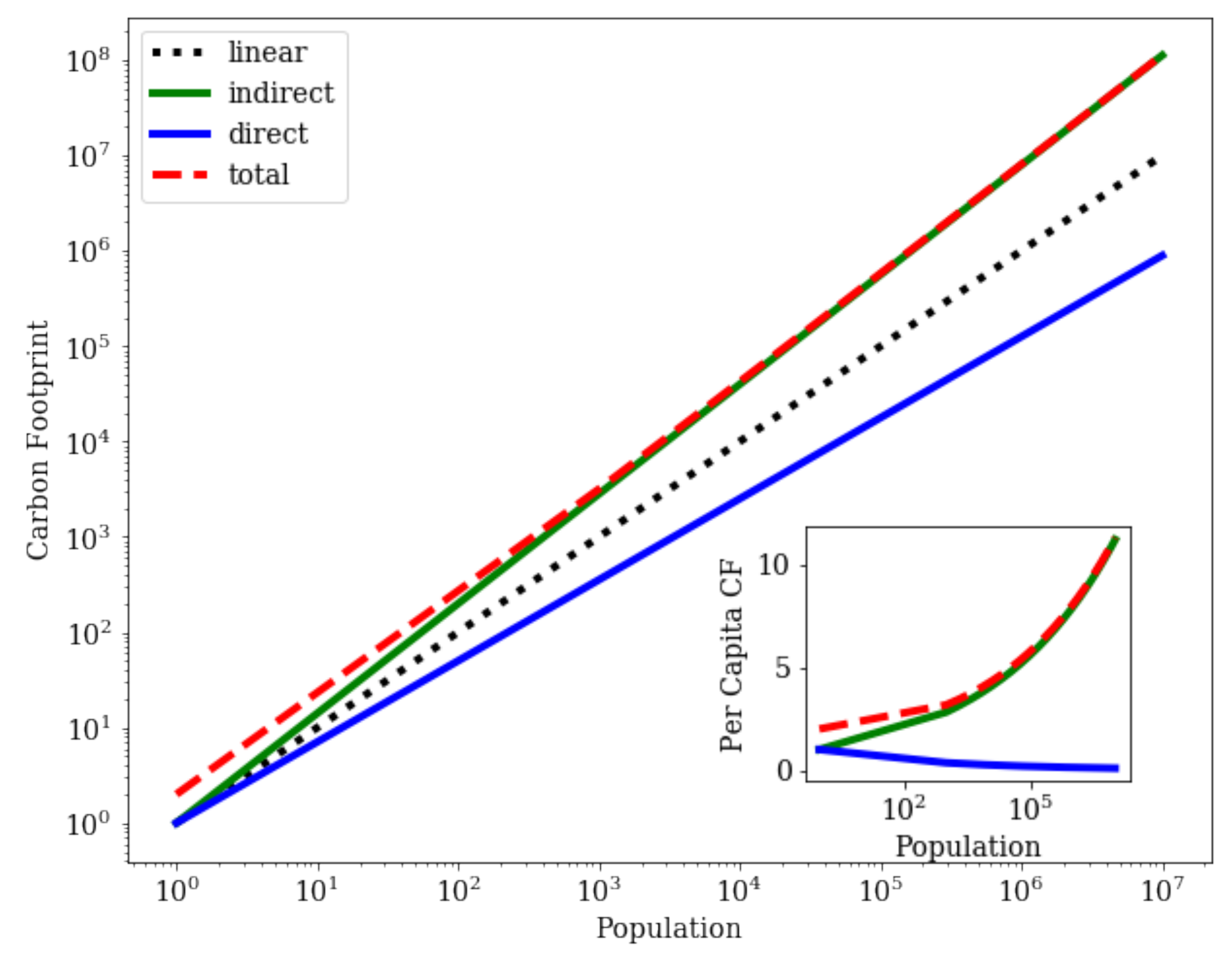
4. A Toy Model of Urban Carbon Footprint Based on Scaling Laws

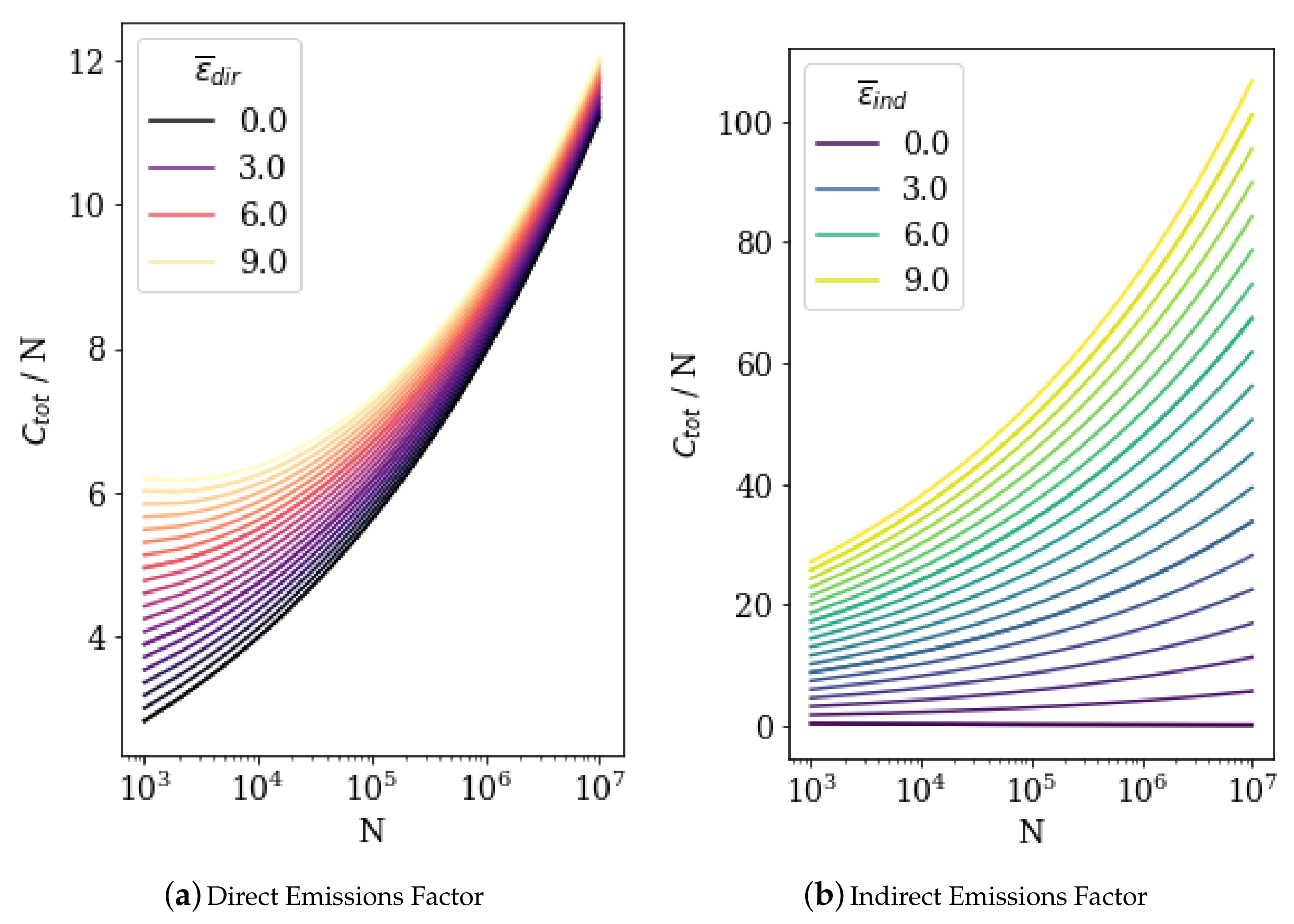
4.1. Environmental Rebound Effect of City Size

As a first approach, we propose a naive scaling model assuming scaling properties from literature. We will assume that the total carbon footprint of a city (in tons of CO${}_2$) represented by $C_{tot}$ can be divided into (i) direct emissions, $C_{dir}$; and (ii) indirect emissions, $C_{ind}$. That is,

$$C_{tot}=C_{dir}+C_{ind}.$$

(2)

We define $C_{dir}$ as the sum of territorial emissions (TE) and community-wide infrastructure-based carbon footprint (CIF) which rests within the city boundaries. That is, it accounts for emissions occurring within the city boundary (e.g., gasoline consumption), emissions embedded in grid-supplied electricity and emissions embedded in infrastructure (roads, water pipes, buildings), but not for emissions occurring in factories or other production processes. Differently, $C_{ind}$ is defined here as all other emissions taking place outside the city boundaries as a consequence of activities occurring within the city boundaries (e.g., emissions embedded in goods and services).

Emissions from a given activity can be estimated by multiplying the activity data, which can be computed in monetary terms, by the activity emission factor $\overline{ϵ}$ [26]. In our toy model, we assume that $\overline{ϵ}$ can be described as the mean emission factor for the type of activity (direct or indirect). If every activity (e.g., buying a t-shirt, or 1 kg of cement, or 1 kWh of electricity) holds one associated emission factor, one can draw a probability distribution of emission factors by money expenditure for a city and estimate its average value (that is, $\overline{ϵ}$).

In our model, $C_{dir}$ describes emissions related to spatially-embedded infrastructures, such as upstream emissions from resources for the building stocks, emissions embedded in electricity for housing and in gasoline for transportation. Let’s consider that $C_{dir}$ of a city is directly dependent on its total expenditure in infrastructure. This way, one can write that $C_{dir}={\overline{ϵ}}_{dir}·Y_{inf}$, where $Y_{inf}$ is the city’s total expenditure related to spatially-embedded infrastructure (in purchasing power parities (PPP) measured in National currency units/US dollar), and ${\overline{ϵ}}_{dir}$ is the mean direct emission factor.

On the other hand, $C_{ind}$ describes emissions related to the consumption of goods and services by the population and it is driven by the population’s income. In our model, we will assume that $C_{ind}$ is directly dependent on the city’s total income (in PPP USD), which will be represented by $Y_{inc}$. Then, one can assert that $C_{ind}={\overline{ϵ}}_{ind}·Y_{inc}$, where ${\overline{ϵ}}_{ind}$ is the mean indirect emission factor. With a better definition of $C_{dir}$ and $C_{ind}$, Equation (2) can be re-written as

$$C_{tot}={\overline{ϵ}}_{dir}·Y_{inf}+{\overline{ϵ}}_{ind}·Y_{inc}.$$

(3)

Here we bring in the stylized facts observed in the urban scaling hypothesis. We assume that the city’s total expenditure related to spatially-embedded infrastructure scales as any infrastructure-related variable, following the power-law

$$Y_{inf}\approx Y_{inf}^0{N}^{{\beta }_{inf}},$$

(4)

where $Y_{inf}^0$ is the intercept, and ${\beta }_{inf}<1$ (sublinear regime).

Similarly, we assume, based on the urban scaling hypothesis, that the city’s disposable income follows the expected scaling behavior of socioeconomic variables, known to scale in a super-linear manner with the city’s population N by the power-law

$$Y_{inc}\approx Y_{inc}^0{N}^{{\beta }_{inc}},$$

(5)

where $Y_{inc}^0$ is the intercept, and ${\beta }_{inc}>1$ is the scaling exponent. This is an approximation: disposable income is just a fraction of the city’s GDP and although other variables related to expenditure, income and wages have been observed to scale in a superlinear manner with population [15,16,69,70,71], to the best of our knowledge no study has explicitly estimated the scaling of disposable income.

If we assume that both scaling exponents are correlated [6,16,17], that is if ${\beta }_{inc}=1+\delta$ and ${\beta }_{inf}=1-\delta$, then Equation (3) can be re-written as

$$C_{tot}={\overline{ϵ}}_{dir}·Y_{inf}^0{N}^{1-\delta }+{\overline{ϵ}}_{ind}·Y_{inc}^0{N}^{1+\delta }.$$

(6)

By solving Equation (6) computationally, we got the results presented in Figure 4. In order to understand the naive scaling of CF, we assumed ${\overline{ϵ}}_{dir}={\overline{ϵ}}_{ind}=Y_{inf}^0=Y_{inc}^0=1$ and $\delta =0.15$. Later on, we will further explore the effect of each variable.

We can observe that, as the population N increases, the indirect carbon footprint $C_{ind}\sim N^{1+\delta }$ (green line) becomes more and more important to the total carbon emission $C_{tot}$ (red dashed line). That is, when N is sufficiently large, $C_{tot}\sim N^{1+\delta }$. This means a super-linear power-law relation between the total carbon emission and the population size, and it is independent of the values of the emission factors and the intercepts. The naive scaling model contradicts Brand’s Law or the belief that bigger cities are greener. The model indicates a backfire rebound effect from city size/density: once emissions embedded in goods and services (scope 3) are included on top of the spatial-related emissions, bigger cities are expected to have higher emissions per capita than smaller ones (Figure 4 bottom-right). We will see below that it is possible to find certain configurations of parameters that maintain the scaling sublinear for a limited but still feasible population range (for example 1000 ≤ N ≤ 10,000,000).

The Naive model assumes the same emission factor for both direct and indirect emissions (${\overline{ϵ}}_{dir}$ = ${\overline{ϵ}}_{ind})$ and the same intercept for both the income and infrastructure ($Y_{inf}^0=Y_{inc}^0$). This is unlikely to be realistic, and we will explore next the effect of varying emission factors and intercepts on the scaling of emissions (Figure 5).

As a matter of fact, Equation (6) can be re-written as follows:

$$\begin{array}{ccc}\hfill C_{tot}& =& {\overline{ϵ}}_{dir}·Y_{inf}^0{N}^{1-\delta }+{\overline{ϵ}}_{ind}·Y_{inc}^0{N}^{1+\delta }\hfill \\ & =& N[{\overline{ϵ}}_{dir}·Y_{inf}^0{N}^{-\delta }+{\overline{ϵ}}_{ind}·Y_{inc}^0{N}^{+\delta }]\hfill \\ & =& N{\overline{ϵ}}_{dir}·Y_{inf}^0\left[N^{-\delta }+\frac{{\overline{ϵ}}_{ind}·Y_{inc}^0}{{\overline{ϵ}}_{dir}·Y_{inf}^0}{N}^{+\delta }\right],\hfill \end{array}$$

and therefore

$$\begin{array}{ccc}\hfill C_{tot}& \propto & N\left[N^{-\delta }+\left(\frac{{\overline{ϵ}}_{ind}}{{\overline{ϵ}}_{dir}}\right)\left(\frac{Y_{inc}^0}{Y_{inf}^0}\right)N^{\delta }\right].\hfill \end{array}$$

Which can be re-written in per capita terms

$$\frac{C_{tot}}{N}\propto N^{-\delta }+\left(\frac{{\overline{ϵ}}_{ind}}{{\overline{ϵ}}_{dir}}\right)\left(\frac{Y_{inc}^0}{Y_{inf}^0}\right)N^{\delta }.$$

(7)

These results show how the ratios between the emission factors (${\overline{ϵ}}_{ind}/{\overline{ϵ}}_{dir}$) and the intercepts ($Y_{inc}^0/Y_{inf}^0$) influence the dynamics of per capita CF. When one of the factors assume very small values then $N^{-\delta }$ governs the equation, producing a sublinear scaling. When the indirect emissions factor is much smaller than the direct emissions factor (${\overline{ϵ}}_{ind}\ll {\overline{ϵ}}_{dir}$) or the income intercept is much smaller than the infrastructure spend intercept ($Y_{inc}^0\ll Y_{inf}^0$), then the term $N^{\delta }$ governs the equation, producing a superlinear scaling regime. In this case, bigger cities become greener than smaller ones. Figure 6 presents per capita emissions difference between the smallest (N = 1000) and biggest (N = 10,000,000) cities in the simulation as a function of ${\overline{ϵ}}_{ind}/{\overline{ϵ}}_{dir}$. It is possible to observe that for ${\overline{ϵ}}_{ind}/{\overline{ϵ}}_{dir}$ < 0.03 bigger cities emit less carbon per capita than smaller ones, while for ${\overline{ϵ}}_{ind}/{\overline{ϵ}}_{dir}$ > 0.03 bigger cities emit more carbon per capita than smaller ones, regardless of the absolute parameter values. The same behavior is true for $Y_{inf}^0/Y_{inc}^0$.

While the direct emission factor (${\overline{ϵ}}_{dir}$) has only a small effect on the curve describing the relation between the population N of a city and the per capita carbon footprint $C_{tot}$, the indirect emission factor (${\overline{ϵ}}_{ind}$) can completely decouple emissions from the city size. For very small indirect emission factors, bigger cities do not show larger emissions. Different values of ${\overline{ϵ}}_{ind}$ diverge the trajectory of per capita CF, while different values of ${\overline{ϵ}}_{dir}$ produce very similar curves of per capita CF, as presented in Figure (Figure 5). This happens because, for very small indirect emission factors, the superlinear scaling of indirect CF can be neglected. However, this only happens for very small values of ${\overline{ϵ}}_{ind}$, which might be an unrealistic scenario only achievable by very efficient production processes or by an impact-less consumption pattern by most of the city’s population. The same analysis holds true for the intercepts, with $Y_{inc}^0$ producing a similar behavior as ${\overline{ϵ}}_{ind}$.

4.2. Decoupling Economic Growth from Environmental Impacts

There is a hidden assumption in the previous model: we have considered that the emission factors (direct and indirect) were independent from income and population size. This means that the impact factors are constant across the population range of simulated cities. In other words, the naive version assumes that: (i) for direct emissions: the materials and production processes adopted in infrastructure construction and operation are the same across cities with different population and wealth levels; and (ii) for indirect emissions: citizens with different income levels and from cities of all sizes consume the same type of goods and services, following the same consumption distribution. This is unlikely to be true, given that: (i) bigger cities are potentially able to implement more diverse infrastructure technologies than smaller ones, with different environmental impacts [73]; and (ii) within the same urban system, inhabitants of bigger cities tend to be wealthier than those from smaller cities, and wealthier people do have different consumption patterns and associated environmental impacts than poor ones [85]. In addition, residents of large cities have more opportunities for consumption. It is important to test under which conditions bigger cities are greener than smaller ones considering all these effects.

What we will be testing is whether decoupling can offset the rebound effect of city size. The decoupling of economic growth from environmental impacts is defined as the reduction of environmental impacts per unit of economic output, meaning that the economy can grow with a less than proportional increase in its associated environmental impacts (relative decoupling) or even without increasing at all its associated environmental impacts (absolute decoupling) [86]. Conversely, coupling comes into being when an economy experiences an increase in environmental impacts per unit of economic output. Consumption-based decoupling is relatively rare to observe, but it can happen in countries across all levels of economic development. A recent study [87] found that between 2000 and 2014, out of 124 countries, 27 have experienced absolute decoupling, while 17 faced relative decoupling and 80 have endured a coupling between carbon footprint and economic growth. While absolute decoupling for the whole economy might be impossible to sustain indefinitely [88], an urban system might achieve Brand’s Law through the relative decoupling along with spatial efficiencies of its cities.

To reach a more realistic model and test the role of decoupling in urban sustainability, we considered that the the emission factor will be a function of wealth, that is: ${\overline{ϵ}}_{dir}\to {\overline{ϵ}}_{dir}\left(Y_{inf}\right)$, and ${\overline{ϵ}}_{ind}\to {\overline{ϵ}}_{ind}\left(Y_{inc}\right)$. With this consideration, Equation (3) becomes:

$$C_{tot}={\overline{ϵ}}_{dir}\left(Y_{inf}\right)·Y_{inf}+{\overline{ϵ}}_{ind}\left(Y_{inc}\right)·Y_{inc}.$$

(8)

We can infer the expected relation between income and emissions factor ($\overline{ϵ}$) from the better-studied relation between wealth (Y) and carbon emissions ($C_{tot}$), known to follow a power law with an exponent $\gamma$ [85,89,90]. That is

$$C=C^0{Y}^{\gamma },$$

(9)

which allows us to write $\overline{ϵ}\left(Y\right)\propto C/Y=C^0{Y}^{\gamma -1}$, which in turn yields

$$\overline{ϵ}\left(Y\right)\propto Y^{\gamma -1}.$$

(10)

Given that wealth also scales as a power law with the population ($Y\sim N^{1+\delta }$), the result above can be re-written as

$$\overline{ϵ}\left(Y\right)\propto N^{(1+\delta ).(\gamma -1)}.$$

(11)

Here, we propose that direct and indirect emissions would assume different scaling exponents, which we will call ${\gamma }_{inf}$ and ${\gamma }_{inc}$, respectively. This is related to the fact that the carbon intensity of infrastructure and consumption follows different decoupling behaviors. It allows us to write (from Equation (11))

$${\overline{ϵ}}_{dir}\left(Y_{inf}\right)=C_{dir}^0{N}^{(1+\delta ).({\gamma }_{inf}-1)},$$

(12)

and

$${\overline{ϵ}}_{ind}\left(Y_{inc}\right)=C_{ind}^0{N}^{(1+\delta ).({\gamma }_{inc}-1)}.$$

(13)

While the first is mainly driven by technology and investment capacity, the second is also driven by social-economic norms. Inserting the relations (12) and (13) into Equation (8), we get

$$C_{tot}=A·N^{{\gamma }_{inf}(1-\delta )}+B·N^{{\gamma }_{inc}(1+\delta )},$$

(14)

which is a more general way to write the total carbon emission. Here, we introduced the constants $A\equiv C_{dir}^0·Y_{inf}^0$ and $B\equiv C_{ind}^0·Y_{inc}^0$.

Empirical values for $\gamma$ vary significantly from country to country. Authors tend to agree that the most common values in country-wide regressions are smaller than 1 [85,89,90]. That said, a recent consumption-based study found values evenly distributed between 0.5 and 1.5 for regression within countries [82]. It is worth noticing that, once again, empirical evidence here is mainly based on production accounting methods at the national level. Our strategy to deal with such empirical faults will be to test the “phase-space” of the scaling exponent, instead of proposing one value. Figure 7 presents the scaling between per capita $C_{tot}$ and city population in our model, considering different values for both ${\gamma }_{inf}$ and ${\gamma }_{inc}$.

Figure 7 describes the elasticity between income and indirect emissions. We can observe that ${\gamma }_{inc}$ is the key variable in the model, defining the scaling regime between population and carbon footprint. Very different results can be obtained from a small value of ${\gamma }_{inc}$: sufficiently large values produce superlinear scaling of per capita $C_{tot}$ with population, while sufficiently small values produce sublinear scaling. Notice that ${\gamma }_{inf}={\gamma }_{inc}=1$ retrieve the naive model, with $\overline{ϵ}$ assuming a constant relation with income and population. This relation could explain the diversity of relations found between city size and consumption-based emissions for different countries. On top of that, the fact that countries from the global south tend to present higher values for ${\gamma }_{inc}$ [87] can potentially explain the predominance of the conclusion “bigger is not greener” in those countries, while smaller values for ${\gamma }_{inc}$ in the global south could lead to “bigger is greener”, as empirically observed [81].

In order to obtain the most of the theoretical analysis of the model, let us consider hereafter, by convenience only, that $\gamma \equiv {\gamma }_{inf}={\gamma }_{inc}$. With this consideration it will be possible to find the critical value of $\gamma$, say ${\gamma }^{*}$, which shifts the scaling regime of $C_{tot}$ from superlinear to sublinear. In order to do that, let us rewrite Equation (14) as

$$C_{tot}=N^{\gamma }[A·N^{-\gamma ·\delta }+B·N^{\gamma ·\delta }].$$

(15)

Letting $N\stackrel{}{\to }\infty$ and being $B·N^{\gamma ·\delta }$ sufficiently small, we get

$$C_{tot}\approx N^{\gamma (1+\delta )}.$$

(16)

Therefore, the limit between superlinear and sublinear scaling is given by ${\gamma }^{*}(1+\delta )=1$ and consequently

$${\gamma }^{*}=\frac{1}{1+\delta }.$$

(17)

Figure 8 illustrates the phase-space diagram of expected scaling regime of total carbon footprint ($C_{tot}$) given different values of $\gamma$. For $\gamma >\frac{1}{(1+\delta )}$, total emissions scale in a superlinear manner with the population; that is, for a sufficiently large $\gamma$, larger cities are more polluting, breaking Brand’s Law. While for $\gamma <\frac{1}{(1+\delta )}$ a sub-linear regime is observed; that is, Brand’s Law only works if the scaling exponent $\gamma$ is smaller than the threshold value. For $\gamma =\frac{1}{(1+\delta )}$, a linear regime is retrieved, with total emissions growing proportionally to the population (${\gamma }^{*}$ represented by the dashed line in Figure 8).

5. Discussion

This paper looks into the question whether bigger cities are greener or not. In doing so, we proposed a mean-field model to derive emission estimations out of well-established urban metrics (e.g., city size, density and infrastructure). Our results suggest that Brand’s Law’s premise—bigger cities are necessarily greener—only holds true when we consider territorial-based emissions alone. In turn, when we take consumption-based emissions into account, Brand’s Law does fall apart in most cases. One reason for this, is that bigger cities have greater purchasing power, which implies a higher consumption of goods. Indeed, despite ongoing efforts to reduce carbon footprint in economic production, greater consumption leads to higher associated GHG emissions [91,92,93]. Thus, benefits of economy of scale are overruled by increasing consumption.

As previously discussed, these mismatches in results arise as most methodologies fail in the attempt to estimate actual emissions due to (i) the lack of data available on consumption-based emissions, and (ii) the lack of a consensus methodology to be used for this purpose [94,95]. As shown above, Brand’s law’s premise is usually assessed on estimated amounts of GHG emissions which do not necessarily reflect the real figures [92]. Therefore, indirect consumption-based emissions are either not considered or underestimated. These weaknesses apply even more for calculating the final carbon footprint since the current methods involve inaccurate measures of both direct and indirect emissions.

The model introduced in this article shows that the assumptions of Brand’s Law impose limitations to more complete and accurate descriptions of how city size relates to carbon emissions. The toy model proposed also provides a new way of studying the link between city size and GHG emissions that allows for identifying the phases of transition between a superlinear and sublinear regime, indicating potential avenues for policy making in urban contexts.

Our analysis also has some caveats. We do not differentiate between prices or consumption patterns in cities with different sizes or cultures, which of course is not the case in real-world situations. Future research should also pay attention to consumption disparities among different social strata, and to adequate simulations of the effects of population increases on income and, consequently, on consumption [85,96].

Despite these limitations, the model proposed also shows that the decoupling of population from emissions is possible and dependent on the decoupling level between income and environmental impacts. In order to achieve this in reality, a shift in consumption patterns is of utmost importance [91,93]. Such shift should imply that every new monetary unit added to the GDP, or any other income variable for that effect, does not result in proportional or more than proportional increases in GHG emissions. In other words, in addition to ecological efficiency, society must strive for finding limits to how income patterns turn into purchase power and consumption.

These issues are also embedded in normative challenges. It is hard to create policies aiming at reducing consumption-based emissions because production is frequently out of reach, falling under different economies and legislation. Global efforts would be necessary to coordinate strategies and take cities as the primary loci of production and consumption in order to change such patterns [85,93] and properly reduce GHG emissions.

Finally, we acknowledge that the caveats in our analyses, mainly regarding carbon footprint data, result in inaccurate estimations of direct and indirect emissions. This specific issue leads to difficulties in empirically testing the model introduced in this paper, or any other model intended to analyze carbon emissions of any given social system-or Brand’s Law itself, for that matter. Indeed more research is needed to better estimate indirect emissions in particular.

6. Conclusions

Our model brings some assumptions due to the lack of empirical support: (i) the scaling exponent of disposable income is proportional to that of total GDP in a system of cities; (ii) prices along with (iii) consumption patterns are the same in cities across the population interval. Furthermore, the model could be fine-tuned by including (a) a scaling exponent explicitly related to disposable income of cities; (b) a purchasing power parity price model; and (c) the consideration of different consumption patterns. Those changes, however, should not dismiss the general findings of the model. Although the exact value of the threshold scaling exponent (${\gamma }^{*}$) from which bigger cities fail to be “greener” would probably change, the fact that there is a limit-value should not change.

From a broader perspective, the model proposed in this work is a mean field toy model, not accounting for local specificities but general standards, which limits the practical application of its results. A statistical mechanics approach should be developed in order to account for local specificities. Due to the lack of available empirical data, the model cannot be validated at this stage. Given the importance concerning goods consumption in bigger cities, a methodological possibility to overcome this is by using credit card data associated with multi-regional input-output emission models (MRIO), generating emissions estimations directly from consumption. Applying the same method for a range of city sizes could lead to more reliable comparisons between indirect emission estimations.

The present work has been based on up-to-date knowledge on scaling properties, urban systems and GHG emissions. Limits to accuracy in results can be overcome once the interdisciplinary fields involved reach a deeper understanding of the internal workings of cities, more robust statistical exponents in scaling and more accurate methods for GHG estimations. We expect this model to contribute to the analysis of relations of city size to environmental impacts, the coupling of economic growth and emissions and the design of policies able to decouple them in order to achieve truly sustainable cities. Finally, this work hopes to contribute to a broader assessment of the causes of emissions and the possibility of a paradigm shift regarding the assumption of efficiency in the relationship of city size and emissions, adding consumption behavior as a critical variable, and going beyond Brand’s Law.

References

1. Seto, K.C.; Solecki, W.D.; Griffith, C.A. The Routledge Handbook of Urbanization and Global Environmental Change; Routledge: London, UK, 2015. [Google Scholar]
2. Glaeser, E.L.; Kahn, M.E. The greenness of cities: Carbon dioxide emissions and urban development. J. Urban Econ. 2010, 67, 404–418. [Google Scholar] [CrossRef] [Green Version]
3. Rybski, D.; Reusser, D.E.; Winz, A.L.; Fichtner, C.; Sterzel, T.; Kropp, J.P. Cities as nuclei of sustainability? Environ. Plan. B Urban Anal. City Sci. 2017, 44, 425–440. [Google Scholar] [CrossRef] [Green Version]
4. Pachauri, R.K.; Allen, M.R.; Barros, V.R.; Broome, J.; Cramer, W.; Christ, R.; Church, J.A.; Clarke, L.; Dahe, Q.; Dasgupta, P.; et al. Climate Change 2014: Synthesis Report. Contribution of Working Groups I, II and III to the Fifth Assessment Report of the Intergovernmental Panel on Climate Change; IPCC: Geneva, Switzerland, 2014. [Google Scholar]
5. Angel, S. Planet of Cities; Lincoln Institute of Land Policy: Cambridge, MA, USA, 2012. [Google Scholar]
6. West, G.B. Scale: The Universal Laws of Growth, Innovation, Sustainability, and the Pace of Life in Organisms, Cities, Economies, and Companies; Penguin Press: New York, NY, USA, 2017. [Google Scholar]
7. Barthelemy, M. The Structure and Dynamics of Cities; Cambridge University Press: Cambridge, UK, 2016. [Google Scholar]
8. Batty, M. The New Science of Cities; MIT Press: Cambridge, MA, USA, 2013. [Google Scholar]
9. Norman, J.; MacLean, H.L.; Kennedy, C.A. Comparing high and low residential density: Life-cycle analysis of energy use and greenhouse gas emissions. J. Urban Plan. Dev. 2006, 132, 10–21. [Google Scholar] [CrossRef]
10. Newman, P.W.; Kenworthy, J.R. Gasoline consumption and cities: A comparison of us cities with a global survey. JAPA 1989, 55, 24–37. [Google Scholar] [CrossRef]
11. Behsh, B. Building form as an option for enhancing the indoor thermal conditions. In Proceedings of the Building Physics 2002—6th Nordic Symposium, Trondheim, Norway, 17–19 June 2002. [Google Scholar]
12. Bettencourt, L.M.; West, G.B. Bigger cities do more with less. Sci. Am. 2011, 305, 52–53. [Google Scholar] [CrossRef]
13. Geddes, P. Civics: As Applied Sociology; Leicester University Press: Leicester, UK, 1979. [Google Scholar]
14. Ahrend, R.; Farchy, E.; Kaplanis, I.; Lembcke, A.C. What Makes Cities More Productive? Evidence on the Role of Urban Governance from Five OECD Countries. OECD Reg. Dev. Work. Pap. 2014, 1–33. [Google Scholar] [CrossRef]
15. Bettencourt, L.M.; Lobo, J.; Helbing, D.; Kühnert, C.; West, G.B. Growth, innovation, scaling, and the pace of life in cities. Proc. Natl. Acad. Sci. USA 2007, 104, 7301–7306. [Google Scholar] [CrossRef] [Green Version]
16. Bettencourt, L.M. The origins of scaling in cities. Science 2013, 340, 1438–1441. [Google Scholar] [CrossRef] [Green Version]
17. Ribeiro, F.L.; Meirelles, J.; Ferreira, F.F.; Neto, C.R. A model of urban scaling laws based on distance-dependent interactions. R. Soc. Open Sci. 2017, 4, 160926. [Google Scholar] [CrossRef] [Green Version]
18. Jacobs, J. The Death and Life of Great American Cities; Random House: New York, NY, USA, 1961. [Google Scholar]
19. Soja, E. Writing the city spatially. City 2003, 7, 269–280. [Google Scholar] [CrossRef]
20. Jacobs, J. The Economy of Cities; Random House: New York, NY, USA, 1969. [Google Scholar]
21. Seto, K.C.; Dhakal, S.; Bigio, A.; Blanco, H.; Delgado, G.C.; Dewar, D.; Huang, L.; Inaba, A.; Kansal, A.; Lwasa, S.; et al. Human settlements, infrastructure and spatial planning. In Climate Change 2014: Mitigation of Climate Change. Contribution of Working Group III to the Fifth Assessment Report of the Intergovernmental Panel on Climate Change; Cambridge University Press: Cambridge, UK, 2014. [Google Scholar]
22. C40 Cities Climate Leadership Group. Consumption-Based GHG Emissions of C40 Cities. Available online: http://www.c40.org/researches/consumption-based-emissions (accessed on 2 July 2019).
23. Steininger, K.; Lininger, C.; Droege, S.; Roser, D.; Tomlinson, L.; Meyer, L. Justice and cost effectiveness of consumption-based versus production-based approaches in the case of unilateral climate policies. Glob. Environ. Chang. 2014, 24, 75–87. [Google Scholar] [CrossRef]
24. Chen, G.; Shan, Y.; Hu, Y.; Tong, K.; Wiedmann, T.; Ramaswami, A.; Guan, D.; Shi, L.; Wang, Y. A review on city-level carbon accounting. Environ. Sci. Technol. 2019, 53, 5545–5558. [Google Scholar] [CrossRef]
25. Janet, R.; Laurent, C.; Simon, S.; Kjell, O.; Brian, D.; Matt, S.; Mike, B.; Pierre, B.; Environment, C.; Rob, F.; et al. The Greenhouse Gas Protocol: A Corporate Accounting and Reporting Standard; WBCSD/WRI 2004; World Resources Institute: Washington, DC, USA, 2004. [Google Scholar] [CrossRef]
26. Fong, W.K.; Sotos, M.; Doust, M.M.; Schultz, S.; Marques, A.; Deng-Beck, C. Global Protocol for Community-Scale Greenhouse Gas Emission Inventories (gpc); World Resources Institute: New York, NY, USA, 2015. [Google Scholar]
27. Mi, Z.; Zhang, Y.; Guan, D.; Shan, Y.; Liu, Z.; Cong, R.; Yuan, X.C.; Wei, Y.M. Consumption-based emission accounting for chinese cities. Ecol. Indic 2014, 47, 26–31. [Google Scholar] [CrossRef] [Green Version]
28. Dhakal, S.; Hidefumi, I. Urban Energy Use and Greenhouse Gas Emissions in Asian Mega-Cities: Policies for a Sustainable Future; Urban Environmental Management Project; Institute for Global Environmental: Hayama, Japan, 2004. [Google Scholar]
29. Minx, J.; Baiocchi, G.; Wiedmann, T.; Barrett, J.; Creutzig, F.; Feng, K.; Förster, M.; Pichler, P.P.; Weisz, H.; Hubacek, K. Carbon footprints of cities and other human settlements in the uk. Environ. Res. Lett. 2013, 8, 35039. [Google Scholar] [CrossRef]
30. Gill, B.; Moeller, S. Ghg emissions and the rural-urban divide. a carbon footprint analysis based on the german official income and expenditure survey. Ecol. Econ. 2018, 145, 160–169. [Google Scholar] [CrossRef]
31. Heinonen, J.; Kyrö, R.; Junnila, S. Dense downtown living more carbon intense due to higher consumption: A case study of helsinki. Environ. Res. Lett. 2011, 6, 034034. [Google Scholar] [CrossRef]
32. Jones, C.; Kammen, D.M. Spatial distribution of us household carbon footprints reveals suburbanization undermines greenhouse gas benefits of urban population density. Environ. Sci. Technol. 2014, 48, 895–902. [Google Scholar] [CrossRef]
33. Sudmant, A.; Gouldson, A.; Millward-Hopkins, J.; Scott, K.; Barrett, J. Producer cities and consumer cities: Using production-and consumption-based carbon accounts to guide climate action in china, the uk, and the us. J. Clean. Prod. 2018, 176, 654–662. [Google Scholar] [CrossRef]
34. Netto, V.M.; Vargas, J.C.B.; Saboya, R.T. A revolução dos dados e a nova ciência das cidades (Editorial). RMU 2020, 8, e00173. [Google Scholar] [CrossRef]
35. Ribeiro, F.L. Física das Cidades. RMU 2020, 8, e00159. [Google Scholar] [CrossRef]
36. Bettencourt, L.; West, G. A unified theory of urban living. Nature 2010, 467, 912. [Google Scholar] [CrossRef]
37. Netto, V.M.; Meirelles, J.; Ribeiro, F.L. Social Interaction and the City: The Effect of Space on the Reduction of Entropy. Complexity 2017, 2017. [Google Scholar] [CrossRef] [Green Version]
38. Bettencourt, L.M.; Lobo, J. Urban scaling in europe. J. R. Soc. Interface 2016, 13, 20160005. [Google Scholar] [CrossRef]
39. Ortman, S.G.; Cabaniss, A.H.; Sturm, J.O.; Bettencourt, L.M. The pre-history of urban scaling. PLoS ONE 2014, 9, e87902. [Google Scholar] [CrossRef]
40. Gomez-Lievano, A.; Youn, H.; Bettencourt, L.M.A. The statistics of urban scaling and their connection to zipf’s law. PLoS ONE 2012, 7, e40393. [Google Scholar] [CrossRef]
41. Gomez-Lievano, A.; Youn, H.; Bettencourt, L.M. Scaling in transportation networks. PLoS ONE 2014, 9, e102007. [Google Scholar]
42. Adhikari, P.; de Beurs, K.M. Growth in urban extent and allometric analysis of west african cities. J. Land Use Sci. 2017, 12, 105–124. [Google Scholar] [CrossRef]
43. Meirelles, J.; Neto, C.R.; Ferreira, F.F.; Ribeiro, F.L.; Binder, C.R. Evolution of urban scaling: Evidence from brazil. PLoS ONE 2018, 13, e0204574. [Google Scholar] [CrossRef] [PubMed] [Green Version]
44. Krugman, P. Increasing returns and economic geography. J. Political Econ. 1991, 99, 483–499. [Google Scholar] [CrossRef]
45. Schläpfer, M.; Bettencourt, L.M.A.; Grauwin, S.; Raschke, M.; Claxton, R.; Smoreda, Z.; West, G.B.; Ratti, C. The scaling of human interactions with city size. J. R. Soc. Interface 2014, 11, 20130789. [Google Scholar] [CrossRef] [PubMed]
46. Ribeiro, F.L.; Meirelles, J.; Netto, V.M.; Neto, C.R.; Baronchelli, A. On the relation between Transversal and Longitudinal Scaling in Cities. PLoS ONE 2020, 15, e0233003. [Google Scholar]
47. Youn, H.; Bettencourt, L.M.; Lobo, J.; Strumsky, D.; Samaniego, H.; West, G.B. Scaling and universality in urban economic diversification. Interface 2016, 13, 20150937. [Google Scholar] [CrossRef] [Green Version]
48. Depersin, J.; Barthelemy, M. From global scaling to the dynamics of individual cities. Proc. Natl. Acad. Sci. USA 2017, 115, 1–6. [Google Scholar] [CrossRef] [Green Version]
49. Molinero, C.; Thurner, S. How the geometry of cities explains urban scaling laws and determines their exponents. arXiv 2019, arXiv:1908.07470. [Google Scholar]
50. Arcaute, E.; Hatna, E.; Ferguson, P.; Youn, H.; Johansson, A.; Batty, M. Constructing cities, deconstructing scaling laws. J. R. Soc. Interface 2015, 12, 20140745. [Google Scholar] [CrossRef]
51. Louf, R.; Barthelemy, M. Scaling: Lost in the smog. Environ. Plan. B Plan. Des. 2014, 41, 767–769. [Google Scholar] [CrossRef] [Green Version]
52. Leitao, J.C.; Miotto, J.M.; Gerlach, M.; Altmann, E.G. Is this scaling nonlinear? R. Soc. Open Sci. 2016, 3, 150649. [Google Scholar] [CrossRef] [Green Version]
53. Strano, E.; Sood, V. Rich and poor cities in europe. an urban scaling approach to mapping the european economic transition. PLoS ONE 2016, 11, e0159465. [Google Scholar] [CrossRef]
54. Muller, N.Z.; Jha, A. Does environmental policy affect scaling laws between population and pollution? evidence from american metropolitan areas. PLoS ONE 2017, 12, e0181407. [Google Scholar] [CrossRef] [Green Version]
55. Batty, M.; Ferguson, P. Defining city size. Environ. Plan. B Plan. Des. 2011, 38, 753–756. [Google Scholar] [CrossRef]
56. Cesaretti, R.; Lobo, J.; Bettencourt, L.M.; Ortman, S.G.; Smith, M.E. Population-area relationship for medieval european cities. PLoS ONE 2016, 11, e0162678. [Google Scholar] [CrossRef] [Green Version]
57. Stewart, J.Q.; Warntz, W. Physics of population distribution. J. Reg. Sci. 1958, 1, 99–121. [Google Scholar] [CrossRef]
58. Nordbeck, S. Urban allometric growth. Geogr. Ann. Ser. B 1971, 53, 54–67. [Google Scholar] [CrossRef]
59. Paulsen, K. Yet even more evidence on the spatial size of cities: Urban spatial expansion in the us, 1980–2000. Reg. Sci. Urban Econ. 2012, 42, 561–568. [Google Scholar] [CrossRef]
60. Cottineau, C.; Hatna, E.; Arcaute, E.; Batty, M. Diverse cities or the systematic paradox of urban scaling laws. Comput. Environ. Urban 2017, 63, 80–94. [Google Scholar] [CrossRef] [Green Version]
61. Cleveland, T.; Dec, P.; Rainham, D. Shorter Roads go a Long Way: The relationship between density and road length per resident within and between cities. Can. Plan. Policy 2020, 2020, 71–89. [Google Scholar]
62. Ribeiro, H.V.; Rybski, D.; Kropp, J.P. Effects of changing population or density on urban carbon dioxide emissions. Nat. Commun. 2019, 10, 3204. [Google Scholar] [CrossRef] [PubMed] [Green Version]
63. Um, J.; Son, S.W.; Lee, S.I.; Jeong, H.; Kim, B.J. Scaling laws between population and facility densities. Proc. Natl. Acad. Sci. USA 2009, 106, 14236–14240. [Google Scholar] [CrossRef] [Green Version]
64. Netto, V.M.; Ribeiro, F.L.; Silva de Carvalho, C.L.; Cabral, V.; Neto, C. As Cidades na Pandemia: O Papel do Tamanho e da Densidade Urbana. Available online: https://caosplanejado.com/as-cidades-na-pandemia-o-papel-do-tamanho-e-da-densidade-urbana/ (accessed on 2 July 2020).
65. Fragkias, M. Urbanization, economic growth and sustainability. In The Routledge Handbook of Urbanization and Global Environmental Change; Routledge: London, UK, 2015; pp. 33–50. [Google Scholar]
66. Quigley, J.M. Urban diversity and economic growth. JEP 1998, 12, 127–138. [Google Scholar] [CrossRef] [Green Version]
67. Fujita, M. Urban Economic Theory: Land Use and City Size; Cambridge University Press: Cambridge, UK, 1989. [Google Scholar]
68. Van Raan, A.F.; Van Der Meulen, G.; Goedhart, W. Urban scaling of cities in the netherlands. PLoS ONE 2016, 11, e0146775. [Google Scholar] [CrossRef] [Green Version]
69. Alves, L.G.; Ribeiro, H.V.; Lenzi, E.K.; Mendes, R.S. Distance to the scaling law: A useful approach for unveiling relationships between crime and urban metrics. PLoS ONE 2013, 8, e69580. [Google Scholar] [CrossRef]
70. Ignazzi, C.A. Coevolution in the Brazilian System of Cities. Ph.D. Thesis, Université Paris 1, Panthéon-Sorbonne, Paris, France, 2015. [Google Scholar]
71. Sobolevsky, S.; Sitko, I.; Tachet des Combes, R.; Hawelka, B.; Murillo Arias, J.; Ratti, C. Cities through the prism of people’s spending behavior. PLoS ONE 2016, 11, e0146291. [Google Scholar] [CrossRef]
72. Kühnert, C.; Helbing, D.; West, G.B. Scaling laws in urban supply networks. Physica A 2006, 363, 96–103. [Google Scholar] [CrossRef]
73. Schläpfer, M.; Lee, J.; Bettencourt, L. Urban skylines: Building heights and shapes as measures of city size. arXiv 2015, arXiv:1512.00946. [Google Scholar]
74. McDonald, B.C.; Gentner, D.R.; Goldstein, A.H.; Harley, R.A. Does size matter? scaling of CO2 emissions and us urban areas. PLoS ONE 2013, 8, e64727. [Google Scholar]
75. Oliveira, E.A.; Andrade, J.S.; Makse, H.A. Large cities are less green. Sci. Rep. 2014, 4, 4235. [Google Scholar] [CrossRef] [Green Version]
76. Gudipudi, R.; Rybski, D.; Lüdeke, M.K.; Zhou, B.; Liu, Z.; Kropp, J.P. The efficient, the intensive, and the productive: Insights from urban kaya scaling. Appl. Energy 2019, 236, 155–162. [Google Scholar] [CrossRef] [Green Version]
77. Gudipudi, R.; Rybski, D.; Lüdeke, M.K.; Kropp, J.P. Urban emission scaling—research insights and a way forward. Environ. Plan. B Urban Anal. City Sci. 2019, 46, 1678–1683. [Google Scholar] [CrossRef] [Green Version]
78. Pang, M.; Meirelles, J.; Moreau, V.; Binder, C. Urban carbon footprints: A consumption-based approach for Swiss households. ERC 2019, 2, 011003. [Google Scholar] [CrossRef] [Green Version]
79. Wiedenhofer, D.; Lenzen, M.; Steinberger, J.K. Energy requirements of consumption: Urban form, climatic and socio-economic factors, rebounds and their policy implications. Energy Policy 2013, 63, 696–707. [Google Scholar] [CrossRef]
80. Heinonen, J.; Jalas, M.; Juntunen, J.K.; Ala-Mantila, S.; Junnila, S. Situated lifestyles: I. how lifestyles change along with the level of urbanization and what the greenhouse gas implications are—A study of finland. Environ. Res. Lett. 2013, 8, 025003. [Google Scholar] [CrossRef]
81. Intergovernmental Panel on Climate Change. Urban Areas. In Climate Change 2014—Impacts, Adaptation and Vulnerability: Part A: Global and Sectoral Aspects: Working Group II Contribution to the IPCC Fifth Assessment Report; Cambridge University Press: Cambridge, UK, 2014; pp. 535–612. [Google Scholar] [CrossRef]
82. Moran, D.; Kanemoto, K.; Jiborn, M.; Wood, R.; Többen, J.; Seto, K.C. Carbon footprints of 13,000 cities. Environ. Res. Lett. 2018, 13, 064041. [Google Scholar] [CrossRef]
83. Binswanger, M. Technological progress and sustainable development: What about the rebound effect? Ecol. Econ. 2001, 36, 119–132. [Google Scholar] [CrossRef]
84. Gillingham, K.; Rapson, D.; Wagner, G. The rebound effect and energy efficiency policy. Rev. Environ. Econ. Policy 2016, 10, 68–88. [Google Scholar] [CrossRef] [Green Version]
85. Hubacek, K.; Baiocchi, G.; Feng, K.; Castillo, R.M.; Sun, L.; Xue, J. Global carbon inequality. Energy Ecol. Environ. 2017, 2, 361–369. [Google Scholar] [CrossRef] [Green Version]
86. International Resource Panel; United Nations Environment Programme. Sustainable Consumption, and Production Branch. In Decoupling Natural Resource Use and Environmental Impacts from Economic Growth; UNEP/Earthprint: Nairobi, Kenya, 2011. [Google Scholar]
87. Akizu-Gardoki, O.; Bueno, G.; Wiedmann, T.; Lopez-Guede, J.M.; Arto, I.; Hernandez, P.; Moran, D. Decoupling between human development and energy consumption within footprint accounts. J. Clean. Prod. 2018, 202, 1145–1157. [Google Scholar] [CrossRef]
88. Ward, J.D.; Sutton, P.C.; Werner, A.D.; Costanza, R.; Mohr, S.H.; Simmons, C.T. Is decoupling gdp growth from environmental impact possible? PLoS ONE 2016, 11, e0164733. [Google Scholar] [CrossRef] [Green Version]
89. de Coninck, H.C.; Chakravarty, S.; Chikkatur, A.; Pacala, S.; Socolow, R.; Tavoni, M. Sharing global CO2 emission reductions among one billion high emitters. Proc. Natl. Acad. Sci. USA 2009, 106, 11884–11888. [Google Scholar]
90. Brown, J.H.; Burnside, W.R.; Davidson, A.D.; DeLong, J.P.; Dunn, W.C.; Hamilton, M.J.; Mercado-Silva, N.; Nekola, J.C.; Okie, J.G.; Woodruff, W.H.; et al. Energetic limits to economic growth. BioScience 2011, 61, 19–26. [Google Scholar] [CrossRef]
91. Shikwambana, L.; Mhangara, P.; Kganyago, M. Assessing the Relationship between Economic Growth and Emissions Levels in South Africa between 1994 and 2019. SUSTDE 2021, 13, 2645. [Google Scholar] [CrossRef]
92. Barrett, J.; Peters, G.; Wiedmann, T.; Scott, K.; Lenzen, M.; Roelich, K.; Le Quéré, C. Consumption-based GHG emission accounting: A UK case study. Clim. Policy 2013, 13, 451–470. [Google Scholar] [CrossRef]
93. Ala-Mantila, S.; Heinonen, J.; Junnila, S. Relationship between urbanization, direct and indirect greenhouse gas emissions, and expenditures: A multivariate analysis. Ecol. Econ. 2014, 104, 129–139. [Google Scholar] [CrossRef]
94. Afionis, S.; Sakai, M.; Scott, K.; Barrett, J.; Gouldson, A. Consumption-based carbon accounting: Does it have a future? WIREs Clim. Chang. 2017, 8, e438. [Google Scholar] [CrossRef]
95. Ottelin, J.; Heinonen, J.; Nässén, J.; Junnila, S. Household carbon footprint patterns by the degree of urbanisation in Europe. Environ. Res. Lett. 2019, 14, 114016. [Google Scholar] [CrossRef] [Green Version]
96. Binder, C.; Bader, H.P.; Scheidegger, R.; Baccini, P. Dynamic models for managing durables using a stratified approach: The case of Tunja, Colombia. Ecol. Econ. 2001, 38, 191–207. [Google Scholar] [CrossRef]
Figure 1. Different emissions accounting methods and their relation to “Scope 1–3” concept, adapted from [24] (Adapted with permission from (Chen, G. et al, (2019). Review on city-level carbon accounting. Environmental science & technology, 53(10), 5545–5558). Copyright (2021) American Chemical Society). Scope 1: production-based territorial emissions; Scope 2: community-wide infrastructure-based emissions; Scope 3KS: emissions related to imported key materials: water, waste, energy, transport, food and construction; Scope 3: emissions related to other imported goods and services.
Sustainability 13 04028 g001
Figure 2. Scaling exponents ( β ) for population and carbon footprint for 27 countries. It assumes sublinear, linear and superlinear regimes. Histogram (left) and relationship with GDP (purchasing power parities(PPP)) per capita (right). The nearly horizontal dashed line, that captures the data trend, depicts that the value of β is not related to the wealth of the country. The data were extracted directly from [82].
Sustainability 13 04028 g002
Figure 3. Causal diagram relating population size and environmental impact in cities. Population increase would imply (i) spatial efficiency: per capita decrease of spatially-embedded infrastructure variables (e.g., fuel consumption, final energy use); and (ii) economic growth: per capita increase of economic variables (e.g., income, consumption). The only way to adequately measure the carbon footprint of a city and understand its relation to city size is by quantifying both processes.
Sustainability 13 04028 g003
Figure 4. Scaling of carbon footprint in cities according to Equation (6)—Naive Scaling. Embedded in the bottom-right is the per capita CF against the city population. It was assumed ϵ ¯ d i r = ϵ ¯ i n d = Y i n f 0 = Y i n c 0 = 1 and δ = 0.15 . As population N increases, indirect carbon footprint C i n d N 1 + δ (green line) becomes more and more important to the total carbon emission C t o t (red dashed line); that is, when N is sufficiently large, C t o t C i n d N 1 + δ . It means a super-linear, power-law relation between the total carbon emission and the population size, and it is independent of the values of emission factors and the intercepts. The naive scaling model contradicts Brand’s Law or the belief that bigger cities are necessarily greener.
Sustainability 13 04028 g004
Figure 5. Sensitivity analysis of the per capita carbon footprint ( C t o t / N ) as a function of N, according to Equation (7). (a) Fixing ϵ ¯ i n d and changing ϵ ¯ d i r : one can observe that the direct emissions factor has only a small effect on the curve (the qualitative form of the curve is the same regardless of the value of ϵ ¯ d i r ). (b) Fixing ϵ ¯ d i r and changing ϵ ¯ i n d : for very small indirect emission factors, bigger cities do not present greater emissions, and different values of ϵ ¯ i n d diverge the trajectory of per capita CF. The analysis was performed using δ = 0.15 and Y i n c 0 / Y i n f 0 = 1 fixed.
Sustainability 13 04028 g005
Figure 6. Sensitivity analysis of Δ C t o t ( b i g c i t y - s m a l l c i t y ), that is the difference between per capita C t o t of the biggest city ( N = 10 , 000 , 000 ) and the per capita C t o t of the smallest city ( N = 1000 ), as a function of ϵ ¯ i n d / ϵ ¯ d i r and according to Equation (6). The inflexion point is independent of the absolute value of ϵ ¯ i n d (represented by different line colors in Figure 6). The same behavior is true for Y i n f 0 / Y i n c 0 . Values of Δ C t o t ( b i g c i t y - s m a l l c i t y ) smaller than zero mean that smaller cities have larger emissions than bigger cities, while values greater than zero mean that smaller cities have smaller emissions than bigger ones.
Sustainability 13 04028 g006
Figure 7. Sensitivity analysis of the per capita carbon footprint as a function of N for different values of γ according to (14) for: (a) fixing γ i n c and changing γ i n f ; and (a,b) fixing γ i n f and changing γ i n c . A and B are fixed for both cases. Note that γ i n c is the key variable in the model, defining the scaling regime between population and carbon footprint. With a small value of γ i n c , very different results can be obtained: values above 0.8 produce superlinear scaling of per capita C t o t with population, while values below 0.8 produce sublinear scaling.
Sustainability 13 04028 g007
Figure 8. Analytical phase-space diagram of expected scaling regime of total carbon footprint ( C t o t ) given different values of γ . The red region indicates a superlinear scaling between population and C t o t , while the green region indicates a sublinear scaling regime. The dashed line represents γ * = 1 ( 1 + δ ) .
Sustainability 13 04028 g008
Publisher’s Note: MDPI stays neutral with regard to jurisdictional claims in published maps and institutional affiliations.