Article

Mobility during the COVID-19 Pandemic: A Data-Driven Time-Geographic Analysis of Health-Induced Mobility Changes

1
Department of Social and Economic Geography, Uppsala University, 75120 Uppsala, Sweden
2
Urban Lab at Institute for Housing and Urban Research, Uppsala University, 75120 Uppsala, Sweden
3
The Faculty of Management, Open University, 6419 Heerlen, The Netherlands
4
Centre for European Studies, Alexandru Ioan Cuza University of Iași, 700506 Iași, Romania
5
School of Architecture, Planning and Design, Polytechnic University, Ben Guerir 43150, Morocco
6
Geography and Spatial Management, Adam Mickiewicz University, 61-712 Poznan, Poland
7
Department of Civil Engineering and Energy Technology, OsloMet, Pilestredet 32, 0166 Oslo, Norway
*
Author to whom correspondence should be addressed.
Sustainability 2021, 13(7), 4027; https://doi.org/10.3390/su13074027
Submission received: 28 February 2021 / Revised: 24 March 2021 / Accepted: 24 March 2021 / Published: 5 April 2021
(This article belongs to the Special Issue Happy and Healthy Cities)

Abstract

:
The COVID-19 pandemic has profoundly affected the spatial mobility of a major part of the population in many countries. For most people, this was an extremely disruptive shock, resulting in loss of income, social contact and quality of life. However, forced to reduce human physical interaction, most businesses, individuals and households developed new action lines and routines, and were gradually learning to adapt to the new reality. Some of these changes might result in long-term changes in opportunity structures and in spatial preferences for working, employment or residential location choice, and for mobility behavior. In this paper we aim to extend the time-geographic approach to analyzing people’s spatial activities, by focusing on health-related geographical mobility patterns during the pandemic in Sweden. Starting from a micro-approach at individual level and then looking at an aggregate urban scale, we examine the space-time geography during the coronavirus pandemic, using Hägerstrand’s time-geography model. We utilize a massive but (location-wise) fuzzy dataset to analyze aggregate spatiotemporal impacts of the COVID-19 pandemic using a contemporary time-geographical approach. First, we address micro-level behavior in time-space to understand the mechanisms of change and to illustrate that a temporal drastic change in human mobility seems to be plausible. Then we analyze the changes in individuals’ mobility by analyzing their activity spaces in aggregate using mobile phone network data records. Clearly, it is too early for predicting long-term spatial changes, but a clear heterogeneity in spatial behavior can already be detected. It seems plausible that the corona pandemic may have long-lasting effects on employment centers, city roles and spatial mobility patterns.

1. Introduction

The COVID-19 pandemic has left deep traces in all societies. It has not only uncovered serious vulnerabilities in our health care systems—with unprecedented and devastating consequences for the life of millions of people—but it has also caused one of the most far-reaching negative shocks in all economies of the world. The combined effects of these two perturbations—on both human health and socio-economic welfare—have penetrated all corners of society, ranging from migration to education, from entertainment to retailing and from culture to spatial mobility of people. Worldwide we see an enormous rise in the number of geographical studies that aim to map out the negative impacts of the pandemic. Two major issues appear to prompt much critical research attention, namely the historical perception of cities as carriers of positive agglomeration advantages and the “flying carpet” idea that unrestrained spatial mobility is an appreciable good (see also [1,2]). In the present contribution we reflect on whether and to which extent the COVID-19 pandemic provokes a reconsideration of the centrality function of cities as magnets for human activity, in particular regarding centripetal and centrifugal mobility flows of people.
The awareness is growing that the emergence and spread of the coronavirus is closely related to the geography of our urbanized world. It is increasingly recognized that COVID-19 hotspots have clearly distinguishable geographical features related among others to urban density patterns (often in older urban districts), spatial proximity factors (with a low degree of social distancing), socio-economic segmentation (white collar home office employees vs. blue collar workers at work or commuting), health risks of collective forms of transport (e.g., mass transit) and new space-time patterns of work and leisure.
The corona times have in most countries shown new patterns of people’s mobility [3,4,5,6,7], in particular disappearance of (or drastic reduction in) typical morning and evening peak traffic, rising popularity of slow-motion forms of traffic (in particular, walking and (e-) biking; see e.g., [8,9,10]) and an overall shift in route and mode choice (e.g., a dramatic fall in the use of public transport [11]). It is noteworthy that spatial proximity among individuals is increasingly seen as a potential health threat, with far reaching consequences for spatial mobility and spatial interaction choices. This perceived health threat manifests itself in two ways: (i) a relative shift to individualized modes of transport, in particular, cars, and bicycles; (ii) an absolute decline in general mobility (e.g., staying at home for online work, decline in shopping, entertainment and social life, as a result of “soft”, “intelligent” or “hard” lockdown measures, e.g., [4]).
In the light of the above sketch of emerging issues regarding the ”new geography of corona”, the present paper has the following aims: (i) to explore and map out the shifts in Swedish mobility patterns in corona times, by using advanced geo-information and digital information methods; (ii) to employ the complex space-time mobility profile of people during corona times from a daily activity-space perspective, in which corona restrictions (perceived or imposed) are examined as drivers of change in spatial mobility and behavior; (iii) to position our empirical space-time geography research on the pandemic impacts in the tradition of Hägerstrand’s [12] seminal work on differentiated aggregate bundles of spatial behavior of individuals, using a contemporary, digital data based extension of his concepts.
The remaining part of the paper is organized as follows. Section 2 offers a more extensive sketch of the relationship between the emergence and spread of the corona virus on the one hand and the complex geographical implications for spatial behavior on the other hand. Section 3 provides a concise empirical description of various spatial mobility changes in corona times, while Section 4 presents a methodological and empirically based overview of the first findings of our research in Sweden, using a standard deviational ellipse approach. A presentation of further empirical results is contained in Section 4, while Section 5 concludes.

2. Setting the Scene

2.1. COVID-19: A New Challenge in Geographical Research

During the COVID-19 pandemic the world population has been subjected to enforced social experiments in the form of restricted spatial mobility and in-person social interaction. It was clearly detrimental to many people and businesses. However, for some people the involuntary exposure to new ways of living and working potentially opened unforeseen options and opportunities. People had to learn to perform various tasks digitally and remotely, acquiring new skills and familiarity with information and communication technologies (ICT) [13]. Businesses developed strategies for minimizing the amount of work force in employment locations, substitution of ICT for travel and flexible and staggered work schedules. After being forcefully exposed to these possibilities, various households and businesses might be willing to adopt these behaviors for the long term, even if only partly. With businesses seeing new opportunities and adopting some of the innovative approaches, the pandemic might prompt the next development leap. Even in the best-case scenario—if COVID-19 were completely eradicated—there will likely be some lasting effects following the social innovations, the new technological and other developments, options and opportunities. This will have an aggregate structural effect on the cities’ form and infrastructure development in the long term. Therefore, we focus here on the spatial implications of these changes. A reasonable scenario would be that COVID-19 will stay for a longer time with us, although with the development of vaccines there will be a dynamic in vaccinating the population to mitigate the spread of the virus. This uncertain future will likely cause a long-term and more drastic change in spatial behavior of humans, including residential choice, mobility, and employment preferences.
In this paper, we consider possible implications of the “new normal”, based in particular on observations and analyses from the Swedish mobile phone data before and during the spring-2020 infection peak (see Figure 1). Phone data have been used extensively to trace mobility patterns in urban areas both in Sweden [14,15] and internationally [16,17] in later years, and the data are particularly advantageous in picking up the behavior for larger quantities during disaggregate timeframes. While we cannot yet predict the long-term spatial changes, we can already detect an emerging heterogeneity in spatial behavior. Mobility patterns are an external expression of people’s behavior. Changes in mobility due to the pandemic shock have something to do with changing opportunity structures and preferences, and thus have something to do with people’s health preferences and wellbeing. Therefore, analysis of their revealed spatiotemporal behavior can give more insights into people’s health- and wellbeing concerns.
Figure 1 distinguishes three modal choices (cars, walking and public transport) and maps out the changes in aggregate mobility for each of these three modes over the time span of the pandemic in 2020. It is easily seen that the time patterns related to the outbreak and infection waves show a largely similar picture. The consequences for public transport appear to be most drastic. Furthermore, the mobility decline appears to be less pronounced in the second corona wave than in the first wave.
To analyze the changes in spatial behavior, this paper employs a time-geographical approach. In his seminal work, Hägerstrand [12] coined time geography (TG) as an approach to understand spatiotemporal behavior bottom-up, starting from the constraints of individuals by looking at their space-time trajectories and connecting their behavior with the macro-level aggregate patterns [12,18]. Hägerstrand defined three types of constraints, that limit individuals’ choices in time-space: capacity constraints (related to needs such as sleeping/resting, eating, etc.), authority constraints (external limitations such as restricted locations or services), and coupling (in relation to others) constraints [12]. While TG constraints are interrelated, the main focus during the COVID-19 pandemic might be on the coupling constraints, in particular, the coupling (and un-coupling, as it happens) of spatiotemporal activities of several individuals (e.g., avoiding close contact with others). Those factors affect the capability constraints (e.g., by the use of ICT to substitute travel) and authority constraints (e.g., restrictions on crowding).
Another question meriting time-geographic consideration is whether changes in mode of travel (e.g., from mass transit to private cars) might lead to an adverse increase in traffic volumes despite the reduced commuting. In particular, Ellegård [18] in her book on TG, pre-dating the pandemic, writes about possible consequences of ICT use for e-shopping of food and the resulting demand for transportation of goods: “the paradoxical conclusion is that while ICT is claimed to reduce travel, it might lead to increased transportation”. She then called for an urgent analysis of the issues involved. Since Hägerstrand [12] much has been written about methods and applications of TG, including big data driven analyses of trajectories [19,20], disruptions in urban transport systems [21], and spatiotemporal fuzzy aggregate methods [22].
The coronavirus pandemic can be seen as a unique world-wide natural experiment in TG. Therefore, we divide our TG approach into pre-, during-, and post-pandemic temporal frames. At the time of the writing, the post-pandemic period is still far over the horizon. Instead, we look at the data during a temporary trough in the pandemic intensity, which may comprise a relaxation of restrictions and subsequent relaxed attitudes in behavior. From this we try to extrapolate to possible post-pandemic spatial mobility scenarios.
This paper contributes to the “new geography of corona” by applying a time-geographic data-driven analysis of mobility patterns within the natural experiment of the COVID-19 pandemic and with a focus on health-induced spatial behaviors of people.
Spatial behavior, such as daily mobility, has been shown to affect livability and wellbeing of individuals [23]. A TG approach to understanding such effects can be adopted by analyzing activity spaces of people. Several recent studies have linked activity space to health and wellbeing. For example, a smaller activity space might on the one hand be explained by social exclusion or mobility deprivation, but on the other hand might be characteristic to walkable dense urban areas [24]. In the context of our empirical research on Swedish households, we exemplify their activity spaces prior to and during the coronavirus pandemic, using GPS data and mobile phone trajectories of volunteers, while employing model scenarios of their possible post-corona spatiotemporal behavior. We also look at the activity spaces aggregated to location from the whole mobile phone dataset (more than 1 million anonymized phones). In general, GPS tracks have been widely used in TG analyses [25,26,27]. Mobile phone data have also extensively been employed for activity space analyses [28] and impact assessments of aggregate mobility on accessibility [29]. Social media and phone data are also commonly used to observe commuting and leisure mobility patterns [30,31,32]. Almost a decade ago Ellegård and Svedin [33] highlighted the connection between travel, spread of infectious diseases, and the importance of studying those in a time-geographical framework. In the present paper we exploit the unfortunate pandemic for good as a unique opportunity—a natural experiment on people’s mobility. While Klapka et al. [34] highlighted the importance of time geographic techniques to analyze the changes in spatiotemporal behavior following the COVID-19 pandemic and the promise of mobile phone data for research, to the best of our knowledge, there are no TG studies on this issue to date.
Information and Communication Technologies (ICT) has been widely adopted to supplement or substitute mobility for a significant share of the population during the pandemic [35]. We focus our TG approach on characterizing the mobility changes from pre- to during the pandemic. ICT use has been shown to fragment people’s activities [36]. Before and during the pandemic, wide-spread effects of ICT-related fatigue have been shown, especially for older adults [37]. Moreover, partial or total work-from-home (WFH) routines were shown to affect wellbeing and happiness with possible optimum amounts—perhaps people might be willing to work for up to 2–3 days at home [38]. This raises the question: what are the implications of changes in spatial mobility following increased working from home, especially if some of the pandemic behaviors persist long-term.

2.2. Aggregate Mobility Changes

New futures of a post-corona era are widely debated in the current literature (e.g., [2,39]), wondering for instance whether the pandemic heralds the long-awaited shock that will finally change the pace of our lives. Some households are already taking long-term spatial decisions [40] based on the pandemic life situations, such as migrating to residential locations that are rural or simply more distant from their employment center. Even though no strict restrictions were imposed in Sweden, real estate price increase for smaller dwellings [41] might indicate changing residential preferences. Residence location choice involves optimizing housing opportunities following a trade-off between the household preferences, what they can afford, and shortest distances to the main centers of activity for each household member (work, school, etc.). The trade-off ratios between these factors might have changed as a result of the corona crisis. Households might reduce the importance of commuting distance to work in favor of other priorities (green healthy nature, proximity to kids’ education, hedonic arguments, social contacts, etc.). Surveys already show that employment seekers, especially knowledge workers, seem to prioritize the possibility to work from home and flexible schedules rather than how prestigious is the business [42,43]. Clearly, there is quite some heterogeneity in locational preferences (e.g., based on age, marital status etc.), while there are also significant distributional effects involved (e.g., blue vs. white collar workers, income differences etc.). In our analysis we can only observe the “top of the iceberg”, but nevertheless this already reveals interesting changes in patterns.

3. Materials and Methods

3.1. Data and Research Area

In our empirical research we employ the MIND database on mobile phone usage as registered by one of the major telecommunications companies in Sweden. MIND contains information about phone-activities (calling, texting, etc.), as well as geocoded information about the location of the phones. The information is pseudonymized which in this case means that all information that can be connected to an individual has been removed, and that the phone is represented by a scrambled ID. The geolocation of each phone is time stamped and recorded by the location of the cell tower providing the service. Thus we can locate the area in which the phone is active, but we cannot use the geocoded information to identify the building or block in which the individual is active. Ethical guidelines allow us to monitor phones for a maximum of 24 h, which allows us to follow the pseudonymized phones during a full day. The activities that are stored in the database comprise all phone-to-mast activities including switching between masts as the phone moves. Our database MIND represents mobility patterns before and during the pandemic. In this paper, the idea is to explore the binned and fuzzy mobility patterns conceptually as an approach to understand aggregate time-geography, and to monitor the changing patterns from a pre-pandemic stage to the patterns we find during the pandemic.
The recorded mobility patterns of phones are not solely determined by the mobility patterns of the phone users but are affected by the density patterns of cell towers across the landscape. Thus, with relative ease we can identify mobility patterns in larger urban areas, but in rural areas (whose phone-service may be provided by one large cell-tower) no or little mobility can be detected due to cell tower scarceness. In order to make valid interpretations regarding the changing patterns of mobility before and during the pandemic, we have selected phones in the greater Stockholm-Uppsala region where the distribution of cell-towers is densely distributed. This region is home to approximately 2.5 million inhabitants. It is also representing the largest Swedish labor market area consisting of the capital Stockholm region and the 4th largest Swedish city (Uppsala). Therefore, during normal weekdays commuting within the region is substantial. The statistics we derive from the phone users’ spatial trajectories are aggregated to km2 units, where the values are saved to the km-unit associated with the assumed area of residence of the phone-user. We make use of phone data from 16 January 2020 (before the spread of the pandemic to Sweden) and 26 March 2020 (when the pandemic was spreading rapidly in Sweden, and public action to prevent the spread had begun). The chosen data mean that we can observe change in time-geographical behavior between two regular Thursdays (see the discussion [44] about which weekdays to study when using mobile phone data repositories).
In addition to the mobility data, we also employ population socioeconomic register data drawn from the PLACE database following an ecological approach. PLACE has been compiled by Statistics Sweden (https://www.scb.se/en/ (accessed on 20 January 2021).) and contains population data for all residents in Sweden. We use PLACE data aggregated to km2 units for the same geography as for the mobile phone dataset. The PLACE variables are used to see to what extent changes in time-geography can be associated with socio-demographic characteristics in the resident population.

3.2. Measuring Time-Space Mobility Patterns

The challenge in measuring changes in mobility patterns over time is that the measurement needs to be executed for a large number of observations and render outcomes that are useful from a time-space analytical perspective. Departing from our time-geographical framework, the selected methodology needs to capture both the spatial spread pattern of each phone and the temporal dimensions of the activities. However, depicting time-geography trajectories for very large number of observations often tend to create spaghetti maps in which no or few patterns can be inferred. Traditionally (see e.g., [45]), time-geographical trajectories are depicted in a fashion similar to what is illustrated in Figure 2, where the vertical dimension represents time and the horizonal axes represent space. On the base of the two parts of Figure 2, the spatial area in which the trajectories are played out are indicated as shadows in blue and pink. These shadow areas in the form of standard deviational or confidence ellipses can be interpreted as activity spaces (see e.g., [46,47,48,49]) in which human activities happen within a specific time frame.
The activity spaces of individual phone trajectories have the benefit of being geographically aggregable and could therefore be used to describe place-specific change in mobility patterns. Having that said, there are many techniques that could be employed, and a few that also could capture the temporal dimensions. The mobile phone trajectories are represented by a series of coordinates indicating the location of time-stamped events or activities. By using these coordinate locations as areal demarcation we can set the outer borders of the activity spaces using different techniques. Potential methods include kernel density functions describing the spread pattern of each phone, but also Bounding Box or Convex Hull (see, for instance, a study on changes in mobility in the US following the COVID-19 pandemic [5]), or standard deviation ellipse analyses. In a more scalable context, Huang et al. [50] analyzed Twitter data for changes in mobility using metrics of longest distance per day and across days, inspired by Warren and Skillman [5] mobile phone data study and developing the metrics further to a normalized mobility index and showing the significant spatial effects. While the normalized mobility index is especially useful to monitor the situation in mass over time, the above studies show quantitative changes in mobility rather than a qualitative behavioral change. In the current paper we aim at understanding the nature of the change in spatiotemporal consumption by returning to a classical time-geographic approach. The convex hull approach connects observed locations (coordinates) that maximizes the visited areas by connecting lines between these outer points, similarly, the bounding box technique creates a rectangular area from the maximum and minimum coordinates. Both of these techniques are sensitive to outlier values and cannot capture the temporal dimension satisfyingly. Kernel density functions can be employed to reduce the effects of outliers (in Appendix A, a visualization of how a kernel density function looks after being applied to a GPS-trajectory). For this study we chose to use standard deviational ellipse analyses that are less sensitive to outliers and that can be adapted to time. In Figure 3, three maps are illustrating how standard deviational ellipses and time-geography can be understood and joined. The colored parts of the bars are indicating time and duration spent at any location beginning with morning (close to ground) and continuing upwards during the day. In part a., the coloration indicates that the individual starts and ends the day at the same location but visits a range of different location in-between. In part b., the individual starts and ends the day in the right-most position but spends almost the entire time between at the left-most location. The GPS-readings are represented by a large number of coordinate locations (not shown in the maps). When we analyze the locations using a standard deviational ellipse approach, the red-ellipse indicating the location in which the duration weighted mid-point and a standard deviation of the distribution of points fall within. In part c., the bar and ellipse are depicting the spatial patterns for an individual that spends the entire day at the same location. As indicated, the ellipse (at the base of the bar) is circular and small. By using the standard deviational ellipse measure we can derive several statistical values that can be useful for further analysis (In Appendix A the formulation of standard deviation ellipse is illustrated (A3), tabled (Appendix A.1) and formulated (Appendix A.1)). Of particular interest in this study are the area of the ellipse and the minimum and maximum distance to the outline of the ellipse from the midpoint. These values can be used to describe the size of the area that the phone user is active within and weather the activity space is round or flat (as depicted in b).
In our study, we estimate the duration weighted location of each phone during the night and early morning (03:00 to 07:20) to capture locations that are representative for the residential location of each phone (By assuming that the phones are at home during the night we introduce an error connected to night-shift workers, etc., but since we have no information that can be used to profile the users, we cannot control for any variations in diurnal behavior. Since we are mainly focused with over-time change, we assume that the problem is acceptable). The average values of the variables derived from the standard deviation ellipse are used to describe how the local population responded time-geographically to the pandemic prevention recommendations. Where the share of the area (round or elliptic) and size/length of the area can help us to understand how the mobility behavior patterns changed from before to during the pandemic.

3.3. Population Register Usage

The PLACE data contains a wide range of discrete, annually updated variables describing individual level characteristics. We aggregate residential data to km2 units using the k nearest neighbor methodology as specified by Östh [51] and Östh and Türk [52]. Thus, we generate multi-scale k-values for different neighborhood counts to be used in different parts of the paper. For the creation of explanatory variables in the regression analyses we estimate average values (of all variables listed below) for the k = 500 nearest neighbors. We thereafter let the value closest to the km2 midpoint represent the sociodemographic characteristics of the unit. The created variables represent the share of wealthy (at least 140% of the median disposable income) and poor (not more than 60% of the median disposable income) residents. Education is classified into two groups: first the share of adult residents having a university education, and secondly the share of adult individuals having no higher than a compulsory education. Local ethnic composition is classified is classified as share of the local population belonging to a visible minority (VM), and finally a variable holding the share of unemployed individuals in the adult resident population is generated. The sociodemographic variables have been selected because education and income affect the potential ability to work from home, unemployment should be associated with lower mobility and finally ethnicity is (together with economic status) an important segregating factor. As a side-effect of the k-nearest analyses is that the cartesian distance needed to reach the 500 nearest individuals is generated. These values are used to create two variables; first the metric distance to the 500 nearest residents from the km2 midpoint, and secondly, the cartesian distance needed to reach the 500 nearest jobs. These variables are designed to represent the work and population density in any area, variables that we believe affects the mobility pattern for the local residents. Finally, the phone and job density in the local km2-unit is included as a variable describing the neighborhood density.

4. Empirical Results

In this section we present the findings from our over-time analysis of time-geographical behavioral change. In the Section 4.1 we present and discuss the change in shapes and size distributions of the standard deviational ellipses between the two dates. In the second Section 4.2 of the results, we match the km2 time-geography data to sociodemographic data and test to what extent the changes can be connected to specific groups.

4.1. Changes in Standard Deviational Ellipses Over Time

If we compare values from all phones used in the area at the two dates, we can clearly see that the activity spaces of the phones have changed. According to Figure 4 it is clear that the ellipses are becoming smaller over time, but also flatter—which would correspond to having fewer destinations during any trip.
In Table 1 we can observe a reduced ellipse area (mean of difference in ellipse area per phone is −9 km2) and a flattening of the ellipses (−0.0035 mean reduction in minor to major axes ratio) of about 400,000 phones.
When the relationship between log area of the standard deviational ellipses (size) is plotted against the log ratio of the minor to major axis ratio (flatness), 4 different groups are found of typologies of activity spaces by their geometry (see Figure 5, but also descriptive statistics in Table 2 and Table 3). Two geometries dominate in numbers, the large round activity space (type 2) and the medium sized, flat geometry (type 4).
If we monitor the over-time changes in geometry of the activity spaces, it becomes clear that the dominating shape of large and round (type 2) drops almost 10% from 72.1% in January to 62.7% in March. It is clear that the flat geometries are becoming more common, where type 1 increase 2.5% to 8.8% and type 4 almost 7% to 28.2% of the activity spaces.
Unique phone trajectories over time cannot be compared due to sensible ethical restrictions, but if we match the results from the standard deviational ellipses over time we can compare how phone users change their behaviors between two observation points. This means that the population only contains phone users active at both dates. In Table 3, the columns (whose values sum to 1) indicate which type of geometry the phone-user belongs to, while the rows indicate which type of geometry the phone belonged to before the pandemic. It is clear that the large and circular type 2 behavior in March 2020 had the same behaviour in January, and that most phone users tried to move to the smaller and flatter shapes. It is likely that phone users that move according to type 2 may be occupied in services requireing substantial amounts of travel such as transportation or delivery.
In order to understand how the time-geographical behavior develops differently in different parts of the greater Stockholm area we have to transform phone level data to a k-nearest neighbor (KNN) approach. Using a KNN approach means that we record the share of phones among the k = 1600 nearest phones from the km2 associated with the residential location. We can thereafter display the general patterns, and associate these with areas specific functions. In this section we map the two time-space geometries to which the majority of the population belong (type 2 and 4). In Appendix A, Figure A4 and Figure A5, corresponding maps for type 1 and 3 are available.
In Figure 6, the share change belonging to time-geographical activity space type 2 (large and round geometry) is depicted. The overall pattern indicates that almost all locations are seeing a reduction in type 2 activity spaces (exceptions can be found in commuter-towns or locations near highways). The major change is seen in the suburban parts where the time-geographical activity space clearly changes.
In Figure 7 we see an almost inverse pattern, where the increase in type 4 (flat and medium sized geometry) is most pronounced in the suburban parts of the region. This means that the suburban travelers make fever multi-stop trips and adapt their travelling patterns to be more aligned to commutes between home and one destination (likely most often the workplace). Changes in type 1 (small and flat) and 3 (small and round) are less clear-cut but there is a general increase of both types in particularly the suburban areas. The mapped results for types 1 and 3 can be viewed in the Appendix A Figure A4 and Figure A5.
The maps clearly indicate that there are geographical differences in how the time-geographical activity spaces are altered during the pandemic. In the next phase of the analysis, we employ a regression analysis to examine to what extent the time-geographical changes are connected to sociodemographic variables.

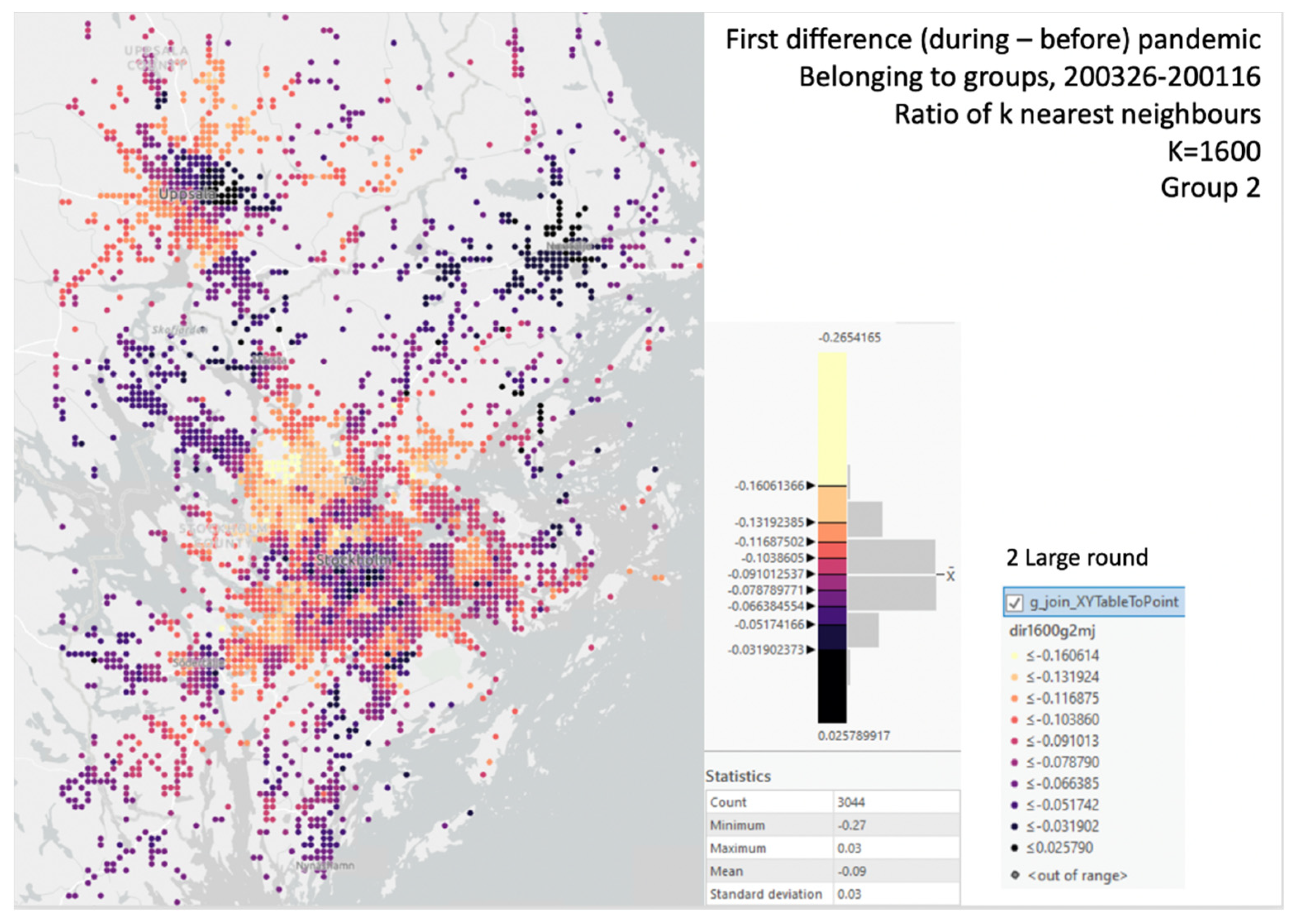
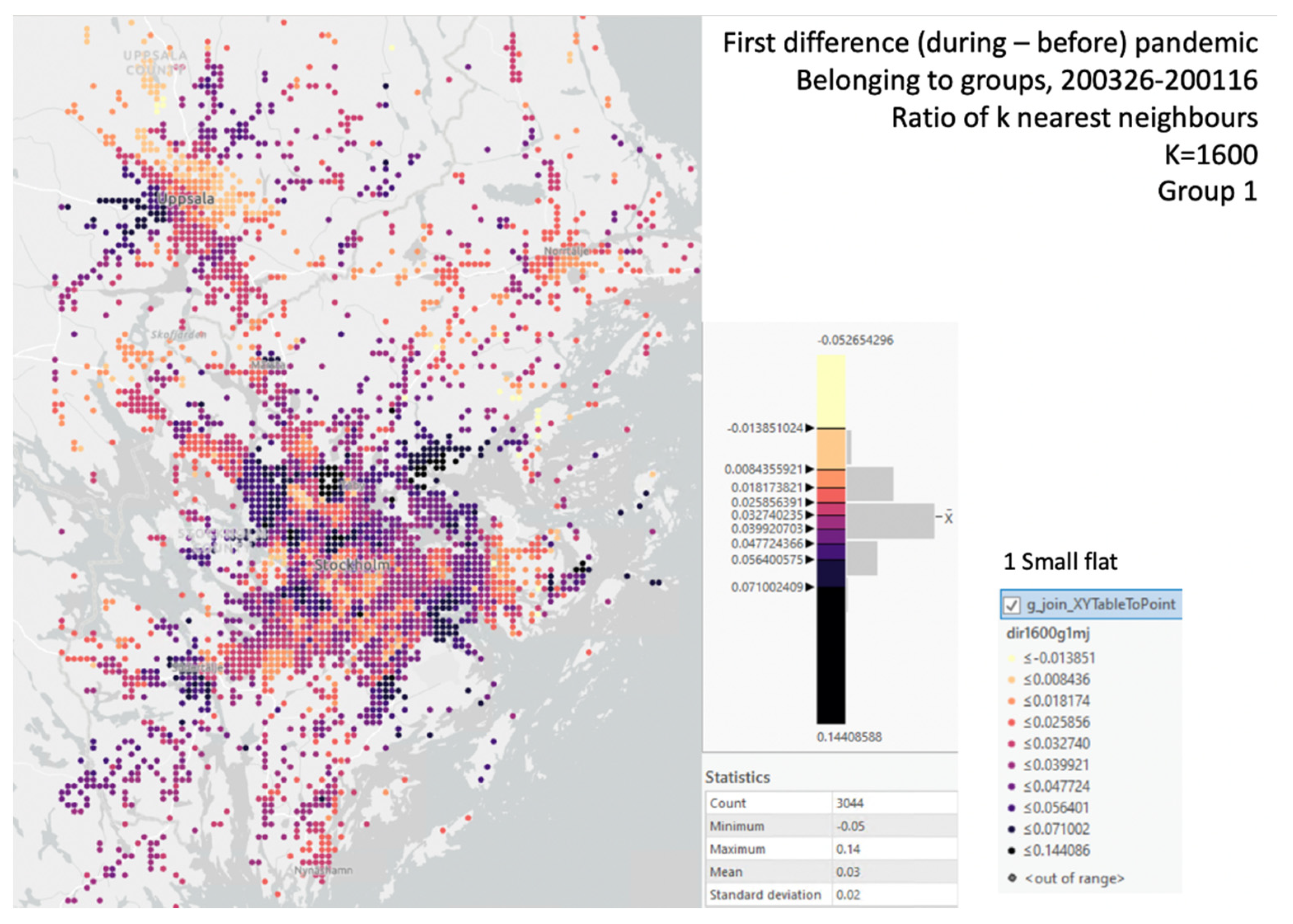
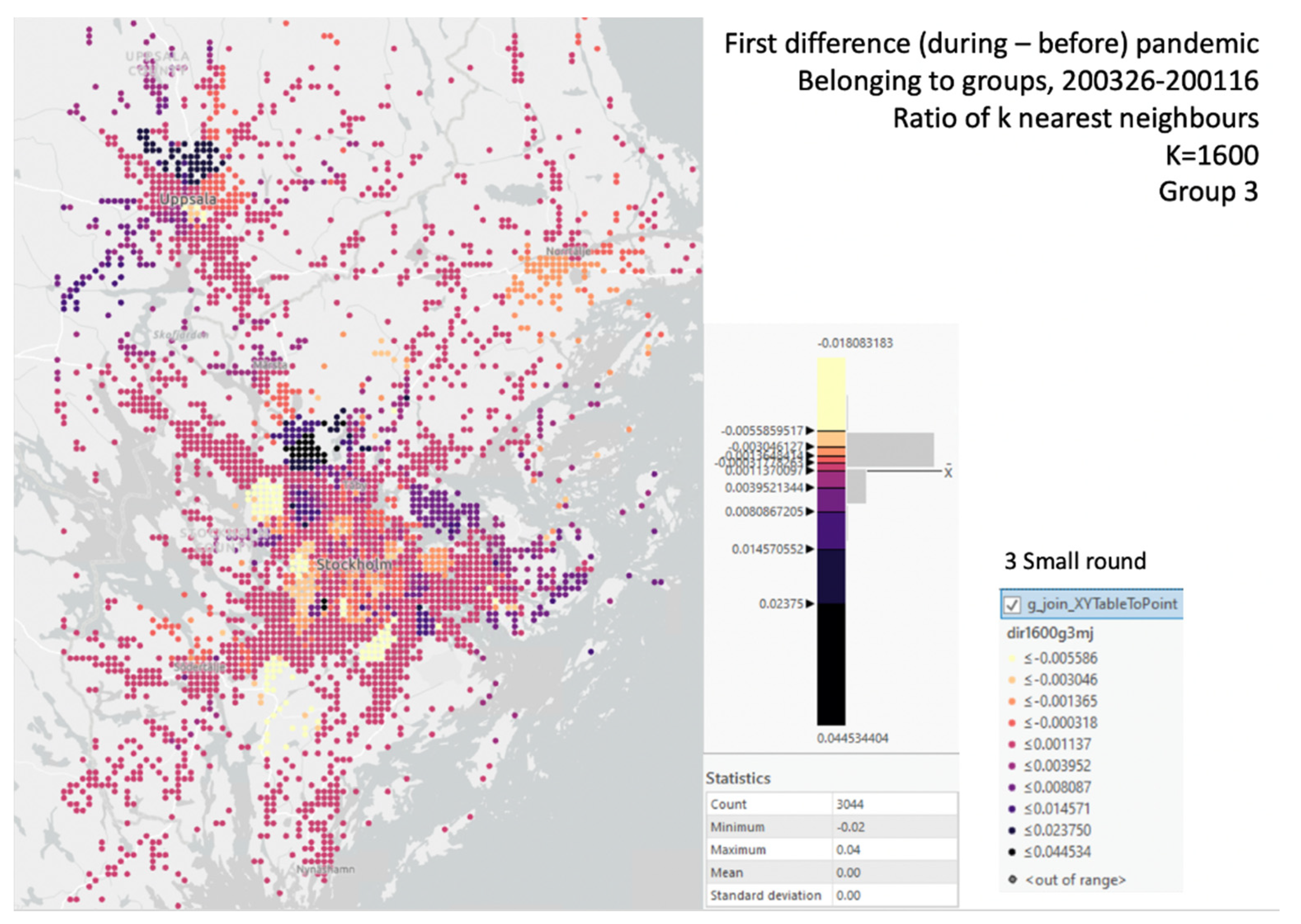
4.2. Socio-Demographics and Time Geography

It is clear that the changes in activity spaces is notable but also varying between different parts of the urban landscape. Since the urban landscape also have strong demographic variations, it is likely that the spatial patterns that was evident in previous parts if the paper is connected to local demographic characteristics. In the Table 4 we present the regression results for all the geometrical types.
The dependent variable holds aggregated values representing the over-time difference in the mean share of phone users that have a time-geographical activity space that are having a spatial behavior that can be represented by type 1 to 4 in corresponding models 1 to 4. The aggregated mean share represents the k = 800 nearest phone-users from the midpoint of each km2 unit, this to ensure that values from the two dates are as similar in composition as possible.
The explanatory variables are categorized in to three groups of function. In the first group, consisting of sociodemographic variables we see that areas with a greater share of higher educated individuals are becoming more associated with medium large and flat mobility patterns and less associated with flat geometries. Low education, on the other hand, is not associated with geometric flattening of the activity spaces. The only significant low-education result is a decrease of smaller circular activity spaces. Taken together, this suggest that lower educated areas are not having the same possibilities to telecommute as do higher educated individuals. The same pattern can be detected when we look at the relationship between poverty and geometry, and wealth and geometry. Poor areas are in fact associated with an increase of large round activity spaces and a reduction of the medium sized and flat activity spaces, while wealthy areas see a significant increase in small flat activity spaces (and a reduction in medium-sized flat). It is possible that the increased demand for home-delivery services and various other forms of gig-services has increased the need to travel in lower income areas. Finally, areas with higher shares of visible minorities (VM) see a reduction in type 2 activity spaces (large round activity spaces), and a significant increase in flat-geometric activity spaces. These patterns are consistent with commuting patterns for workers (and students, etc.) that must be at the workplace during work (working in shops, etc.), but that limits most other activities. The second group of variables are labor market related. With increasing distance to nearby jobs (k = 500 jobs in this variable) there is a decrease in larger circular geometries, but an increase in flat-geometric activity spaces. This pattern is similar to what was observed for higher educated areas. In the commuter towns and more distance suburbs (from especially Stockholm) villas, gardens and low job density can be associated with both longer distance to jobs and higher educated dwellers. Unemployment is associated with an increase in larger round activity spaces and a reduction in mid-sized flat ones. A possible explanation to the observed pattern is that job-matching is more difficult and requires individuals to commute longer. Finally, the two phone variables render inconclusive results, where both larger distances to k = 500 phones and increasing number of phones per km2 are associated with an increase in larger circular activity spaces and a small reduction smaller flat activity space. When we plot the results (not mapped) it becomes clear that the results support a U-curve interpretation where both long distances and larger local concentrations of jobs are associated with large and round geometries.

5. Conclusions

This preliminary study on the “new geography of corona” has explored the health risk related changes in mobility using the time geographical approach. The use of individual spatial mobility data allowed us to analyze in bulk the daily activity spaces of individuals using standard deviational ellipses (SDE). Aggregating these space-time profiles leads to a representative pattern of spatial location-allocation.
This study is showing that the COVID-19 pandemic has had a profound effect on the geometry of how we move during the course of a day. By departing from a time-geographical framework we study how the geometry of the activity spaces for more than 400,000 phones before and during the pandemic change, and if the shape change can be associated with behaviors that can be related with public recommendations for limiting the spread. Our results indicate that there is a substantial move from large and round activity spaces to more elliptic and smaller. However, our results also indicate that the change varies between geographical parts of our study region (the greater Stockholm region) and that change also is connected to the sociodemographic characteristics of the city. In short, the results indicate that suburban areas have altered their mobility patterns more than most other parts, and that variables such as income and education are good proxies for the ability to change mobility patterns.
It should be mentioned however that a time-geographical analysis of this magnitude requires longitudinal data repositories and a density of cell-towers and phone users that are difficult to obtain. Used data represent mobility patterns in the greater Stockholm region, but the relative scarcity of cell towers outside the metropolitan regions would make a similar study approach unreliable in rural or peri-urban parts of the country. Therefore, the study is limited to the dense urban regions. In addition, use of phones in Sweden is not restricted to specific ages (besides the very young) or socio-economic groups (market penetration of mobile phones in Sweden is 98%, [53]). However, on a global scale imbalance in phone usage may still pose a problem to representativeness of the time-geographical approach. Thus, the results may be generalizable in developed dense urban areas but less so in rural or developing regions.
Our research based on extensive Swedish data demonstrates the relevance of the time-geographical approach, echoing Klapka et al. [34]. The present study highlights how COVID-19 related changes of individual mobility have aggregate implications for the daily life of urbanites. Given our empirical findings, a range of mobility-related research issues is gradually coming to fore. The threat of density and spatial proximity means that spatial interaction in terms of frequency, scale, type, and intensity, will call for new research endeavors in the near future. The insight into the background forces and consequences of the observed or perceived negative externalities of the COVID-19 pandemic is needed, so as to trace not only short-term adjustments in mobility behavior, but also long-term adaptations in terms of spatial behavior, modal preferences, teleworking, and residential relocation choice. Consequently, the future of urbanization is at stake in the unprecedented age of the COVID-19 pandemic.

Author Contributions

Conceptualization, M.T., K.K., P.N. and J.Ö.; data curation, M.T. and J.Ö.; formal analysis, M.T. and J.Ö.; funding acquisition, M.T., K.K., P.N. and J.Ö.; investigation, M.T., K.K., P.N. and J.Ö.; methodology, M.T. and J.Ö.; project administration, K.K. and P.N.; resources, M.T. and J.Ö.; software, M.T. and J.Ö.; visualization, M.T.; writing—original draft, M.T., K.K., P.N. and J.Ö.; writing—review & editing, M.T., K.K., P.N. and J.Ö. All authors have read and agreed to the published version of the manuscript.

Funding

This research was funded by Axel and Margaret Ax:son Johnsons Foundation—invited grant “Urban-Environmental Presumptions of Public Life”, Sweden; FORMAS grant # 2018-00255; Romanian Ministry of Research and Innovation, CNCS—UEFISCDI, project number PN-III-P4-ID-PCCF-2016-0166. The APC was funded by MDPI.

Institutional Review Board Statement

This study is part of the project “Mobilitet i tid och rum” approved by the Ethics Committee of Uppsala—Regionala Etikprövningsnämnden Uppsala (Dnr 2017/205 from 2017-06-07).

Informed Consent Statement

Informed consent was obtained from the volunteers involved in the study.

Acknowledgments

We thank Alexey Siretskiy for technical help with data extraction; the Urban Lab at Uppsala University for support and inspiration; and we acknowledge the support of the funders: the Axel and Margaret Ax:son Johnsons Foundation, FORMAS, and the Romanian Ministry of Research and Innovation, CNCS—UEFISCDI.

Conflicts of Interest

The authors declare no conflict of interest.

Appendix A. Standard Deviational Ellipse (SDE)

To illustrate the relevance of a Standard Deviational Ellipse (SDE) approach for studying the COVID-19 pandemic related changes in the individual activity spaces, we map a GPS trajectory of the volunteer X (see Figure A1), followed by a presentation of their spatial pattern using Kernel Density (KD) as a simplification of the activity space (see Figure A2). Figure A1 shows a flat ellipse activity space for the SDE approach in case of going straight to work and a concentrated profile when working at home.
Figure A1. Standard deviational ellipse of the two trajectories of the volunteer X: the flat ellipse when commuting between home and work without additional stops (left) and small round ellipse when working from home (right). As a measure of activity space, it enables comparison of behaviors at an aggregate level with time dimension flattened (Uppsala, 2020).
Sustainability 13 04027 g0a1
As outlined above, another way to represent this spatial pattern of individuals would be to use Kernel Density (KD) estimations (see Figure A2).
Figure A2. Kernel Density as a way to flatten time. Activity space could be described as weighted sum of KD values. Note the differences between the bifocal distribution on a normal working day (left) versus the small concentrated on a pandemic working-from-home day (right).
Sustainability 13 04027 g0a2
The KD approach seemed promising, but in this study we opted for the SDE approach as in numerous other studies that use SDE as activity spaces [48] and also to make the computations scalable. We plan to continue with this analysis on multiple days in mass as an index of changing spatial behavior.

Appendix A.1. Calculating Activity Spaces Using a Standard Deviational Ellipse (SDE)

The next step is the calculation of the activity spaces. We follow the accepted procedure for calculating a standard deviational ellipse similar to the standard function in ArcGIS Pro [54]. Thus, we calculate the standard deviational ellipse as follows: S D E x and S D E y are coordinates of the ellipse centre.
S D E x = i = 1 n ( x i X ¯ ) 2 n ,   S D E y = i = 1 n ( y i Y ¯ ) 2 n
With coordinates of each location being x i , y i of n features, ellipse centre is located at the mean central location X ¯ ,   Y ¯ . The major axis is rotated at the angle calculated as:
tan θ = A + B C A = ( i = 1 n ( x i X ¯ ) 2   i = 1 n ( y i Y ¯ ) 2 ) B =   A 2 + C 2 C =   2 i = 1 n ( x i X ¯ ) ( y i Y ¯ )
standard deviations for the x and y axes are:
σ x = 2 i = 1 n ( ( x i X ¯ ) cos θ ( y i Y ¯ ) sin θ ) 2 n σ y = 2 i = 1 n ( ( x i X ¯ ) cos θ + ( y i Y ¯ ) sin θ ) 2 n
The variances for the axes are scaled (following the same logic as in [54]) by an adjustment factor in order to produce an ellipse (or ellipsoid in case of 3D) containing the desired percentage of the data points. These adjustment factors are provided in the Table A1 below.
Table A1. Scales for calculating ellipse axes variances.
1 Dimensional Data2-Dimensional Data3-Dimensional DataPercentage of Data Points
1 standard deviation1.001.411.7368%
2 standard deviations2.002.833.4695%
3 standard deviations3.004.245.2099%
The area of the ellipse was calculated using the ellipse axes: A =   π σ x σ y . The metrics to analyze the SDE flatness and size of the ellipse is given in Figure A3.
Below are the spatial distributions of activity spaces of type 1 (small and flat, 6.3% of all, Figure A4) and of type 3 (small and round, 0.3% of all, Figure A5).
Figure A3. Geometry of the ellipse: size (area) and flatness (ratio between major and minor axes); some illustrative metrics (a) and the actual trajectory-derived ellipses of volunteer X (b).
Sustainability 13 04027 g0a3
Figure A4. Spatial distribution of group 1 changes (first diff share of 1600 NN per km2).
Sustainability 13 04027 g0a4
Figure A5. Spatial distribution of group 3 changes (first diff share of 1600 NN per km2).
Sustainability 13 04027 g0a5

References

  1. Bailey, D.; Clark, J.; Colombelli, A.; Corradini, C.; De Propris, L.; Derudder, B.; Fratesi, U.; Fritsch, M.; Harrison, J.; Hatfield, M.; et al. Regions in a time of pandemic. Reg. Stud. 2020, 54, 1163–1174. [Google Scholar] [CrossRef]
  2. Florida, R.; Rodríguez-Pose, A.; Storper, M. Cities in a Post-COVID World; Papers in Evolutionary Economic Geography (PEEG) 2041; Utrecht University: Utrecht, The Netherlands, 2020; p. 29. [Google Scholar]
  3. Pullano, G.; Valdano, E.; Scarpa, N.; Rubrichi, S.; Colizza, V. Evaluating the effect of demographic factors, socioeconomic factors, and risk aversion on mobility during the COVID-19 epidemic in France under lockdown: A population-based study. Lancet Digit. Health 2020, 2, e638–e649. [Google Scholar] [CrossRef]
  4. Dahlberg, M.; Edin, P.-A.; Grönqvist, E.; Lyhagen, J.; Östh, J.; Siretskiy, A.; Toger, M. Effects of the COVID-19 pandemic on population mobility under mild policies: Causal evidence from Sweden. arXiv 2020, arXiv:2004.09087. [Google Scholar]
  5. Warren, M.S.; Skillman, S.W. Mobility changes in response to COVID-19. arXiv 2020, arXiv:2003.14228. [Google Scholar]
  6. Linka, K.; Goriely, A.; Kuhl, E. Global and local mobility as a barometer for COVID-19 dynamics. Biomech. Model. Mechanobiol. 2021, 20, 651–669. [Google Scholar] [CrossRef]
  7. Gao, S.; Rao, J.; Kang, Y.; Liang, Y.; Kruse, J. Mapping county-level mobility pattern changes in the united states in response to COVID-19. arXiv 2020, arXiv:2004.04544. [Google Scholar]
  8. Pase, F.; Chiariotti, F.; Zanella, A.; Zorzi, M. Bike sharing and urban mobility in a post-pandemic world. IEEE Access 2020, 8, 187291–187306. [Google Scholar] [CrossRef]
  9. Doubleday, A.; Choe, Y.; Isaksen, T.B.; Miles, S.; Errett, N.A. How did outdoor biking and walking change during COVID-19? A case study of three U.S. cities. PLoS ONE 2021, 16, e0245514. [Google Scholar] [CrossRef]
  10. Leyland, L.-A.; Spencer, B.; Beale, N.; Jones, T.; Van Reekum, C.M. The effect of cycling on cognitive function and well-being in older adults. PLoS ONE 2019, 14, e0211779. [Google Scholar] [CrossRef] [PubMed]
  11. SCB Sweden. Transport Sector Falls during the Coronavirus Crisis. Statistical News from Statistics Sweden 2020. Available online: https://www.scb.se/en/About-us/news-and-press-releases/transport-sector-falls-during-the-coronavirus-crisis/ (accessed on 20 January 2021).
  12. Hägerstrand, T. What about people in regional science? Pap. Reg. Sci. 1970, 24, 7–24. [Google Scholar] [CrossRef]
  13. Hacker, J.; Brocke, J.V.; Handali, J.; Otto, M.; Schneider, J. Virtually in this together—How web-conferencing systems enabled a new virtual togetherness during the COVID-19 crisis. Eur. J. Inf. Syst. 2020, 29, 563–584. [Google Scholar] [CrossRef]
  14. Östh, J.; Shuttleworth, I.; Niedomysl, T. Spatial and temporal patterns of economic segregation in Sweden’s metropolitan areas: A mobility approach. Environ. Plan. A Econ. Space 2018, 50, 809–825. [Google Scholar] [CrossRef] [Green Version]
  15. Östh, J.; Reggiani, A.; Schintler, L. Hierarchy, Central Place Theory and Computational Modelling. In Handbook on Entropy, Complexity and Spatial Dynamics: A Rebirth of Theory? Reggiani, A., Schintler, L., Czamanski, D., Partuelli, R., Eds.; Edward Elgar Publishing Ltd.: Cheltenham, UK, Forthcoming.
  16. Ratti, C.; Frenchman, D.; Pulselli, R.M.; Williams, S. Mobile landscapes: Using location data from cell phones for urban analysis. Environ. Plan. B Plan. Des. 2006, 33, 727–748. [Google Scholar] [CrossRef]
  17. Botta, F.; Moat, H.S.; Preis, T. Quantifying crowd size with mobile phone and Twitter data. R. Soc. Open Sci. 2015, 2, 150162. [Google Scholar] [CrossRef] [PubMed] [Green Version]
  18. Ellegård, K. Time Geography; Routledge Studies in Human Geography; Routledge: Abingdon, UK; New York, NY, USA, 2018; ISBN 978-1-138-57379-6. [Google Scholar]
  19. Wang, J.; Kwan, M.-P. Hexagon-based adaptive crystal growth voronoi diagrams based on weighted planes for service area delimitation. Int. J. Geoinf. 2018, 7, 257. [Google Scholar] [CrossRef] [Green Version]
  20. Wang, J.; Kwan, M.-P. An analytical framework for integrating the spatiotemporal dynamics of environmental context and individual mobility in exposure assessment: A study on the relationship between food environment exposures and body weight. Int. J. Environ. Res. Public Health 2018, 15, 2022. [Google Scholar] [CrossRef] [Green Version]
  21. Borsekova, K.; Nijkamp, P. Resilience and Urban Disasters: Surviving Cities; Edward Elgar Publishing: Cheltenham, UK, 2019; ISBN 1-78897-010-1. [Google Scholar]
  22. Jiang, S.; Yang, Y.; Gupta, S.; Veneziano, D.; Athavale, S.; González, M.C. The TimeGeo modeling framework for urban mobility without travel surveys. Proc. Natl. Acad. Sci. USA 2016, 113, E5370–E5378. [Google Scholar] [CrossRef] [PubMed] [Green Version]
  23. Kourtit, K.; Nijkamp, P.; Toger, M. Sustainable cities, quality of life and mobility-related happiness. In Urban Happiness; Springer International Publishing: Cham, Switzerland, Forthcoming.
  24. Hasanzadeh, K.; Czepkiewicz, M.; Heinonen, J.; Kyttä, M.; Ala-Mantila, S.; Ottelin, J. Beyond geometries of activity spaces: A holistic study of daily travel patterns, individual characteristics, and perceived wellbeing in Helsinki metropolitan area. J. Transp. Land Use 2019, 12. [Google Scholar] [CrossRef]
  25. Grinberger, A.Y.; Shoval, N.; McKercher, B. Typologies of tourists’ time–space consumption: A new approach using GPS data and GIS tools. Tour. Geogr. 2014, 16, 105–123. [Google Scholar] [CrossRef]
  26. Shoval, N.; McKercher, B.; Birenboim, A.; Ng, E. The application of a sequence alignment method to the creation of typologies of tourist activity in time and space. Environ. Plan. B Plan. Des. 2015, 42, 76–94. [Google Scholar] [CrossRef]
  27. Wang, Z.; He, S.Y.; Leung, Y. Applying mobile phone data to travel behaviour research: A literature review. Travel Behav. Soc. 2018, 11, 141–155. [Google Scholar] [CrossRef]
  28. Järv, O.; Ahas, R.; Witlox, F. Understanding monthly variability in human activity spaces: A twelve-month study using mobile phone call detail records. Transp. Res. Part C Emerg. Technol. 2014, 38, 122–135. [Google Scholar] [CrossRef]
  29. Chen, B.Y.; Wang, Y.; Wang, D.; Li, Q.; Lam, W.H.K.; Shaw, S.-L. Understanding the impacts of human mobility on accessibility using massive mobile phone tracking data. Ann. Am. Assoc. Geogr. 2018, 108, 1115–1133. [Google Scholar] [CrossRef]
  30. Osorio-Arjona, J.; García-Palomares, J.C. Social media and urban mobility: Using twitter to calculate home-work travel matrices. Cities 2019, 89, 268–280. [Google Scholar] [CrossRef]
  31. Raun, J.; Ahas, R.; Tiru, M. Measuring tourism destinations using mobile tracking data. Tour. Manag. 2016, 57, 202–212. [Google Scholar] [CrossRef]
  32. Kovács, Z.; Vida, G.; Elekes, Á.; Kovalcsik, T. Combining social media and mobile positioning data in the analysis of tourist flows: A case study from Szeged, Hungary. Sustainability 2021, 13, 2926. [Google Scholar] [CrossRef]
  33. Ellegård, K.; Svedin, U. Torsten Hägerstrand’s time-geography as the cradle of the activity approach in transport geography. J. Transp. Geogr. 2012, 23, 17–25. [Google Scholar] [CrossRef] [Green Version]
  34. Klapka, P.; Ellegård, K.; Frantál, B. What about time-geography in the post-Covid-19 era? Morav. Geogr. Rep. 2020, 28, 238–247. [Google Scholar] [CrossRef]
  35. Bin, E.; Andruetto, C.; Susilo, Y.; Pernestål, A. The trade-off behaviours between virtual and physical activities during the first wave of the COVID-19 pandemic period. Eur. Transp. Res. Rev. 2021, 13, 1–19. [Google Scholar] [CrossRef]
  36. Couclelis, H. Rethinking Time Geography in the Information Age. Environ. Plan. A Econ. Space 2009, 41, 1556–1575. [Google Scholar] [CrossRef]
  37. Nimrod, G. Technostress in a hostile world: Older internet users before and during the COVID-19 pandemic. Aging Ment. Health 2020, 1–8. [Google Scholar] [CrossRef]
  38. Mokhtarian, P. Teleworking and Mobility: What Do We (Think We) Know and Not Know? 2020. Available online: https://www.slideshare.net/OECDLEED/teleworking-and-mobility-what-do-we-think-we-know-and-not-know-patricia-mokhtarian (accessed on 20 January 2021).
  39. Couclelis, H. There will be no Post-COVID city. Environ. Plan. B Urban Anal. City Sci. 2020, 47, 1121–1123. [Google Scholar] [CrossRef]
  40. Hughes, C.J. Coronavirus escape: To the suburbs. The New York Times, 8 May 2020; 7. Available online: https://www.nytimes.com/2020/05/08/realestate/coronavirus-escape-city-to-suburbs.html(accessed on 20 January 2021).
  41. SCB Sweden. Real Estate Prices for One- or Two-Dwelling Buildings Rose in the Third Quarter 2020. Statistical news from Statistics Sweden 2020. Available online: https://www.scb.se/en/finding-statistics/statistics-by-subject-area/housing-construction-and-building/real-estate-prices-and-registrations-of-title/real-estate-prices-and-registrations-of-title/pong/statistical-news/real-estate-prices-and-registration-of-title-4th-quarter-of-2019/ (accessed on 20 January 2021).
  42. BBC Worklife Coronavirus: How the World of Work May Change Forever. BBC Worklife, Unknown Questions 2020. Available online: https://www.bbc.com/worklife/article/20201023-coronavirus-how-will-the-pandemic-change-the-way-we-work (accessed on 20 January 2021).
  43. Fairchild, C. WFH Is a Problem for Parents. Returning to the Office Won’t Solve It. Working Together, A Weekly Newsletter on Equity in the Workplace from LinkedIn News 2020. Available online: https://www.linkedin.com/pulse/wfh-problem-parents-returning-office-wont-solve-caroline-fairchild/work (accessed on 20 January 2021).
  44. Toger, M.; Shuttleworth, I.; Östh, J. How average is average? Temporal patterns in human behaviour as measured by mobile phone data—Or why chose Thursdays. arXiv 2020, arXiv:2005.00137. [Google Scholar]
  45. Thrift, N. An Introduction to Time-Geography: Concepts and Techniques in Modern Geography; Geo Abstracts Ltd.: Norwich, UK, 1977. [Google Scholar]
  46. Schaerström, A. The potential for time geography in health studies. In Geography and Health—A Nordic Outlook; The Swedish National Defence College: Stockholm, Sweden, 2015. [Google Scholar] [CrossRef]
  47. Wang, Y.; Kang, C.; Bettencourt, L.M.A.; Liu, Y.; Andris, C. Linked activity spaces: Embedding social networks in urban space. In Computational Approaches for Urban Environments; Helbich, M., Jokar Arsanjani, J., Leitner, M., Eds.; Springer International Publishing: Cham, Switzerland, 2015; pp. 313–336. ISBN 978-3-319-11468-2. [Google Scholar]
  48. Smith, L.; Foley, L.; Panter, J. Activity spaces in studies of the environment and physical activity: A review and synthesis of implications for causality. Health Place 2019, 58, 102113. [Google Scholar] [CrossRef] [PubMed]
  49. Schönfelder, S.; Axhausen, K.W. Activity spaces: Measures of social exclusion? Transp. Policy 2003, 10, 273–286. [Google Scholar] [CrossRef] [Green Version]
  50. Huang, X.; Li, Z.; Jiang, Y.; Li, X.; Porter, D. Twitter reveals human mobility dynamics during the COVID-19 pandemic. PLoS ONE 2020, 15, e0241957. [Google Scholar] [CrossRef] [PubMed]
  51. Östh, J. Introducing the EquiPop Software; Uppsala University: Uppsala, Sweden, 2014. [Google Scholar]
  52. Östh, J.; Türk, U. Integrating infrastructure and accessibility in measures of bespoke neighbourhoods. In Handbook of Urban Segregation; Edward Elgar Publishing: Cheltenham, UK, 2020; pp. 378–394. [Google Scholar]
  53. Davidsson, P.; Thoresson, A. IIS survey Swedes and Internet 2017. Available online: http://www.soi2017.se/allmant-om-utvecklingen/innehav-av-utrustning/ (accessed on 20 January 2021).
  54. Esri Inc. ArcGIS Pro; Esri Inc.: Redlands, CA, USA, 2020. [Google Scholar]
Figure 1. Observed mobility by mode in Sweden according to Apple Mobility Trends data (Change in routing requests since 13 January 2020, source: https://covid19.apple.com/mobility, accessed on 20 January 2021). Dates of this analysis are marked with arrows.
Sustainability 13 04027 g001
Figure 2. COVID-19 effects on individual activity spaces Comparison of a normal workday example of a couple with a pandemic workday (red and blue lines) with their respective activity spaces (blue and pink ellipse “shadows” on the “floor”): (a) normal day—one partner drives to work (blue line), drives to a lunch meeting and after work meets the other partner for dinner at a restaurant and then they drive home together. The other partner (red line) uses public transport to get to work (note the steeper slope as it takes longer time to cover the distances), then to class, then walks to the restaurant; (b) working day during the COVID-19 pandemic: one partner still commutes to work with the car (blue line) but has fewer movements and besides shopping on the way drives directly home. The other partner (red line) works from home. Both substitute meetings for digital interaction. Note the reduced activity spaces of both.
Sustainability 13 04027 g002
Figure 3. Illustration of time geography of a day’s trajectory: (a) an individual starts and ends at home, visiting several locations during the day (pre-pandemic); (b) a working day with starting at home (rightmost location), going to work (leftmost location) and getting back home at the end of the day. (c) Pandemic working from home trajectory.
Sustainability 13 04027 g003
Figure 4. Metrics of activity space per user: flatness of the ellipses and their size. The activity spaces became more flat and smaller, reflecting reduced mobility: (a) flatness of the ellipse measured by ratio of minor to major axes; (b) size of the ellipse measured by log 10 of square root of confidence 95% ellipse area.
Sustainability 13 04027 g004
Figure 5. Typologies of activity spaces, derived from the combination of flatness and size of the ellipse on a log scale. The abscissa represents flatness metric of ratio between minor and major axes of the ellipse (for reference a circle would have ratio of 1). The ordinate represents the size metric—square root of ellipse area in meters.
Sustainability 13 04027 g005
Figure 6. Spatial distribution of group 2 changes (first diff share of 1600 NN per km2).
Sustainability 13 04027 g006
Figure 7. Spatial distribution of group 4 changes (first diff share of 1600 NN per km2).
Sustainability 13 04027 g007
Table 1. Metrics of activity space per user—descriptive statistics.
VariableDatesMeanSDSEMinMdnMax
Each date
Ellipse area per phone, km22011646.63182.7740.21600.665136.99
2032630.32137.8040.27902.776850.03
Minor to major axes ratio201160.20710.20310.000400.141
203260.20320.21950.000300.151
Difference between dates
Ellipse area per phone, km220326-20116−9.02141.9110.248−4718.2−0.065070.4
Minor to major axes ratio20326-20116−0.00350.24840.0004−100.99
Table 2. Descriptors of groups.
grp1—Small Flat2—Large Round3—Small Round4—Medium FlatTotal
Perc.03268.862.70.328.2100
Perc.01166.372.10.321.3100
Table 3. Transition matrix between groups.
Transition Matrixgrp0326
grp01161 Small Flat2 Large Round3 Small Round4 Medium FlatTotal
1 small flat0.3380.0190.0930.0870.065
2 large round0.3900.8910.4070.5220.751
3 small round0.0060.0010.2530.0040.003
4 medium flat0.2660.0890.2470.3880.182
Total11111
Table 4. Regression results for groups 1–4; * = significant on 5% level, ** = significant on 1% level and *** = significant on 0.1% level.
(1)(2)(3)(4)
Beta (S.E.)SignBeta (S.E.)SignBeta (S.E.)SignBeta (S.E.)Sign
Dependent Variable:
First Diff in Share 800 NN
Group g1 Small FlatGroup g2 Large RoundGroup g3 Small RoundGroup g4 Medium Flat
Sociodemographics
Higher education0.021879 (0.0085) *−0.099 (0.014) ***−0.004131 (0.0027)0.081516 (0.0111) ***
Lower education0.007872 (0.0157)−0.025 (0.026)−0.015297 (0.005) **0.031979 (0.0205)
VM0.041475 (0.0086) ***−0.147 (0.014) ***0.004015 (0.0027)0.101914 (0.0112) ***
Poverty−0.014983 (0.0174)0.175 (0.029) ***0.000182 (0.0055)−0.160255 (0.0226) ***
Wealth0.036343 (0.0106) ***0.025 (0.018)−0.004769 (0.0034)−0.056144 (0.0138) ***
Labour market
Distance to 500 jobs0.000001 (0) ***−0.003331 (0) ***0.000000 (0)0.000002 (0) ***
Local jobs−0.000002 (0)0.005759 (0) **0.000000 (0)−0.000004 (0) **
Unemployment−0.006296 (0.0218)0.087 (0.036) *−0.009839 (0.0069)−0.071034 (0.0285) *
Phone variables
Distance to 500 phones−0.000002 (0) ***0.003066 (0) **0.000000 (0) *−0.000001 (0)
phone density per km2−0.000001 (0) **0.001508 (0) **0.000000 (0) *−0.000001 (0)
(Constant)0.019194 (0.0037) ***−0.069 (0.006) ***0.006183 (0.0012) ***0.043863 (0.0048) ***
adj. R20.0460.1060.1000.080
Publisher’s Note: MDPI stays neutral with regard to jurisdictional claims in published maps and institutional affiliations.

