Digital Plan of Brickwork Layout for Robotic Bricklaying Technology

Abstract

The trend of using modern technologies in the construction industry has been growing stronger recently, particularly in the fields of additive construction or robotic bricklaying. Therefore, specifically for the purpose of robotic bricklaying, we created a digital layout plan for robotic construction works. This article presents a universal methodology for creating a bricklaying plan for various variations of wall building systems. The method is based on the conversion of drawings from the BIM (Building Information Model) environment to the BREP (Boundary Representation) model through use of the IFC (Industry Foundation Classes) format, which simultaneously divides object models into layers and connects discontinuous wall axes by means of an orthogonal arrangement and inserting details into critical structural points. Among other aspects, the developed algorithm proposes the optimal placement of the robotic system inside objects under construction, in order to minimize the distance of the robot’s movement and to reduce its electricity consumption. Digital layout plans created in this way are expected to serve as a stepping stone for robotic bricklaying.

1. Introduction

At present, the deployment of robots and intelligent systems is experiencing rather swift development, according to the Industry 4.0 methodology, not only in mechanical engineering, but also in other sectors of the economy. Due to the difficulty of implementing robotic systems in dynamic construction environments, the construction industry traditionally falls behind the engineering industry in this regard. The aim of this article is to present a method to create a digital layout plan for robotic bricklaying works. The idea to devise a method enabling the creation of digital bricklaying layout plans arose while working on a project, where the goal was to build an object from ceramic blocks using a KUKA industrial robot [1,2]. When searching the Espacenet (European Patent Office) [3] database for the keywords “brick” and “robot”, 4673 results were found. Careful examination of selected robotic systems revealed that none of them referred to a reliable method of transporting objects from the BIM environment to the industrial robot environment [4]. In this type of software, walls are displayed only as compact objects, in which openings for doors and windows can be created, but it is not possible to split the walls into individual building elements [5,6,7]. In order to be able to use an industrial robot for bricklaying, it is necessary to obtain detailed information about each element in the structure, such as the position of the respective elements in the structure, dimensions of the elements, their physical properties and shape, how the individual elements are connected, the places from which elements will be taken, how they will be transported into the structure and, finally, it is also important to know what connecting materials will be used for bricklaying, in what form the connecting material is most often supplied, and how it is to be applied [8,9]. Therefore, we decided to devise a methodology for creating a digital bricklaying plan based on BIM data. This research holds great promise for future applications and, thanks to its further development, it will also be possible to apply the procedures identified here to other robotic construction works, such as finishing works, plastering, painting, robotic realization of paving and tiling, etc. After digitization of construction works, it is possible to use or adjust mathematical optimization methods to suggest the optimal design of work procedures and, as a result, to reduce the time of the deployment of robotic systems, as well as reducing energy consumption and CO₂ emissions [10,11].

2. Methodology

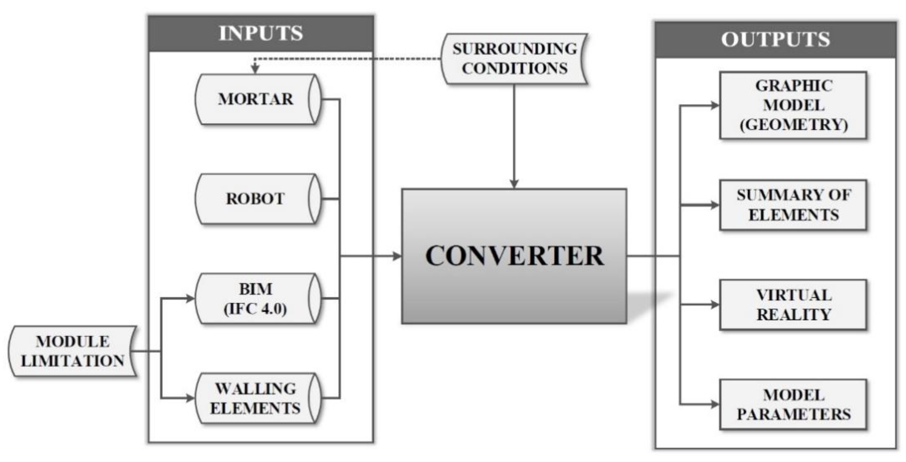
This part of the article focuses on the data necessary for the creation of a digital brickwork layout plan for the robotic bricklaying technology and on the method to convert these data into the desired outputs. Figure 1 displays the flowchart for the digital brickwork layout plan, where all input data (stored in a previously compiled database) can be seen on the left side of the diagram [12,13].

The first input data in Figure 1 are walling elements, which can be found in the database of different brick elements. The database of walling elements contains the manufacturer, type of material of elements, material structure, whether the element is used for load-bearing or non-load-bearing brickwork, dimensions, weight, and heat transfer coefficients. According to the pre-defined geometric parameters and the type of structure, a 3D model is automatically created for each walling element. Three types of details that can be typically found in structures using these elements are also created in the database for each walling element: Corner detail, T-joint detail, and jamb detail. The geometric layout of elements used for the details are mostly included in the technical sheets supplied by the brickwork system manufacturer [14]. As can be seen in Figure 1, a module limitation for walling elements applies here [15]; that is, it is necessary to think about what element will be used in correspondence with the drawing made in the BIM environment [16]. Thus, it applies here that, if a walling element with a building module of 250 mm is chosen, the height of the fabricated wall should be a multiple of this module. The inside geometric plan dimension of the room or the inside wall axis should also be a multiple of the module [17]. 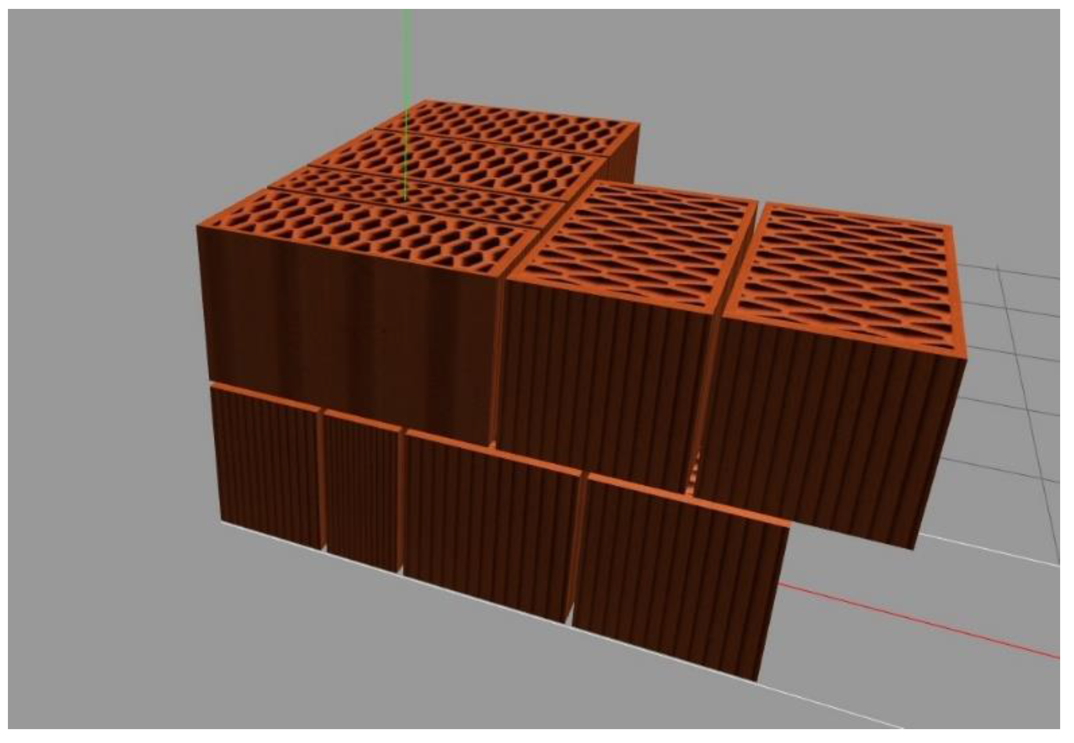Figure 2 shows the detailed assembly of a corner in the Porotherm 44 Profi building system. In Figure 2, the first two rows of the corner and all used blocks can be seen, including special corner brick blocks. This detail and the details of other building systems have been uploaded to the database, in order to increase versatility and simplify the work.

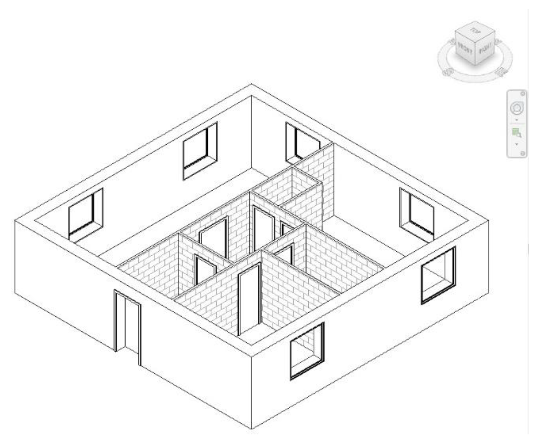
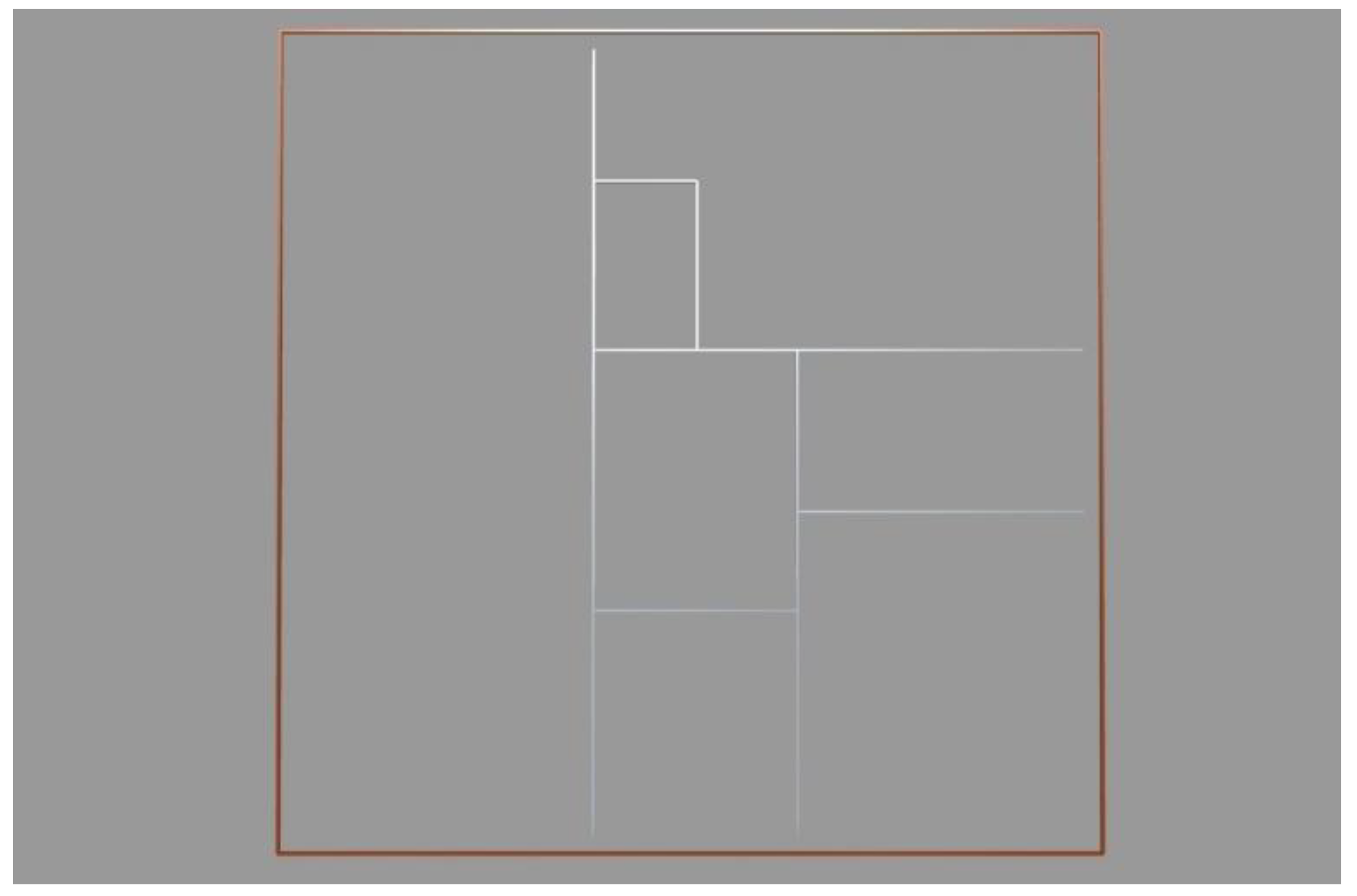
The same applies to a drawing in the BIM environment: If a wall 3 m high is to be built, an adequate walling element must be chosen for it; hence, an element with a building module of 250, 200, or 500 mm could be selected for this wall. This leads us to a drawing in the BIM environment where a model of an object can be made, for example, by using special software [5,6,18,19]. This model should only be designed to the height of the upper edge of the lintel over the openings, as shown in Figure 3. This model is subsequently converted and exported into the universal IFC 4.0 format [20,21,22].

Other input data on the left side of Figure 1 are robot parameters. Here, the parameters of robots, which can be chosen from a previously compiled database, are uploaded. The parameters are the maximum and minimum reach of the robot, its load capacity, weight, speed, output, etc. [23,24,25].

A database of adhesive mixtures has also been compiled for mortars, from which we can choose. The parameters specified for each mortar are compressive strength, maximum and minimum processing temperatures, necessary amounts of water, package weight, density, product price, etc. As the diagram in Figure 1 shows, the limiting conditions are surrounding conditions. This means that there is a temperature limitation for mortars, restricting when they can be processed. The condition for the processing temperature range serves in the automatic calculation of the duration of walling processes for a specific geographic area [26]. All input information, such as that related to the mortar, robot, BIM, and building elements, as described above, is entered into the converter, which converts them in several steps into the desired outputs using the methods described in Section 3.

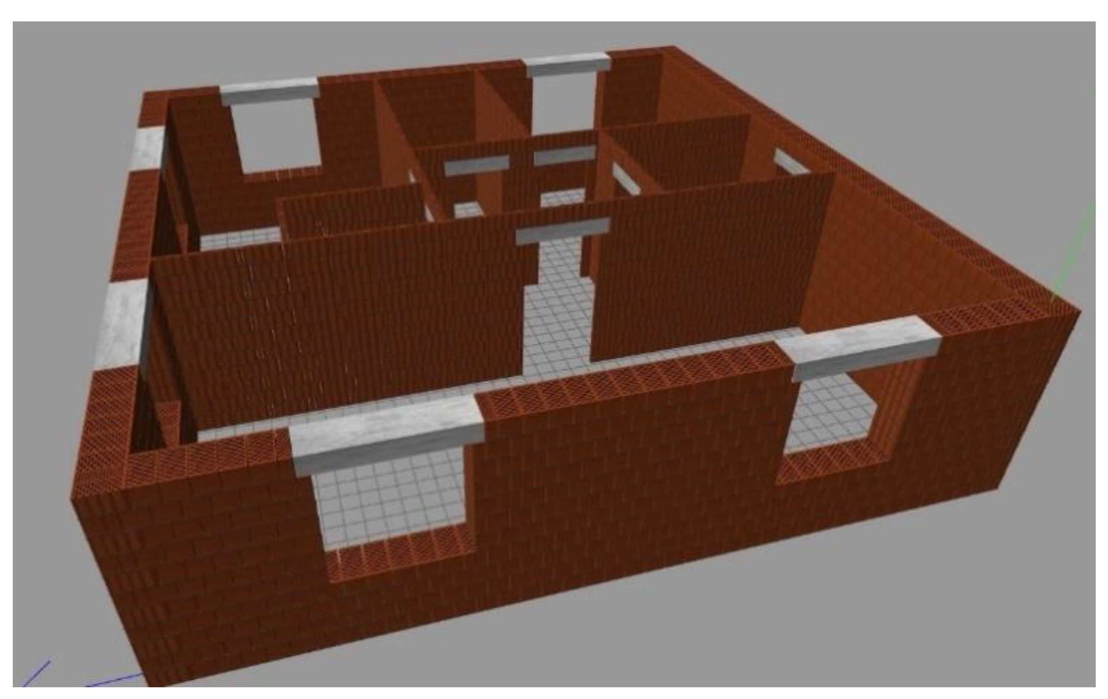
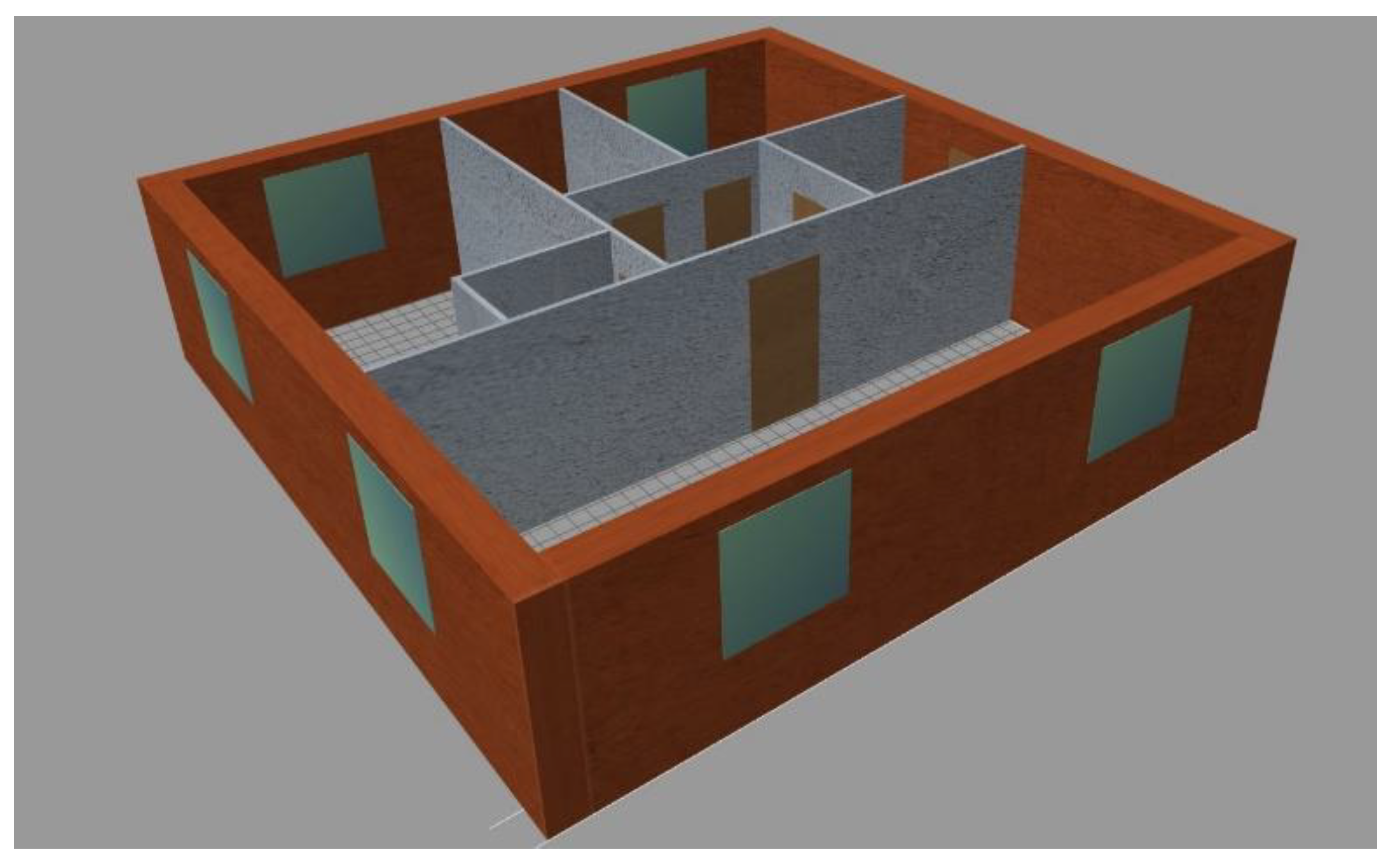
The first output is a graphic model with information about each walling element, which is part of the object. Each element has a precise position, type, dimensions, angular rotation in space, and an order in the digital plan. This model is interactive, such that the user can walk through it, rotate it, move individual elements in the structures, and swap them. Figure 4 displays a sample model. As can be seen in the figure, all structural elements in the model are drawn as separate 3D models and have a material structure corresponding to the selected walling element [27,28,29].

Another output is the summary of elements, where all elements from the graphic model are described in the list. Each brick is described there, along with the order in which it was laid in the structure and which row, as well as basic information about the walling elements. The information about the chosen mortar and its use is also added [30,31].

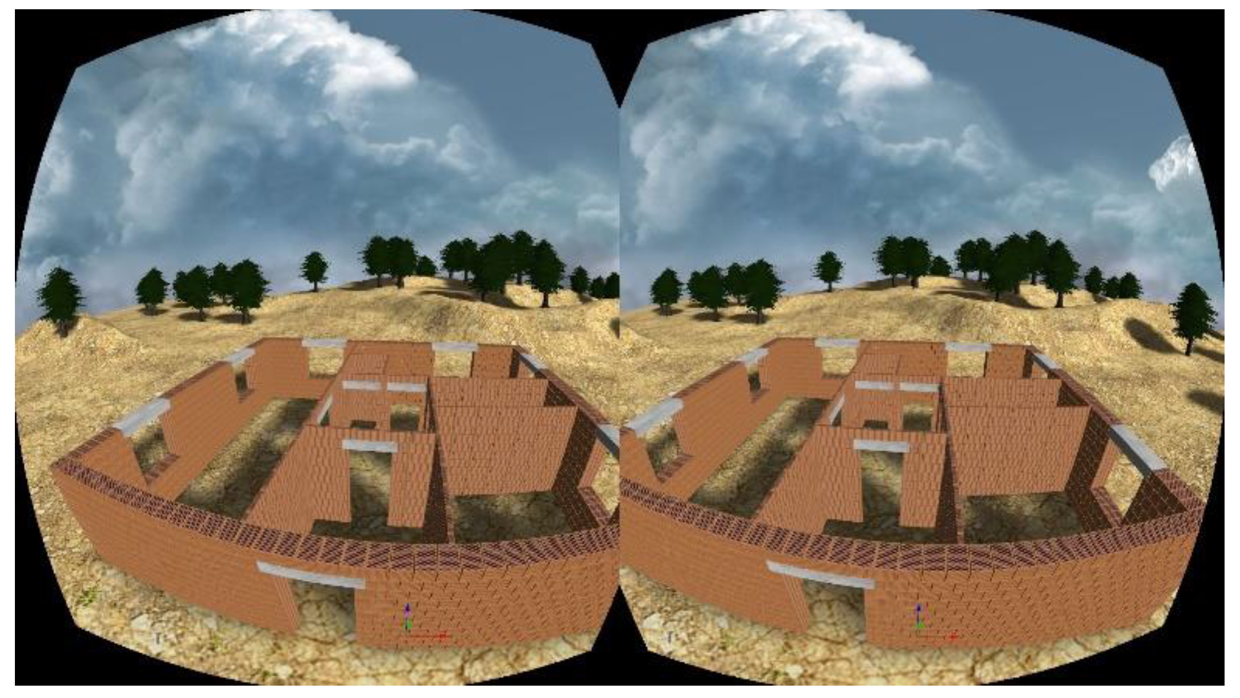
The third output is VR (virtual reality), allowing the graphic model in Figure 4 to be virtually walked through. This model is interactive. Equipped with goggles, a module for virtual reality [32], and a web interface [33], users can be placed inside the object, and can walk from one room to another, around the object, and pass through doors. We can also take elements out of the structure, rotate them, and even move them. It must also be mentioned that the elements moved in virtual reality are updated in the graphic model and the model itself is be updated, which is one of the steps contributing to progress towards the “Industry 4.0” paradigm [34,35]. A view through virtual reality goggles is shown in Figure 5.

The final outputs are model parameters, which are available in the system from the calculated model, including a chart of brickwork classification by its structure, cost distribution, division of elements into the load-bearing and non-load-bearing systems, time consumption chart, number of used elements, and even the construction time of such an object by a robot [36,37,38].

3. Algorithm of the Converter from IFC Format

This chapter presents the system algorithm, which converts the model in IFC 4.0 format into the graphic model divided into individual walling elements [21].

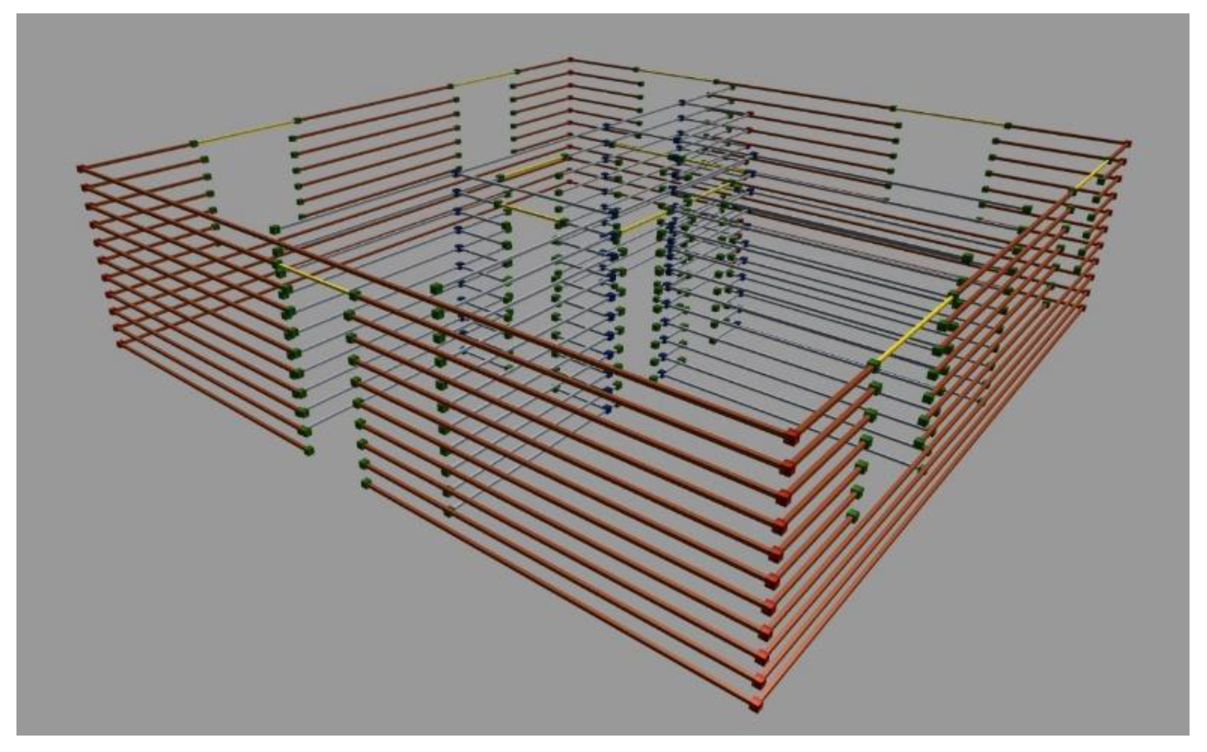
Step 1: In the first step, load-bearing and non-load-bearing walls are converted from IFC format to a BREP model, including windows and doors. In place of windows and doors, only the BREP location of openings are maintained; see Figure 6.

The basic intermediate steps are described in

Table 1. The basic intermediate steps of parsing the IFC (Industry Foundation Classes) file.

Intermediate Steps	Visualization of Conversion
Reading from IFC file and searching for wall object	159 IFCSHAPEREPRESENTATION(#102,‘Body’,‘SweptSolid’,(#149)); 162 IFCPRODUCTDEFINITIONSHAPE($,$,(#141,#159)); 166 IFCWALLSTANDARDCASE(‘1JhL2KuR9Fthk9hVMuZzBg’, #41, ‘Non-bearing wall: Porotherm 8:318893’,$,‘Non-bearing wall:Porotherm 8:318625’,#135,#162,‘318893’); 175 IFCMATERIAL(‘Brick wall’); 180 IFCSTYLEDITEM($,(#178),$); 182 IFCSTYLEDREPRESENTATION(#97,‘Style’,‘Material’,(#180));
Parsing object and searching for other properties	166: IFCWALLSTANDARDCASE, #41, $, #135, #162 135: IFCLOCALPLACEMENT, #122, #134 134: IFCAXIS2PLACEMENT3D, #132, #19, #17 132: IFCCARTESIANPOINT, −8320.17111815646, 16161.2332918, 0. 17: IFCDIRECTION, 0., −1., 0. 162: IFCPRODUCTDEFINITIONSHAPE, $, $, #141, #159 159: IFCSHAPEREPRESENTATION, #102, #149 149: IFCEXTRUDEDAREASOLID, #147, #148, #19, 2750. 147: IFCRECTANGLEPROFILEDEF, .AREA., $, #146, 9500., 79.999
Translated and rotated co-ordinates for each wall object	Type of object: non-bearing wall IFC Raw: 166 Geometry of object (length/width/height in mm): 9500/80/2750 Co-ordinate axis: middle Rotation (degree): 270 Co-ordinates of object start: −8320;16161 Co-ordinates of object end: −8320;6661

, for the example of a conversion of one wall to a geometric object for further modelling. first, it is necessary to read the IFC file, then to parse it into a wall object and convert IFC objects to geometric objects with translated and rotated co-ordinates [21].

Step 2: The next step is the division of the object into layers, according to the used walling element height module. This parameter is chosen while drawing the model and selecting the walling element. For our sample model, this basic module was 250 mm. The result of the model division into layers is displayed in Figure 7.

Step 3: In this step, the axes of the walls are connected, as the software in which it is possible to model the BIM environment cannot connect the object axes, which are drawn separately at first [5,6,19,39]. This step will be described in detail in Section 4. Figure 8 shows Step 3.

In Step 4, critical points to which details are assigned are localized. Details are found for each layer of the object divided in Step 2. The types of details are successively assigned to a specific point in the structure and can be in three versions: Corner, jamb, and T-joint (see Figure 9). These details are prepared in advance, in the compiled database of walling elements. Details in the model are displayed in the form of points with different colors, according to the type of detail.

Step 5: In the next step, load-bearing and non-load-bearing walls are filled with standard elements, inserted between mounted details. Lintels in load-bearing walls are also laid over window and door openings. Figure 10 displays details inserted at the points found in Step 4. Standard elements are inserted between details in Figure 10, which is the last modification of the graphic model of an object [40].

Step 6: Step 6 is the final step of the algorithm, in which it is possible to view the entire graphical model of the object with all inserted elements. The model shown in Figure 4 is the final output of this algorithm. This model can be converted to a list format of elements for further calculations, such as optimal use of space or optimal placement of a pallet with bricks to reduce the movement of the robotic arm and reduce the total construction time of the robotic masonry [41,42]. This is discussed further in Section 5.

4. Mathematical Method of Connecting Discontinuous Axes of Objects Walls with an Orthogonal Layout

When examining existing mathematical methods for connecting orthogonal axes, several mathematical algorithms were identified, such as those presented in [43] or [44]. Each of the methods is capable of reliably determining the intersection of discontinuous axes with rapid convergence using basic mathematical procedures. However, the actual application of the procedures already developed for digitizing the wall bricklaying plan (converter between the BIM environment and industrial robots) is very limited (or even completely non-viable), due to the specific method of deployment. Our algorithm is able to reliably divide objects into load-bearing and non-load-bearing elements. Optimization computations are affected by other limiting conditions, such as the width of walls, the connection of the object walls according to the details described, and the location of windows and doors in the object. An integral part of the restrictive conditions stems from the technological requirements of building systems manufacturers [14]. This research study describes the methodology using already known mathematical methods for a specific purpose. The input geometry of a sample object is schematically displayed in Figure 11.

Basic steps of the algorithm for connecting $i$-discontinuous axes:

Step 1: Determine the end points of the axes of object walls $P_{1i}\left[x;y\right]$ and $P_{2i}\left[x;y\right]$, where $i\in {\mathbb{N}}^{+}$ and $x,y\in ℝ$.

Step 2: Conversion of the axes of object walls to parametric form, as follows:

• Find the directional vector $\overrightarrow{b}$ for each axis:

  $$\overrightarrow{b}= \left[b_1;b_2\right]= P_{2i}- P_{1i}=\left[x_2-x_1;y_2-y_1\right].$$

  (1)
• Find the initial point, $S$, for each axis $a$:

  $$S\left[x_0;y_0\right]= P_{1i}\left[x;y\right].$$

  (2)
• Write the axes in parametric form, as a system of equations [45]:

  $$\{\begin{array}{c}x= x_0+ b_1·t\\ y= y_0+ b_2·t\end{array}$$

  (3)
• Write the axes $a$ in matrix form [45]:

  $$a_i= \left(\begin{array}{cc}{x}_0& b_1\\ y_0& b_2\end{array}\right),$$

  (4)

  where $a_i\in {ℝ}^2$ and $i\in {\mathbb{N}}^{+}$, wherein $a_i\left(S;\overrightarrow{b}\right)=\left\{S_i+{\overrightarrow{b}}_i·t | t\in ℝ\right\}$, where $S$ is the initial point on the line $a$ and $\overrightarrow{b}$ is the directional vector of the line $a.$

Step 3: Write the co-ordinates of the intersections of discontinuous axes of the object in the matrix form, where the matrix $C= {\left(c_{i,j}\right)}_{n,n}$ is the upper triangular (square) matrix with main diagonal equal to zero ($c_{i,i}=\varnothing$), $n$ is the number of axes in the object,$c\in {ℝ}^2$, and $i,j\in {\mathbb{N}}^{+}$:

$$C= \left(\begin{array}{ccccc}\varnothing & c_{1,2}& c_{1,3}& \dots & c_{1,i}\\ \varnothing & \varnothing & c_{2,3}& \dots & c_{2,i}\\ \dots & \dots & \varnothing & \dots & \dots \\ \dots & \dots & \dots & \varnothing & c_{i-1,i}\\ \varnothing & \varnothing & \dots & \dots & \varnothing \end{array}\right)$$

(5)

where $c_{i,j}=\varnothing$ in the case that the axes (lines) do not have an intersection (are parallel or identical) or $c_{i,j}=\left[x_c;y_c\right]$ in the case that the axes (lines) have an intersection.

The parallelism and identity of the two axes $i$ and $j$ are checked as follows. Two linear equations have the form:

$$\{\begin{array}{c}{P}_i=P_{1i}+t_i·\left(P_{2i}-P_{1i}\right)\\ P_j=P_{1j}+t_j·\left(P_{2j}-P_{1j}\right)\end{array}$$

(6)

where points $P_{1i}$ and $P_{2i}$ are the initial and end points of axis $i$ and $P_{1j }$ and $P_{2j}$ are the initial and end points of axis $j$, respectively. After solving a system of equations under the condition of finding a common intersection of the axes $P_i=P_j$ and obtaining the $x$ and $y$ co-ordinates, we receive:

$$\{\begin{array}{c}{P}_{1ix}+t_i·\left(P_{2ix}-P_{1ix}\right)=P_{1jx}+t_j·\left(P_{2jx}-P_{1jx}\right)\\ P_{1iy}+t_i·\left(P_{2iy}-P_{1iy}\right)=P_{1jy}+t_j·\left(P_{2jy}-P_{1jy}\right)\end{array}$$

(7)

By solving the system for $t_i$ and $t_j$, two formulae are obtained:

$$\{\begin{array}{c}{t}_i=\frac{\left(P_{2jx}-P_{1jx}\right)·\left(P_{1iy}-P_{1jy}\right)-\left(P_{2jy}-P_{1jy}\right)·\left(P_{1ix}-P_{1jx}\right)}{\left(P_{2jy}-P_{1jy}\right)·\left(P_{2ix}-P_{1ix}\right)-\left(P_{2jx}-P_{1jx}\right)·\left(P_{2iy}-P_{1iy}\right)}\\ t_j=\frac{\left(P_{2ix}-P_{1ix}\right)·\left(P_{1iy}-P_{1jy}\right)-\left(P_{2iy}-P_{1iy}\right)·\left(P_{1ix}-P_{1jx}\right)}{\left(P_{2jy}-P_{1jy}\right)·\left(P_{2ix}-P_{1ix}\right)-\left(P_{2jx}-P_{1jx}\right)·\left(P_{2iy}-P_{1iy}\right)}\end{array}$$

(8)

If the denominator in the formulae is equal to zero, the axes are parallel to each other ($i\left|\right|\mathrm{j}$). If both the numerator and the denominator in the formulae are equal to zero, the axes are identical ($i=\mathrm{j}$).

Three versions may occur when the denominator differs from zero:

• Both parameters $t_i$ and $t_j$ lie in the interval $\langle 0, 1\rangle$ and the intersection of the axes is found between the end points of the axes, which does not comply with the conditions for drawing objects; hence, $c_{i,j}=\varnothing$.
• Neither $t_i$ nor $t_j$ lies in the interval $\langle 0, 1\rangle$ and the intersection of the axes is found outside the axis area delimited by the end points of the axes, which does not comply with the conditions for drawing objects; hence, $c_{i,j}=\varnothing$.
• Only one of $t_i$ or $t_j$ lies in the interval $\langle 0, 1\rangle$ and the intersection of the axes is found between the end points on one axis and outside the area delimited by the end points on the second axis, which complies with the conditions for drawing objects. Hence, the co-ordinates of the intersection of the axes are calculated using the formulae below; that is, $c_{i,j}=\left[x_{ijc};y_{ijc}\right]$, where

  $$\{\begin{array}{c}{x}_{ijc}=P_{1ix}+t_i·\left(P_{2ix}-P_{1ix}\right)\\ y_{ijc}=P_{1iy}+t_i·\left(P_{2iy}-P_{1iy}\right)\end{array}$$

  (9)

  or

  $$\{\begin{array}{c}{x}_{ijc}=P_{1jx}+t_j·\left(P_{2jx}-P_{1jx}\right)\\ y_{ijc}=P_{1jy}+t_j·\left(P_{2jy}-P_{1jy}\right)\end{array}.$$

  (10)

Step 4: The distances determined between the end points of the axes and their intersection are written in matrix form, where the matrix $D= {\left(d_{i,j}\right)}_{n,n}$ is the upper triangular (square) matrix with main diagonal equal to zero $d_{i,i}=\varnothing$, where $n$ is the number of axes in the object and $d\in \left(\left|d_1\right|;\left|d_2\right|;\left|d_3\right|;\left|d_4\right|\right)$, $i,j\in {\mathbb{N}}^{+}$ and $\left|d_1\right|,\left|d_2\right|\left|d_3\right|\left|d_4\right|\in ℝ$ are the distances between the intersection and the end points of the axes:

$$D= \left(\begin{array}{ccccc}\varnothing & d_{1,2}& d_{1,3}& \dots & d_{1,i}\\ \varnothing & \varnothing & d_{2,3}& \dots & d_{2,i}\\ \dots & \dots & \varnothing & \dots & \dots \\ \dots & \dots & \dots & \varnothing & d_{i-1,i}\\ \varnothing & \varnothing & \dots & \dots & \varnothing \end{array}\right),$$

(11)

where it holds true for each $c_{i,j}=\varnothing ⟹d_{i,j}=\varnothing$ and for each $c_{i,j}\ne \varnothing ⟹d_{i,j}=\left(\left|d_{1i,j}\right|;\left|d_{2i,j}\right|;\left|d_{3i,j}\right|;\left|d_{4i,j}\right|\right).$

The distance in the plane between the intersection and the end points of the axes can be found using the formulae:

$$\{\begin{array}{c}\left|d_{1i,j}\right|=\sqrt{{\left(x_{ijc}-P_{1ix}\right)}^2+{\left(y_{ijc}-P_{1iy}\right)}^2}\\ \left|d_{2i,j}\right|=\sqrt{{\left(x_{ijc}-P_{2ix}\right)}^2+{\left(y_{ijc}-P_{2iy}\right)}^2}\\ \left|d_{3i,j}\right|=\sqrt{{\left(x_{ijc}-P_{3ix}\right)}^2+{\left(y_{ijc}-P_{3iy}\right)}^2}\\ \left|d_{4i,j}\right|=\sqrt{{\left(x_{ijc}-P_{4ix}\right)}^2+{\left(y_{ijc}-P_{4iy}\right)}^2}\end{array}$$

(12)

Step 5: Next, we check the existence of the possibility of connecting the axes, based on the condition of the maximum distance between the intersection and the end point of the axis. A reduction is made to the matrix $D\to D^{\prime }$ of permissible states. Two admissible states can occur in the algorithm:

• Corner connection of the axes (see Figure 11, State 1), under the condition:

  $$\left\{\left|d_{1i,j}\right|\vee \left|d_{2i,j}\right|\right\}=\left\{\left|d_{3i,j}\right|\vee \left|d_{4i,j}\right|\right\}=\frac{w}{2}$$

  (13)

  where w is the width of the object wall.
• T-connection of the axes (see Figure 11, State 2) under the condition:

  $$\left\{\left|d_{1i,j}\right|\vee \left|d_{2i,j}\right|\vee \left|d_{3i,j}\right|\vee \left|d_{4i,j}\right|\right\}=\frac{w}{2}$$

  (14)

Step 6: In the next step, a correction of the end points of the axes is made:

• For the corner connection of axes (see Figure 12, State 1):

  $$\{\begin{array}{c}\left\{P_{1i}\left[x;y\right]\vee P_{2i}\left[x;y\right]\right\}= \left[x_c;y_c\right]\\ \left\{P_{3i}\left[x;y\right]\vee P_{4i}\left[x;y\right]\right\}= \left[x_c;y_c\right]\end{array}.$$

  (15)
• For the T-connection (see Figure 12, State 2):

  $$\left\{P_{1i}\left[x;y\right]\vee P_{2i}\left[x;y\right]\right\}\vee \left\{P_{3i}\left[x;y\right]\vee P_{4i}\left[x;y\right]\right\}=\left[x_c;y_c\right]$$

  (16)

Step 7: In the last step, the modified end points of the axes of object walls, $P_{1i}\left[x;y\right]$ and $P_{2i}\left[x;y\right]$, are formulated, where $i\in {\mathbb{N}}^{+}$ and $x,y\in ℝ$.

5. Experimental Verification and Practical Demonstration of Research

The functionality of the algorithm was verified during the deployment of a robotic system currently in development within the scope of the project TH04010329, “Autonomous robotic construction system”. The main goal of the project is to develop a functional prototype of an autonomous robotic construction system, enabling accurate and fast construction production with a reduced number of construction workers. The system focuses on precise bricklaying on mortar (i.e., foundations, load-bearing, and dividing walls). Based on the object construction documentation (BIM), the autonomous system (with the help of a built-in converter) exports the construction model to the interface of the industrial robot, which subsequently carries out the construction process [46,47].

The robotic system is based on an industrial six-axis robot [1] consisting of several parts: An industrial robot with a reach of 3900 mm and a load capacity of 120 kg, a load base, a universal end tool for attaching bricklaying blocks of various sizes and shapes made from standard building materials, and supporting equipment for vacuum production and signal processing. The universal end tool is equipped with a system for applying a bricklaying adhesive and also contains several laser sensors, enabling the correct and precise placement of bricklaying elements, according to the co-ordinates from the digital layout plan. 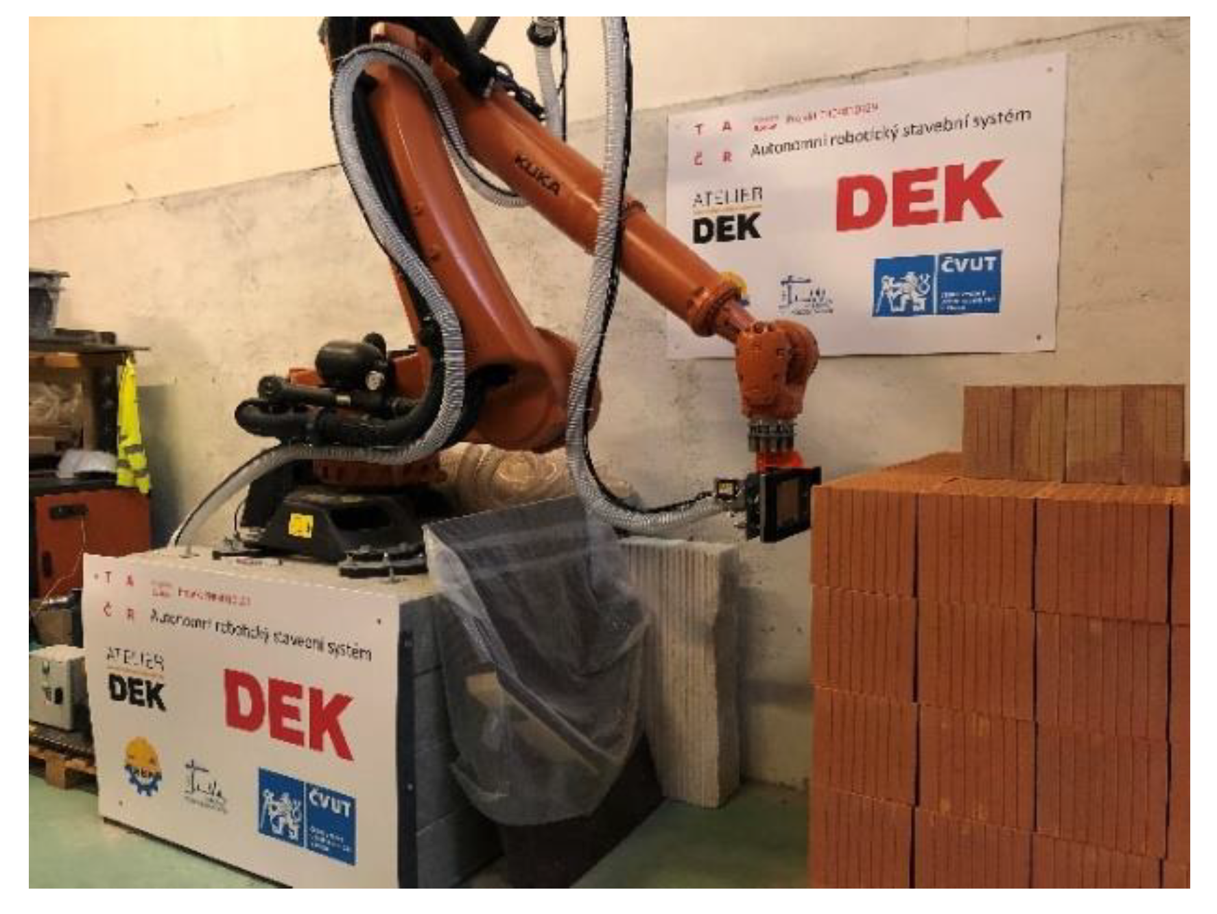The model of the system, including a sample of the brick wall and supply pallets, is shown in Figure 13. The actual prototype of the system is shown in Figure 14.

To verify the functionality of our algorithm, the following steps were performed: Conversion and adjustment of partial construction objects (i.e., walls, doors, and windows) from the BIM environment to the BREP model, including the application of the algorithm to connect the axes.

For the investigated object in Figure 3, the state before the connection of the axes is represented in

Table 2. Input basic geometry and location of object axes in space.

ID	IFC	Length, [mm]	Width, [mm]	Height, [mm]	Axis	Axis Rotation, [grad]	Axis Beginning, [X;Y]	Axis End, [X;Y]
1	560	9500	440	2750	middle	90	220;440	220;9940
2	527	9940	440	2750	middle	180	9940;220	0;220
3	494	9940	440	2750	middle	270	10160;9940	10160;0
4	445	10380	440	2750	middle	0	0;10160	10380;10160
5	405	1250	80	2750	middle	0	4060;8340	5310;8340
6	371	2380	80	2750	middle	0	4060;3150	6440;3150
7	337	5810	80	2750	middle	270	6480;6250	6480;440
8	303	3420	80	2750	middle	180	9940;4340	6520;4340
9	269	5880	80	2750	middle	0	4060;6290	9940;6290
10	235	1970	80	2750	middle	270	5270;8300	5270;6330
11	166	9500	80	2750	middle	270	4020;9940	4020;440

. The state after the connection of the axes is represented in

Table 3. Output basic geometry and location of object axes in space.

ID	Length, [mm]	Width, [mm]	Height, [mm]	Axis Rotation, [grad]	New Length, [mm]	Axis Start, [X;Y]	Axis End, [X;Y]	New Axis Start, [X;Y]	New Axis End, [X;Y]
1	10380	440	2750	0	9940	0;10160	10380;10160	220;10160	10160;10160
2	9940	440	2750	270	9940	10160;9940	10160;0	10160;10160	10160;220
3	9940	440	2750	180	9940	9940;220	0;220	10160;220	220;220
4	9500	440	2750	90	9940	220;440	220;9940	220;220	220;10160
5	9500	80	2750	270	9500	4020;9940	4020;440	4020;9940	4020;440
6	1970	80	2750	270	2050	5270;8300	5270;6330	5270;8340	5270;6290
7	5880	80	2750	0	5920	4060;6290	9940;6290	4020;6290	9940;6290
8	3420	80	2750	180	3460	9940;4340	6520;4340	9940;4340	6480;4340
9	5810	80	2750	270	5850	6480;6250	6480;440	6480;6290	6480;440
10	2380	80	2750	0	2460	4060;3150	6440;3150	4020;3150	6480;3150
11	1250	80	2750	0	1250	4060;8340	5310;8340	4020;8340	5270;8340

. Note that the ID numbering of the axes will change during the algorithm, according to the order of the walling technological processes.

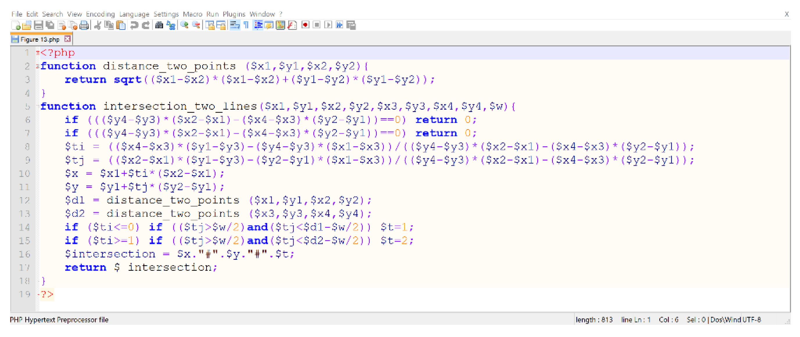
In Figure 15, a practical example of the source code of finding the intersections of the axes in the PHP programming language is displayed [48].

In the following step, the object under construction was divided into partial bricked elements (e.g., details, load-bearing, and non-load-bearing walling).

Part of a full list of bricks is represented in

Table 4. List of brick elements, with co-ordinates and other parameters.

Order	Wall	Description	Length, [mm]	Width, [mm]	Height, [mm]	Position of Center, [X;Y;Z]	Layer	Rotation	Weight, [kg]
1	Bearing	Porotherm 44 Profi K	250	440	250	220;9815;125	1	180	21.1
2	Bearing	Porotherm 44 Profi	250	440	250	220;9565;125	1	180	20.4
3	Bearing	Porotherm 44 Profi R	187	440	250	93.5;10160;125	1	90	15.4
4	Bearing	Porotherm 44 Pro 1/2	125	440	250	249.5;10160;125	1	90	11.0
…	…	…	…	…	…	…	…	…	…
2230	Non-bearing	Porotherm 8 Profi	500	80	250	4020;2360;2625	11	180	9.4
2231	Non-bearing	Porotherm 8 Profi	500	80	250	4020;1860;2625	11	180	9.4
2232	Non-bearing	Porotherm 8 Profi	500	80	250	4020;1360;2625	11	180	9.4
2233	Non-bearing	Porotherm 8 Profi	500	80	250	4020;860;2625	11	180	9.4
2234	Non-bearing	Porotherm 8 Profi	170	80	250	4020;525;2625	11	180	3.2

, showing the co-ordinates and final placement of each brick, brick type, geometric parameters, descriptions of elements, number of layers, rotations in the main co-ordinate system, and the weight of elements. This complete information is fully sufficient for operating the robotic system and can easily be updated or transformed to the KRL program language for KUKA robots or other systems [49].

In the final step, the necessary optimal location for the robotic system is selected, in order to enable the bricklaying work to be realized in the entire building, including load-bearing and non-load-bearing masonry. Optimally determined locations for the robotic unit must ensure complete bricklaying in the object; at the same time, their proper identification reduces the distance of the relocation route for bricklaying elements, as well as the time of the execution of technological bricklaying processes. Application of the method developed will also reduce the amount of energy required for the robotic system to operate.

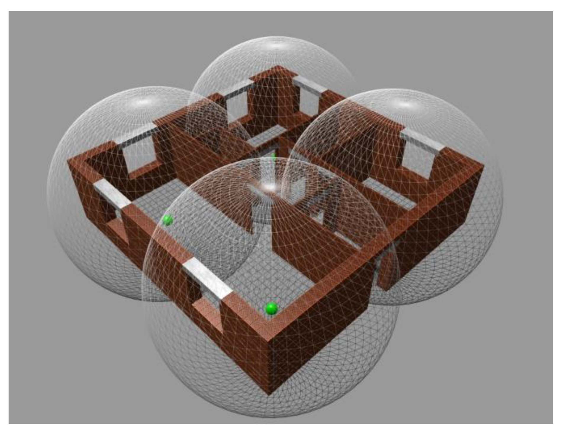
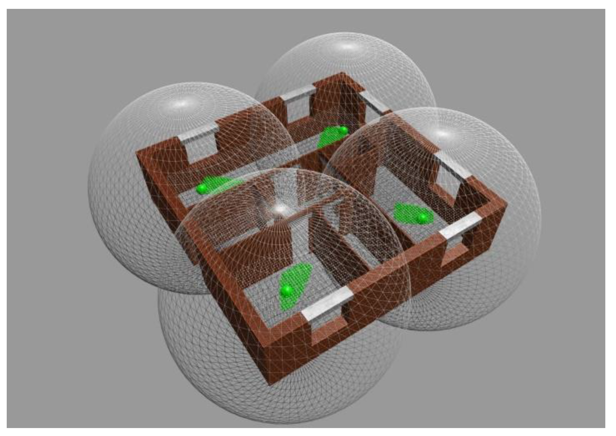
Obviously, a robotic system based on an industrial robot has its limitations. The operating space is located between two spheres: The minimum possible range and the maximum possible range. For the developed system, the maximum range is based on the operational reach of the KUKA Quantic KR120 R3900 robotic arm, which has a radius equal to 3900 mm from the center of the robot’s location. The robot used has a cantilever arrangement and the reach of its robotic arm is increased by placing the robot in the middle of the wall height. In the case of the test object, the vertical movement of the robot center was 1375 mm. The sphere of the minimum range is based on the technical documentation of the manufacturer [1]. The robotic unit was transported to a designated location with the help of a crane, followed by the assembly, fixing, and calibration of the system.

In the first sub-step of calculating the optimal location of the robotic unit, a number of construction points are suggested for the system to achieve complete bricklaying technological processes: Depalletization, rectification, exact placement of elements in the building structure according to calculated co-ordinates, application of bricklaying adhesive, and laser sensor check of the object (see Figure 16). The minimum number of construction points for the object was set to four. The initial position of the robot was determined by the center of the quadrants of the object.

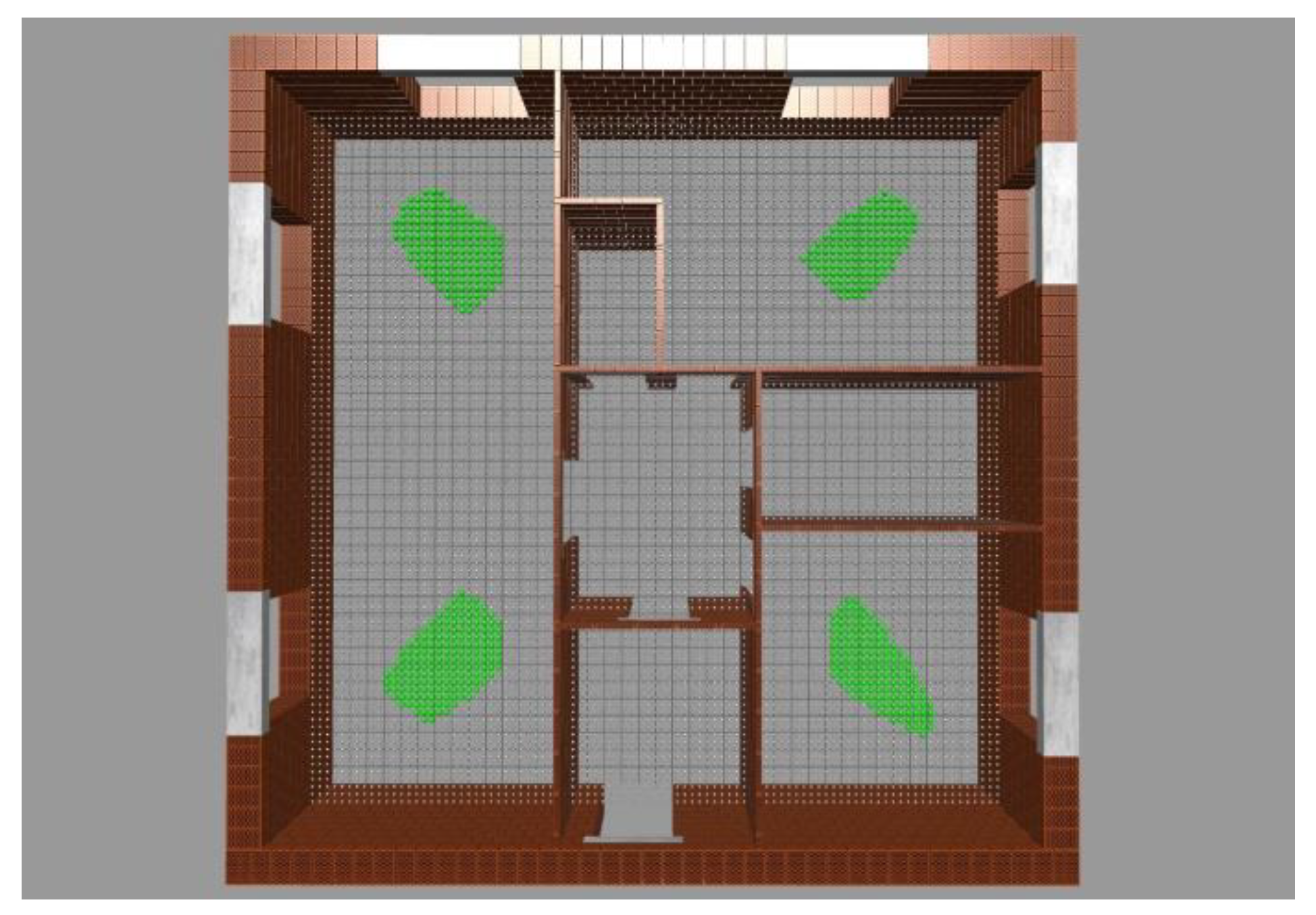
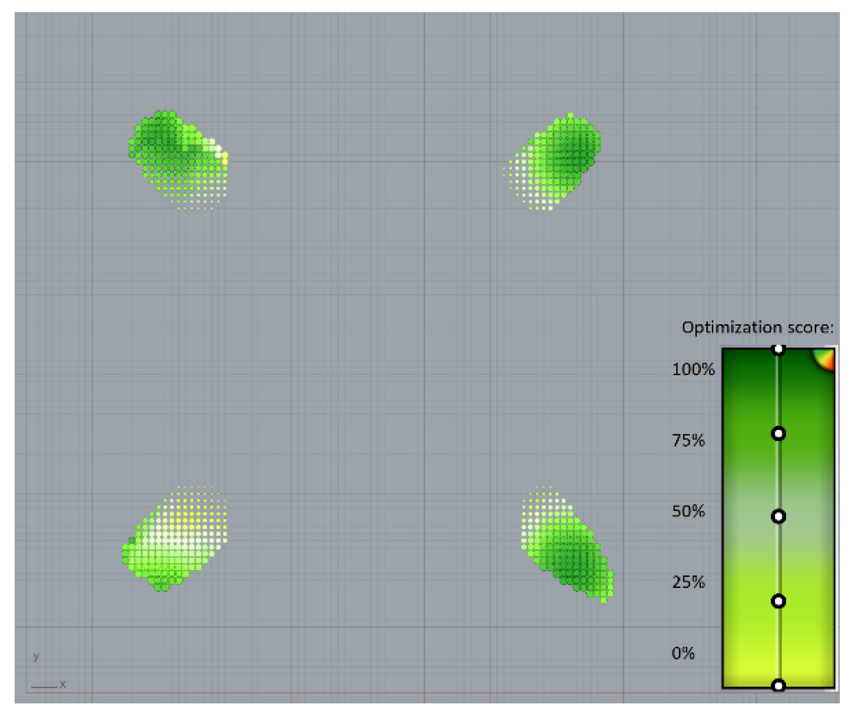
In the second sub-step, a set of possible positions for the robotic unit location was determined for each of the construction points. The following inputs were used to determine the admissible set: The co-ordinates of building components (walls, windows, doors) and the parameters of the robotic unit (minimum and maximum possible ranges). According to the BREP model, limiting vertices and local co-ordinate maxima were determined for each masonry element of the building. A grid with a mesh size of 100 mm was superposed on the floor plan of the building, at the height of the robotic unit location. The denser the grid, the more computational time is needed for the optimization calculation; however, at the same time, better results can be achieved. The mesh size of 100 mm ensures relatively optimal results with a maximum deviation of 5% from the very best solution. However, the result can be calculated in a very short time (within 5 s for 4 locations and 17 partial building objects). Subsequently, an admissibility check was performed for each grid point, and an admissible set of points was determined for further calculation (see Figure 17).

In the case of the test object, the total number of all possible positions was equal to 8649. After checking the maximum and minimum reach of the particular robotic unit, the number of positions was reduced to 637, in accordance with

Table 5. Determination of admissible set of positions for robotic unit.

Location	Initial Co-Ordinates, [X;Y;Z] in mm	Initial Amount of Examined Points	Number of Admissible Points
1	2500;2500;1375	2209	176
2	2500;7500;1375	2162	176
3	7500;7500;1375	2116	137
4	7500;2500;1375	2162	148

.

In the last sub-step, the calculation of the total route movement of the robot is performed for each admissible point of the set of optimal positions of the robotic unit (green points in Figure 17). The input for the calculation consists of the co-ordinates of one acceptable position of the robotic unit and the set of points of all building elements (i.e., co-ordinates, location, shape, and size of the elements) in the objects in which bricklaying is to be performed from the corresponding position. The route of movement of the robotic unit is calculated as the sum of the movements needed for each bricklaying element, ranging from the supply pallet constantly located next to the robotic unit, up to the target placement of the bricklaying element in the building, in accordance with the digital bricklaying plan output. A centering table will always stand in the path of the movement of bricklaying elements, as it is needed to check the grip control and the integrity of the bricklaying element. Therefore, the same portion of the route for each acceptable location of the robotic unit can be subtracted from the optimization calculation. Only the route from the center of the robot (location of the robotic unit/green dot in Figure 17) to the target location in the wall is included in the optimization calculation. Part of the final calculation of the movement route for the TCP (Tool Centre Point) robot is shown in

Table 6. Computing the movement route of robotic unit TCP (Tool Centre Point) for admissible points in the first location.

Point	Co-ordinates, [X;Y;Z] in mm	Total Distance of TCP Movement, [mm]
1	1500;2000;1375	1,230,399
2	1500;2100;1375	1,240,776
3	1500;2200;1375	1,252,321
…	…	…
174	3000;2700;1375	1,338,326
175	3000;2800;1375	1,401,561
176	3000;2900;1375	1,420,925

.

For the first location, 176 points were included in the set of admissible robot positions. The optimal point for the first placement location was identified at the co-ordinates [2000;1600;1375], where the total route of the TCP movement was 1192 m, according to the minimization criterion. The deviation between the maximum and minimum values of the total route of the TCP movement for the first location was equal to 9.56%. For each location, the calculation was performed identically and the optimal points of the robotic unit location for the entire object were determined (see Figure 18). The optimization algorithm performed 19,321,866 steps to detect the optimal positions for each location. It can be stated that the optimization method used to determine suitable locations for the robot unit, according to the criterion of minimizing the total route of the TCP movement, can lead to a reduction in the total movement trajectory of the given object, ranging from 6 to 12%. The final location of the robotic system is shown in Figure 19.

Table 7. Optimal position of robotic unit and estimated reduction of TCP total movement route.

Location	Optimal Position, [X;Y;Z] in mm	Minimum Movement Route of TCP, [m]	Maximum Movement Route of TCP, [m]	Initial Movement Route of TCP, [m]	Total Reduction of Route Distance
1	2200;1600;1375	1192	1467	1306	9.56%
2	2200;8700;1375	1392	1584	1504	8.05%
3	8300;8100;1375	1585	1675	1643	3.65%
4	8200;1900;1375	1564	1703	1629	4.16%
	Total:	5733	6429	6082	6.09%

shows the reduction of the necessary relocation and the total route of the TCP robot, both for the entire object under examination and for its individual locations.

Finally, the analysis of energy consumption is performed, in order to assess the amount of energy needed for robotic construction of the object examined.

6. Discussion

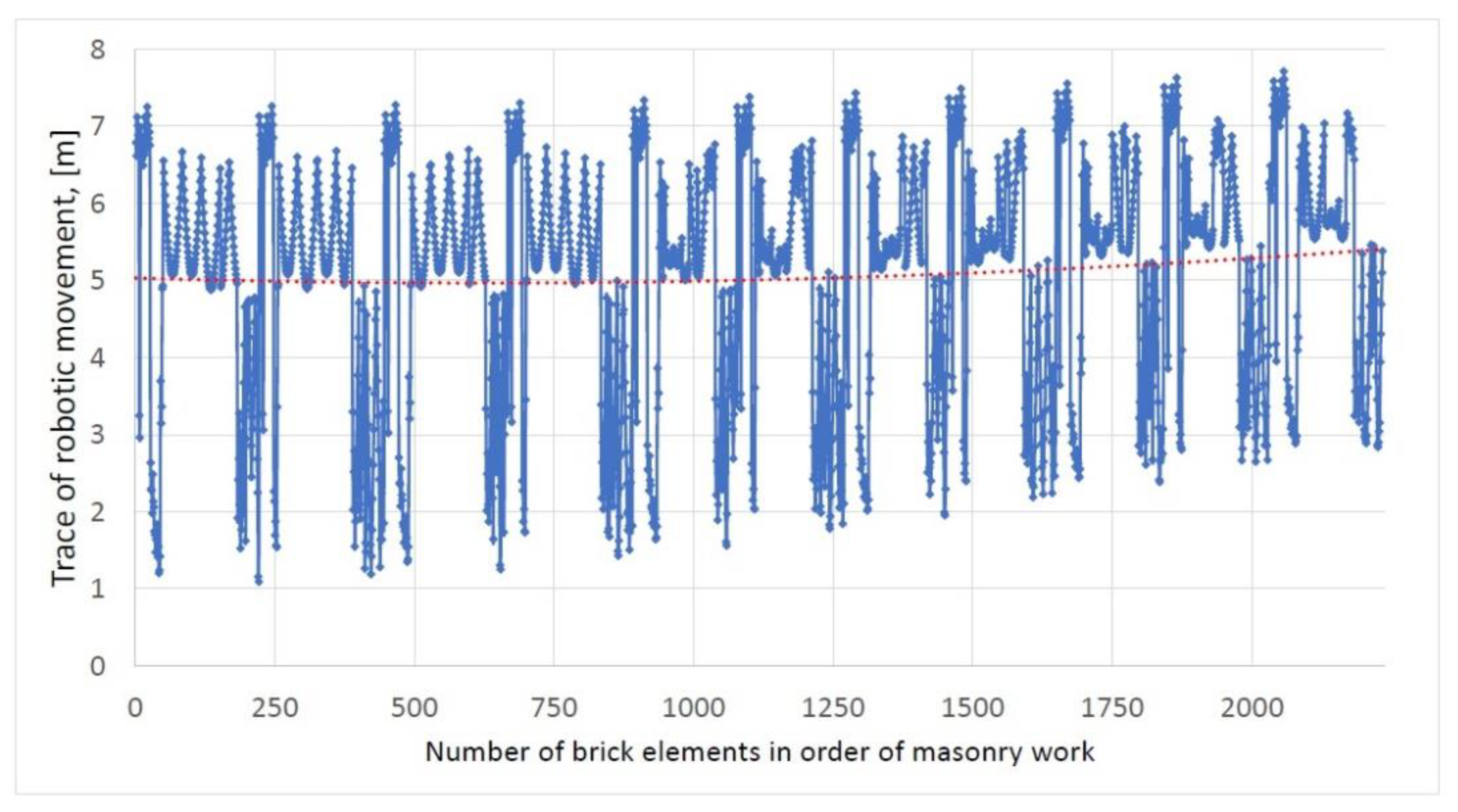
The results of this research work are suitable for further use and applications when working with autonomous robotic construction systems. The main benefit lies in the possibility of optimizing the movement of the robotic arm and using the co-ordinates of building elements to be able to remove them from the pallet with precision and then place them into the proposed structure. The proposed system is an effective helper in designing buildings, namely thanks to the converter, which is able to decompose various shapes of structures into the required building elements. Further optimization of the placement of pallets with building elements could reduce the overall distance of the robotic movement and reduce the wear on the entire robotic autonomous system. The reduction of the total TCP movement route leads to less wear of the motors and gearboxes of the robotic system. Figure 20 shows the optimized distances between the center of the robotic unit locations and the target location of each building element in the object. Future steps may involve calculating and minimizing the wear of each motor and gearbox of the robotic arm.

As can be seen from the practical example described in Section 5, the algorithm developed reduced the overall movement of the robotic arm by 6–12%, in contrast with the non-optimized option. Newer robotic industrial robots and systems already have built-in monitoring protocols for energy consumption analysis. KUKA robots based on the KR C4 controller have active variables in the monitoring mode for energy consumption analysis (e.g., $CURR_ACT) [2,49]. After simulating several locations, we found experimentally that, when choosing the optimal placement, there was not only a reduction in the total distance of the TCP movement, but also a reduction in electricity consumption, reaching up to 13%. However, other factors also played a role here. The dependence between the distance of the TCP route and power consumption is not direct. The robotic unit contains six motors/joints, which operate during the movement. The behavior of the linear movement of each motor/joint is described internally by the controller. Precise determination of the dependence goes beyond the scope of our work and requires further research.

Optimal placement of supply pallets was not taken into account during optimization. During the supply of materials, collisions between the robot and bricklaying elements need to be prevented. Resolving these issues will take the research presented here to the next level of model functionality and accuracy. Electricity consumption by a robotic system may also be reduced through the optimized placement of building materials. Furthermore, one rather specific feature of robotic arms should not be forgotten: It is not always possible to move from one point in space to another along a straight line, sometimes only curve-shaped moves are practically admissible. This feature undoubtedly leads to complications in the overall optimization calculations and presents yet another challenge for research in the field of robotic construction systems [17,50].

To compare different approaches to robotic construction and processing objects in the robotic environment, we refer the reader to the article [20]. The main difference between the method used in our article and the method used by the authors of the article mentioned above is that our research used a BIM model and IFC format as transition points, in order to obtain input information about the object. This information is converted into a special program that creates a model, according to which the object can later be built. In contrast, the method described in the above referred article uses the BIM environment as the final model, into which input data are recorded using cameras scanning the robot’s surroundings and building elements ready for the construction of a smaller object, which are located near the robot. The method presented herein is more universal and can be used for bricklaying objects with larger and more complex shapes. At the same time, the method does not depend on lighting conditions and the quality of the images taken by the cameras.

7. Conclusions

In this article, a method was developed to create a digital bricklaying layout plan for robotic building constructions. This method is based on the conversion of drawings from the BIM environment to a BREP model by means of the IFC format, which simultaneously divides the object model into layers and connects discontinuous wall axes by means of orthogonal arrangement and inserting details into critical structural points. The output of this method is a graphical model, which contains detailed information about each element of the brickwork in the building. The information collected about the elements includes their exact position in the structure, links between the elements, and their material and physical properties. The mathematical model also allows for the generation of outputs from the interface of industrial robots (e.g., KUKA using the KRL code standard). In addition, owing to an extensive database compiled for the purposes of this method, it is possible to determine the total cost and construction time of the object in question, when built by an industrial robot. The proposed method is very versatile, thanks to the extensive database of building elements, and significantly simplifies the use of robots for laying bricks. Even if this method is not used for building operations using industrial robots, it is still very beneficial in the construction industry; for instance, to calculate the number of building elements for suppliers of building materials or, vice versa, in optimizing the amount of building elements ordered from suppliers. The system is certainly not perfect and has several limitations which need to be dealt with in further research. The primary issue lies in the limitation of the system to orthogonal composition only. Another disadvantage consists in the cuts of bricklaying elements: The system is not able to design an optimal composition of the cuts for non-load-bearing walls. Therefore, these elements must be prepared in advance and the composition needs to be designed manually. Furthermore, the algorithm cannot project connections among individual locations of robotic units; that is, the system is able to recommend the ideal location for a robot but cannot suggest or design the compositional connection among the individual parts of the structure. Further research will focus on these shortcomings; namely, expanding and improving the database of building elements, creating a similar system for additive construction and other building processes, and reducing the associated electricity consumption by robotic construction systems, in order to satisfy environmental protection.