Green Technology Investment in a Decentralized Supply Chain under Demand Uncertainty

Abstract

Green technology investment is an important factor that influences the sustainability and performance of the supply chain. In this paper, we use the game-theoretic approach, which is quite suitable to operation decision research, to model a supply chain consisting of one supplier and one retailer and discuss who should invest in green technology in a decentralized supply chain under demand uncertainty. An important result we found is that the retailer has a stronger investment motivation and higher investment efficiency compared to the supplier. The retailer also tends to invest in green technology himself when customers are not so sensitive to the product’s retail price. We analyze the supply chain sustainability, and find that high levels of green technology investments are not always necessarily good for environmental sustainability, it depends on the environmental impact’s sensitivity to green technology. Lastly, a joint investment mechanism is designed to induce the retailer to join in the green technology investment when he has no investment intention, and that realizes a Pareto improvement of the supply chain. Based on the results, we recommend designing more incentive mechanisms to induce the retailers to join in the green technology investment according to supply chain conditions.

1. Introduction

With the continuous deterioration of the global environment, people are paying more and more attention to products’ environmental properties [1,2]. A recent survey from Accenture including 6000 consumers in 11 countries across North America, Europe, and Asia shows that 72% of respondents said they currently buy more environmentally friendly products than five years ago, and 81% said they expected to buy more in the next five years [3]. Therefore, enterprises and merchants are paying more attention to developing green products to increase their competitiveness, capture the market, and improve financial performance [4,5]. Green technology can technically reduce the carbon emissions in production and produce green products [6]. Green technology, such as cloud computing, data mining, and relative intelligent algorithms, is widely used in industry [7,8,9,10]. For sustainable development and higher long-term profits, investing in green technology for green production is considered to be a very important business strategy [11,12].

In practice, supply chain investment does not always seem fair. For example, Apple used technological innovations made by its upstream suppliers to upgrade products such as mobile phones and the iPad series, while only spending 3% of its revenue on research investment [13]. Furthermore, in the development of electric cars, many electric vehicle manufacturers cooperate with battery suppliers to promote battery innovation to reduce production costs and improve battery technology. However, the suppliers bear all the production costs and manufacturers enjoy all the benefits of the suppliers’ innovation, which leads to suppliers having a low willingness to invest in innovation [14]. Due to consumer heterogeneity, preference difference, and information, uncertainty is a problem that supply chains have to face [12,15]. Therefore, the impact of green technology investment on consumer demand has huge uncertainty. Investing also takes on more risk in this demand uncertainty situation, since demand uncertainty can affect product order quantities, inventories, prices, and profits, which will further affect supply chain investment decisions. Therefore, who should invest in green technology in the decentralized supply chain under demand uncertainty becomes an important issue the supply chain faces.

Supply-chain sustainability is very important because a company is no more sustainable than its supply chain [16]. At the same time, sustainable supply chains promoted by regulations, customer concerns, competitor pressures, and social responsibilities have garnered particular attention [17]. Many scholars verify that green technology investment has positive effects on supply-chain sustainability and performance [5,6,11,12]. However, some scholars believe that the green technology investment can sometimes make the environment even worse, for the expanding demand may bring more production and pollution [18,19].

Motivated by everything mentioned above, our research aims to address the following questions: (1) Who should invest in green technology in a decentralized supply chain under demand uncertainty? (2) What is the role of green technology investment motivation and investment efficiency of different supply-chain members? (3) Are high levels of green technology investments always better for the supply chain’s sustainability? To answer the above questions, we use the game-theoretic approach to analyze the green technology investment taken by different members in a decentralized supply chain and a centralized supply chain to address the above questions. The existing research concerning supply chain green technology investment focuses on the operations and profits in different supply chain conditions based on a fixed green technology investor, or in a deterministic environment. This paper contributes to the literature in several ways. First, our study considers demand uncertainty. Second, we compare the investment motivation of different supply-chain members. At the same time, because “multiple marginal effects” can cause efficiency loss for the supply chain [20,21,22,23,24], we also analyze the investment efficiency of different supply-chain members. Third, we further designed an incentive mechanism to induce an investor who has high efficiency but no motivation to join in the investment. The results of this paper will provide theoretical reference for supply chain members to make operational decisions in green technology investment, and the relevant departments managing the supply chain sustainability.

The remainder of this paper is organized as follows: Section 2 provides a review of the relevant literature. Section 3 presents the game models of every scenario and corresponding equilibrium results. Section 4 offers an analysis of the supply chain operation decision in different scenarios and some numerical investigation to verify the results. Section 5 provides a supply-chain sustainability analysis. We make an extension to discuss a joint investment mechanism in Section 6. At last, Section 7 concludes this study.

2. Literature Review

This work is related to two research domains: green technology investment and supply-chain sustainability and non-cooperative supply-chain operation.

2.1. Green Technology Investment and Supply-Chain Sustainability

Supply chain sustainability is one of our main concerns. Choi and Chiu [25] classified supply-chain sustainability into “economic sustainability” and “environmental sustainability”, where the former refers to a supply chain’s sustainable operation ability, and the latter refers to pollution reduction. We agree with this view and discuss the impact of green technology on a supply chain’s economic and environmental sustainability in our paper. Many scholars also offer suggestions and methods to improve and measure supply-chain sustainability, as well as how to tradeoff between economic and environmental sustainability. Ma et al. [26] proposed two kinds of revenue-sharing contracts that can coordinate the economic sustainability and environmental sustainability of a dual-channel green supply chain. Krass et al. [27] proposed that, in some conditions, providing a subsidy in conjunction with taxing emissions is beneficial not only for environmental sustainability but also to increase social welfare and the optimal tax level. Tang et al. [28] found that the government’s coal tax has a positive impact on environmental sustainability, but it hurts the profits for the generation of costs. Some scholars found economic and environmental sustainability can be aligned by contracts, such as a cost-sharing contract [29] or a return contract [30]. Some other methods to improve environmental sustainability have also been proposed, such as generating innovation with environmental impact [31], marketing green products [12,32], recycling used products [33], and government adjustments [34,35]. Janeiro and Patel [36] affirmed a sustainability assessment is a multiple-criteria decision-making problem, and Bai et al. [37] proposed that multi-criteria methods are usually used to measure a system’s sustainability.

Green technology investment is also known as green innovation investment, sustainable technology investment, or environmental innovation investment [38]. Green technology investments have a positive effect on supply-chain sustainability, as recognized by many scholars [5,6,11,12]. Silvestre [39] suggested that only learning and innovation can maintain supply-chain sustainability. Xing et al. [40] consider a supply chain with a finance-constrained supplier and a manufacturer, who cooperate in green innovation investment. The results show that an investment-sharing proportion can be designed to optimize the sustainability and profits of cooperation. Shi et al. [41] investigate green technology investment problems in a supply chain consisting of one manufacturer and two competing retailers and determine the adoption conditions of different investment strategies. Hall et al. [42] asserted that firms that are only concerned with their sustainable development are unlikely to solve the sustainable supply-chain problems. Firms could realize the sustainability strategy by investing in other supply chains for better environmental performance. Chan et al. [43] discussed the mediating effect of green-product innovation between environmental management and firm operating performance and pointed out that the pressure of environmental regulations has a positive impact on green-product innovation and firm profitability, which is positively associated with firms’ overall performances. Some researchers found that green technology investment also has a positive role in the perspective of competitive advantage [44], market demand [45], supply-chain efficiency [20,21], and so on. However, some scholars also hold a different view. They have proposed that green technology investment expands demand and production, which may also increase pollution due to increased resource consumption and toxic emissions [18,19]. This belief forms a “sustainability-effort-dilemma”, which means green technology investment has the potential to make environmental sustainability worse [46].

2.2. Non-Cooperative Supply-Chain Operation

The non-cooperative relationship and multiple marginal effects in the decentralized supply chain have attracted the attention of many scholars. The influence of supply-chain structure, decision order, channel power, unequal input, and other factors on the operation decision and profits in a non-cooperative supply chain is one focus of scholars. For example, Wang et al. [47] investigated the quantity leadership game between an original equipment manufacturer and its competitive contract manufacturer. They found some factors such as market size, wholesale price, and outsourcing percentage could influence the two parties’ Stackelberg leadership/followership decisions. Wu et al. [48] studied a supply chain consisting of a supplier and two manufacturers and discussed the decision of information sharing when one of the competitive downstream manufacturers has a production constraint. Matsui [49] investigated the decision-timing problem in dual-channel supply chains. The research found that the manufacturer should post the direct price before or upon, but not after, setting the wholesale price for the retailer. Zhao et al. [50] explored the optimal pricing strategy in the supply chain including two competitive manufacturers and a common retailer. Chen et al. [51] discussed the pricing decisions in a two-stage supply chain in which the retailer has the decision priority. They demonstrated that the dominant right would weaken if the manufacturer adds a direct channel. Some scholars also explored operational problems about inventory management [52,53], procurement and replenishment [54], and so on. Mitigating multiple marginal effects and improving profits through cooperation mechanisms or coordination contracts in non-cooperative supply chains is another focus of scholars. Bhaskaran and Krishnan [55] investigated the incentive mechanisms for collaborative new-product development and pointed out that the investment cost-sharing mechanism is more attractive for new-product projects with significant timing uncertainty, while innovation sharing is preferred by mature-product projects with quality uncertainty. Additionally, many scholars have designed different kinds of supply-chain coordination contracts to improve supply-chain efficiencies, such as revenue-sharing contracts [20,21], cost-sharing contracts [22], wholesale price discounts [23], and cost- and revenue-sharing contracts [24].

The non-cooperative supply chain’s operation decision and incentive mechanism with green technology investment are more relative to our paper. Liu et al. [56] demonstrated that customers’ individual preferences of green products can affect optimum equilibrium and stimulate the manufacturer to improve greenness and set a higher price. Gong et al. [57] studied the change of operation decision and profits in a new energy vehicle’s supply chain, considering consumers’ low carbon preference heterogeneity, and designed a revenue-sharing contract to eliminate the supply chain’s double marginal effect. Governments often incentivize green technology investment with subsidies. Meng et al. [38] compared three types of green technology investment subsidy strategies. They found the government tends to subsidize the core manufacturer instead of subsidizing both the manufacturer and upstream supplier. This subsidy strategy has a positive impact not only on the environment and economy but also on social welfare. Many studies have also examined the impact of governmental subsidies on green technology investment in different conditions [58,59].

The existing research indicates that the game-theoretic approach is widely used in the operation management of the supply chain for its good description of supply chain members’ interaction. This paper focuses on the influence of different green technology investors on the operation decision and profits of supply chain members, so the game-theoretic approach is quite suitable. The results of existing research provide a good basis for our research. However, they still focus on the role of green technology investment and the change of green technology investment in different incentive mechanisms or analyze the operations and profits in different decentralized supply-chain conditions considering a fixed green technology investor. To the best of our knowledge, few research studies have examined who is the best green technology investor in the supply chain, and the influence of different investors on green technology investment level, supply-chain operations, supply-chain member profits, and, particularly, supply-chain sustainability. Only Shi et al. [41] discussed this problem in a competitive supply chain consisting of one supplier and two retailers. Their research is in a deterministic environment and focuses on the influence of competition on the investment level, performance, and supply chain sustainability. Differently, due to the impact of green technology investment on consumer demand has uncertainty to a certain degree, our research focuses more on using the game-theoretic approach to solve the above sustainable supply-chain-management problem under demand uncertain.

3. Model and Equilibrium Results

In this paper, we focus on “who invests in green technology investment in a decentralized supply chain under demand uncertainty” in the newsvendor context. A typical bilateral monopoly model setting is considered, which comprises of an upstream supplier (she, denoted by S) and a downstream retailer (he, denoted by R). We assume the supplier and retailer are both risk-neural and seek to maximize their expected profits, respectively. The following three scenarios will be considered depending on who invests in green technology: (1) the centralized supply chain, which means the green technology investment decision is made to maximize the whole supply chain’s expected profits as if there is a central decision-maker who invests in green technology (Scenario CI); (2) the supplier invests in green technology (Scenario SI); and (3) the retailer invests in green technology (Scenario RI). We consider an iso-elastic function affected by the retail price $\mathrm{p}$ and green technology investment level $\mathrm{s}$, as follows:

$$\mathrm{D}=\mathsf{\kappa }{\mathrm{p}}^{-\alpha }{\left(1+\mathrm{s}\right)}^{\lambda }\mathsf{\epsilon }, \mathrm{s}>0, \alpha >1, 0<\lambda <1,$$

(1)

where the parameter $\mathsf{\alpha }$ is the price elasticity coefficient, $\mathsf{\lambda }$ is the in green technology investment elasticity coefficient. $\mathsf{\epsilon }$ is a random variable with cumulative distribution function F(.) and probability density function f(.), a mean value of $\mathrm{E}\left[\epsilon \right]=\mu >0$, and in the range [A, B]. We assume the retailer’s order quantity is $\mathrm{Q}$, so if the demand does not exceed $\mathrm{Q}$, the revenue is $\mathrm{p}\mathrm{D}$, and there will be leftovers $\mathrm{V}\mathrm{Q}$ ($\mathrm{V}\mathrm{Q}=\mathrm{Q}-\mathrm{D}$). To focus on the green technology investment, we do not consider the leftover and shortage cost in this paper. The parameter $\mathrm{s}$ is the green technology investment level, which is decided by the investor. The demand increases with the increasing green technology investment level. Note that when $\mathrm{s}= 0$, $\mathrm{D}=\mathsf{\kappa }{\mathrm{p}}^{-\alpha }\mathsf{\epsilon }$ is the demand function of the regular product without green technology investment. A similar multiplicative demand function is widely used in the existing literature, such as in Kyparisis and Koulamas [60], and Wang et al. [61]. We assume the cost for investing in green technology is the function of green technology investment level, as follows:

$$\mathrm{C}\left(\mathrm{s}\right)=\frac{\mathsf{\eta }}{2}{\left(1+\mathrm{s}\right)}^2, \mathrm{s}>0,$$

(2)

where the parameter $\mathsf{\eta }$ is the green technology investment coefficient. Similarly, a quadratic sustainability cost function can be found in many studies (e.g., Li et al. [62]; and Dong et al. [63]). We summarize the key notations of this paper in

Table 1. Notation summary.

Symbol	Definition
$\alpha$	The price elasticity coefficient
$\lambda$	The green technology investment elasticity coefficient
$\mathbf{c}$	The production cost
$\mathrm{s}$	The green technology investment level
$\mathrm{z}$	The stocking factor of inventory
$\mathrm{w}$	The wholesale price
$\mathrm{Q}/\mathrm{V}\mathrm{Q}$	The order quantity and the leftovers
$\mathsf{\epsilon }$	The demand stochastic variable which is uniformly distributed on $[0,2\mathsf{\mu }]$
$\mathsf{\eta }$	The green technology investment cost coefficient
$\mathsf{\tau }$	The elasticity of products’ pollution reduction to green technology investment
$\mathrm{E}$	The supply chain’s environmental impacts
$\mathsf{\Pi }$/${\mathsf{\Pi }}^{\mathrm{S}}$/${\mathsf{\Pi }}^{\mathrm{R}}$	The profit of the whole supply chain/supplier/retailer
CI/CI-N	The subscript represents the centralized supply chain with green technology investment/without green technology investment
SI/SI-N	The subscript represents the scenario in which the supplier invests in green technology/doesn’t invest in green technology
RI/RI-N	The subscript represents the scenario in which the retailer invests in green technology/doesn’t invest in green technology
CTSI	The subscript represents the scenario in which the supplier and the retailer joint invest in green technology and the supplier decides the investment level
${\Delta }_{\mathrm{S}\mathrm{I}}^{*}$/${\Delta }_{\mathrm{R}\mathrm{I}}^{*}$	The decentralized supply chain efficiency in Scenario SI and Scenario RI

as follows.

We will discuss the following three scenarios: the centralized supply chain with green technology investment (Scenario CI), the supplier invests in green technology (Scenario SI), and the retailer invests in green technology (Scenario RI) for comparative analysis.

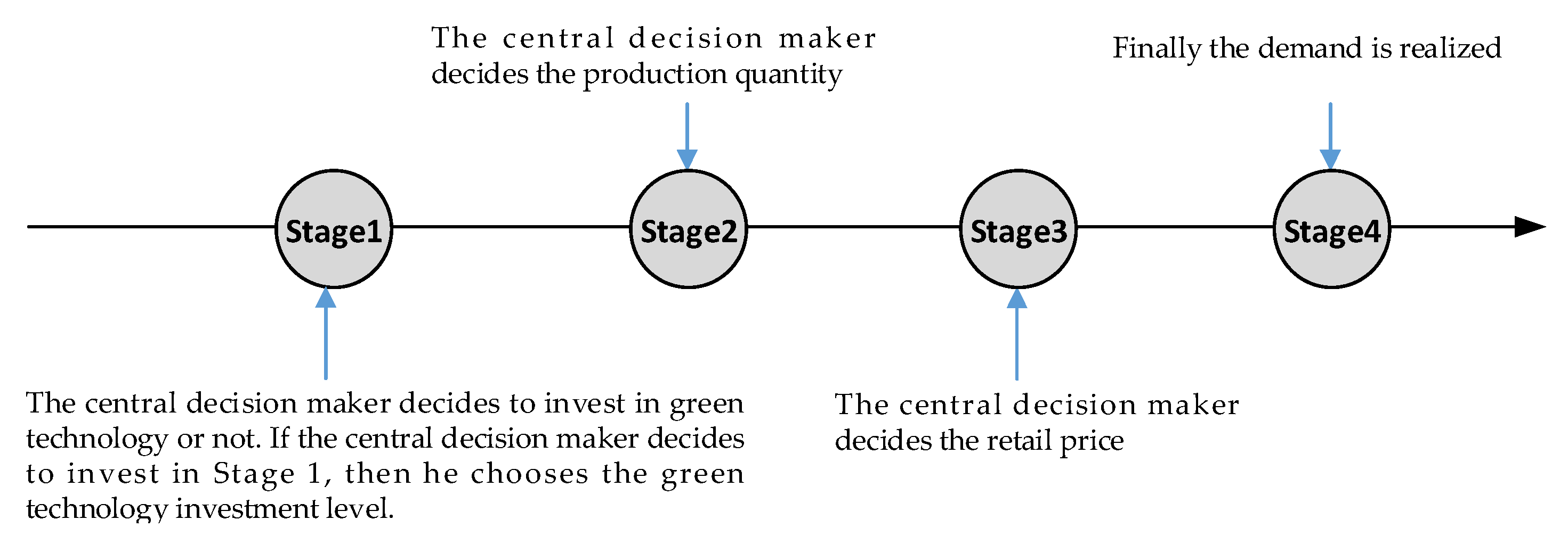
3.1. Scenario CI—The Centralized Supply Chain

There is a central decision-maker (he, denoted by CI) in Scenario CI who maximizes the whole supply chain’s expected profit as follows:

$$\underset{\mathrm{p},\mathrm{Q},\mathrm{s}}{\mathrm{m}\mathrm{a}\mathrm{x}}{\mathsf{\Pi }}_{\mathrm{C}\mathrm{I}}=\mathrm{E}[\mathrm{p}\mathrm{m}\mathrm{i}\mathrm{n}\left(\mathrm{D},\mathrm{Q}\right)-\mathrm{c}\mathrm{Q}]-\frac{\mathsf{\eta }}{2}{\left(1+\mathrm{s}\right)}^2.$$

(3)

Figure 1 illustrates the timing of the events. In stage 1, the central decision-maker decides to invest in green technology or not, and chooses the level $\mathrm{s}$ if he decides to invest. Then, he decides the production quantity $\mathrm{Q}$ in Stage 2. In Stage 3, he decides the retail price $\mathrm{p}$. Finally, the central decision-maker observes the realized demand in Stage 4.

We use backward induction to solve the decision problem. Following Wang et al. [61], we define the stocking factor of inventory as $\mathrm{z}=\mathrm{Q}/\mathrm{Y}\left(\mathrm{p},\mathrm{s}\right)$, where $\mathrm{Y}\left(\mathrm{p},\mathrm{s}\right)=\mathsf{\kappa }{\mathrm{p}}^{-\alpha }{\left(1+\mathrm{s}\right)}^{\lambda }$. Thus, the central supply chain’s decision problem can be rewritten as a decision problem of decision variables $\mathrm{s}$, $\mathrm{z}$, and $\mathrm{p}$ as follows:

$$\begin{array}{ll}\underset{\mathrm{p},\mathrm{z},\mathrm{s}}{\mathrm{m}\mathrm{a}\mathrm{x}}{\mathsf{\Pi }}_{\mathrm{C}\mathrm{I}}& =\mathsf{\kappa }{\mathrm{p}}^{-\alpha }{\left(1+\mathrm{s}\right)}^{\lambda }\mathrm{E}[\mathrm{p}\mathrm{m}\mathrm{i}\mathrm{n}\left(\mathsf{\epsilon },\mathrm{z}\right)-\mathrm{c}\mathrm{z}]-\frac{\mathsf{\eta }}{2}{\left(1+\mathrm{s}\right)}^2\\ & =\mathsf{\kappa }{\mathrm{p}}^{-\alpha }{\left(1+\mathrm{s}\right)}^{\lambda }\left[\mathrm{p}\left(\mathrm{z}-\mathsf{\Lambda }\left(\mathrm{z}\right)\right)-\mathrm{c}\mathrm{z}\right]-\frac{\mathsf{\eta }}{2}{\left(1+\mathrm{s}\right)}^2,\end{array}$$

(4)

where $\mathsf{\Lambda }\left(\mathrm{z}\right)={\int }_0^{\mathrm{z}}\left(\mathrm{z}-\mathrm{x}\right)\mathrm{f}\left(\mathrm{x}\right)\mathrm{d}\mathrm{x}$.

In Stage 3, differentiating ${\mathsf{\Pi }}_{\mathrm{C}\mathrm{I}}$ with respect to the retail price $\mathrm{p}$, we can obtain the optimal retail price for the given stocking factor $\mathrm{z}$ as follows.

For the given stocking factor $\mathrm{z}$ and green technology investment level $\mathrm{s}$, the optimal response of retail price $\mathrm{p}$ in the CI is as follows:

$$\mathrm{p}\left(\mathrm{z}\right)=\frac{\alpha \mathrm{c}\mathrm{z}}{\left(\alpha -1\right)\left(\mathrm{z}-\mathsf{\Lambda }\left(\mathrm{z}\right)\right)}.$$

(5)

All proofs are given in Appendix A.

The optimal response of retail price $\mathrm{p}\left(\mathrm{z}\right)$ is affected by the stocking factor $\mathrm{z}$ and production cost $\mathrm{c}$. Defining $\mathrm{m}\left(\alpha \right)=\alpha /\left(\alpha -1\right)$ and $\mathrm{n}\left(\mathrm{z}\right)=\mathrm{z}/\left(\mathrm{z}-\mathsf{\Lambda }\left(\mathrm{z}\right)\right)$, we find $\partial \mathrm{m}\left(\alpha \right)/\partial \alpha ={-1/\left(\alpha -1\right)}^2<0$ and $\partial \mathrm{n}\left(\mathrm{z}\right)/\partial \mathrm{z}={\int }_0^{\mathrm{z}}xf\left(x\right)dx/{\left(\mathrm{z}-\mathsf{\Lambda }\left(\mathrm{z}\right)\right)}^2>0$. Therefore, when the price elasticity is larger, the retail price is more sensitive to the production cost. On the contrary, when the stocking factor is larger, the retail price is less sensitive to the production cost. However, the optimal response of retail price $\mathrm{p}\left(\mathrm{z}\right)$ is independent of the green technology investment level $\mathrm{s}$.

Next, we solve the optimal response stocking factor $\mathrm{z}$. To derive the closed-form solutions, following Wang et al. [61], and Wang [64], we assume the demand stochastic $\mathsf{\epsilon }$ is uniformly distributed on $[0,2\mathsf{\mu }]$ later in the paper. Then, we can get $\mathsf{\Lambda }\left(\mathrm{z}\right)=\frac{{\mathrm{z}}^2}{4\mathsf{\mu }}$.

Thus, in Stage 2, the central supply chain’s decision problem can be rewritten as a decision problem of decision variable $\mathrm{z}$ as follows:

$$\underset{\mathrm{z}}{\mathrm{m}\mathrm{a}\mathrm{x}}{\mathsf{\Pi }}_{\mathrm{C}\mathrm{I}}=\frac{\mathsf{\kappa }{\left(1+\mathrm{s}\right)}^{\lambda }{\left(\alpha -1\right)}^{\alpha -1}{\left(4\mathsf{\mu }-\mathrm{z}\right)}^{\alpha }\mathrm{z}}{4^{\alpha }{\mathsf{\mu }}^{\alpha }{\alpha }^{\alpha }{\mathrm{c}}^{\alpha -1}}-\frac{\mathsf{\eta }}{2}{\left(1+\mathrm{s}\right)}^2.$$

(6)

From the first condition, we derive the optimal stocking factor as follows:

$${\mathrm{z}}_{\mathrm{C}\mathrm{I}}^{*}=\frac{4\mathsf{\mu }}{1+\alpha }.$$

(7)

Last, in Stage 1, we solve the green technology investment level $\mathrm{s}$. Substituting ${\mathrm{z}}_{\mathrm{C}\mathrm{I}}^{*}$ into (6), we derive the decision problem of the green technology investment level $\mathrm{s}$ as follows:

$$\underset{\mathrm{s}}{\mathrm{m}\mathrm{a}\mathrm{x}}{\mathsf{\Pi }}_{\mathrm{C}\mathrm{I}}=\frac{4\mathsf{\mu }\mathsf{\kappa }{\left(1+\mathrm{s}\right)}^{\lambda }{\left(\alpha -1\right)}^{\alpha -1}}{{\mathrm{c}}^{\alpha -1}{\left(1+\alpha \right)}^{1+\alpha }}-\frac{\mathsf{\eta }}{2}{\left(1+\mathrm{s}\right)}^2.$$

(8)

From the first condition, we derive the optimal green technology investment level as follows:

$${\mathrm{s}}_{\mathrm{C}\mathrm{I}}^{*}=\mathrm{m}\mathrm{a}\mathrm{x}\left\{\sqrt[2-\lambda ]{\frac{4\lambda \mathsf{\mu }\mathsf{\kappa }{\left(\alpha -1\right)}^{\alpha -1}}{\mathsf{\eta }{\mathrm{c}}^{\alpha -1}{\left(1+\alpha \right)}^{1+\alpha }}}-1,0\right\}.$$

(9)

In fact, when the central decision-maker does not invest in green technology, the central supply chain’s expected profit is as follows:

$${\mathsf{\Pi }}_{\mathrm{C}\mathrm{I}-N}^{*}=\frac{4\mathsf{\mu }\mathsf{\kappa }{\left(\alpha -1\right)}^{\alpha -1}}{{\mathrm{c}}^{\alpha -1}{\left(1+\alpha \right)}^{1+\alpha }}.$$

(10)

And when he invests in green technology, then ${\mathrm{s}}_{\mathrm{C}\mathrm{I}}^{*}=\sqrt[2-\lambda ]{\frac{4\lambda \mathsf{\mu }\mathsf{\kappa }{\left(\alpha -1\right)}^{\alpha -1}}{\mathsf{\eta }{\mathrm{c}}^{\alpha -1}{\left(1+\alpha \right)}^{1+\alpha }}}-1$ and the central supply chain’s expected profit is as follows:

$${\mathsf{\Pi }}_{\mathrm{C}\mathrm{I}}^{*}=\frac{2\left(2-\lambda \right)\mathsf{\mu }\mathsf{\kappa }{\left(1+{\mathrm{s}}_{\mathrm{C}\mathrm{I}}^{*}\right)}^{\lambda }{\left(\alpha -1\right)}^{\alpha -1}}{{\mathrm{c}}^{\alpha -1}{\left(1+\alpha \right)}^{1+\alpha }}.$$

(11)

Substituting ${\mathrm{s}}_{\mathrm{C}\mathrm{I}}^{*}$ and ${\mathrm{z}}_{\mathrm{C}\mathrm{I}}^{*}$ into the retail price, production quantity, leftovers, and expected profit of the central supply chain, we can get the equilibrium decision variables and expected equilibrium profits of the supply-chain members in Scenario CI, as Proposition 1 presents.

Proposition 1. 

The decision variables and expected equilibrium profits of the supply-chain members in Scenario CI are summarized in

Table 2. The equilibrium results in model CI.

Scenario CI
${\mathrm{p}}_{\mathrm{C}\mathrm{I}}^{*}=\frac{\left(1+\alpha \right)\mathrm{c}}{\alpha -1}$	${\mathrm{Q}}_{\mathrm{C}\mathrm{I}}^{*}=\frac{4\mathsf{\mu }\mathsf{\kappa }{\left(\alpha -1\right)}^{\alpha }}{{\left(1+\alpha \right)}^{1+\alpha }{\mathrm{c}}^{\alpha }}{\left(\frac{4\lambda \mathsf{\mu }\mathsf{\kappa }{\left(\alpha -1\right)}^{\alpha -1}}{\mathsf{\eta }{\mathrm{c}}^{\alpha -1}{\left(1+\alpha \right)}^{1+\alpha }}\right)}^{\frac{\lambda }{2-\lambda }}$
${\mathrm{s}}_{\mathrm{C}\mathrm{I}}^{*}=\mathrm{m}\mathrm{a}\mathrm{x}\left\{\sqrt[2-\lambda ]{\frac{4\lambda \mathsf{\mu }\mathsf{\kappa }{\left(\alpha -1\right)}^{\alpha -1}}{\mathsf{\eta }{\mathrm{c}}^{\alpha -1}{\left(1+\alpha \right)}^{1+\alpha }}}-1,0\right\}$	$\mathrm{V}{\mathrm{Q}}_{\mathrm{C}\mathrm{I}}^{*}=\mathrm{m}\mathrm{a}\mathrm{x}\left\{\frac{\mathsf{\kappa }\left(3-\alpha \right)\mathsf{\mu }{\left(\alpha -1\right)}^{\alpha }}{{\left(1+\alpha \right)}^{\alpha +1}{\mathrm{c}}^{\alpha }}{\left(\frac{4\lambda \mathsf{\mu }\mathsf{\kappa }{\left(\alpha -1\right)}^{\alpha -1}}{\mathsf{\eta }{\mathrm{c}}^{\alpha -1}{\left(1+\alpha \right)}^{1+\alpha }}\right)}^{\frac{\lambda }{2-\lambda }},0\right\}$
${\mathsf{\Pi }}_{\mathrm{C}\mathrm{I}-\mathrm{N}}^{*}=\frac{4\mathsf{\mu }\mathsf{\kappa }{\left(\alpha -1\right)}^{\alpha -1}}{{\mathrm{c}}^{\alpha -1}{\left(1+\alpha \right)}^{1+\alpha }}$	${\mathsf{\Pi }}_{\mathrm{C}\mathrm{I}}^{*}=\frac{2\left(2-\lambda \right)\mathsf{\mu }\mathsf{\kappa }{\left(\alpha -1\right)}^{\alpha -1}{\left(4\lambda \mathsf{\mu }\mathsf{\kappa }{\left(\alpha -1\right)}^{\alpha -1}\right)}^{\frac{\lambda }{2-\lambda }}}{{\mathrm{c}}^{\alpha -1}{\left(1+\alpha \right)}^{1+\alpha }{\left(\mathsf{\eta }{\mathrm{c}}^{\alpha -1}{\left(1+\alpha \right)}^{1+\alpha }\right)}^{\frac{\lambda }{2-\lambda }}}$

.

Corollary 1. 

In Scenario CI, there is a threshold value${\mathsf{\eta }}_{\mathrm{C}\mathrm{I}}$, when the green technology investment coefficient meets$\mathsf{\eta }<{\mathsf{\eta }}_{\mathrm{C}\mathrm{I}}$,and the central decision-maker will invest in green technology, otherwise, he will not invest, where${\mathsf{\eta }}_{\mathrm{C}\mathrm{I}}$is as follows:

$${\mathsf{\eta }}_{\mathrm{C}\mathrm{I}}=\frac{4\lambda \mathsf{\mu }\mathsf{\kappa }{\left(\alpha -1\right)}^{\alpha -1}}{{\mathrm{c}}^{\alpha -1}{\left(1+\alpha \right)}^{1+\alpha }}{\left(\frac{2-\lambda }{2}\right)}^{\frac{2-\lambda }{\lambda }}.$$

(12)

Corollary 1 shows that whether the central decision-maker invests in green technology or not depends critically on the green technology investment coefficient $\mathsf{\eta }$. When the green technology investment coefficient is relatively large ($\mathsf{\eta }\ge {\mathsf{\eta }}_{\mathrm{C}\mathrm{I}}$), the decision-maker does not invest in green technology; and if and only if the green technology investment coefficient is relatively small ($\mathsf{\eta }<{\mathsf{\eta }}_{\mathrm{C}\mathrm{I}}$), he will invest in green technology. This result is intuitive. A low value $\mathsf{\eta }$ means a relatively low investment cost, which encourages the decision-maker to invest in green technology.

Next, we consider the following two scenarios: the supplier invests in green technology (Scenario SI) and the retailer invests in green technology (Scenario RI).

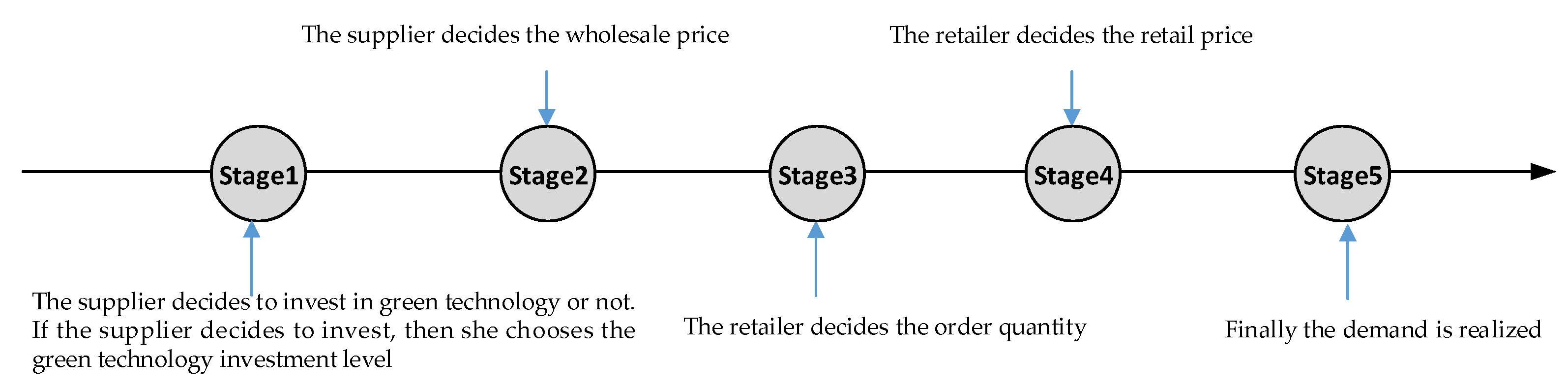
3.2. Scenario SI—The Supplier Investing in Green Technology

In Scenario SI, the supplier invests in green technology. Figure 2 illustrates the timing of the events. In Stage 1, the supplier decides to invest in green technology or not. If she decides to invest, then she chooses the green technology investment level $\mathrm{s}$. Then, in Stage 2, the supplier announces the wholesale price $\mathrm{w}$. After observing the wholesale price $\mathrm{w}$, the retailer decides the order quantity $\mathrm{Q}$ in Stage 3. In Stage 4, the retailer decides the retail price $\mathrm{p}$. Finally, the demand is realized.

The decision problem of the supplier and retailer can be written as a decision problem of decision variables $\mathrm{s}$, $\mathrm{w}$, $\mathrm{z}$, and $\mathrm{p}$ as follows:

$$\underset{\mathrm{s},\mathrm{w}}{\mathrm{m}\mathrm{a}\mathrm{x}}{\mathsf{\Pi }}_{\mathrm{S}\mathrm{I}}^{\mathrm{S}}=\left(\mathrm{w}-\mathrm{c}\right)\mathrm{Q}-\frac{\mathsf{\eta }}{2}{\left(1+\mathrm{s}\right)}^2,$$

(13)

$$\begin{array}{ll}\underset{\mathrm{p},\mathrm{z}}{\mathrm{m}\mathrm{a}\mathrm{x}}{\mathsf{\Pi }}_{\mathrm{S}\mathrm{I}}^{\mathrm{R}}& =\mathrm{E}[\mathrm{p}\mathrm{m}\mathrm{i}\mathrm{n}\left(\mathrm{D},\mathrm{Q}\right)-\mathrm{w}\mathrm{Q}]\\ & =\mathsf{\kappa }{\mathrm{p}}^{-\alpha }{\left(1+\mathrm{s}\right)}^{\lambda }\left[\mathrm{p}\left(\mathrm{z}-\mathsf{\Lambda }\left(\mathrm{z}\right)\right)-\mathrm{w}\mathrm{z}\right].\end{array}$$

(14)

Similar to Scenario CI, we use backward induction to solve the multistage game. We first solve the retailer’s decision problem of decision variable $\mathrm{p}$ as follows:

$$\begin{array}{ll}\underset{\mathrm{p}}{\mathrm{m}\mathrm{a}\mathrm{x}}{\mathsf{\Pi }}_{\mathrm{S}\mathrm{I}}^{\mathrm{R}}& =\mathrm{E}[\mathrm{p}\mathrm{m}\mathrm{i}\mathrm{n}\left(\mathrm{D},\mathrm{Q}\right)-\mathrm{w}\mathrm{Q}]\\ & =\mathsf{\kappa }{\mathrm{p}}^{-\alpha }{\left(1+\mathrm{s}\right)}^{\lambda }\left[\mathrm{p}\left(\mathrm{z}-\mathsf{\Lambda }\left(\mathrm{z}\right)\right)-\mathrm{w}\mathrm{z}\right].\end{array}$$

(15)

Differentiating ${\mathsf{\Pi }}_{\mathrm{S}\mathrm{I}}^{\mathrm{R}}$ with respect to $\mathrm{p}$, we can obtain the optimal retail price for the given stocking factor $\mathrm{z}$, and green technology investment level $\mathrm{s}$.

For the given stocking factor $\mathrm{z}$ and green technology investment level $\mathrm{s}$, the optimal response of retail price $\mathrm{p}$ in the supply chain when the supplier invests in green technology is as follows:

$$\mathrm{p}=\frac{\alpha \mathrm{z}\mathrm{w}}{\left(\alpha -1\right)\left(\mathrm{z}-\mathsf{\Lambda }\left(\mathrm{z}\right)\right)}.$$

(16)

Then, substituting (16) into the retailer’s objective, we obtain the decision problem in Stage 4 as follows:

$$\underset{\mathrm{z}}{\mathrm{m}\mathrm{a}\mathrm{x}}{\mathsf{\Pi }}_{\mathrm{S}\mathrm{I}}^{\mathrm{R}}=\frac{\mathsf{\kappa }{\left(\alpha -1\right)}^{\alpha -1}{\left(\mathrm{z}-\mathsf{\Lambda }\left(\mathrm{z}\right)\right)}^{\alpha }{\left(1+\mathrm{s}\right)}^{\lambda }}{{\alpha }^{\alpha }{\mathrm{w}}^{\alpha -1}{\mathrm{z}}^{\alpha -1}}.$$

(17)

Because the $\mathsf{\epsilon }\in \mathrm{U}[0,2\mathsf{\mu }]$ from the first condition of ${\mathsf{\Pi }}_{\mathrm{S}\mathrm{I}}^{\mathrm{R}}$, we derive the optimal stocking factor as follows:

$${\mathrm{z}}_{\mathrm{S}\mathrm{I}}^{*}=\frac{4\mathsf{\mu }}{1+\alpha }.$$

(18)

Substituting (18) into (16), we have

$${\mathrm{p}}_{\mathrm{S}\mathrm{I}}^{*}=\frac{\left(1+\alpha \right)\mathrm{w}}{\alpha -1}.$$

(19)

In Stage 2, the supplier decides the wholesale price $\mathrm{w}$. Substituting (18) and (19) into the supplier’s decision problem, we have

$$\underset{\mathrm{w}}{\mathrm{m}\mathrm{a}\mathrm{x}}{\mathsf{\Pi }}_{\mathrm{S}\mathrm{I}}^{\mathrm{S}}=\frac{4\mathsf{\mu }\mathsf{\kappa }{\left(1+\mathrm{s}\right)}^{\lambda }{\left(\alpha -1\right)}^{\alpha }\left(\mathrm{w}-\mathrm{c}\right)}{{\left(1+\alpha \right)}^{\alpha +1}{\mathrm{w}}^{\alpha }}-\frac{\mathsf{\eta }}{2}{\left(1+\mathrm{s}\right)}^2.$$

(20)

From the first condition, we derive the optimal wholesale price as follows:

$${\mathrm{w}}_{\mathrm{S}\mathrm{I}}^{*}=\frac{\alpha \mathrm{c}}{\alpha -1}.$$

(21)

Last, in Stage 1, the supplier decides the green technology investment level $\mathrm{s}$. Substituting ${\mathrm{z}}_{\mathrm{S}\mathrm{I}}^{*}$ into (20), we derive the decision problem of the green technology investment level $\mathrm{s}$ as follows:

$$\underset{\mathrm{s}}{\mathrm{m}\mathrm{a}\mathrm{x}}{\mathsf{\Pi }}_{\mathrm{S}\mathrm{I}}^{\mathrm{S}}=\frac{4\mathsf{\mu }\mathsf{\kappa }{\left(\alpha -1\right)}^{2\alpha -1}{\left(1+\mathrm{s}\right)}^{\lambda }}{{\left(1+\alpha \right)}^{\alpha +1}{\alpha }^{\alpha }{\mathrm{c}}^{\alpha -1}}-\frac{\mathsf{\eta }}{2}{\left(1+\mathrm{s}\right)}^2.$$

(22)

From the first condition, the optimal green technology investment level is obtained as follows:

$${\mathrm{s}}_{\mathrm{S}\mathrm{I}}^{*}=\mathrm{m}\mathrm{a}\mathrm{x}\left\{\sqrt[2-\lambda ]{\frac{4\lambda \mathsf{\mu }\mathsf{\kappa }{\left(\alpha -1\right)}^{2\alpha -1}}{\mathsf{\eta }{\left(1+\alpha \right)}^{\alpha +1}{\alpha }^{\alpha }{\mathrm{c}}^{\alpha -1}}}-1,0\right\}.$$

(23)

The supplier’s expected profit is as follows:

$${\mathsf{\Pi }}_{\mathrm{S}\mathrm{I}}^{\mathrm{S}*}=\frac{2\left(2-\lambda \right)\mathsf{\kappa }\mathsf{\mu }{\left(1+{\mathrm{s}}_{\mathrm{S}\mathrm{I}}^{*}\right)}^{\lambda }{\left(\alpha -1\right)}^{2\alpha -1}}{{\left(1+\alpha \right)}^{\alpha +1}{\alpha }^{\alpha }{\mathrm{c}}^{\alpha -1}}.$$

(24)

When the supplier does not invest in green technology, the supplier’s expected profit is given as follows:

$${\mathsf{\Pi }}_{\mathrm{S}\mathrm{I}-\mathrm{N}}^{\mathrm{S}*}=\frac{4\mathsf{\mu }\mathsf{\kappa }{\left(\alpha -1\right)}^{2\alpha -1}}{{\left(1+\alpha \right)}^{\alpha +1}{\alpha }^{\alpha }{\mathrm{c}}^{\alpha -1}}.$$

(25)

Substituting ${\mathrm{s}}_{\mathrm{S}\mathrm{I}}^{*}$ and ${\mathrm{z}}_{\mathrm{S}\mathrm{I}}^{*}$ into the retail price, production quantity, leftovers, and expected profit of the supply-chain members, we can get the equilibrium decision variables and expected equilibrium profits of the supply-chain members in Scenario SI, as Proposition 2 presents.

Proposition 2. 

The decision variables and expected equilibrium profits of the supply-chain members in Scenario SI are summarized in

Table 3. The equilibrium results in model SI.

Scenario SI
${\mathrm{p}}_{\mathrm{S}\mathrm{I}}^{*}=\frac{\alpha \mathrm{c}\left(1+\alpha \right)}{{\left(\alpha -1\right)}^2}$	${\mathrm{Q}}_{\mathrm{S}\mathrm{I}}^{*}=\frac{4\mathsf{\mu }\mathsf{\kappa }{\left(\alpha -1\right)}^{2\alpha }}{{\alpha }^{\alpha }{\mathrm{c}}^{\alpha }{\left(1+\alpha \right)}^{\alpha +1}}{\left(\frac{4\lambda \mathsf{\mu }\mathsf{\kappa }{\left(\alpha -1\right)}^{2\alpha -1}}{\mathsf{\eta }{\left(1+\alpha \right)}^{\alpha +1}{\alpha }^{\alpha }{\mathrm{c}}^{\alpha -1}}\right)}^{\frac{\lambda }{2-\lambda }}$
${\mathrm{w}}_{\mathrm{S}\mathrm{I}}^{*}=\frac{\alpha \mathrm{c}}{\alpha -1}$	$\mathrm{V}{\mathrm{Q}}_{\mathrm{S}\mathrm{I}}^{*}=\mathrm{m}\mathrm{a}\mathrm{x}\left\{\frac{\mathsf{\kappa }\left(3-\alpha \right)\mathsf{\mu }{\left(\alpha -1\right)}^{2\alpha }}{{\alpha }^{\alpha }{\mathrm{c}}^{\alpha }{\left(1+\alpha \right)}^{\alpha +1}}{\left(\frac{4\lambda \mathsf{\mu }\mathsf{\kappa }{\left(\alpha -1\right)}^{2\alpha -1}}{\mathsf{\eta }{\left(1+\alpha \right)}^{\alpha +1}{\alpha }^{\alpha }{\mathrm{c}}^{\alpha -1}}\right)}^{\frac{\lambda }{2-\lambda }},0\right\}$
${\mathrm{s}}_{\mathrm{S}\mathrm{I}}^{*}=\mathrm{m}\mathrm{a}\mathrm{x}\left\{\sqrt[2-\lambda ]{\frac{4\lambda \mathsf{\mu }\mathsf{\kappa }{\left(\alpha -1\right)}^{2\alpha -1}}{\mathsf{\eta }{\left(1+\alpha \right)}^{\alpha +1}{\alpha }^{\alpha }{\mathrm{c}}^{\alpha -1}}}-1,0\right\}$
${\mathsf{\Pi }}_{\mathrm{S}\mathrm{I}-\mathrm{N}}^{\mathrm{S}*}=\frac{4\mathsf{\mu }\mathsf{\kappa }{\left(\alpha -1\right)}^{2\alpha -1}}{{\left(1+\alpha \right)}^{\alpha +1}{\alpha }^{\alpha }{\mathrm{c}}^{\alpha -1}}$	${\mathsf{\Pi }}_{\mathrm{S}\mathrm{I}}^{\mathrm{S}*}=\frac{2\left(2-\lambda \right)\mathsf{\kappa }\mathsf{\mu }{\left(\alpha -1\right)}^{2\alpha -1}{\left(4\lambda \mathsf{\mu }\mathsf{\kappa }{\left(\alpha -1\right)}^{2\alpha -1}\right)}^{\frac{\lambda }{2-\lambda }}}{{\left(1+\alpha \right)}^{\alpha +1}{\alpha }^{\alpha }{\mathrm{c}}^{\alpha -1}{\left(\mathsf{\eta }{\left(1+\alpha \right)}^{\alpha +1}{\alpha }^{\alpha }{\mathrm{c}}^{\alpha -1}\right)}^{\frac{\lambda }{2-\lambda }}}$
${\mathsf{\Pi }}_{\mathrm{S}\mathrm{I}-\mathrm{N}}^{\mathrm{R}*}=\frac{4\mathsf{\mu }\mathsf{\kappa }{\left(\alpha -1\right)}^{2\alpha -2}}{{\alpha }^{\alpha -1}{\left(1+\alpha \right)}^{\alpha +1}{\mathrm{c}}^{\alpha -1}}$	${\mathsf{\Pi }}_{\mathrm{S}\mathrm{I}}^{\mathrm{R}*}=\frac{4\mathsf{\mu }\mathsf{\kappa }{\left(\alpha -1\right)}^{2\alpha -2}{\left(4\lambda \mathsf{\mu }\mathsf{\kappa }{\left(\alpha -1\right)}^{2\alpha -1}\right)}^{\frac{\lambda }{2-\lambda }}}{{\alpha }^{\alpha -1}{\left(1+\alpha \right)}^{\alpha +1}{\mathrm{c}}^{\alpha -1}{\left(\mathsf{\eta }{\left(1+\alpha \right)}^{\alpha +1}{\alpha }^{\alpha }{\mathrm{c}}^{\alpha -1}\right)}^{\frac{\lambda }{2-\lambda }}}$

.

Corollary 2. 

In Scenario SI,there is a threshold value${\mathsf{\eta }}_{\mathrm{S}\mathrm{I}}$, when the green technology investment coefficient meets$\mathsf{\eta }<{\mathsf{\eta }}_{\mathrm{S}\mathrm{I}}$, and the supplier will invest in green technology, otherwise, she will not invest, where${\mathsf{\eta }}_{\mathrm{S}\mathrm{I}}$is as follows:

$${\mathsf{\eta }}_{\mathrm{S}\mathrm{I}}=\frac{4\lambda \mathsf{\mu }\mathsf{\kappa }{\left(\alpha -1\right)}^{2\alpha -1}}{{\left(1+\alpha \right)}^{\alpha +1}{\alpha }^{\alpha }{\mathrm{c}}^{\alpha -1}}{\left(\frac{2-\lambda }{2}\right)}^{\frac{2-\lambda }{\lambda }}.$$

(26)

Corollary 2 obtains the threshold of the green technology investment coefficient that the supplier can afford. When the green technology investment coefficient is relatively large to the supplier ($\mathsf{\eta }\ge {\mathsf{\eta }}_{\mathrm{S}\mathrm{I}}$), she does not invest in green technology; and if and only if the green technology investment coefficient is relatively small ($\mathsf{\eta }<{\mathsf{\eta }}_{\mathrm{S}\mathrm{I}}$), she will invest in green technology.

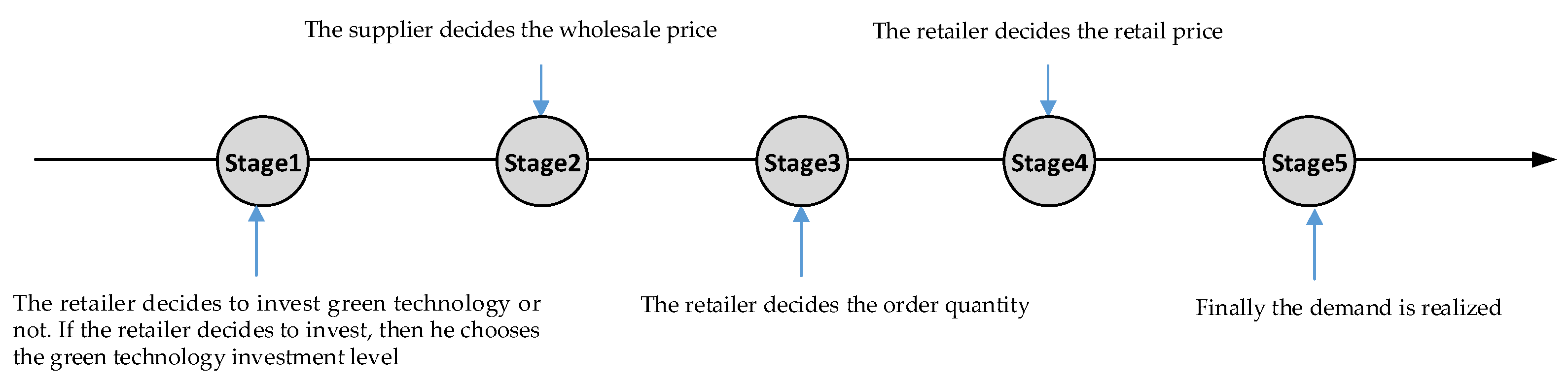
3.3. Scenario RI—The Retailer Investing in Green Technology

The only difference between Scenarios SI and RI is that the retailer invests in green technology. So, in Stage 1, the retailer decides to invest in green technology or not, and he chooses the green technology investment level $\mathrm{s}$ if he decides to invest. Other stages are the same as the stages in Scenario SI, and Figure 3 illustrates the timing of the events.

The decision problem in this scenario of the supplier and retailer can be written as a decision problem of decision variables $\mathrm{s}$, $\mathrm{w}$, $\mathrm{z}$, and $\mathrm{p}$ as follows:

$$\underset{\mathrm{w}}{\mathrm{m}\mathrm{a}\mathrm{x}}{\mathsf{\Pi }}_{\mathrm{R}\mathrm{I}}^{\mathrm{S}}=\left(\mathrm{w}-\mathrm{c}\right)\mathrm{Q},$$

(27)

$$\begin{array}{ll}\underset{\mathrm{s},\mathrm{p},\mathrm{z}}{\mathrm{m}\mathrm{a}\mathrm{x}}{\mathsf{\Pi }}_{\mathrm{R}\mathrm{I}}^{\mathrm{R}}& =\mathrm{E}[\mathrm{p}\mathrm{m}\mathrm{i}\mathrm{n}\left(\mathrm{D},\mathrm{Q}\right)-\mathrm{w}\mathrm{Q}-\frac{\mathsf{\eta }}{2}{\left(1+\mathrm{s}\right)}^2]\\ & =\mathsf{\kappa }{\mathrm{p}}^{-\alpha }{\left(1+\mathrm{s}\right)}^{\lambda }\left[\mathrm{p}\left(\mathrm{z}-\mathsf{\Lambda }\left(\mathrm{z}\right)\right)-\mathrm{w}\mathrm{z}-\frac{\mathsf{\eta }}{2}{\left(1+\mathrm{s}\right)}^2\right].\end{array}$$

(28)

We use backward induction to solve the multistage game in Scenario RI. Because the solving process of Stages 2–4 in Scenario RI is the same as the process in Scenario SI, we omit it. We only focus on the decision problem in Stage 1—the retailer decides the green technology investment level $\mathrm{s}$. Substituting the results obtained in Stages 2–4 into the retailer’s objective function, we can write the retailer’ decision problem of the green technology investment level $\mathrm{s}$ as follows:

$$\underset{\mathrm{s}}{\mathrm{m}\mathrm{a}\mathrm{x}}{\mathsf{\Pi }}_{\mathrm{R}\mathrm{I}}^{\mathrm{R}}=\frac{4\mathsf{\mu }\mathsf{\kappa }{\left(1+\mathrm{s}\right)}^{\lambda }{\left(\alpha -1\right)}^{2\alpha -2}}{{\alpha }^{\alpha -1}{\mathrm{c}}^{\alpha -1}{\left(1+\alpha \right)}^{1+\alpha }}-\frac{\mathsf{\eta }}{2}{\left(1+\mathrm{s}\right)}^2.$$

(29)

From the first condition, the optimal green technology investment level is obtained as follows:

$${\mathrm{s}}_{\mathrm{R}\mathrm{I}}^{*}=\mathrm{m}\mathrm{a}\mathrm{x}\left\{\sqrt[2-\lambda ]{\frac{4\lambda \mathsf{\mu }\mathsf{\kappa }{\left(\alpha -1\right)}^{2\alpha -2}}{\mathsf{\eta }{\alpha }^{\alpha -1}{\mathrm{c}}^{\alpha -1}{\left(1+\alpha \right)}^{1+\alpha }}}-1,0\right\}.$$

(30)

The retailer’s expected profit is as follows:

$${\mathsf{\Pi }}_{\mathrm{R}\mathrm{I}}^{\mathrm{R}*}=\frac{2\left(2-\lambda \right){\left(1+{\mathrm{s}}_{\mathrm{R}\mathrm{I}}^{*}\right)}^{\lambda }\mathsf{\mu }\mathsf{\kappa }{\left(\alpha -1\right)}^{2\alpha -2}}{{\alpha }^{\alpha -1}{\mathrm{c}}^{\alpha -1}{\left(1+\alpha \right)}^{1+\alpha }}.$$

(31)

When the retailer does not invest in green technology, the retailer’s expected profit is given as follows:

$${\mathsf{\Pi }}_{\mathrm{R}\mathrm{I}-\mathrm{N}}^{\mathrm{R}*}=\frac{4\mathsf{\mu }\mathsf{\kappa }{\left(\alpha -1\right)}^{2\alpha -2}}{{\alpha }^{\alpha -1}{\mathrm{c}}^{\alpha -1}{\left(1+\alpha \right)}^{1+\alpha }}.$$

(32)

Substituting ${\mathrm{s}}_{\mathrm{R}\mathrm{I}}^{*}$, ${\mathrm{z}}_{\mathrm{R}\mathrm{I}}^{*}$ into the retail price, production quantity, leftovers, and expected profit of the supply-chain members, we can get the equilibrium decision variables and expected equilibrium profits of the supply-chain members in Scenario RI, as Proposition 3 presents.

Proposition 3. 

The decision variables and expected equilibrium profits of the supply-chain members in Scenario RI are summarized in

Table 4. The equilibrium results in model RI.

Scenario RI
${\mathrm{p}}_{\mathrm{R}\mathrm{I}}^{*}=\frac{\alpha \mathrm{c}\left(1+\alpha \right)}{{\left(\alpha -1\right)}^2}$	${\mathrm{Q}}_{\mathrm{R}\mathrm{I}}^{*}=\frac{4\mathsf{\mu }\mathsf{\kappa }{\left(\alpha -1\right)}^{2\alpha -1}}{{\alpha }^{\alpha }{\mathrm{c}}^{\alpha }{\left(1+\alpha \right)}^{\alpha +1}}{\left(\frac{4\lambda \mathsf{\mu }\mathsf{\kappa }{\left(\alpha -1\right)}^{2\alpha -2}}{\mathsf{\eta }{\alpha }^{\alpha -1}{\mathrm{c}}^{\alpha -1}{\left(1+\alpha \right)}^{1+\alpha }}\right)}^{\frac{\lambda }{2-\lambda }}$
${\mathrm{w}}_{\mathrm{R}\mathrm{I}}^{*}=\frac{\alpha \mathrm{c}}{\alpha -1}$	$\mathrm{V}{\mathrm{Q}}_{\mathrm{R}\mathrm{I}}^{*}=\mathrm{m}\mathrm{a}\mathrm{x}\left\{\frac{\mathsf{\kappa }\left(3-\alpha \right)\mathsf{\mu }{\left(\alpha -1\right)}^{2\alpha -1}}{{\alpha }^{\alpha }{\mathrm{c}}^{\alpha }{\left(1+\alpha \right)}^{\alpha +1}}{\left(\frac{4\lambda \mathsf{\mu }\mathsf{\kappa }{\left(\alpha -1\right)}^{2\alpha -2}}{\mathsf{\eta }{\alpha }^{\alpha -1}{\mathrm{c}}^{\alpha -1}{\left(1+\alpha \right)}^{1+\alpha }}\right)}^{\frac{\lambda }{2-\lambda }},0\right\}$
${\mathrm{s}}_{\mathrm{R}\mathrm{I}}^{*}=\mathrm{m}\mathrm{a}\mathrm{x}\left\{\sqrt[2-\lambda ]{\frac{4\lambda \mathsf{\mu }\mathsf{\kappa }{\left(\alpha -1\right)}^{2\alpha -2}}{\mathsf{\eta }{\alpha }^{\alpha -1}{\mathrm{c}}^{\alpha -1}{\left(1+\alpha \right)}^{1+\alpha }}}-1,0\right\}$
${\mathsf{\Pi }}_{\mathrm{R}\mathrm{I}-\mathrm{N}}^{\mathrm{S}*}=\frac{4\mathsf{\mu }\mathsf{\kappa }{\left(\alpha -1\right)}^{2\alpha -1}}{{\left(1+\alpha \right)}^{\alpha +1}{\alpha }^{\alpha }{\mathrm{c}}^{\alpha -1}}$	${\mathsf{\Pi }}_{\mathrm{R}\mathrm{I}}^{\mathrm{S}*}=\frac{4\mathsf{\mu }\mathsf{\kappa }{\left(\alpha -1\right)}^{2\alpha -1}{\left(4\lambda \mathsf{\mu }\mathsf{\kappa }{\left(\alpha -1\right)}^{2\alpha -2}\right)}^{\frac{\lambda }{2-\lambda }}}{{\left(1+\alpha \right)}^{\alpha +1}{\alpha }^{\alpha }{\mathrm{c}}^{\alpha -1}{\left(\mathsf{\eta }{\alpha }^{\alpha -1}{\mathrm{c}}^{\alpha -1}{\left(1+\alpha \right)}^{1+\alpha }\right)}^{\frac{\lambda }{2-\lambda }}}$
${\mathsf{\Pi }}_{\mathrm{R}\mathrm{I}-\mathrm{N}}^{\mathrm{R}*}=\frac{4\mathsf{\mu }\mathsf{\kappa }{\left(\alpha -1\right)}^{2\alpha -2}}{{\alpha }^{\alpha -1}{\mathrm{c}}^{\alpha -1}{\left(1+\alpha \right)}^{1+\alpha }}$	${\mathsf{\Pi }}_{\mathrm{R}\mathrm{I}}^{\mathrm{R}*}=\frac{2\left(2-\lambda \right)\mathsf{\mu }\mathsf{\kappa }{\left(\alpha -1\right)}^{2\alpha -2}{\left(4\lambda \mathsf{\mu }\mathsf{\kappa }{\left(\alpha -1\right)}^{2\alpha -2}\right)}^{\frac{\lambda }{2-\lambda }}}{{\alpha }^{\alpha -1}{\mathrm{c}}^{\alpha -1}{\left(1+\alpha \right)}^{1+\alpha }{\left(\mathsf{\eta }{\alpha }^{\alpha -1}{\mathrm{c}}^{\alpha -1}{\left(1+\alpha \right)}^{1+\alpha }\right)}^{\frac{\lambda }{2-\lambda }}}$

.

Corollary 3. 

In Scenario RI, there is a threshold value${\mathsf{\eta }}_{\mathrm{R}\mathrm{I}}$, when the green technology investment coefficient meets$\mathsf{\eta }<{\mathsf{\eta }}_{\mathrm{R}\mathrm{I}}$, and the retailer will invest in green technology, otherwise, he will not invest, where${\mathsf{\eta }}_{\mathrm{R}\mathrm{I}}$is as follows:

$${\mathsf{\eta }}_{\mathrm{R}\mathrm{I}}=\frac{4\lambda \mathsf{\mu }\mathsf{\kappa }{\left(\alpha -1\right)}^{2\alpha -2}}{{\alpha }^{\alpha -1}{\mathrm{c}}^{\alpha -1}{\left(1+\alpha \right)}^{1+\alpha }}{\left(\frac{2-\lambda }{2}\right)}^{\frac{2-\lambda }{\lambda }}.$$

(33)

Corollary 3 obtains the threshold of the green technology investment coefficient that the retailer can afford. When the green technology investment coefficient is relatively large to the retailer ($\mathsf{\eta }\ge {\mathsf{\eta }}_{\mathrm{R}\mathrm{I}}$), he does not invest in green technology; and if and only if the green technology investment coefficient is relatively small ($\mathsf{\eta }<{\mathsf{\eta }}_{\mathrm{R}\mathrm{I}}$), he will invest in green technology.

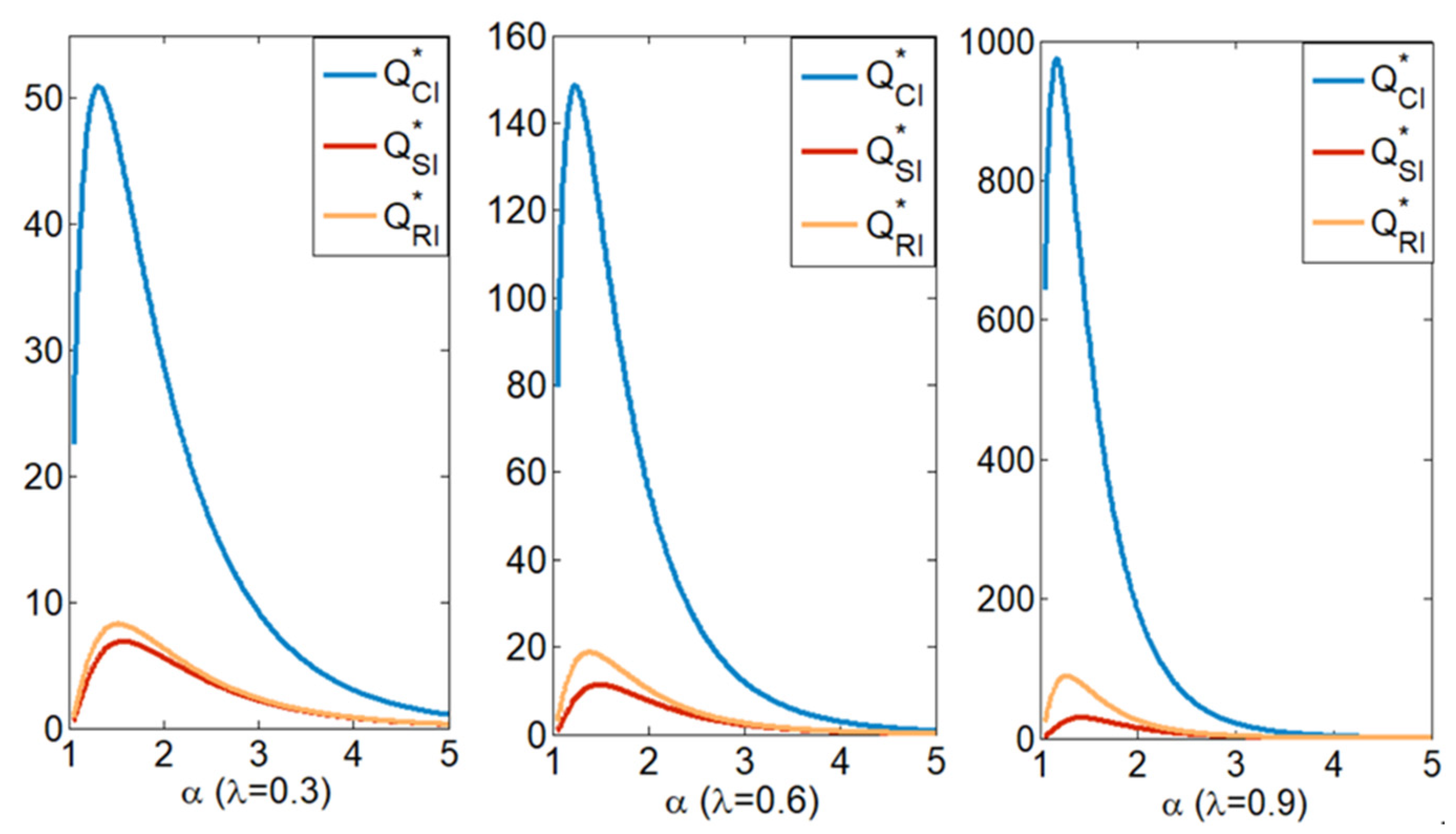
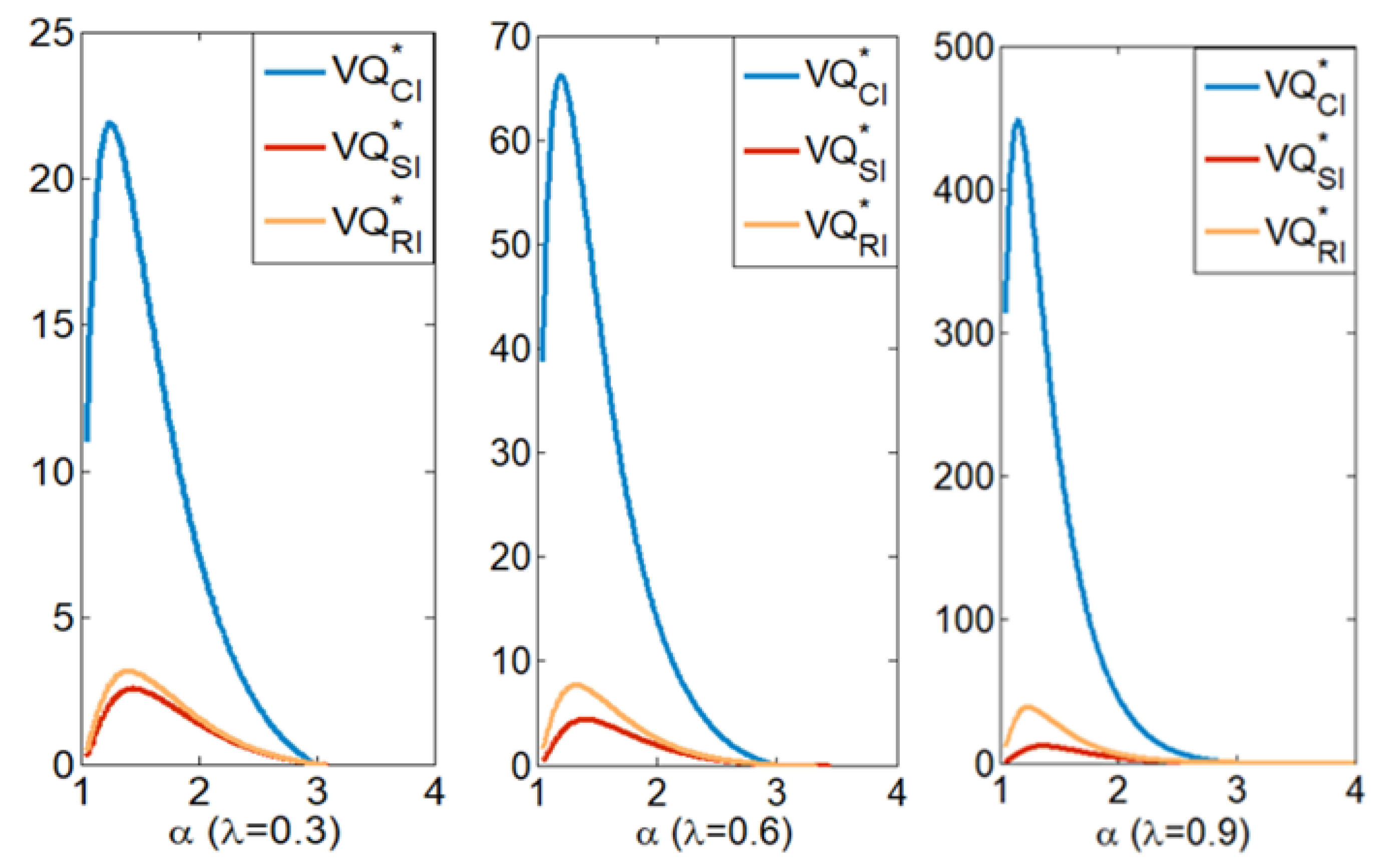
4. Operation Analysis

We compare and analyze the equilibrium results in different models and give the economic explanation in this operation analysis section. For easily comparing and analyzing the equilibrium results in different models, all the equilibrium results in different models in this paper are summarized and shown in

Table 5. The equilibrium results in different Scenarios.

	Scenario CI	Scenario SI	Scenario RI	Scenario CTSI
${\mathrm{p}}^{*}$	${\mathrm{p}}_{\mathrm{C}\mathrm{I}}^{*}=\frac{\left(1+\alpha \right)\mathrm{c}}{\alpha -1}$	${\mathrm{p}}_{\mathrm{S}\mathrm{I}}^{*}=\frac{\alpha \mathrm{c}\left(1+\alpha \right)}{{\left(\alpha -1\right)}^2}$	${\mathrm{p}}_{\mathrm{R}\mathrm{I}}^{*}=\frac{\alpha \mathrm{c}\left(1+\alpha \right)}{{\left(\alpha -1\right)}^2}$	${\mathrm{p}}_{\mathrm{C}\mathrm{T}\mathrm{S}\mathrm{I}}^{*}=\frac{\alpha \mathrm{c}\left(1+\alpha \right)}{{\left(\alpha -1\right)}^2}$
${\mathrm{w}}^{*}$	/	${\mathrm{w}}_{\mathrm{S}\mathrm{I}}^{*}=\frac{\alpha \mathrm{c}}{\alpha -1}$	${\mathrm{w}}_{\mathrm{R}\mathrm{I}}^{*}=\frac{\alpha \mathrm{c}}{\alpha -1}$	${\mathrm{w}}_{\mathrm{C}\mathrm{T}\mathrm{S}\mathrm{I}}^{*}=\frac{\alpha \mathrm{c}}{\alpha -1}$
${\mathrm{Q}}^{*}$	${\mathrm{Q}}_{\mathrm{C}\mathrm{I}}^{*}=\frac{4\mathsf{\mu }\mathsf{\kappa }{\left(\alpha -1\right)}^{\alpha }}{{\left(1+\alpha \right)}^{1+\alpha }{\mathrm{c}}^{\alpha }}{\left(\frac{4\lambda \mathsf{\mu }\mathsf{\kappa }{\left(\alpha -1\right)}^{\alpha -1}}{\mathsf{\eta }{\mathrm{c}}^{\alpha -1}{\left(1+\alpha \right)}^{1+\alpha }}\right)}^{\frac{\lambda }{2-\lambda }}$	${\mathrm{Q}}_{\mathrm{S}\mathrm{I}}^{*}=\frac{4\mathsf{\mu }\mathsf{\kappa }{\left(\alpha -1\right)}^{2\alpha }}{{\alpha }^{\alpha }{\mathrm{c}}^{\alpha }{\left(1+\alpha \right)}^{\alpha +1}}{\left(\frac{4\lambda \mathsf{\mu }\mathsf{\kappa }{\left(\alpha -1\right)}^{2\alpha -1}}{\mathsf{\eta }{\left(1+\alpha \right)}^{\alpha +1}{\alpha }^{\alpha }{\mathrm{c}}^{\alpha -1}}\right)}^{\frac{\lambda }{2-\lambda }}$	${\mathrm{Q}}_{\mathrm{R}\mathrm{I}}^{*}=\frac{4\mathsf{\mu }\mathsf{\kappa }{\left(\alpha -1\right)}^{2\alpha -1}}{{\alpha }^{\alpha }{\mathrm{c}}^{\alpha }{\left(1+\alpha \right)}^{\alpha +1}}{\left(\frac{4\lambda \mathsf{\mu }\mathsf{\kappa }{\left(\alpha -1\right)}^{2\alpha -2}}{\mathsf{\eta }{\alpha }^{\alpha -1}{\mathrm{c}}^{\alpha -1}{\left(1+\alpha \right)}^{1+\alpha }}\right)}^{\frac{\lambda }{2-\lambda }}$	${\mathrm{Q}}_{\mathrm{C}\mathrm{T}\mathrm{S}\mathrm{I}}^{*}=\frac{4\mathsf{\mu }\mathsf{\kappa }{\left(\alpha -1\right)}^{2\alpha }}{{\alpha }^{\alpha }{\mathrm{c}}^{\alpha }{\left(1+\alpha \right)}^{\alpha +1}}{\left(\frac{4\mathsf{\kappa }\mathrm{u}\lambda {\left(\alpha -1\right)}^{2\alpha -1}}{\mathsf{\eta }\left(1-\mathsf{\theta }\right){\alpha }^{\alpha }{\mathrm{c}}^{\alpha -1}{\left(\mathrm{a}+1\right)}^{\alpha +1}}\right)}^{\frac{\lambda }{2-\lambda }}$
$\mathrm{V}{\mathrm{Q}}^{*}$	$\mathrm{V}{\mathrm{Q}}_{\mathrm{C}\mathrm{I}}^{*}=\mathrm{m}\mathrm{a}\mathrm{x}\left\{\frac{\mathsf{\kappa }\left(3-\alpha \right)\mathsf{\mu }{\left(\alpha -1\right)}^{\alpha }}{{\left(1+\alpha \right)}^{\alpha +1}{\mathrm{c}}^{\alpha }}{\left(\frac{4\lambda \mathsf{\mu }\mathsf{\kappa }{\left(\alpha -1\right)}^{\alpha -1}}{\mathsf{\eta }{\mathrm{c}}^{\alpha -1}{\left(1+\alpha \right)}^{1+\alpha }}\right)}^{\frac{\lambda }{2-\lambda }},0\right\}$	$\mathrm{V}{\mathrm{Q}}_{\mathrm{S}\mathrm{I}}^{*}=\mathrm{m}\mathrm{a}\mathrm{x}\left\{\frac{\mathsf{\kappa }\left(3-\alpha \right)\mathsf{\mu }{\left(\alpha -1\right)}^{2\alpha }}{{\alpha }^{\alpha }{\mathrm{c}}^{\alpha }{\left(1+\alpha \right)}^{\alpha +1}}{\left(\frac{4\lambda \mathsf{\mu }\mathsf{\kappa }{\left(\alpha -1\right)}^{2\alpha -1}}{\mathsf{\eta }{\left(1+\alpha \right)}^{\alpha +1}{\alpha }^{\alpha }{\mathrm{c}}^{\alpha -1}}\right)}^{\frac{\lambda }{2-\lambda }},0\right\}$	$\mathrm{V}{\mathrm{Q}}_{\mathrm{R}\mathrm{I}}^{*}=\mathrm{m}\mathrm{a}\mathrm{x}\left\{\frac{\mathsf{\kappa }\left(3-\alpha \right)\mathsf{\mu }{\left(\alpha -1\right)}^{2\alpha -1}}{{\alpha }^{\alpha }{\mathrm{c}}^{\alpha }{\left(1+\alpha \right)}^{\alpha +1}}{\left(\frac{4\lambda \mathsf{\mu }\mathsf{\kappa }{\left(\alpha -1\right)}^{2\alpha -2}}{\mathsf{\eta }{\alpha }^{\alpha -1}{\mathrm{c}}^{\alpha -1}{\left(1+\alpha \right)}^{1+\alpha }}\right)}^{\frac{\lambda }{2-\lambda }},0\right\}$	$\mathrm{V}{\mathrm{Q}}_{\mathrm{C}\mathrm{T}\mathrm{S}\mathrm{I}}^{*}=\mathrm{m}\mathrm{a}\mathrm{x}\left\{\frac{\mathsf{\kappa }\left(3-\alpha \right)\mathsf{\mu }{\left(\alpha -1\right)}^{2\alpha }}{{\alpha }^{\alpha }{\mathrm{c}}^{\alpha }{\left(1+\alpha \right)}^{\alpha +1}}{\left(\frac{4\mathsf{\kappa }\mathrm{u}\lambda {\left(\alpha -1\right)}^{2\alpha -1}}{\mathsf{\eta }\left(1-\mathsf{\theta }\right){\alpha }^{\alpha }{\mathrm{c}}^{\alpha -1}{\left(\mathrm{a}+1\right)}^{\alpha +1}}\right)}^{\frac{\lambda }{2-\lambda }},0\right\}$
${\mathrm{S}}^{*}$	${\mathrm{s}}_{\mathrm{C}\mathrm{I}}^{*}=\mathrm{m}\mathrm{a}\mathrm{x}\left\{\sqrt[2-\lambda ]{\frac{4\lambda \mathsf{\mu }\mathsf{\kappa }{\left(\alpha -1\right)}^{\alpha -1}}{\mathsf{\eta }{\mathrm{c}}^{\alpha -1}{\left(1+\alpha \right)}^{1+\alpha }}}-1,0\right\}$	${\mathrm{s}}_{\mathrm{S}\mathrm{I}}^{*}=\mathrm{m}\mathrm{a}\mathrm{x}\left\{\sqrt[2-\lambda ]{\frac{4\lambda \mathsf{\mu }\mathsf{\kappa }{\left(\alpha -1\right)}^{2\alpha -1}}{\mathsf{\eta }{\left(1+\alpha \right)}^{\alpha +1}{\alpha }^{\alpha }{\mathrm{c}}^{\alpha -1}}}-1,0\right\}$	${\mathrm{s}}_{\mathrm{R}\mathrm{I}}^{*}=\mathrm{m}\mathrm{a}\mathrm{x}\left\{\sqrt[2-\lambda ]{\frac{4\lambda \mathsf{\mu }\mathsf{\kappa }{\left(\alpha -1\right)}^{2\alpha -2}}{\mathsf{\eta }{\alpha }^{\alpha -1}{\mathrm{c}}^{\alpha -1}{\left(1+\alpha \right)}^{1+\alpha }}}-1,0\right\}$	${\mathrm{s}}_{\mathrm{C}\mathrm{T}\mathrm{S}\mathrm{I}}^{*}=\mathrm{m}\mathrm{a}\mathrm{x}\left\{\sqrt[2-\lambda ]{\frac{4\mathsf{\kappa }\mathrm{u}\lambda {\left(\alpha -1\right)}^{2\alpha -1}}{\mathsf{\eta }\left(1-\mathsf{\theta }\right){\alpha }^{\alpha }{\mathrm{c}}^{\alpha -1}{\left(\mathrm{a}+1\right)}^{\alpha +1}}}-1,0\right\}$
${\mathsf{\Pi }}_{\mathrm{N}}^{*}$	${\mathsf{\Pi }}_{\mathrm{C}\mathrm{I}-\mathrm{N}}^{*}=\frac{4\mathsf{\mu }\mathsf{\kappa }{\left(\alpha -1\right)}^{\alpha -1}}{{\mathrm{c}}^{\alpha -1}{\left(1+\alpha \right)}^{1+\alpha }}$	${\mathsf{\Pi }}_{\mathrm{S}\mathrm{I}-\mathrm{N}}^{*}=\frac{4\mathsf{\mu }\mathsf{\kappa }\left(2\alpha -1\right){\left(\alpha -1\right)}^{2\alpha -2}}{{\left(1+\alpha \right)}^{\alpha +1}{\alpha }^{\alpha }{\mathrm{c}}^{\alpha -1}}$	${\mathsf{\Pi }}_{\mathrm{R}\mathrm{I}-\mathrm{N}}^{*}=\frac{4\mathsf{\mu }\mathsf{\kappa }\left(2\alpha -1\right){\left(\alpha -1\right)}^{2\alpha -2}}{{\left(1+\alpha \right)}^{\alpha +1}{\alpha }^{\alpha }{\mathrm{c}}^{\alpha -1}}$	${\mathsf{\Pi }}_{\mathrm{C}\mathrm{T}\mathrm{S}\mathrm{I}-\mathrm{N}}^{*}=\frac{4\mathsf{\mu }\mathsf{\kappa }\left(2\alpha -1\right){\left(\alpha -1\right)}^{2\alpha -2}}{{\left(1+\alpha \right)}^{\alpha +1}{\alpha }^{\alpha }{\mathrm{c}}^{\alpha -1}}$
${\mathsf{\Pi }}_{\mathrm{N}}^{\mathrm{S}*}$	/	${\mathsf{\Pi }}_{\mathrm{S}\mathrm{I}-\mathrm{N}}^{\mathrm{S}*}=\frac{4\mathsf{\mu }\mathsf{\kappa }{\left(\alpha -1\right)}^{2\alpha -1}}{{\left(1+\alpha \right)}^{\alpha +1}{\alpha }^{\alpha }{\mathrm{c}}^{\alpha -1}}$	${\mathsf{\Pi }}_{\mathrm{R}\mathrm{I}-\mathrm{N}}^{\mathrm{S}*}=\frac{4\mathsf{\mu }\mathsf{\kappa }{\left(\alpha -1\right)}^{2\alpha -1}}{{\left(1+\alpha \right)}^{\alpha +1}{\alpha }^{\alpha }{\mathrm{c}}^{\alpha -1}}$	${\mathsf{\Pi }}_{\mathrm{C}\mathrm{T}\mathrm{S}\mathrm{I}}^{\mathrm{S}*}=\frac{2\mathsf{\kappa }\mathrm{u}{\left(\alpha -1\right)}^{2\alpha -1}}{{\alpha }^{\alpha }{\mathrm{c}}^{\alpha -1}{\left(\alpha +1\right)}^{\alpha +1}}$
${\mathsf{\Pi }}_{\mathrm{N}}^{\mathrm{R}*}$	/	${\mathsf{\Pi }}_{\mathrm{S}\mathrm{I}-\mathrm{N}}^{\mathrm{R}*}=\frac{4\mathsf{\mu }\mathsf{\kappa }{\left(\alpha -1\right)}^{2\alpha -2}}{{\alpha }^{\alpha -1}{\left(1+\alpha \right)}^{\alpha +1}{\mathrm{c}}^{\alpha -1}}$	${\mathsf{\Pi }}_{\mathrm{R}\mathrm{I}-\mathrm{N}}^{\mathrm{R}*}=\frac{4\mathsf{\mu }\mathsf{\kappa }{\left(\alpha -1\right)}^{2\alpha -2}}{{\alpha }^{\alpha -1}{\mathrm{c}}^{\alpha -1}{\left(1+\alpha \right)}^{1+\alpha }}$	${\mathsf{\Pi }}_{\mathrm{C}\mathrm{T}\mathrm{S}\mathrm{I}}^{\mathrm{R}*}=\frac{4\mathsf{\kappa }\mathrm{u}{\left(\alpha -1\right)}^{2\alpha -2}}{{\alpha }^{\alpha }{\mathrm{c}}^{\alpha -1}{\left(\alpha +1\right)}^{\alpha +1}}$
${\mathsf{\Pi }}^{*}$	${\mathsf{\Pi }}_{\mathrm{C}\mathrm{I}}^{*}=\frac{2\left(2-\lambda \right)\mathsf{\mu }\mathsf{\kappa }{\left(\alpha -1\right)}^{\alpha -1}{\left(4\lambda \mathsf{\mu }\mathsf{\kappa }{\left(\alpha -1\right)}^{\alpha -1}\right)}^{\frac{\lambda }{2-\lambda }}}{{\mathrm{c}}^{\alpha -1}{\left(1+\alpha \right)}^{1+\alpha }{\left(\mathsf{\eta }{\mathrm{c}}^{\alpha -1}{\left(1+\alpha \right)}^{1+\alpha }\right)}^{\frac{\lambda }{2-\lambda }}}$	${\mathsf{\Pi }}_{\mathrm{S}\mathrm{I}}^{*}=\frac{2\mathsf{\mu }\mathsf{\kappa }{\left(\alpha -1\right)}^{2\alpha -2}\left(\left(2-\lambda \right)\left(\alpha -1\right)+\alpha \right){\left(4\lambda \mathsf{\mu }\mathsf{\kappa }{\left(\alpha -1\right)}^{2\alpha -1}\right)}^{\frac{\lambda }{2-\lambda }}}{{\left(1+\alpha \right)}^{\alpha +1}{\alpha }^{\alpha }{\mathrm{c}}^{\alpha -1}{\left(\mathsf{\eta }{\left(1+\alpha \right)}^{\alpha +1}{\alpha }^{\alpha }{\mathrm{c}}^{\alpha -1}\right)}^{\frac{\lambda }{2-\lambda }}}$	${\mathsf{\Pi }}_{\mathrm{R}\mathrm{I}}^{*}=\frac{2\mathsf{\mu }\mathsf{\kappa }{\left(\alpha -1\right)}^{2\alpha -2}\left(2\left(\alpha -1\right)+\alpha \left(2-\lambda \right)\right){\left(4\lambda \mathsf{\mu }\mathsf{\kappa }{\left(\alpha -1\right)}^{2\alpha -2}\right)}^{\frac{\lambda }{2-\lambda }}}{{\left(1+\alpha \right)}^{\alpha +1}{\alpha }^{\alpha }{\mathrm{c}}^{\alpha -1}{\left(\mathsf{\eta }{\alpha }^{\alpha -1}{\mathrm{c}}^{\alpha -1}{\left(1+\alpha \right)}^{1+\alpha }\right)}^{\frac{\lambda }{2-\lambda }}}$	${\mathsf{\Pi }}_{\mathrm{C}\mathrm{T}\mathrm{S}\mathrm{I}}^{\mathrm{S}*}=\frac{2\mathsf{\kappa }\mathrm{u}{\left(\alpha -1\right)}^{2\alpha -2}\left(\left(\alpha -1\right)\left(2-\lambda \right)+\left(2\alpha -\lambda \left(\alpha -1\right)\frac{\mathsf{\theta }}{\left(1-\mathsf{\theta }\right)}\right)\right){\left(4\mathsf{\kappa }\mathrm{u}\lambda {\left(\alpha -1\right)}^{2\alpha -1}\right)}^{\frac{\lambda }{2-\lambda }}}{{\alpha }^{\alpha }{\mathrm{c}}^{\alpha -1}{\left(\alpha +1\right)}^{\alpha +1}{\left(\mathsf{\eta }\left(1-\mathsf{\theta }\right){\alpha }^{\alpha }{\mathrm{c}}^{\alpha -1}{\left(\alpha +1\right)}^{\alpha +1}\right)}^{\frac{\lambda }{2-\lambda }}}$
${\mathsf{\Pi }}^{\mathrm{S}*}$	/	${\mathsf{\Pi }}_{\mathrm{S}\mathrm{I}}^{\mathrm{S}*}=\frac{2\left(2-\lambda \right)\mathsf{\kappa }\mathsf{\mu }{\left(\alpha -1\right)}^{2\alpha -1}{\left(4\lambda \mathsf{\mu }\mathsf{\kappa }{\left(\alpha -1\right)}^{2\alpha -1}\right)}^{\frac{\lambda }{2-\lambda }}}{{\left(1+\alpha \right)}^{\alpha +1}{\alpha }^{\alpha }{\mathrm{c}}^{\alpha -1}{\left(\mathsf{\eta }{\left(1+\alpha \right)}^{\alpha +1}{\alpha }^{\alpha }{\mathrm{c}}^{\alpha -1}\right)}^{\frac{\lambda }{2-\lambda }}}$	${\mathsf{\Pi }}_{\mathrm{R}\mathrm{I}}^{\mathrm{S}*}=\frac{4\mathsf{\mu }\mathsf{\kappa }{\left(\alpha -1\right)}^{2\alpha -1}{\left(4\lambda \mathsf{\mu }\mathsf{\kappa }{\left(\alpha -1\right)}^{2\alpha -2}\right)}^{\frac{\lambda }{2-\lambda }}}{{\left(1+\alpha \right)}^{\alpha +1}{\alpha }^{\alpha }{\mathrm{c}}^{\alpha -1}{\left(\mathsf{\eta }{\alpha }^{\alpha -1}{\mathrm{c}}^{\alpha -1}{\left(1+\alpha \right)}^{1+\alpha }\right)}^{\frac{\lambda }{2-\lambda }}}$	${\mathsf{\Pi }}_{\mathrm{C}\mathrm{T}\mathrm{S}\mathrm{I}}^{\mathrm{S}*}=\frac{2\mathsf{\kappa }\mathrm{u}{\left(\alpha -1\right)}^{2\alpha -1}\left(2-\lambda \right){\left(4\mathsf{\kappa }\mathrm{u}\lambda {\left(\alpha -1\right)}^{2\alpha -1}\right)}^{\frac{\lambda }{2-\lambda }}}{{\alpha }^{\alpha }{\mathrm{c}}^{\alpha -1}{\left(\alpha +1\right)}^{\alpha +1}{\left(\mathsf{\eta }\left(1-\mathsf{\theta }\right){\alpha }^{\alpha }{\mathrm{c}}^{\alpha -1}{\left(\alpha +1\right)}^{\alpha +1}\right)}^{\frac{\lambda }{2-\lambda }}}$
${\mathsf{\Pi }}^{\mathrm{R}*}$	/	${\mathsf{\Pi }}_{\mathrm{S}\mathrm{I}}^{\mathrm{R}*}=\frac{4\mathsf{\mu }\mathsf{\kappa }{\left(\alpha -1\right)}^{2\alpha -2}{\left(4\lambda \mathsf{\mu }\mathsf{\kappa }{\left(\alpha -1\right)}^{2\alpha -1}\right)}^{\frac{\lambda }{2-\lambda }}}{{\alpha }^{\alpha -1}{\left(1+\alpha \right)}^{\alpha +1}{\mathrm{c}}^{\alpha -1}{\left(\mathsf{\eta }{\left(1+\alpha \right)}^{\alpha +1}{\alpha }^{\alpha }{\mathrm{c}}^{\alpha -1}\right)}^{\frac{\lambda }{2-\lambda }}}$	${\mathsf{\Pi }}_{\mathrm{R}\mathrm{I}}^{\mathrm{R}*}=\frac{2\left(2-\lambda \right)\mathsf{\mu }\mathsf{\kappa }{\left(\alpha -1\right)}^{2\alpha -2}{\left(4\lambda \mathsf{\mu }\mathsf{\kappa }{\left(\alpha -1\right)}^{2\alpha -2}\right)}^{\frac{\lambda }{2-\lambda }}}{{\alpha }^{\alpha -1}{\mathrm{c}}^{\alpha -1}{\left(1+\alpha \right)}^{1+\alpha }{\left(\mathsf{\eta }{\alpha }^{\alpha -1}{\mathrm{c}}^{\alpha -1}{\left(1+\alpha \right)}^{1+\alpha }\right)}^{\frac{\lambda }{2-\lambda }}}$	${\mathsf{\Pi }}_{\mathrm{C}\mathrm{T}\mathrm{S}\mathrm{I}}^{\mathrm{R}*}=\frac{2\mathsf{\kappa }\mathrm{u}\left(2\alpha -\lambda \left(\alpha -1\right)\frac{\mathsf{\theta }}{\left(1-\mathsf{\theta }\right)}\right){\left(\alpha -1\right)}^{2\alpha -2}{\left(4\mathsf{\kappa }\mathrm{u}\lambda {\left(\alpha -1\right)}^{2\alpha -1}\right)}^{\frac{\lambda }{2-\lambda }}}{{\alpha }^{\alpha }{\mathrm{c}}^{\alpha -1}{\left(\alpha +1\right)}^{\alpha +1}{\left(\mathsf{\eta }\left(1-\mathsf{\theta }\right){\alpha }^{\alpha }{\mathrm{c}}^{\alpha -1}{\left(\alpha +1\right)}^{\alpha +1}\right)}^{\frac{\lambda }{2-\lambda }}}$

. And after the operation analysis, we get the following propositions:

Proposition 4. 

${\mathsf{\eta }}_{\mathrm{C}\mathrm{I}}>{\mathsf{\eta }}_{\mathrm{R}\mathrm{I}}>{\mathsf{\eta }}_{\mathrm{S}\mathrm{I}}$always holds.

Proposition 4 illustrates that the retailer has a strong incentive to invest in green technology. The reasons are as follows: Because the green technology is invested in during the first stage, if the retailer invests in green technology he will have the advantage of being the first mover and will become the supply-chain leader. Meanwhile, the supplier loses the advantage of being the first mover and becomes the follower. However, when the retailer in advance announces the investment earlier than the wholesale price, he will have the advantage of first-mover.

Proposition 5. 

${\mathrm{s}}_{\mathrm{C}\mathrm{I}}^{*}>{\mathrm{s}}_{\mathrm{R}\mathrm{I}}^{*}>{\mathrm{s}}_{\mathrm{S}\mathrm{I}}^{*}$always holds.

By Proposition 5, we find the relation of the green technology investment level is stable. Moreover, Figure 4 also shows that green technology investment levels have similar changing rules with respect to $\alpha$ (i.e., they mainly decrease in $\alpha$). By contrast, ${\mathrm{s}}_{\mathrm{R}\mathrm{I}}^{*}$ first increases then decreases in $\alpha$. Notably, from Proposition 5 or Figure 4, ${\mathrm{s}}_{\mathrm{R}\mathrm{I}}^{*}$ grows from the lowest to the highest green technology investment level with the increase of $\alpha$. It should be noted that we selected a set of representative parameters that meet the assumptions to verify and present the results in figures. Figure 4, Figure 5 and Figure 6 generate parameter settings as $\mathsf{\eta }=3$, $\mathsf{\mu }=2$, $\mathsf{\kappa }=300$, $\mathrm{c}=2$, and $\lambda =0.3,0.6,0.9$. These parameters are also used throughout the numerical analysis.

Proposition 6. 

(1)${\mathrm{D}}_{\mathrm{C}\mathrm{I}}^{*}>{\mathrm{D}}_{\mathrm{R}\mathrm{I}}^{*}>{\mathrm{D}}_{\mathrm{S}\mathrm{I}}^{*}$always holds; (2)${\mathrm{Q}}_{\mathrm{C}\mathrm{I}}^{*}>{\mathrm{Q}}_{\mathrm{R}\mathrm{I}}^{*}>{\mathrm{Q}}_{\mathrm{S}\mathrm{I}}^{*}$always holds; (3)$\mathrm{V}{\mathrm{Q}}_{\mathrm{C}\mathrm{I}}^{*}>\mathrm{V}{\mathrm{Q}}_{\mathrm{R}\mathrm{I}}^{*}>\mathrm{V}{\mathrm{Q}}_{\mathrm{S}\mathrm{I}}^{*}$always holds.

Proposition 6 shows that the order quantity and leftovers are uniform with the green technology investment level, which aligns with intuition. Obviously, when the supply chain is in a CI, the product has the lowest retail price and the most sales and leftovers. Comparing the results of Scenario RI and Scenario SI, we find that the order quantity and leftovers are relatively bigger in Scenario RI when the retailer invests in green technology. From Proposition 5 we find that the retailer’s green technology investment level is higher than that of the supplier. When the retailer invests in green technology, it creates more demand. Therefore, the retailer must order more products, which will lead to more leftovers.

Comparing Figure 5 and Figure 6, we find that the distance between the retailer’s order quantity in Scenario CI and that in other decentralized decision scenarios is significantly larger than the distance between the retailer’s leftovers in Scenario CI and that in other decentralized decision scenarios. This means that when there is an inventory risk, the advantage of a centralized decision structure over a decentralized decision structure not only comes from eliminating the double marginal effect, but also from the collaborative optimization of multiple decision variables, which improves the probability of selling products.

Proposition 7. 

(1)${\mathrm{w}}_{\mathrm{S}\mathrm{I}}^{*}={\mathrm{w}}_{\mathrm{R}\mathrm{I}}^{*}$always holds; (2)${\mathrm{p}}_{\mathrm{S}\mathrm{I}}^{*}={\mathrm{p}}_{\mathrm{R}\mathrm{I}}^{*}>{\mathrm{p}}_{\mathrm{C}\mathrm{I}}^{*}$always holds.

Proposition 7 shows that who invests in green technology will not affect the wholesale and retail price, but the retail price in a decentralized supply chain is always higher than in a CI. The reason for this is that the CI realizes supply-chain coordination, in which supply-chain efficiency is the highest and retail price is the lowest. Under a decentralized supply chain, no matter who invests in green technology, retailers and suppliers will not change retail and wholesale prices. From this, we can deduce that the purpose of green technology investment is only to expand sales volumes rather than increase prices.

Proposition 8. 

(1)${\mathsf{\Pi }}_{\mathrm{S}\mathrm{I}}^{\mathrm{S}*}<{\mathsf{\Pi }}_{\mathrm{R}\mathrm{I}}^{\mathrm{S}*}$always holds; (2)${\mathsf{\Pi }}_{\mathrm{S}\mathrm{I}}^{\mathrm{R}*}<{\mathsf{\Pi }}_{\mathrm{R}\mathrm{I}}^{\mathrm{R}*}$holds if and only if$2{\left(\alpha -1\right)}^{\frac{\lambda }{2-\lambda }}<\left(2-\lambda \right){\alpha }^{\frac{\lambda }{2-\lambda }}$.

Proposition 8 (1) implies that the supplier prefers the retailer to invest in green technology. This result seems intuitive. Although green technology investment can promote the demand, if suppliers bear the investment cost, the retailer will reap and enjoy the benefits of the suppliers’ investments but will not bear any investment costs. Proposition 8 (2) unveils an interesting result. Intuitively speaking, the retailers should expect suppliers to invest. However, we find that the retailer would rather invest in green technology themselves in some cases. We see from Figure 7 that the retailer tends to invest in green technology themselves when and only when $\alpha$ is smaller. The demand function $\mathrm{D}=\mathsf{\kappa }{\mathrm{p}}^{-\alpha }{\left(1+\mathrm{s}\right)}^{\lambda }\mathsf{\epsilon }$, when $\alpha$ is smaller, means consumers are not so sensitive to products’ retail prices. At this point, the advantage of investing by the retailer is that the retail price and green technology investment level are coordinated with each other and achieve an optimal match. Good matches can generate more revenue, so the retailer can still be profitable even if the retailer must bear the investment costs.

5. Supply Chain Sustainability Performance Analysis

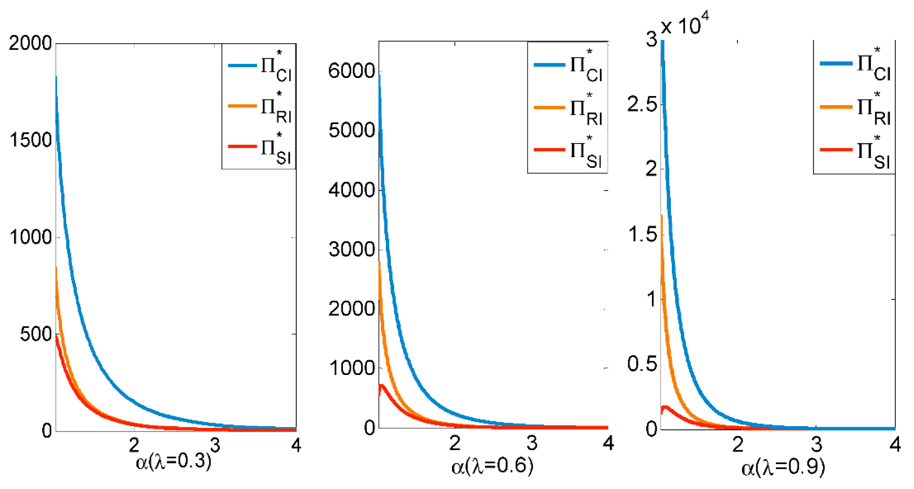
5.1. Economic Sustainability

According to Choi and Chiu [25], economic sustainability is closely related to profitability. For the existence of a double marginal effect, the profit in the decentralized supply chain is always lower than that in the CI. Therefore, we take the supply-chain efficiency to measure the economic sustainability of the supply chain. Referencing Wang et al. [61], we denote the efficiency of the decentralized supply chain equals the ratio of its profits compared with the profits in the CI. Then, the efficiency of the decentralized supply chain in Scenario SI and Scenario RI are as follows:

$${\Delta }_{\mathrm{S}\mathrm{I}}^{*}=\frac{{\mathsf{\Pi }}_{\mathrm{S}\mathrm{I}}^{*}}{{\mathsf{\Pi }}_{\mathrm{C}\mathrm{I}}^{*}}=\frac{{\mathsf{\Pi }}_{\mathrm{S}\mathrm{I}}^{\mathrm{S}*}+{\mathsf{\Pi }}_{\mathrm{S}\mathrm{I}}^{\mathrm{R}*}}{{\mathsf{\Pi }}_{\mathrm{C}\mathrm{I}}^{*}}=\frac{\left(2\alpha +\left(2-\lambda \right)\left(\alpha -1\right)\right){\left(\alpha -1\right)}^{\frac{2\alpha }{2-\lambda }}}{\left(2-\lambda \right)\left(\alpha -1\right){\left(\alpha \right)}^{\frac{2\alpha }{2-\lambda }}},$$

(34)

$${\Delta }_{\mathrm{R}\mathrm{I}}^{*}=\frac{{\mathsf{\Pi }}_{\mathrm{R}\mathrm{I}}^{*}}{{\mathsf{\Pi }}_{\mathrm{C}\mathrm{I}}^{*}}=\frac{{\mathsf{\Pi }}_{\mathrm{R}\mathrm{I}}^{\mathrm{S}*}+{\mathsf{\Pi }}_{\mathrm{R}\mathrm{I}}^{\mathrm{R}*}}{{\mathsf{\Pi }}_{\mathrm{C}\mathrm{I}}^{*}}=\frac{\left(2\alpha +\left(2-\lambda \right)\left(\alpha -1\right)\right){\left(\alpha -1\right)}^{\frac{2\left(\alpha -1\right)}{2-\lambda }}}{\left(2-\lambda \right)\left(\alpha -1\right){\left(\alpha \right)}^{\frac{2\left(\alpha -1\right)}{2-\lambda }}}.$$

(35)

Proposition 9. 

(1)${\Delta }_{\mathrm{R}\mathrm{I}}^{*}>{\Delta }_{\mathrm{S}\mathrm{I}}^{*}$always holds; (2) if$\gamma ={\Delta }_{\mathrm{R}\mathrm{I}}^{*}/{\Delta }_{\mathrm{S}\mathrm{I}}^{*}$,$\gamma$increases with$\lambda$increasing and decreases with$\alpha$increasing.

Proposition 9(1) shows that the retailer’s investments in green technology are more conducive to the overall performance and economic sustainability of the decentralized supply chain. This is because retailers’ investments in green technology can give them the first-mover advantage and reduce the decentralized supply chain’s double marginal effect. Figure 8 shows the supply chain’s profits in different scenarios, which verifies the conclusion above. (Aligned with the parameters set above, Figure 8 generates parameters settings as $\mathsf{\eta }=3$, $\mathsf{\mu }=2$, $\mathsf{\kappa }=300$, $\mathrm{c}=2$, and $\alpha =2$). Proposition 9(2) demonstrates that when the price elasticity is constant, the market demand is more sensitive to green technology investment level and retailer green technology investment is more beneficial to improving the performance of the decentralized supply chain. Oppositely, when demand elasticity of the green technology investment level is constant, the demand is less sensitive to price elasticity and retailer green technology investment is more beneficial to the decentralized supply chain’s performance. This is because green technology investment levels could be recognized as an adjustment method of supply-chain channel power. Therefore, the larger $\lambda$ is, the more sensitive the demand is to the green technology investment level, and green technology investment is more beneficial to improving the retailer’s supply-chain power and reducing the decentralized supply chain’s double marginal effect. As we know from Proposition 8, when the price elasticity is high, retailers will no longer be able to reverse their supply-chain power from the green technology investment because of the limited impact of green technology investment on market demand. Therefore, retailers will no longer take the initiative to invest in green technology.

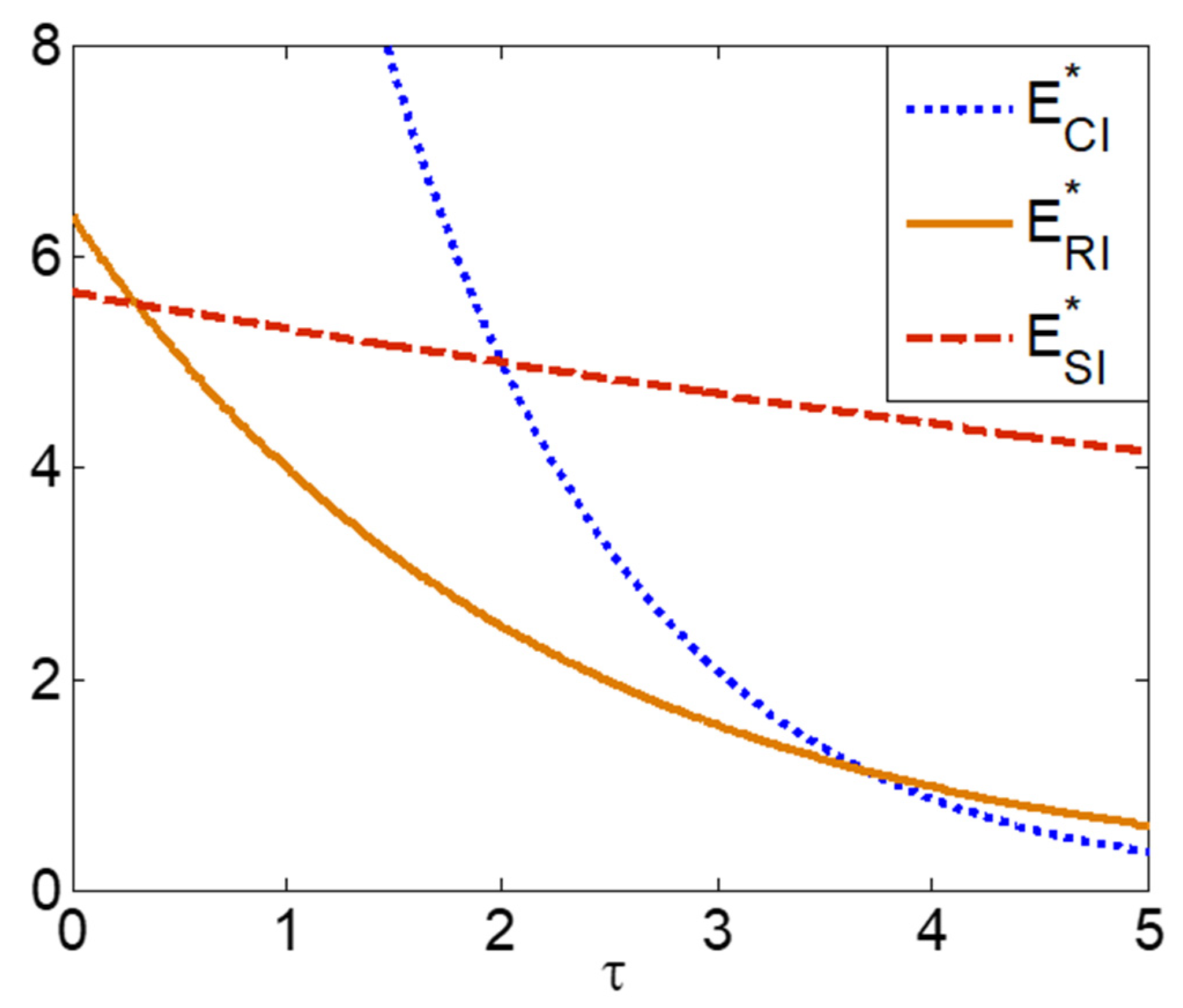
5.2. Environmental Sustainability

Referencing Krass et al. [27] and Niu et al. [46], we define the supply chain’s environmental impact. We can easily discover that the supply chain’s environmental impact positively correlates with the output and negatively correlates with the innovation level. We normalize the per-product pollution to 1. Then, the supply chain’s environmental impacts in different investment structures are formulated as follows:

$${\mathrm{E}}_{\mathrm{i}}=\frac{{\mathrm{Q}}_{\mathrm{i}}}{{\left(1+{\mathrm{s}}_{\mathrm{i}}\right)}^{\mathsf{\tau }}},$$

(36)

where $\mathrm{i}=\mathrm{C}\mathrm{I},\mathrm{R}\mathrm{I},\mathrm{o}\mathrm{r} \mathrm{S}\mathrm{I}$, and $\mathsf{\tau }$ is the elasticity of products’ pollution reduction to green technology investment.

Proposition 10. 

${\mathrm{E}}_{\mathrm{S}\mathrm{I}}^{*}>{\mathrm{E}}_{\mathrm{R}\mathrm{I}}^{*}>{\mathrm{E}}_{\mathrm{C}\mathrm{I}}^{*}$, if$\mathsf{\tau }\ge \frac{2\alpha -\lambda }{\alpha -1}$;${\mathrm{E}}_{\mathrm{S}\mathrm{I}}^{*}\ge {\mathrm{E}}_{\mathrm{C}\mathrm{I}}^{*}\ge {\mathrm{E}}_{\mathrm{R}\mathrm{I}}^{*}$, if$\frac{2\alpha -\lambda }{\alpha -1}\ge \mathsf{\tau }\ge 2$;${\mathrm{E}}_{\mathrm{C}\mathrm{I}}^{*}\ge {\mathrm{E}}_{\mathrm{S}\mathrm{I}}^{*}\ge {\mathrm{E}}_{\mathrm{R}\mathrm{I}}^{*}$, if$2\ge \mathsf{\tau }\ge \lambda$;${\mathrm{E}}_{\mathrm{C}\mathrm{I}}^{*}>{\mathrm{E}}_{\mathrm{R}\mathrm{I}}^{*}\ge {\mathrm{E}}_{\mathrm{S}\mathrm{I}}^{*}$, if$\lambda \ge \mathsf{\tau }>0$.

Proposition 10 suggests that investing in green technology does not always make the environment better, which some scholars call the “sustainable-effort-dilemma” [46]. The supply chain’s environmental impacts in different scenarios are shown as Figure 9 (Aligned with the parameters set above, Figure 9 generates parameters settings as $\mathsf{\eta }=3$, $\mathsf{\mu }=2$, $\mathsf{\kappa }=300$, $\mathrm{c}=2$, $\alpha =2$, and $\lambda =0.3$). We find that the key determinant of this dilemma in the decentralized supply chain is whether demand or environmental impact is more sensitive to green technology investment. That is to say, if environmental impact is more sensitive to green technology investment in the decentralized supply chain, green technology investment can reduce environmental pollution. However, if the demand is more sensitive to green technology investment, green technology investments can increase ecological pollution. We also find that, although the CI eliminates the double marginal effect and improves supply-chain efficiency, it is not always beneficial to the environment. The reason is that the centralized model leads to more sales; however, the CI can only improve the environment if the impact of green technology investment on the environment is very strong ($\mathsf{\tau }$ is high enough). This result aligns with the “sustainable-effort-dilemma” phenomenon which is proposed by Niu et al. [46].

6. Extension-Joint Investment Mechanism

In the analysis above, the supplier always wants the retailer to invest in green technology. However, the retailer is only willing to invest when the price elasticity coefficient $\alpha$ is relatively low. Then, when the price elasticity coefficient $\alpha$ is relatively high, can the supplier find a joint investment mechanism to induce the retailer to join in the green technology investment and realize the supply chain coordination or Pareto improvements?

This scenario is the same as the supplier providing a cost-sharing contract in Scenario SI, and we named it Scenario CTSI. The cost-sharing contract allows both the supplier and the retailer to jointly invest in green technology. That is, when the supplier and retailer enter into the contract agreement, the supplier and retailer share the green technology investment costs. We let $\mathsf{\theta }\in \left(0,1\right)$ be the fraction of the investment cost borne by the retailer, then, the left $1-\mathsf{\theta }$ fraction of the investment cost is borne by the supplier. Then, the profit functions of the supplier and retailer can be rewritten as follows:

$${\mathsf{\Pi }}_{\mathrm{C}\mathrm{T}\mathrm{S}\mathrm{I}}^{\mathrm{S}*}=\mathrm{E}[\mathrm{p}\mathrm{m}\mathrm{i}\mathrm{n}\left(\mathrm{D},\mathrm{Q}\right)+\left(\mathrm{w}-\mathrm{c}\right)\mathrm{Q}]-\frac{\mathsf{\eta }\left(1-\mathsf{\theta }\right)}{2}{\left(1+\mathrm{s}\right)}^2,$$

(37)

$${\mathsf{\Pi }}_{\mathrm{C}\mathrm{T}\mathrm{S}\mathrm{I}}^{\mathrm{R}*}=\mathrm{E}[\mathrm{p}\mathrm{m}\mathrm{i}\mathrm{n}\left(\mathrm{D},\mathrm{Q}\right)-\mathrm{w}\mathrm{Q}]-\frac{\mathsf{\eta }\mathsf{\theta }}{2}{\left(1+\mathrm{s}\right)}^2.$$

(38)

The sequence of the events in Scenario CTSI is similar to Scenario SI, the only difference is the supplier provides a cost-sharing contract before she decides the green technology investment level, and the retailer will need to bear the corresponding investment cost if he agrees with the contract. The timing of events in Scenario CTSI is shown in Figure 10.

Applying backward induction to solve the multistage game in this scenario. we can get the equilibrium decision variables and expectation equilibrium profits of the supply-chain members in Scenario CTSI as Proposition 11 presents.

Proposition 11. 

The decision variables and expected equilibrium profits of the supply-chain members in Scenario CTSI are summarized in

Table 6. The equilibrium results in model CTSI.

Scenario CTSI
${\mathrm{p}}_{\mathrm{C}\mathrm{T}\mathrm{S}\mathrm{I}}^{*}=\frac{\alpha \mathrm{c}\left(1+\alpha \right)}{{\left(\alpha -1\right)}^2}$	${\mathrm{Q}}_{\mathrm{C}\mathrm{T}\mathrm{S}\mathrm{I}}^{*}=\frac{4\mathsf{\mu }\mathsf{\kappa }{\left(\alpha -1\right)}^{2\alpha }}{{\alpha }^{\alpha }{\mathrm{c}}^{\alpha }{\left(1+\alpha \right)}^{\alpha +1}}{\left(\frac{4\mathsf{\kappa }\mathrm{u}\lambda {\left(\alpha -1\right)}^{2\alpha -1}}{\mathsf{\eta }\left(1-\mathsf{\theta }\right){\alpha }^{\alpha }{\mathrm{c}}^{\alpha -1}{\left(\mathrm{a}+1\right)}^{\alpha +1}}\right)}^{\frac{\lambda }{2-\lambda }}$
${\mathrm{w}}_{\mathrm{C}\mathrm{T}\mathrm{S}\mathrm{I}}^{*}=\frac{\alpha \mathrm{c}}{\alpha -1}$	$\mathrm{V}{\mathrm{Q}}_{\mathrm{C}\mathrm{T}\mathrm{S}\mathrm{I}}^{*}=\mathrm{m}\mathrm{a}\mathrm{x}\left\{\frac{\mathsf{\kappa }\left(3-\alpha \right)\mathsf{\mu }{\left(\alpha -1\right)}^{2\alpha }}{{\alpha }^{\alpha }{\mathrm{c}}^{\alpha }{\left(1+\alpha \right)}^{\alpha +1}}{\left(\frac{4\mathsf{\kappa }\mathrm{u}\lambda {\left(\alpha -1\right)}^{2\alpha -1}}{\mathsf{\eta }\left(1-\mathsf{\theta }\right){\alpha }^{\alpha }{\mathrm{c}}^{\alpha -1}{\left(\mathrm{a}+1\right)}^{\alpha +1}}\right)}^{\frac{\lambda }{2-\lambda }},0\right\}$
${\mathrm{s}}_{\mathrm{C}\mathrm{T}\mathrm{S}\mathrm{I}}^{*}=\mathrm{m}\mathrm{a}\mathrm{x}\left\{\sqrt[2-\lambda ]{\frac{4\mathsf{\kappa }\mathrm{u}\lambda {\left(\alpha -1\right)}^{2\alpha -1}}{\mathsf{\eta }\left(1-\mathsf{\theta }\right){\alpha }^{\alpha }{\mathrm{c}}^{\alpha -1}{\left(\mathrm{a}+1\right)}^{\alpha +1}}}-1,0\right\}$
${\mathsf{\Pi }}_{\mathrm{C}\mathrm{T}\mathrm{S}\mathrm{I}-\mathrm{N}}^{\mathrm{S}*}=\frac{2\mathsf{\kappa }\mathrm{u}{\left(\alpha -1\right)}^{2\alpha -1}}{{\alpha }^{\alpha }{\mathrm{c}}^{\alpha -1}{\left(\alpha +1\right)}^{\alpha +1}}$	${\mathsf{\Pi }}_{\mathrm{C}\mathrm{T}\mathrm{S}\mathrm{I}}^{\mathrm{S}*}=\frac{2\mathsf{\kappa }\mathrm{u}{\left(\alpha -1\right)}^{2\alpha -1}\left(2-\lambda \right){\left(4\mathsf{\kappa }\mathrm{u}\lambda {\left(\alpha -1\right)}^{2\alpha -1}\right)}^{\frac{\lambda }{2-\lambda }}}{{\alpha }^{\alpha }{\mathrm{c}}^{\alpha -1}{\left(\alpha +1\right)}^{\alpha +1}{\left(\mathsf{\eta }\left(1-\mathsf{\theta }\right){\alpha }^{\alpha }{\mathrm{c}}^{\alpha -1}{\left(\alpha +1\right)}^{\alpha +1}\right)}^{\frac{\lambda }{2-\lambda }}}$
${\mathsf{\Pi }}_{\mathrm{C}\mathrm{T}\mathrm{S}\mathrm{I}}^{\mathrm{R}*}=\frac{4\alpha \mathsf{\kappa }\mathrm{u}{\left(\alpha -1\right)}^{2\alpha -2}}{{\alpha }^{\alpha }{\mathrm{c}}^{\alpha -1}{\left(\alpha +1\right)}^{\alpha +1}}$	${\mathsf{\Pi }}_{\mathrm{C}\mathrm{T}\mathrm{S}\mathrm{I}}^{\mathrm{R}*}=\frac{2\mathsf{\kappa }\mathrm{u}\left(2\alpha -\lambda \left(\alpha -1\right)\frac{\mathsf{\theta }}{\left(1-\mathsf{\theta }\right)}\right){\left(\alpha -1\right)}^{2\alpha -2}{\left(4\mathsf{\kappa }\mathrm{u}\lambda {\left(\alpha -1\right)}^{2\alpha -1}\right)}^{\frac{\lambda }{2-\lambda }}}{{\alpha }^{\alpha }{\mathrm{c}}^{\alpha -1}{\left(\alpha +1\right)}^{\alpha +1}{\left(\mathsf{\eta }\left(1-\mathsf{\theta }\right){\alpha }^{\alpha }{\mathrm{c}}^{\alpha -1}{\left(\alpha +1\right)}^{\alpha +1}\right)}^{\frac{\lambda }{2-\lambda }}}$

.

Corollary 4. 

No matter if the supplier or the retailer decides the green technology investment level, the cost-sharing contract could not achieve supply chain perfect coordination.

Corollary 4 is an important finding. The equilibrium price in Scenario CTSI is the same as that in Scenario SI, which is independent of the green technology investment cost when the supply chain members agree with a cost-sharing contract. Based on the analysis in Section 3, we could infer that the supply chain would also not achieve perfect coordination when the retailer decides the green technology investment level. It proves once again that the purpose of supply chain members investing in green technology is to expand sales volume. However, that could not eliminate the double marginal effect.

Next, comparing the equilibrium profits in Scenario CTSI and Scenario SI, we can get Proposition 11.

Proposition 12. 

(1) With a cost-sharing mechanism, the Pareto zone is$\left(0,{\overline{\mathsf{\theta }}}_{\mathrm{C}\mathrm{T}\mathrm{S}\mathrm{I}}\right)$, where$\overline{\mathsf{\theta }}$meets the condition$\lambda \left(\alpha -1\right){\overline{\mathsf{\theta }}}_{\mathrm{C}\mathrm{T}\mathrm{S}\mathrm{I}}=2\alpha \left[\left(1-{\overline{\mathsf{\theta }}}_{\mathrm{C}\mathrm{T}\mathrm{S}\mathrm{I}}\right)-{\left(1-{\overline{\mathsf{\theta }}}_{\mathrm{C}\mathrm{T}\mathrm{S}\mathrm{I}}\right)}^{\frac{2}{2-\lambda }}\right]$. (2) Within the Pareto zone,${\mathrm{s}}_{\mathrm{C}\mathrm{T}\mathrm{S}\mathrm{I}}^{*}$increases with$\mathsf{\theta }$. (3) Within the Pareto zone, with the increasing of$\mathsf{\theta }$,${\mathsf{\Pi }}_{\mathrm{C}\mathrm{T}\mathrm{S}\mathrm{I}}^{\mathrm{S}*}$always increases, while${\mathsf{\Pi }}_{\mathrm{C}\mathrm{T}\mathrm{S}\mathrm{I}}^{\mathrm{R}*}$increases first, then decreases.

Proposition 11 demonstrates that a cost-sharing contract can always be designed to enable the supplier and retailer to achieve Pareto improvements in Scenario CTSI. Within the Pareto zone, with an increase of the green technology investment cost borne by the retailer, the green technology investment levels increase. The profits of the supplier and retailer also increase, which is shown in Figure 11 (Aligned with the parameters set above, Figure 11 generates parameters settings as $\mathsf{\eta }=3$, $\mathsf{\mu }=2$, $\mathsf{\kappa }=300$, $\mathrm{c}=2$, $\alpha =2$, and $\lambda =0.3$). This is because the marginal benefit of suppliers’ green technology investment will increase when the retailer bears part of the cost of green technology investment, and so too does the profitability of green technology investment. Therefore, the supplier will increase the green technology investment level. The higher the proportion of investment borne by the retailer, the higher the green technology investment level is and the higher profits of the supplier. In the Pareto zone, a marginal return of the retailer’s green technology investment is first positive, then negative with increasing cost-sharing proportion, and, therefore, the profit of the retailer first increases then decreases. Above all, when the retailer has no intention to invest in green technology, the supplier can always design a cost-sharing contract to induce the retailer to join the investment and increase both profits.

Additionally, there is no need to discuss the scenario with a cost-sharing contract when the retailer decides the green technology investment level. Due to the analysis above, we know that the retailer’s efficiency of green technology investment is higher than the supplier’s. That means, when the retailer voluntarily invests in green technology, the supplier part in the investment will not bring higher efficiency, and will not realize a Pareto improvement of the supply chain.

7. Conclusions

The green technology investment undertaken by different inventors in the decentralized supply chain can have different effects on the investment level, profits, and supply-chain sustainability. In this paper, we considered a supply chain that consists of an upstream supplier and a downstream retailer. We study the influence of different investment bodies of green technology on supply-chain operation and sustainability.

The results show that, compared to the supplier, the retailer has the stronger motivation to invest in green technology. Besides, both the supplier and retailer should intuitively want each other to invest in green technology. However, the results show that the retailer’s investment behavior is somewhat counterintuitive; the retailer tends to invest in green technology himself when customers are not so sensitive to the products’ retail prices. At the same time, we find that when retailers invest in green technology, the level of investment, as well as the order quantity and leftovers in the decentralized supply chain are higher. However, the retail price is the same no matter who invests in green technology. This result is different from that in a scenario with determined and line demand and competition proposed by Shi et al. [41]. This is because the purpose of green technology investment in these uncertain circumstances is only to expand sales volumes rather than increase prices. By comparing operations in the CI structure, we find that the supply chain has the highest inventory utilization and the lower retail price. That is, the order quantity in the centralized-decision supply-chain structure is significantly higher than that in the decentralized-decision supply-chain structure. However, the difference of leftovers in decentralized supply-chain structures is not that obvious. More importantly, we find the supply chain could not realize perfect coordination no matter who decides the green technology investment level. When the retailer has no intention of investing in green technology, the supplier can always design a cost-sharing contract to induce the retailer to join in the green technology investment and realize a Pareto improvement of the supply chain.

Regarding supply-chain sustainability, the decentralized supply chain always loses parts of supply-chain economic efficiency for the existence of double marginalization. It is more economically efficient for downstream enterprises to invest in green technology than upstream ones, and the motivation to invest is also stronger. Significantly, high levels of green technology investments are not necessarily good for the environment. In the decentralized supply chain, only when the environmental impact is more sensitive to green technology investment is investing in green technology good for the environment. However, the CI requires pollution emissions to be more sensitive to green technology investments to improve the environment. That aligns with the “sustainable-effort-dilemma” phenomenon which is proposed by Niu et al. [46].

The results of this paper provide a theoretical reference for the supply chain members to make decisions on green technology investment, the supplier inducing the retailer to join in the investment through a cost-sharing contract, and the relevant departments managing the sustainability of the production.

There are still certain limitations in this study, and some important extensions can be considered in future research. First, to focus on whether the upstream or downstream should invest in green technology investment under uncertainty, this paper considers the supply chain with one supplier and one retailer as the subject. In practice, it is common to see multiple suppliers serve one retailer, or one supplier serve many retailers. We will consider different supply chain structures in future research. Second, the risk preference of the investor is also an important factor that influences green technology investment level, operation decisions, and profits of supply chain parties in an uncertain environment. Thus, introducing risk preference into our models for future research is worthwhile. Third, this study analyzes environmental sustainability from the perspective of total production. Future research needs to subdivide the environmental impact of green technology investment on each production procedure, and use effective data and control methods, such as anomaly detection [65] and stochastic control approach [66], to make more targeted investments and maximize both the economic and environmental return in green technology. Finally, we design a joint investment mechanism with a cost-sharing contract, which realizes the Pareto improvement of the supply chain. Another direction for our further research could focus on incentive mechanisms involving competition or risk preference under uncertain demand.

References

1. Ahi, P.; Searcy, C. A comparative literature analysis of definitions for green and sustainable supply chain management. J. Clean. Prod. 2013, 52, 329–341. [Google Scholar] [CrossRef]
2. Subramanian, N.; Gunasekaran, A. Cleaner supply-chain management practices for twenty-first-century organizational competitiveness: Practice-performance framework and research propositions. Int. J. Prod. Econ. 2015, 164, 216–233. [Google Scholar] [CrossRef]
3. Martins, A. Most Consumers Want Sustainable Products and Packaging. Available online: https://www.businessnewsdaily.com/15087-consumers-want-sustainable-products.html (accessed on 5 June 2019).
4. Genc, T.S.; De, G.P. Closed-loop supply chain games with innovation-led lean programs and sustainability. Int. J. Prod. Econ. 2020, 219, 440–456. [Google Scholar] [CrossRef]
5. Ball, P.; Lunt, P. Lean eco-efficient innovation in operations through the maintenance organisation. Int. J. Prod. Econ. 2020, 219, 405–415. [Google Scholar] [CrossRef]
6. Xu, X.; He, P.; Xu, H.; Zhang, Q. Supply chain coordination with green technology under cap-and-trade regulation. Int. J. Prod. Econ. 2017, 183, 433–442. [Google Scholar] [CrossRef]
7. Lin, B.; Zhu, F.; Zhang, J.; Chen, J.; Chen, X.; Xiong, N.N.; Mauri, J.L. A Time-Driven Data Placement Strategy for a Scientific Workflow Combining Edge Computing and Cloud Computing. IEEE Trans. Ind. Inform. 2019, 15, 4254–4265. [Google Scholar] [CrossRef] [Green Version]
8. Yi, B.; Shen, X.; Liu, H.; Zhang, Z.; Zhang, W.; Liu, S.; Xiong, N. Deep Matrix Factorization with Implicit Feedback Embedding for Recommendation System. IEEE Trans. Ind. Inform. 2019, 15, 4591–4601. [Google Scholar] [CrossRef]
9. Qu, Y.; Xiong, N. RFH: A Resilient, Fault-Tolerant and High-Efficient Replication Algorithm for Distributed Cloud Storage. In Proceedings of the 2012 41st International Conference on Parallel Processing, Pittsburgh, PA, USA, 25 October 2012. [Google Scholar]
10. Li, H.; Liu, J.; Liu, R.W.; Xiong, N.; Wu, K.; Kim, T.-H. A Dimensionality Reduction-Based Multi-Step Clustering Method for Robust Vessel Trajectory Analysis. Sensors 2017, 17, 1792. [Google Scholar] [CrossRef] [Green Version]
11. Jabbour, C.J.C.; Neto, A.S.; Gobbo, J.A.; Ribeiro, M.D.S.; Jabbour, A.B.L.D.S. Eco-innovations in more sustainable supply chains for a low-carbon economy: A multiple case study of human critical success factors in Brazilian leading companies. Int. J. Prod. Econ. 2015, 164, 245–257. [Google Scholar] [CrossRef]
12. Yu, Y.; Han, X.; Hu, P. Optimal production for manufacturers considering consumer environmental awareness and green subsidies. Int. J. Prod. Econ. 2016, 182, 397–408. [Google Scholar] [CrossRef] [Green Version]
13. Gassmann, O.; Zeschky, M.; Wolff, T.; Stahl, M. Crossing the Industry-Line: Breakthrough Innovation through Cross-Industry Alliances with ‘Non-Suppliers’. Long Range Plan. 2010, 43, 639–654. [Google Scholar] [CrossRef]
14. Laseter, T.M.; Ramdas, K. Product Types and Supplier Roles in Product Development: An Exploratory Analysis. SSRN Electron. J. 2001, 49, 107–118. [Google Scholar] [CrossRef]
15. Flynn, B.B.; Koufteros, X.; Lu, G. On Theory in Supply Chain Uncertainty and its Implications for Supply Chain Integration. J. Supply Chain Manag. 2016, 52, 3–27. [Google Scholar] [CrossRef] [Green Version]
16. Krause, D.R.; Vachon, S.; Klassen, R.D. Special topic forum on sustainable supply chain management: Introduction and reflections on the role of purchasing management. J. Supply Chain Manag. 2009, 45, 18–25. [Google Scholar] [CrossRef]
17. Wu, Z.; Pagell, M. Balancing priorities: Decision-making in sustainable supply chain management. J. Oper. Manag. 2010, 29, 577–590. [Google Scholar] [CrossRef]
18. Niu, B.; Chen, L.; Zhang, J. Punishing or subsidizing? Regulation analysis of sustainable fashion procurement strategies. Transp. Res. Part E Logist. Transp. Rev. 2017, 107, 81–96. [Google Scholar] [CrossRef]
19. Ye, F.; Li, Y.; Yang, Q. Designing coordination contract for biofuel supply chain in China. Resour. Conserv. Recycl. 2018, 128, 306–314. [Google Scholar] [CrossRef]
20. Ma, W.; Zhang, R.; Chai, S. What Drives Green Innovation? A Game Theoretic Analysis of Government Subsidy and Cooperation Contract. Sustainability 2019, 11, 5584. [Google Scholar] [CrossRef] [Green Version]
21. Xue, J.; Gong, R.; Zhao, L.; Ji, X.; Xu, Y. A Green Supply-Chain Decision Model for Energy-Saving Products That Accounts for Government Subsidies. Sustainability 2019, 11, 2209. [Google Scholar] [CrossRef] [Green Version]
22. Ghosh, D.; Shah, J. Supply chain analysis under green sensitive consumer demand and cost sharing contract. Int. J. Prod. Econ. 2015, 164, 319–329. [Google Scholar] [CrossRef]
23. Saha, S.; Goyal, S. Supply chain coordination contracts with inventory level and retail price dependent demand. Int. J. Prod. Econ. 2015, 161, 140–152. [Google Scholar] [CrossRef]
24. Yenipazarli, A. To collaborate or not to collaborate: Prompting upstream eco-efficient innovation in a supply chain. Eur. J. Oper. Res. 2017, 260, 571–587. [Google Scholar] [CrossRef]
25. Choi, T.-M.; Chiu, C.-H. Mean-downside-risk and mean-variance newsvendor models: Implications for sustainable fashion retailing. Int. J. Prod. Econ. 2012, 135, 552–560. [Google Scholar] [CrossRef]
26. Ma, W.; Cheng, Z.; Xu, S. A Game Theoretic Approach for Improving Environmental and Economic Performance in a Dual-Channel Green Supply Chain. Sustainability 2018, 10, 1918. [Google Scholar] [CrossRef] [Green Version]
27. Krass, D.; Nedorezov, T.; Ovchinnikov, A. Environmental Taxes and the Choice of Green Technology. Prod. Oper. Manag. 2013, 22, 1035–1055. [Google Scholar] [CrossRef]
28. Tang, L.; Shi, J.; Yu, L.; Bao, Q. Economic and environmental influences of coal resource tax in China: A dynamic computable general equilibrium approach. Resour. Conserv. Recycl. 2017, 117, 34–44. [Google Scholar] [CrossRef]
29. Hong, Z.; Guo, X. Green product supply chain contracts considering environmental responsibilities. Omega 2019, 83, 155–166. [Google Scholar] [CrossRef]
30. Shen, B.; Li, Q. Impacts of Returning Unsold Products in Retail Outsourcing Fashion Supply Chain: A Sustainability Analysis. Sustainability 2015, 7, 1172–1185. [Google Scholar] [CrossRef] [Green Version]
31. Leitão, J.; Pereira, D.; De Brito, S. Inbound and Outbound Practices of Open Innovation and Eco-Innovation: Contrasting Bioeconomy and Non-Bioeconomy Firms. J. Open Innov. Technol. Mark. Complex. 2020, 6, 145. [Google Scholar] [CrossRef]
32. Li, Q.; Zhang, Z.; Rao, W.; Xu, W.; Jiang, L. Green Investment Decisions in Supply Chains: A Game Model with Complete Information. Information 2019, 10, 185. [Google Scholar] [CrossRef] [Green Version]
33. Govindan, K.; Popiuc, M.N. Reverse supply chain coordination by revenue sharing contract: A case for the personal computers industry. Eur. J. Oper. Res. 2014, 233, 326–336. [Google Scholar] [CrossRef]
34. Nesticò, A.; Galante, M. An estimate model for the equalisation of real estate tax: A case study. Int. J. Bus. Intell. Data Min. 2015, 10, 19–32. [Google Scholar] [CrossRef]
35. Niu, B.; Liu, Y.; Luo, H.; Feng, B. Domestic sourcing vs. cross-border sourcing: Impact of the quality of the scrap metal and Government’s tariff policies. J. Clean. Prod. 2019, 208, 1281–1293. [Google Scholar] [CrossRef]
36. Janeiro, L.; Patel, M.K. Choosing sustainable technologies. Implications of the underlying sustainability paradigm in the decision-making process. J. Clean. Prod. 2015, 105, 438–446. [Google Scholar] [CrossRef]
37. Bai, C.; Satir, A.; Sarkis, J. Investing in lean manufacturing practices: An environmental and operational perspective. Int. J. Prod. Res. 2018, 57, 1037–1051. [Google Scholar] [CrossRef]
38. Meng, Q.; Wang, Y.; Zhang, Z.; He, Y. Supply chain green innovation subsidy strategy considering consumer heterogeneity. J. Clean. Prod. 2021, 281, 125199. [Google Scholar] [CrossRef]
39. Silvestre, B.S. Sustainable supply chain management in emerging economies: Environmental turbulence, institutional voids and sustainability trajectories. Int. J. Prod. Econ. 2015, 167, 156–169. [Google Scholar] [CrossRef]
40. Xing, G.; Xia, B.; Guo, J. Sustainable Cooperation in the Green Supply Chain under Financial Constraints. Sustainability 2019, 11, 5977. [Google Scholar] [CrossRef] [Green Version]
41. Shi, X.; Dong, C.; Zhang, C.; Zhang, X. Who should invest in clean technologies in a supply chain with competition? J. Clean. Prod. 2019, 215, 689–700. [Google Scholar] [CrossRef]
42. Hall, J.; Matos, S.; Silvestre, B. Understanding why firms should invest in sustainable supply chains: A complexity approach. Int. J. Prod. Res. 2012, 50, 1332–1348. [Google Scholar] [CrossRef]
43. Chan, H.K.; Yee, R.W.; Dai, J.; Lim, M.K. The moderating effect of environmental dynamism on green product innovation and performance. Int. J. Prod. Econ. 2016, 181, 384–391. [Google Scholar] [CrossRef]
44. Ba, S.; Ling, L.; Liu, Q.; Stallaert, J. Stock Market Reaction to Green Vehicle Innovation. Prod. Oper. Manag. 2013, 22, 976–990. [Google Scholar] [CrossRef]
45. Lin, R.-J.; Tan, K.-H.; Geng, Y. Market demand, green product innovation, and firm performance: Evidence from Vietnam motorcycle industry. J. Clean. Prod. 2013, 40, 101–107. [Google Scholar] [CrossRef]
46. Niu, B.; Mu, Z.; Chen, L.; Lee, C.K. Coordinate the economic and environmental sustainability via procurement outsourcing in a co-opetitive supply chain. Resour. Conserv. Recycl. 2019, 146, 17–27. [Google Scholar] [CrossRef]
47. Wang, Y.; Niu, B.; Guo, P. On the Advantage of Quantity Leadership When Outsourcing Production to a Competitive Contract Manufacturer. Prod. Oper. Manag. 2012, 22, 104–119. [Google Scholar] [CrossRef]
48. Wu, J.; Fan, J.; He, Y. Pricing and horizontal information sharing in a supply chain with capacity constraint. Oper. Res. Lett. 2018, 46, 402–408. [Google Scholar] [CrossRef]
49. Matsui, K. When should a manufacturer set its direct price and wholesale price in dual-channel supply chains? Eur. J. Oper. Res. 2017, 258, 501–511. [Google Scholar] [CrossRef] [Green Version]
50. Zhao, J.; Wei, J.; Li, Y. Pricing decisions for substitutable products in a two-echelon supply chain with firms’ different channel powers. Int. J. Prod. Econ. 2014, 153, 243–252. [Google Scholar] [CrossRef]
51. Chen, X.; Zhang, H.; Zhang, M.; Chen, J. Optimal decisions in a retailer Stackelberg supply chain. Int. J. Prod. Econ. 2017, 187, 260–270. [Google Scholar] [CrossRef]
52. Chernonog, T. Inventory and marketing policy in a supply chain of a perishable product. Int. J. Prod. Econ. 2020, 219, 259–274. [Google Scholar] [CrossRef]
53. Albrecht, M. Determining near optimal base-stock levels in two-stage general inventory systems. Eur. J. Oper. Res. 2014, 232, 342–349. [Google Scholar] [CrossRef]
54. Shafiq, M.; Savino, M.M. Supply chain coordination to optimize manufacturer’s capacity procurement decisions through a new commitment-based model with penalty and revenue-sharing. Int. J. Prod. Econ. 2019, 208, 512–528. [Google Scholar] [CrossRef]
55. Bhaskaran, S.R.; Krishnan, V. Effort, Revenue, and Cost Sharing Mechanisms for Collaborative New Product Development. Manag. Sci. 2009, 55, 1152–1169. [Google Scholar] [CrossRef] [Green Version]
56. Liu, X.; Lin, K.; Wang, L.; Ding, L. Pricing Decisions for a Sustainable Supply Chain in the Presence of Potential Strategic Customers. Sustainabillity 2020, 12, 1655. [Google Scholar] [CrossRef] [Green Version]
57. Gong, B.; Xia, X.; Cheng, J. Supply-Chain Pricing and Coordination for New Energy Vehicles Considering Heterogeneity in Consumers’ Low Carbon Preference. Sustainability 2020, 12, 1306. [Google Scholar] [CrossRef] [Green Version]
58. González, A.B.R.; Díaz, J.J.V.; Wilby, M.R. Dedicated tax/subsidy scheme for reducing emissions by promoting innovation in buildings: The EcoTax. Energy Policy 2012, 51, 417–424. [Google Scholar] [CrossRef]
59. Liu, Z.; Li, X.; Peng, X.; Lee, S. Green or nongreen innovation? Different strategic preferences among subsidized enterprises with different ownership types. J. Clean. Prod. 2020, 245, 118786. [Google Scholar] [CrossRef]
60. Kyparisis, G.J.; Koulamas, C. Resale price maintenance in supply chains with general multiplicatyive demand. Oper. Res. Lett. 2018. [Google Scholar] [CrossRef]
61. Wang, Y.; Jiang, L.; Shen, Z. Channel Performance under Consignment Contract with Revenue Sharing. Manag. Sci. 2004, 50, 34–47. [Google Scholar] [CrossRef]
62. Li, Y.; Xu, L.; Li, D. Examining relationships between the return policy, product quality, and pricing strategy in online direct selling. Int. J. Prod. Econ. 2013, 144, 451–460. [Google Scholar] [CrossRef]
63. Dong, C.; Shen, B.; Chow, P.-S.; Yang, L.; Ng, C.T. Sustainability investment under cap-and-trade regulation. Ann. Oper. Res. 2016, 240, 509–531. [Google Scholar] [CrossRef]
64. Wang, Y. Joint Pricing-Production Decisions in Supply Chains of Complementary Products with Uncertain Demand. Oper. Res. 2006, 54, 1110–1127. [Google Scholar] [CrossRef]
65. Sun, J.; Wang, X.; Xiong, N.; Shao, J. Learning Sparse Representation with Variational Auto-Encoder for Anomaly Detection. IEEE Access 2018, 6, 33353–33361. [Google Scholar] [CrossRef]
66. Fang, W.; Yao, X.; Zhao, X.; Yin, J.; Xiong, N. A Stochastic Control Approach to Maximize Profit on Service Provisioning for Mobile Cloudlet Platforms. IEEE Trans. Syst. Man Cybern. Syst. 2016, 48, 522–534. [Google Scholar] [CrossRef]
Figure 1. The timing of the events in Scenario CI.
Sustainability 13 03752 g001
Figure 2. The timing of the events in Scenario SI.
Sustainability 13 03752 g002
Figure 3. The timing of the events in Scenario RI.
Sustainability 13 03752 g003
Figure 4. Green technology investment levels change in different scenarios.
Sustainability 13 03752 g004
Figure 5. Order quantity change in different scenarios.
Sustainability 13 03752 g005
Figure 6. Leftovers change in different scenarios.
Sustainability 13 03752 g006
Figure 7. Investment willingness area distribution.
Sustainability 13 03752 g007
Figure 8. The supply chain’s profits in different scenarios.
Sustainability 13 03752 g008
Figure 9. The supply chain’s environmental impacts in different scenarios.
Sustainability 13 03752 g009
Figure 10. The timing of the events in Scenario CTSI.
Sustainability 13 03752 g010
Figure 11. Profits of the supplier and retailer change in Scenario CTSI.
Sustainability 13 03752 g011