Abstract
This paper investigates whether energy consumption, population density, and exports are the main factors causing environmental damage in China. Using annual data from 1971–2018, unit root tests are applied for the stationarity analyses, and Autoregressive Distributed Lag (ARDL) bounds tests are used for the long-run relationships between the variables. A Vector Error Correction Model (VECM) Granger approach is employed to examine the causal relationships amongst the variables. Our findings show that the selected variables are cointegrated, and that energy consumption and economic growth are identified as the main reasons for CO2 emissions in both the short-run and long-run. In contrast, exports reduce CO2 emissions in the long-run. Short-run unidirectional Granger causality is found from economic growth to energy consumption, CO2 emissions and exports, and from CO2 emissions to energy consumption and exports. Moreover, long-run causal links exist between CO2 emissions and exports. Five policy recommendations are made following the obtained results.
JEL Classifications:
Q43; Q53; Q56; C22; O44
1. Introduction
China has attained remarkable achievements in a number of important areas during the last several decades. The real Gross Domestic Product (GDP, constant 2010 USD) per capita of China increased dramatically from USD 191.8 in 1960 to USD 8254 in 2019. The poverty headcount ratio of USD 1.9 a day decreased rapidly from 42.5% in 1981 to 9.2% in 2017. China is also the most populous country, with 1.44 billion people in 2020 [1], the highest consumer of energy, and the largest contributor of CO2 emissions, with 24% of global energy consumption and 29% of total CO2 emissions in 2018 [1]. The CO2 emissions of China (metric tons per capita) increased significantly, from 1.17 in 1960 to 7.95 in 2018 [1,2]. Therefore, it is useful to explore the causative factors of CO2 emissions in China.
A number of previous studies have identified energy consumption, economic growth, financial development, foreign direct investment, and trade openness as the major causative factors for environmental damage across countries; however, no previous studies, to the best of our knowledge, have investigated whether population density, along with other factors, is the main reason for environmental damage in China. Greater population means more human activities and a greater demand for industrial production, transport, and energy consumption that result in environmental degradation via increased CO2 emissions and huge amounts of waste [3]. Furthermore, export, rather than total trade or trade openness, is a more appropriate variable to consider in carbon analysis, because one-third of China’s CO2 emissions are caused by exports [4]. Surprisingly few studies in the past have explored the true effect of this variable on CO2 emissions. In this research, we have explored the roles of these two variables to fill the gaps in the literature. Hence, the novelty of this research is to explore the environmental effects of these two variables, which were previously ignored by other researchers. Our central question of investigation is: do these two new variables play any role in the environmental quality of China, along with other variables?
With this objective in mind, we have examined the effects of energy consumption, economic growth, exports, and population density on CO2 emissions (proxy for environmental quality) in China using the autoregressive distributive lag (ARDL) bounds tests and the VECM Granger causality technique. The main contributions of this study are as follows: (i) We add population density and exports as new variables to provide evidence of the linkages between economic growth, energy consumption, population density, exports, and CO2 emissions in China, in both the short- and long-run, which are limited in the literature to date; (ii) we conduct necessary diagnostic tests for checking the stationarity of variables, the reliability of the model, the stability of coefficients/results along with normality, and the serial correlation and heteroscedasticity tests; (iii) finally, we have initiated discussions for China on whether it should aim for continuous increased production using nonrenewable energy, or whether it should limit its growth aspirations by achieving sustainable production using more renewable energy and energy efficient technologies.
This study is important for the policy makers of China and other countries to understand the complex nexus between energy consumption, population density, exports, economic growth, and environmental quality for formulating effective policies for development. For instance, if population density and exports do adversely affect CO2 emissions, the government should redesign its trade policy for desired exports and do likewise with its population policy to have an optimum population by birth control and/or controlling migration. Similarly, if economic growth and energy consumption increase CO2 emissions, limiting growth targets by optimum production, and less use of nonrenewable energy and energy-inefficient technologies, would be effective options. Despite the negative impacts of the COVID-19 pandemic on the Chinese economy, it may be a new opportunity to restructure industries towards a digital and green economy, rather than restart traditional industries.
2. Literature Review
Some studies on the determinants of CO2 emissions have been conducted across countries; however, the findings are diverse, mainly due to the use of different methodological approaches and variables, data periods, and heterogeneous country characteristics. In this paper we will review past studies under four strands of research.
2.1. CO2 Emissions and Economic Growth Nexus
The theoretical framework of the Environmental Kuznets Curve (EKC) hypothesis is tested by the nexus between CO2 emissions and economic growth. According to this hypothesis, EKC is a nonlinear inverted U-shaped curve that explains that environmental degradation rises initially with the increase of economic growth, and then starts to decline when economic growth reaches a threshold with a high level of income [5]. This hypothesis implies that, in the long-run, economic growth brings welfare for the environment [6]. Although this hypothesis has been empirically tested by many researchers in single and cross-country studies, the researchers were unable to reach a conclusive agreement. For example, recent studies, such as those of Sarkodie and Ozturk [7], Rahman and Velayutham [8], Rahman, Murad [9], Shahbaz, Nasir [10], Zoundi [11], Lean and Smyth [12], Tiwari, Shahbaz [13], Ertugrul, Cetin [14], Kanjilal and Ghosh [15], and Sephton and Mann [16], found evidence of the existence of the EKC hypothesis. However, some studies, such as those of Rahman [17], Arouri, Youssef [18], Ozturk and Acaravci [19], Musolesi, Mazzanti [20], Pao, Yu [21], He and Richard [22], and Tunç, Türüt-Aşık [23], could not find compelling evidence for this hypothesis. Rahman [17] found a U-shaped relationship; Tunç, Türüt-Aşık [23], Kashem and Rahman [24], Arouri, Youssef [18], and Musolesi, Mazzanti [20] revealed an increasing long-run linear relationship between economic growth and CO2 emissions. Ozturk and Acaravci [19] and Musolesi, Mazzanti [20] found evidence of a U-shaped relationship between these two variables.
2.2. CO2 Emissions, Economic Growth and Energy Consumption Nexus
The nexus between CO2 emissions, economic growth, and energy consumption, as discussed in the current empirical literature, is also not uniform. For example, Alam, Begum [25], Appiah [26], Alam, Begum [27], Koengkan, Losekann [28], and Koengkan, Fuinhas [29] found a bidirectional causal link between CO2 emissions and energy consumption for India, Ghana, Bangladesh, four Andean community countries and five countries, including Argentina, Brazil, Paraguay, Uruguay, and Venezuela, respectively. However, no causality between economic growth and CO2 emissions was found in India, though a unidirectional causality running from CO2 emissions to economic growth was found in Bangladesh. On the other hand, some studies revealed the existence of unidirectional causality from economic growth to energy consumption and CO2 emissions (see Rahman and Kashem [30] for Bangladesh, Khan, Khan [31] for Pakistan, Uddin, Bidisha [32] for Sri Lanka, Kasman and Duman [33] for the EU members and candidate countries, Shahbaz, Hye [34] for Indonesia, and Hossain [35] for Japan). In addition, Adedoyin and Zakari [36] found a unidirectional causality from energy consumption to CO2 emissions for the United Kingdom. Likewise, positive effects of economic growth and energy consumption on CO2 emissions were confirmed by the studies of Balsalobre-Lorente, Shahbaz [37] for EU-5 countries, Ahmed, Bhattacharya [38] for ASEAN-8 countries, Begum, Sohag [39] for Malaysia, Tang and Tan [40] for Vietnam, and Alam, Murad [6] for other four countries. In Tunisia, Mbarek, Saidi [41] found a causal nexus between energy consumption and CO2 emissions. In contrast, Soytas, Sari [42] did not find any causal relationship between economic growth and CO2 emissions, and between energy and economic growth, in the USA.
2.3. CO2 Emissions and Population Density Nexus
Very few studies exist in the literature that examine the impact of population density/growth on CO2 emissions, though environmental quality is affected by population growth. Engelman [43] and O’Neill, MacKellar [44] opined that population growth is one of the major factors for CO2 emissions in all countries, irrespective of levels of development. Empirically, Mamun, Sohag [45] explored the link between population growth and CO2 emissions, controlling for some other variables, for a total of 136 countries, and revealed that population size increased CO2 emissions in the long-run. Ohlan [46] also indicated a significant positive impact of population density on CO2 emissions in India in short- and long-runs. In contrast, Chen, Wang [47] found that population density would reduce air pollution in China. Rahman, Saidi [48] revealed a unidirectional causality from population density to CO2 emissions for South Asia. Moreover, in a study on 93 countries, Shi [49] demonstrated that 1.28% of CO2 emissions are linked with 1% population growth, and that the extent of the impact of population increase on CO2 emissions is greater in developing countries than in developed countries.
2.4. CO2 Emissions–Trade/Exports Nexus
Theoretically, the net effect of international trade on environmental quality could either be beneficial or detrimental for the environment [17]. The supporters of a beneficial effect argue that free trade enables countries to have greater access to broader international markets. As a result, competition, power, and efficiency of countries are increased, which facilitates the import of cleaner technologies and, thus, lower carbon emissions [34,50]. On the other hand, negative arguments are raised by some researchers due to the fact that increased exports lead to increased industrial production activities, which ultimately increase CO2 emissions and, hence, damage environmental quality [51]. Empirically, Jebli, Youssef [52], Balsalobre-Lorente, Shahbaz [37], Gasimli, Gamage [53], Mahmood, Maalel [54], Murad and Mazumder [55], Tiwari, Shahbaz [13], and Halicioglu [56], found detrimental effects of trade on the environment in 22 Central and South American countries, 5 EU countries, as well as Sri Lanka, Tunisia, Malaysia, India, and Turkey. In contrast, Khan, Ali [57] demonstrated that exports decreased and imports increased consumption-based carbon emissions in nine oil-exporting countries. Similar findings are also found by Muhammad, Long [58] for 65 Belt and Road initiative countries. Furthermore, Haq, Zhu [59] and Shahbaz, Lean [60] found evidence of the beneficial effects of trade in Morocco and Pakistan. Likewise, Kasman and Duman [33] and Rahman, Saidi [61] investigated the causal relationship between trade openness and CO2 emissions in new EU member and candidate countries and three developed countries, although Haug and Ucal [62] and Hasanov, Liddle [63] found no or weak effects in Turkey and oil-exporting countries.
The forgoing discussion exhibits the contradictory nature about the responsible factors for CO2 emissions across countries. Therefore, country-specific studies focusing on appropriate variables, such as population density, are important to mitigate the current debate.
3. Materials and Methods
3.1. Theoretical Notions and the Model
The objective of our research was to investigate the impacts of population density, along with economic growth, energy consumption and export production, on CO2 emissions in China during the period 1971–2018. As energy consumption and economic growth may cause CO2 emissions [32,34,64] we included them in our model. We also added population density in our model because more people means higher demand for energy for elasticity, industrial activities, and transportation, all of which cause CO2 emissions [39,61]. In addition, we included export as a variable in our model, since it may affect environmental quality due to government policies, or may increase the income of developing countries and induce them to use/import environmentally friendly technology to promote production [34].
The rationale for selecting these variables is further discussed as follows. Kuznets [65] proposed that income disparity initially increases and declines with economic growth. The inclusion of economic growth in CO2 emissions analysis is based on the environmental Kuznets curve (EKC) hypothesis, which suggests that economic growth and environmental quality have an inverted U-shaped relationship. At the initial stages of industrialization and development, pollution levels increase with growth; however, growth may decrease pollution when countries are rich enough to pay for energy efficient and environment friendly technologies. Therefore, the model is constructed in a quadratic form of real GDP per capita.
In the same vein as capital and labor, energy is considered one of the important inputs of production. It is a vital instrument of socioeconomic development [66]. Energy consumption can both pollute the environment through the use of fossil fuels and improve environmental quality by renewable energy consumption. Fossil fuels are the major portion of energy use. For production activities, use of more machinery is needed, which requires more energy, emitting a greater amount of CO2 emissions in the atmosphere. In contrast, a number of alternative types of energy sources (e.g., wind, solar energy, nuclear power plants) do not add greenhouse gases to the atmosphere. Using these low carbon energy sources can reduce CO2 emissions.
High population density may cause several environmental impacts (see Section 2.3). For example, high population density can cause the depletion of natural resources (arable land, water, forest, energy, etc.) and degradation of the environment due to overuse of nonrenewable energy, for example, coal, oil, and natural gas [3].
From a theoretical point of view, the environmental impacts of international trade can be either positive or negative. Environmentalists believe that international trade affects the environment negatively, at least in the short-run, via international specialization in intensive polluting products, the acceleration of trade with hazardous substances and waste, and extensive transport use for long distances [67]. On the other hand, the positive effects of international trade on the environment are explained by the rationale that trade generates wealth and increases the movement of environmental technologies between countries [68]. As a result, a higher standard of living leads to higher demand for a cleaner environment, which will ultimately result in environmental improvement [69]. Although many previous studies included imports alongside exports (international trade) for CO2 emissions analysis (see Section 2.4), we argue that imported products/services may directly affect the environment of exporting countries rather than the environment of importing countries [4,51,70]. Therefore, our study employed export production for CO2 emissions analysis.
Therefore, the following empirical linear model was constructed:
Model 1 is transformed into a logarithm to eliminate potential heteroscedasticity issues and gain direct elasticities, and can be rewritten as follows:
where Ct is CO2 emissions per capita, Et is energy consumption per capita, Gt (Gt2) is real GDP (squared) per capita used as a proxy for economic growth, Pt is population density, Xt is export per capita, and μt is the error term.
We assumed that a rise in energy consumption and population density may cause higher CO2 emissions. Therefore, αE, and αP were expected to be greater than zero. The EKC hypothesis suggests that αG > 0 whereas < 0.
In contrast, a rise in exports may negatively affect CO2 emissions (αTR < 0) if there is a decrease in production of pollutant intensive items because of environmental protection laws, or positive (αTR > 0) if more intensive polluting production is undertaken, causing more CO2 emissions.
As China initiated its “Open Door policy” in late 1978, became a member of the World Trade Organization in December 2001 [71], and officially ratified the Kyoto Protocol in August 2002 [72], we included a dummy variable (Dt, i.e., D1978 and D2002) in our model to take structural effects into account. As a consequence, the model (2) was reconstructed as follows:
3.2. Unit Root Tests
The first requirement for time series data is to test the stationarity of selected variables. We applied the unit root test, proposed by Dickey and Fuller [73] and developed by Elliott, Rothenberg [74], to investigate the stationarity properties of our selected variables (see Figure 1).
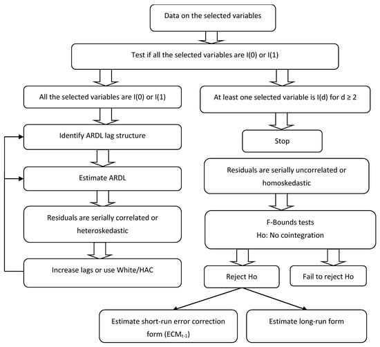
Figure 1.
A flowchart summary of the stationarity tests in Section 3.2 and the cointegration tests in Section 3.3.
3.3. Cointegration Tests
The autoregressive distributive lag (ARDL) bounds tests developed by Pesaran, Shin [75] was used to explore the cointegration for a long-run association between CO2 emissions, energy consumption, economic growth, population density, and export in China. These tests have the following advantages: (1) bounds tests can be conducted with a mixture of I(0) and I(1) processes [76]; (2) the tests comprise a single-equation setup [75]; (3) the ARDL bounds tests decompose error terms, and multicollinearity are eliminated by taking differencing of data [77]; (4) a sufficient number of lags lengths can be assigned, and the automatic lag specification in the ARDL framework is used to remove any multicollinearity and endogeneity problems [78,79].
The ARDL bounds tests were undertaken as follows. The joint F-statistic was used to test the null hypothesis of no cointegration. If the calculated F-statistic was below the lower bound of critical value, the null hypothesis failed to be rejected. If the calculated F-statistic was above the upper bound of critical value, the null hypothesis was rejected. If the calculated F-statistic was between the upper and lower limits of critical value, no conclusion could be made.
The ARDL method included two steps for estimating the long-run relationship. The first step consisted of testing the long-run association amongst all selected variables. If a long-run relationship exists between the variables, the second step was to estimate the long-run model with the least squares, and short-run error correction model. The ARDL long-run and ARDL short-run forms are expressed in Equations (4) and (5), respectively. Model 5 was only valid if the coefficient of lagged error term (ECMt−1) was negative and significant. In addition, ECMt−1 suggests the speed of convergence from short-run towards the long-run equilibrium path (see Figure 1).
We also applied the approach by Johansen [80] and Johansen [81] to test the robustness of ARDL bounds test for the long-run relationship.
3.4. Model Stability and Diagnostic Tests
We used stability tests, including the cumulative sum of recursive residuals (CUSUM) and the cumulative sum of squares of recursive residuals (CUSUMSQ), developed by Brown et al. (1975) [82] and Pesaran and Pesaran (1997). If the CUSUM and CUSUMSQ statistics were within the 5% critical boundaries, the long-run and short-run parameters in our models were stable and could not be rejected. To examine the goodness of fit of our ARDL models, we conducted diagnostic tests, including a normality test, a Heteroskedasticity test, a Breusch–Godfrey Serial Correlation LM test, and a Ramsey RESET.
3.5. Granger Causality Tests
As the ARDL cointegration approach does not explore the direction of causality among CO2 emissions, energy consumption, economic growth, population density, and export, we used the VECM Granger causality tests [83] to examine the direction of causality amongst the selected variables. Granger [83] argued that, with the existence of cointegration, the VECM Granger causality tests are appropriate to explore the long-run and short-run causal relationships between the CO2 emissions, energy consumption, population density, economic growth, and exports (see Figure 2). The VECM model is demonstrated as follows:
where β, a, δ, and γ are coefficients; and ε is white noise.
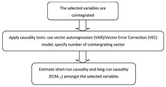
Figure 2.
Shows the approach of the causality tests in Section 3.5.
3.6. Data Sources
The data on CO2 emissions (metric tons) per capita and energy consumption (kg of oil equivalent) per capita were collected from the World Development Indicators [84] and Statistical Review of World Energy [85]. The population density (people per square km of land area), economic growth (GDP per capita at constant 2010 USD), and exports of goods and services per capita (constant 2010 USD) were collected from the World Development Indicators [84]. The data period of the current study is 1971–2018, where annual observations are used.
3.7. Preliminary Examinations of Data
All variables were transformed into natural logarithms. A summary statistic of the variables used in this study is presented in Table 1. Table 1 shows that all the variables have normal distribution, as confirmed by a Jarque–Bera test. The minimum and maximum values of CO2 emissions, economic growth, and exports per capita are noticeable. The lowest value of CO2 emissions is 0.04, the highest value is 1.92; the minimum value of export per capita is 1.89, the maximum value is 7.32; and the minimum value of growth variable is 5.47, while the maximum value is 8.95. Figure 3 indicates the upward trends of the CO2 emissions, energy consumption, GDP per capita, population density, and trade per capita in China from 1971 to 2018. Growth was continuous over the sample period and rose sharply, especially after 1979. A sharp rising trend of energy consumption and CO2 emissions, especially after 2001, was also noticeable.

Table 1.
Descriptive statistics.
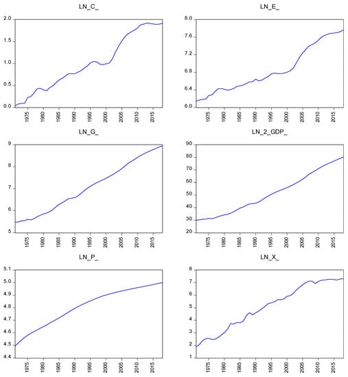
Figure 3.
Trend lines of logarithms of CO2 emissions, energy consumption, GDP per capita, population density, and exports per capita in China from 1971 to 2018. (Source: Authors’ calculations).
4. Findings and Discussions
4.1. The Findings of Unit Root Tests
The results of unit root tests [74] indicate that all the variables of interest show unit root problems at their level, but are found to be integrated at I(1) (see Table 2). Therefore, we applied the ARDL bounds tests to investigate the long-run relationship between CO2 emissions, energy consumption, population density, economic growth, and exports for the period of 1971–2018.
Table 2.
Dickey–Fuller GLS Unit Root Test.
4.2. The Results of Cointegration Tests
As the choice of lag length can affect the F-test, it is necessary to choose the proper lag order of the variables before applying ARDL bounds tests. We chose the automatic selection of lag length for our dependent variable (CO2 emissions) and independent variables (energy consumption, economic growth, population density, and exports).
The results of the ARDL bounds tests [75] for the long-run relationship between the selected variables show that the calculated F-statistic is significant at 5% if CO2 emission is a dependent variable. In addition, the calculated F-statistics are significant at 1% if energy consumption, economic growth, and population density are dependent variables, respectively. The diagnostic tests’ findings demonstrate the validity of the estimation (Table 3). For example, the results of the diagnostic tests show that the model passes all tests, demonstrating no issues with normality, heteroskedasticity, serial correlation, and omitted variables. As the ARDL bounds tests decompose error terms, multicollinearity issues are eliminated by taking the differencing of data [77]. To save space, we report the findings of the ARDL bounds test for CO2 emissions as a dependent variable (Table 3). The findings of the ARDL bounds test for energy consumption, economic growth, population density, and exports, as dependent variables, are made available upon request.
Table 3.
ARDL bounds test for cointegration.
To check the robustness of the ARDL bounds test results, we furthermore used the Johansen’s cointegration tests [81]. The results of the trace test and the maximum eigen value tests [81] (Table 4) are consistent with the findings of the ARDL bounds tests [75]. Hence, we rejected the null hypotheses of no cointegration, and the variables of interest are cointegrated for a long-run relationship.
Table 4.
Results of the Johansen’s cointegration tests.
4.3. The Long-Run and Short-Run Analyses
We investigated the marginal impacts of energy consumption, population density, economic growth, and exports on CO2 emissions. The long-run analyses (Table 5) indicate that energy consumption positively and significantly affects CO2 emissions. For instance, a 1% rise in energy consumption, keeping other factors constant, leads to a 1.35% increase in CO2 emissions. This result is consistent with Balsalobre-Lorente, Shahbaz [37], Ahmed, Bhattacharya [38], Jalil and Mahmud [86], Ang [87], Say and Yücel [88], Halicioglu [56], and Hamilton and Turton [89]. In contrast, a 1% rise in exports is associated with a 0.15 decline in CO2 emissions. The negative sign for exports may be interpreted as demonstrating that China has used more environmentally friendly technologies for its export production. This finding is consistent with Haq, Zhu [59] and Shahbaz, Lean [60], who suggest that exports may decrease CO2 emissions as a result of positive technological effects. In addition, the time trend shows that CO2 emissions declined by 0.04% when there was a 1% increase in technology improvement.
Table 5.
Long-run and short-run analyses.
Of a particular interest is that both linear and nonlinear forms of real GDP show evidence in supporting an inverted-U relationship between economic growth and CO2 emissions. The findings show that, in the long-run, a 1% increase in real GDP raises CO2 emissions by 2.23%, whereas the negative sign of the squared form of real GDP supports the delinking of real GDP and CO2 emissions. The calculated turning point of real GDP per capita was USD 7688, compared to the highest value in our sample of USD 7755 (graphical presentation is made available upon request). These findings are in line with the EKC hypothesis that CO2 emissions rise in the initial period of economic growth and decrease after a threshold point. The findings are in line with Sarkodie and Strezov [90], Jalil and Mahmud [86], Diao, Zeng [91], Riti, Song [92], Rahman and Velayutham [8], Shahbaz, Nasir [10], Zoundi [11], Tao, Zheng [93], He [94], and Fodha and Zaghdoud [95].
The short-run dynamics findings are shown in Table 5. The results indicate that a 1% rise in energy consumption is significantly associated with a 0.4% rise in CO2 emissions; however, the short-run energy consumption elasticity for CO2 emissions (0.4) is much less than the long-run elasticity for CO2 emissions (1.35). The coefficients of real GDP and GDP2 also provide evidence of an inverted-U Kuznets curve in the short-run. In addition, the short-run squared income elasticity for CO2 emissions (in absolute value) is greater than the long-run elasticity for CO2 emissions; this finding further demonstrates the presence of an inverted-U Kuznets curve. The impacts of energy consumption and economic growth (real GDP squared Gt2) in the short-run may be interpreted as indicating that the Chinese government, for the first time in 2007, emphasized the quality rather than the quantity of economic growth [96]. The 2007 Chinese Communist Party Congress called on all sectors, industries, and people in China to change their behaviors to protect the environment [96]. The government also started promoting energy-efficient technologies in the construction and mining sectors, as well as subsidized energy-efficient lighting products and automobiles. It also offered a variety of financial supports and taxes for customers who traded in energy-inefficient products for new, energy-saving ones. In addition, the lower significant positive sign of energy consumption can be explained by the fact that China has recently consumed more renewable energy (short-run). Since 2008, China has issued regulations on renewable energy, water pollution, chemical substances and electronic waste, and emissions and pollution standards [96]. Our finding is consistent with that of Li and Yang [97] who indicated that, to mitigate CO2 emissions, China has developed renewable and nuclear energy resources to substitute for traditional fossil fuels, as well as created energy policies to promote clean energy consumption. Non-fossil energy consumption in China increased from 3.8% in 1965 to 10.9% in 2014. In addition, China plans to raise the share of non-fossil energy in the energy mix to around 20% by 2030. Therefore, the increasing use of renewable energy in recent years may be one of the key factors for the lower energy consumption elasticity for CO2 emissions in China.
The dummy variable (D2002) is significant at 5%. This suggests that CO2 emissions in China increased by 3.3% per year after China joined the WTO in December 2001, although it officially ratified the Kyoto Protocol in August 2002. This may be explained by the fact that China considerably promoted its production for both domestic and foreign markets after it became a member of the WTO [98].
Table 5 shows that the lagged error term (ECMt−1) is −0.28 and statistically significant at 1%. This demonstrates evidence of the long-run relationship between the selected variables. The coefficient indicates that the change in CO2 emissions in China is corrected by 28% per year in the long-run. This implies that the full convergence process may take approximately four years to achieve a stable path of equilibrium, and the adjustment process is fairly fast.
Our results also indicate that, amongst the variables estimated, energy consumption and economic growth (real GDP) are the main factors for CO2 emissions in China in both the short- and long-runs. These findings are consistent with the theory, as expected, and are similar to the findings by Shahbaz, Hye [34], Tang and Tan [40], and Rahman [17]. Surprisingly, the short-run and long-run coefficients of population density are negative; however, they are statistically insignificant. The short-run coefficient of exports is negative but insignificant.
The plots of CUSUM and CUSUMSQ statistics are well within the 5% critical boundaries (Figure 4 and Figure 5), demonstrating that all the long- and short-run parameters in our model are stable.
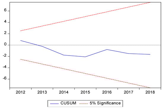
Figure 4.
Plot of cumulative sum of recursive residuals.
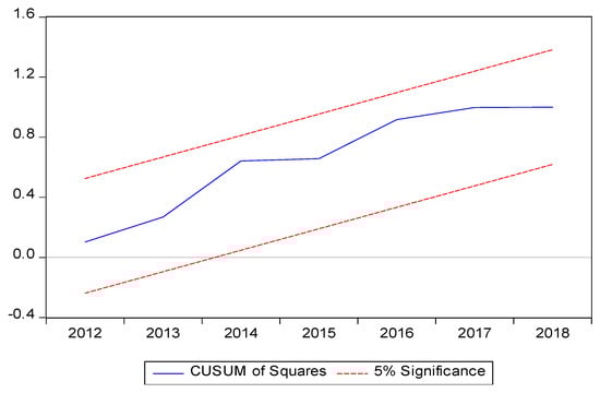
Figure 5.
Plot of cumulative sum of squares of recursive residuals. (Source: Authors’ calculations).
4.4. The VECM Granger Causality Tests
As CO2 emissions, energy consumption, population density, economic growth, and exports in China are cointegrated (see Section 4.2), we undertook the VECM Granger causality tests [83] to investigate the direction of causal relationships between these variables.
The findings shown in Table 6 indicate that short-run unidirectional Granger causality exists from economic growth to CO2 emissions, energy consumption, and exports. In addition, short-run causal relationships are found from CO2 emissions to energy consumption and exports. In regard to long-run causality amongst the selected variables, the coefficients of ECMt−1 in CO2 emissions and exports are significant at 5% and 1%, respectively (Table 6). These findings provide evidence of long-run bidirectional causality relationships between CO2 emissions and exports.
Table 6.
The results of VECM Granger Causality approach.
5. Conclusions and Policy Implications
This paper explores the main factors for environmental degradation in China, and whether the environmental Kuznets curve hypothesis holds in the country over the period of 1971–2018. We apply the unit root tests for the stationarity analyses of selected variables, and the ARDL bounds tests for the long-run links among the variables. The causal relationships amongst CO2 emissions, energy consumption, economic growth, population density, and exports are explored by the VECM Granger causality approach. The obtained results demonstrate that the selected variables are cointegrated. In addition, the energy consumption and economic growth (real GDP) found are the major factors for CO2 emissions in both the short-run and the long-run. In contrast, exports decrease CO2 emissions in the long run. The results also show that the environmental Kuznets curve held in China during the study period of 1971–2018. The results of the VECM causality tests provide evidence of short-run unidirectional Granger causality running from economic growth to CO2 emissions, energy consumption, and exports, as well as from CO2 emissions to energy consumption and exports. Moreover, the long-run causal links are found between CO2 emissions and exports.
Based on our empirical results, the following policy recommendations are worth noting: Firstly, China’s economic growth rate over the last decades is remarkable, which has resulted in high energy consumption, as well as environmental degradation. However, this growth rate will not be sustainable in the long term while maintaining the desired environmental quality. Therefore, China should set a policy target for a reasonable economic growth rate each year, and emphasize the quality rather than the quantity of economic growth. China should limit very high growth aspirations through production which demands excessive use of nonrenewable energy that ultimately increases CO2 emissions. Even if the current annual economic growth rate and energy consumption levels are considered desirable for the sake of the economy, China should explore more green energy sources which are environmentally friendly. Although China’s COVID-19 responses comprise elements of a green recovery, and the Chinese government has announced more comprehensive stimulus packages towards a digital economy [99], the effective implementation of the policies is critical.
Secondly, more imports of energy efficient technologies for domestic production, along with the national carbon credit trading market, should take place sooner to reduce CO2 emissions. In 2017, the Chinese government piloted the emissions trading scheme that incentivizes companies in five cities within Hubei and Guangdong to cut emissions by putting a “price” on CO2 [100]. The pilot achieved some success, with approximately 38 million tons of CO2 traded in regional carbon markets. Although the trading scheme officially in early 2021 [101], the successful implementation of the scheme across the country is important.
Thirdly, the government should encourage and provide incentives for greater use of renewable energy to mitigate CO2 emissions, as well as environmental damage. More than 300 million motor vehicles use less energy efficient engines on the roads in China; they are major sources of CO2 emissions [101]. The government needs to continue the limits on fuel consumption for new motorcycles and mopeds, and suspend car models that do not meet strict fuel standards. The government also needs to further implement incentives to encourage the transition to electric vehicles.
Fourthly, all sectors, industries, and people in China should be further educated through campaigns, advertisements, and training in order to encourage them to change their behavior and require responsibility for environmental protection, as noted by the 2007 Chinese Communist Party Congress. The Chinese government should further cultivate public support for energy conservation and environmental awareness [101].
Finally, rather than focusing on separate individual sectoral policies, a combined policy for sustainable economic growth, energy consumption, environmental protection, and optimum trade, through public and private partnership and initiatives, might be more fruitful. Therefore, future research should be directed to: (i) determine the desired economic growth rate for the short-run, medium, and long-run; (ii) set the target for annual CO2 emissions level; (iii) set the increased proportion of renewable energy consumption compared to nonrenewable energy; and (iv) find out the optimum production, consumption, and trade volume.
Author Contributions
M.M.R.: conceptualization, investigation, literature review, review and editing; X.-B.V.: investigation, literature review, data curation, methodology, formal analysis, writing—original draft, review and editing. All authors have read and agreed to the published version of the manuscript.
Funding
This research received no external funding.
Institutional Review Board Statement
Not applicable.
Informed Consent Statement
Not applicable.
Data Availability Statement
World Development Indicators: https://data.worldbank.org/country/china?view=chart (accessed on 10 January 2020); Statistical Review of World Energy: https://www.bp.com/en/global/corporate/energy-economics/statistical-review-of-world-energy.html (accessed on 15 January 2020).
Conflicts of Interest
The authors declare no conflict of interest.
Abbreviations
| AIC | Akaike information criterion |
| ARDL | Autoregressive Distributed Lag |
| CUSUM | Cumulative sum of recursive residuals |
| CUSUMSQ | Cumulative sum of squares of recursive residuals |
| EKC | Environmental Kuznets Curve |
| GDP | Gross Domestic Product |
| ECM | Lagged error term |
| UN | United Nations |
| VECM | Vector Error Correction Model |
| WTO | World Trade Organisation |
| Ct | CO2 emissions per capita, |
| Et | Energy consumption per capita |
| Gt (Gt2) | Real GDP (squared) per capita |
| Pt | Population density |
| Xt | Export per capita |
| μt | Error term |
References
- World_bank. World Development Indicators. World Bank. 2020. Available online: http://data.worldbank.org/country/china (accessed on 10 January 2020).
- KNOEMA. World Data Atlas. 2020. Available online: https://knoema.com/atlas (accessed on 31 January 2020).
- Conserve_Energy_Future. Overpopulation: Causes, Effects and Solutions. Conserve Energy Future. 2018. Available online: https://www.conserve-energy-future.com/causes-effects-solutions-of-overpopulation.php (accessed on 31 January 2020).
- Michieka, N.M.; Fletcher, J.J.; Burnett, W. An empirical analysis of the role of China’s exports on CO2 emissions. Appl. Energy 2013, 104, 258–267. [Google Scholar] [CrossRef]
- Dinda, S. Environmental Kuznets Curve Hypothesis: A Survey. Ecol. Econ. 2004, 49, 431–455. [Google Scholar] [CrossRef]
- Alam, M.; Murad, W.; Noman, A.H.M.; Ozturk, I. Relationships among carbon emissions, economic growth, energy consumption and population growth: Testing Environmental Kuznets Curve hypothesis for Brazil, China, India and Indonesia. Ecol. Indic. 2016, 70, 466–479. [Google Scholar] [CrossRef]
- Sarkodie, S.A.; Ozturk, I. Investigating the Environmental Kuznets Curve hypothesis in Kenya: A multivariate analysis. Renew. Sustain. Energy Rev. 2020, 117, 109481. [Google Scholar] [CrossRef]
- Rahman, M.M.; Velayutham, E. Renewable and non-renewable energy consumption-economic growth nexus: New evidence from South Asia. Renew. Energy 2020, 147, 399–408. [Google Scholar] [CrossRef]
- Rahman, A.; Murad, S.M.W.; Ahmad, F.; Wang, X. Evaluating the EKC Hypothesis for the BCIM-EC Member Countries under the Belt and Road Initiative. Sustainability 2020, 12, 1478. [Google Scholar] [CrossRef]
- Shahbaz, M.; Nasir, M.A.; Roubaud, D. Environmental degradation in France: The effects of FDI, financial development, and energy innovations. Energy Econ. 2018, 74, 843–857. [Google Scholar] [CrossRef]
- Zoundi, Z. CO2 emissions, renewable energy and the Environmental Kuznets Curve, a panel cointegration approach. Renew. Sustain. Energy Rev. 2017, 72, 1067–1075. [Google Scholar] [CrossRef]
- Lean, H.H.; Smyth, R. CO2 emissions, electricity consumption and output in ASEAN. Appl. Energy 2010, 87, 1858–1864. [Google Scholar] [CrossRef]
- Tiwari, A.K.; Shahbaz, M.; Hye, Q.M.A. The environmental Kuznets curve and the role of coal consumption in India: Cointegration and causality analysis in an open economy. Renew. Sustain. Energy Rev. 2013, 18, 519–527. [Google Scholar] [CrossRef]
- Ertugrul, H.M.; Cetin, M.; Seker, F.; Dogan, E. The impact of trade openness on global carbon dioxide emissions: Evidence from the top ten emitters among developing countries. Ecol. Indic. 2016, 67, 543–555. [Google Scholar] [CrossRef]
- Kanjilal, K.; Ghosh, S. Environmental Kuznet’s curve for India: Evidence from tests for cointegration with unknown structuralbreaks. Energy Policy 2013, 56, 509–515. [Google Scholar] [CrossRef]
- Sephton, P.; Mann, J. Further evidence of an Environmental Kuznets Curve in Spain. Energy Econ. 2013, 36, 177–181. [Google Scholar] [CrossRef]
- Rahman, M.M. Do population density, economic growth, energy use and exports adversely affect environmental quality in Asian populous countries? Renew. Sustain. Energy Rev. 2017, 77, 506–514. [Google Scholar] [CrossRef]
- Arouri, M.E.H.; Ben Youssef, A.; M’Henni, H.; Rault, C. Energy consumption, economic growth and CO2 emissions in Middle East and North African countries. Energy Policy 2012, 45, 342–349. [Google Scholar] [CrossRef]
- Ozturk, I.; Acaravci, A. CO2 emissions, energy consumption and economic growth in Turkey. Renew. Sustain. Energy Rev. 2010, 14, 3220–3225. [Google Scholar] [CrossRef]
- Musolesi, A.; Mazzanti, M.; Zoboli, R. A panel data heterogeneous Bayesian estimation of environmental Kuznets curves for CO2 emissions. Appl. Econ. 2010, 42, 2275–2287. [Google Scholar] [CrossRef]
- Pao, H.-T.; Yu, H.-C.; YANG, Y.-H. Modeling the CO2 emissions, energy use, and economic growth in Russia. Energy 2011, 36, 5094–5100. [Google Scholar] [CrossRef]
- He, J.; Richard, P. Environmental Kuznets curve for CO2 in Canada. Ecol. Econ. 2010, 69, 1083–1093. [Google Scholar] [CrossRef]
- Tunç, G.I.; Türüt-Aşık, S.; Akbostancı, E. A decomposition analysis of CO2 emissions from energy use: Turkish case. Energy Policy 2009, 37, 4689–4699. [Google Scholar] [CrossRef]
- Kashem, M.A.; Rahman, M.M. CO2 Emissions and Development Indicators: A Causality Analysis for Bangladesh. Environ. Process. 2019, 6, 433–455. [Google Scholar] [CrossRef]
- Alam, M.J.; Begum, I.A.; Buysse, J.; Rahman, S.; Van Huylenbroeck, G. Dynamic modeling of causal relationship between energy consumption, CO2 emissions and economic growth in India. Renew. Sustain. Energy Rev. 2011, 15, 3243–3251. [Google Scholar] [CrossRef]
- Appiah, M.O. Investigating the multivariate Granger causality between energy consumption, economic growth and CO2 emissions in Ghana. Energy Policy 2018, 112, 198–208. [Google Scholar] [CrossRef]
- Alam, M.J.; Begum, I.A.; Buysse, J.; Van Huylenbroeck, G. Energy consumption, carbon emissions and economic growth nexus in Bangladesh: Cointegration and dynamic causality analysis. Energy Policy 2012, 45, 217–225. [Google Scholar] [CrossRef]
- Koengkan, M.; Losekann, L.D.; Fuinhas, J.A. The relationship between economic growth, consumption of energy, and environmental degradation: Renewed evidence from Andean community nations. Environ. Syst. Decis. 2018, 39, 95–107. [Google Scholar] [CrossRef]
- Koengkan, M.; Fuinhas, J.A.; Santiago, R. The relationship between CO2 emissions, renewable and non-renewable energy consumption, economic growth, and urbanisation in the Southern Common Market. J. Environ. Econ. Policy 2020, 9, 1–19. [Google Scholar] [CrossRef]
- Rahman, M.M.; Kashem, M.A. Carbon emissions, energy consumption and industrial growth in Bangladesh: Empirical evidence from ARDL cointegration and Granger causality analysis. Energy Policy 2017, 110, 600–608. [Google Scholar] [CrossRef]
- Khan, M.K.; Rehan, M. The relationship between energy consumption, economic growth and carbon dioxide emissions in Pakistan. Financ. Innov. 2020, 6, 1–13. [Google Scholar] [CrossRef]
- Uddin, G.S.; Bidisha, S.H.; Ozturk, I. Carbon emissions, energy consumption, and economic growth relationship in Sri Lanka. Energy Sources Part B Econ. Plan. Policy 2016, 11, 282–287. [Google Scholar] [CrossRef]
- Kasman, A.; Duman, Y.S. CO2 emissions, economic growth, energy consumption, trade and urbanization in new EU member and candidate countries: A panel data analysis. Econ. Model. 2015, 44, 97–103. [Google Scholar] [CrossRef]
- Shahbaz, M.; Hye, Q.M.A.; Tiwari, A.K.; Leitão, N.C. Economic growth, energy consumption, financial development, international trade and CO2 emissions in Indonesia. Renew. Sustain. Energy Rev. 2013, 25, 109–121. [Google Scholar] [CrossRef]
- Hossain, S. An Econometric Analysis for CO2 Emissions, Energy Consumption, Economic Growth, Foreign Trade and Urbanization of Japan. Low Carbon Econ. 2012, 3, 92–105. [Google Scholar] [CrossRef]
- Adedoyin, F.F.; Zakari, A. Energy consumption, economic expansion, and CO2 emission in the UK: The role of economic policy uncertainty. Sci. Total Environ. 2020, 738, 140014. [Google Scholar] [CrossRef]
- Balsalobre-Lorente, D.; Shahbaz, M.; Roubaud, D.; Farhani, S. How economic growth, renewable electricity and natural resources contribute to CO2 emissions? Energy Policy 2018, 113, 356–367. [Google Scholar] [CrossRef]
- Ahmed, K.; Bhattacharya, M.; Shaikh, Z.; Ramzan, M.; Ozturk, I. Emission intensive growth and trade in the era of the Association of Southeast Asian Nations (ASEAN) integration: An empirical investigation from ASEAN-8. J. Clean. Prod. 2017, 154, 530–540. [Google Scholar] [CrossRef]
- Begum, R.A.; Sohag, K.; Abdullah, S.M.S.; Jaafar, M. CO2 emissions, energy consumption, economic and population growth in Malaysia. Renew. Sustain. Energy Rev. 2015, 41, 594–601. [Google Scholar] [CrossRef]
- Tang, C.F.; Tan, B.W. The impact of energy consumption, income and foreign direct investment on carbon dioxide emissions in Vietnam. Energy 2015, 79, 447–454. [Google Scholar] [CrossRef]
- Ben Mbarek, M.; Saidi, K.; Rahman, M.M. Renewable and non-renewable energy consumption, environmental degradation and economic growth in Tunisia. Qual. Quant. 2018, 52, 1105–1119. [Google Scholar] [CrossRef]
- Soytas, U.; Sari, R.; Ewing, B.T. Energy consumption, income, and carbon emissions in the United States. Ecol. Econ. 2007, 62, 482–489. [Google Scholar] [CrossRef]
- Engelman, R. Profiles in Carbon: An Update on Population, Consumption, and Carbon Dioxide Emissions; Population Action International: Washington, DC, USA, 1998. [Google Scholar]
- O’Neill, B.C.; Mackellar, F.L.; Lutz, W.; Macdonald, G. Population and Climate Change; Cambridge University Press (CUP): Cambridge, UK, 2000. [Google Scholar]
- Mamun, A.; Sohag, K.; Mia, A.H.; Uddin, G.S.; Ozturk, I. Regional differences in the dynamic linkage between CO2 emissions, sectoral output and economic growth. Renew. Sustain. Energy Rev. 2014, 38, 1–11. [Google Scholar] [CrossRef]
- Ohlan, R.P. The impact of population density, energy consumption, economic growth and trade openness on CO2 emissions in India. Nat. Hazards 2015, 79, 1409–1428. [Google Scholar] [CrossRef]
- Chen, J.; Wang, B.; Huang, S.; Song, M. The influence of increased population density in China on air pollution. Sci. Total Environ. 2020, 735, 139456. [Google Scholar] [CrossRef] [PubMed]
- Rahman, M.M.; Saidi, K.; Ben Mbarek, M. Economic growth in South Asia: The role of CO2 emissions, population density and trade openness. Heliyon 2020, 6, e03903. [Google Scholar] [CrossRef]
- Shi, A. Population growth and global carbon dioxide emissions. In Proceedings of the IUSSP Conference in Brazil/session-s09, Bahia, Brazil, 18–24 August 2001. [Google Scholar]
- Rahman, M.M.; Vu, X.-B. The nexus between renewable energy, economic growth, trade, urbanisation and environmental quality: A comparative study for Australia and Canada. Renew. Energy 2020, 155, 617–627. [Google Scholar] [CrossRef]
- Schmalensee, R.; Stoker, T.M.; Judson, R.A. World carbon dioxide emissions: 1950–2050. Rev. Econ. Stat. 1998, 80, 15–27. [Google Scholar] [CrossRef]
- Jebli, M.B.; Youssef, S.B.; Apergis, N. The dynamic linkage between renewable energy, tourism, CO 2 emissions, economic growth, foreign direct investment, and trade. Lat. Am. Econ. Rev. 2019, 28, 2. [Google Scholar] [CrossRef]
- Gasimli, O.; Haq, I.U.; Gamage, S.K.N.; Shihadeh, F.; Rajapakshe, P.S.K.; Shafiq, M. Energy, Trade, Urbanization and Environmental Degradation Nexus in Sri Lanka: Bounds Testing Approach. Energies 2019, 12, 1655. [Google Scholar] [CrossRef]
- Mahmood, H.; Maalel, N.; Zarrad, O. Trade Openness and CO2 Emissions: Evidence from Tunisia. Sustainability 2019, 11, 3295. [Google Scholar] [CrossRef]
- Murad, M.W.; Mazumder, M.N.H. Trade and environment: Review of relationship and implication of environmental Kuznets curve hypothesis for Malaysia. J. Soc. Sci. 2009, 19, 83–90. [Google Scholar] [CrossRef]
- Halicioglu, F. An econometric study of CO2 emissions, energy consumption, income and foreign trade in Turkey. Energy Policy 2009, 37, 1156–1164. [Google Scholar] [CrossRef]
- Khan, Z.; Ali, M.; Jinyu, L.; Shahbaz, M.; Siqun, Y. Consumption-based carbon emissions and trade nexus: Evidence from nine oil exporting countries. Energy Econ. 2020, 89, 104806. [Google Scholar] [CrossRef]
- Muhammad, S.; Long, X.; Salman, M.; Dauda, L. Effect of urbanization and international trade on CO2 emissions across 65 belt and road initiative countries. Energy 2020, 196, 117102. [Google Scholar] [CrossRef]
- Haq, I.U.; Zhu, S.; Shafiq, M. Empirical investigation of environmental Kuznets curve for carbon emission in Morocco. Ecol. Indic. 2016, 67, 491–496. [Google Scholar] [CrossRef]
- Shahbaz, M.; Lean, H.H.; Shabbir, M.S. Environmental Kuznets Curve hypothesis in Pakistan: Cointegration and Granger causality. Renew. Sustain. Energy Rev. 2012, 16, 2947–2953. [Google Scholar] [CrossRef]
- Rahman, M.M.; Saidi, K.; Mbarek, M.B. The effects of population growth, environmental quality and trade openness on economic growth: A panel data application. J. Econ. Stud. 2017, 44, 456–474. [Google Scholar] [CrossRef]
- Haug, A.A.; Ucal, M. The role of trade and FDI for CO2 emissions in Turkey: Nonlinear relationships. Energy Econ. 2019, 81, 297–307. [Google Scholar] [CrossRef]
- Hasanov, F.J.; Liddle, B.; Mikayilov, J.I. The impact of international trade on CO2 emissions in oil exporting countries: Territory vs consumption emissions accounting. Energy Econ. 2018, 74, 343–350. [Google Scholar] [CrossRef]
- Jalil, A.; Feridun, M. The impact of growth, energy and financial development on the environment in China: A cointegration analysis. Energy Econ. 2011, 33, 284–291. [Google Scholar] [CrossRef]
- Kuznets, S. Economic Growth and Income Inequality. Am. Econ. Rev. 1955, 45, 1–28. [Google Scholar]
- Saidi, K.; Hammami, S. The effect of energy consumption and economic growth on CO2 emissions: Evidence from 58 countries. Bull. Energy Econ. Bee 2015, 3, 91–104. [Google Scholar]
- Benjamin, D. Is free trade good for the environment? Perc. Rep. 2002, 20. Available online: https://www.perc.org/2002/03/01/is-free-trade-good-for-the-environment/ (accessed on 20 June 2020).
- OECD. Trade and Environment. Organisation for Economic Co-operation and Development. 2018. Available online: https://www.oecd.org/trade/topics/trade-and-the-environment/ (accessed on 20 June 2020).
- Antweiler, W.; Copeland, B.R.; Taylor, M.S. Is Free Trade Good for the Environment? Am. Econ. Rev. 2001, 91, 877–908. [Google Scholar] [CrossRef]
- Xu, M.; Li, R.; Crittenden, J.C.; Chen, Y. CO2 emissions embodied in China’s exports from 2002 to 2008: A structural decomposition analysis. Energy Policy 2011, 39, 7381–7388. [Google Scholar] [CrossRef]
- WTO. China and the WTO. World Trade Organization. 2019. Available online: https://www.wto.org/english/thewto_e/countries_e/china_e.htm (accessed on 20 June 2020).
- UN. Kyoto Protocol: China’s Ratification status. United Nations Climate Change. 2019. Available online: https://unfccc.int/node/180417 (accessed on 20 June 2020).
- Dickey, D.A.; Fuller, W.A. Distribution of the estimators for autoregressive time series with a unit root. J. Am. Stat. Assoc. 1979, 74, 427–431. [Google Scholar]
- Elliott, G.; Rothenberg, T.J.; Stock, J.H. Efficient Tests for an Autoregressive Unit Root. Econometrica 1996, 64, 813. [Google Scholar] [CrossRef]
- Pesaran, M.H.; Shin, Y.; Smithc, R.J. Bounds testing approaches to the analysis of level relationships. J. Appl. Econ. 2001, 16, 289–326. [Google Scholar] [CrossRef]
- Pesaran, M.H.; Pesaran, B. Working with Microfit 4.0: Interactive Econometric Analysis; Oxford University Press: Oxford, UK, 1997. [Google Scholar]
- Shabbir, A.H.; Zhang, J.; Liu, X.; Lutz, J.A.; Valencia, C.; Johnston, J.D. Determining the sensitivity of grassland area burned to climate variation in Xilingol, China, with an autoregressive distributed lag approach. Int. J. Wildland Fire 2019, 28, 628. [Google Scholar] [CrossRef]
- Pesaran, M.H.; Shin, Y. An autoregressive distributed-lag modelling approach to cointegration analysis. Econom. Soc. Monogr. 1998, 31, 371–413. [Google Scholar]
- Brown, S.P.; McDonough, I.K. Using the Environmental Kuznets Curve to evaluate energy policy: Some practical considerations. Energy Policy 2016, 98, 453–458. [Google Scholar] [CrossRef]
- Johansen, S. Statistical analysis of cointegration vectors. J. Econ. Dyn. Control 1988, 12, 231–254. [Google Scholar] [CrossRef]
- Johansen, S. Estimation and hypothesis testing of cointegration vectors in Gaussian vector. Econometrica 1991, 59, 1551–1580. [Google Scholar] [CrossRef]
- Brown, R.L.; Durbin, J.; Evans, J.M. Techniques for Testing the Constancy of Regression Relationships over Time. J. R. Stat. Soc. Ser. B Stat. Methodol. 1975, 37, 149–163. [Google Scholar] [CrossRef]
- Granger, C.W.J. Investigating Causal Relations by Econometric Models and Cross-spectral Methods. Econometrica 1969, 37, 424. [Google Scholar] [CrossRef]
- WDI. World Development Indicators. 2019. Available online: https://data.worldbank.org/indicator/EG.FEC.RNEW.ZS (accessed on 10 January 2020).
- BP. BP Statistical Review of World Energy. 2019. Available online: https://www.bp.com/content/dam/bp/business-sites/en/global/corporate/pdfs/energy-economics/statistical-review/bp-stats-review-2019-full-report.pdf (accessed on 15 January 2020).
- Jalil, A.; Mahmud, S.F. Environment Kuznets curve for CO2 emissions: A cointegration analysis for China. Energy Policy 2009, 37, 5167–5172. [Google Scholar] [CrossRef]
- Ang, J.B. CO2 emissions, energy consumption, and output in France. Energy Policy 2007, 35, 4772–4778. [Google Scholar] [CrossRef]
- Say, N.P.; Yücel, M. Energy consumption and CO2 emissions in Turkey: Empirical analysis and future projection based on an economic growth. Energy Policy 2006, 34, 3870–3876. [Google Scholar] [CrossRef]
- Hamilton, C.; Turton, H. Determinants of emissions growth in OECD countries. Energy Policy 2002, 30, 63–71. [Google Scholar] [CrossRef]
- Sarkodie, S.A.; Strezov, V. A review on Environmental Kuznets Curve hypothesis using bibliometric and meta-analysis. Sci. Total Environ. 2019, 649, 128–145. [Google Scholar] [CrossRef]
- Diao, X.; Zeng, S.; Tam, C.; Tam, V.W. EKC analysis for studying economic growth and environmental quality: A case study in China. J. Clean. Prod. 2009, 17, 541–548. [Google Scholar] [CrossRef]
- Riti, J.S.; Song, D.; Shu, Y.; Kamah, M. Decoupling CO2 emission and economic growth in China: Is there consistency in estimation results in analyzing environmental Kuznets curve? J. Clean. Prod. 2017, 166, 1448–1461. [Google Scholar] [CrossRef]
- Tao, S.; Zheng, T.; Lianjun, T. An empirical test of the environmental Kuznets curve in China: A panel cointegration approach. China Econ. Rev. 2008, 19, 381–392. [Google Scholar]
- He, J. China’s industrial SO2 emissions and its economic determinants: EKC’s reduced vs. structural model and the role of international trade. Environ. Dev. Econ. 2009, 14, 227–262. [Google Scholar] [CrossRef]
- Fodha, M.; Zaghdoud, O. Economic growth and pollutant emissions in Tunisia: An empirical analysis of the environmental Kuznets curve. Energy Policy 2010, 38, 1150–1156. [Google Scholar] [CrossRef]
- Kan, J. Environmentally Friendly Consumers Emerge. China Business Review. 2010. Available online: https://www.chinabusinessreview.com/environmentally-friendly-consumers-emerge/ (accessed on 25 January 2020).
- Li, D.; Yang, D. Does Non-Fossil Energy Usage Lower CO2 Emissions? Empirical Evidence from China. Sustainability 2016, 8, 874. [Google Scholar] [CrossRef]
- STATISTA. Teritorial Carbon Dioxide Emissions in China from 2001 to 2017. 2019. Available online: https://www.statista.com/statistics/239093/co2-emissions-in-china/ (accessed on 10 March 2020).
- Climate-Action-Tracker. Climate Action Tracker-Country Summary-China. 2021. Available online: https://climateactiontracker.org/countries/china/ (accessed on 15 March 2021).
- Power, C. How is China Managing Its Greenhouse Gas Emissions. 2020. Available online: https://chinapower.csis.org/china-greenhouse-gas-emissions/ (accessed on 15 March 2021).
- Slater, H.; Shu, W.; Boer, D.D. China Dialogue. China’s National Carbon Market is about to Launch. 2021. Available online: https://chinadialogue.net/en/climate/chinas-national-carbon-market-is-about-to-launch/ (accessed on 15 March 2021).


Publisher’s Note: MDPI stays neutral with regard to jurisdictional claims in published maps and institutional affiliations. |
© 2021 by the authors. Licensee MDPI, Basel, Switzerland. This article is an open access article distributed under the terms and conditions of the Creative Commons Attribution (CC BY) license (http://creativecommons.org/licenses/by/4.0/).