Abstract
The intermittent nature of wind power is a major challenge for wind as an energy source. Wind power generation is therefore difficult to plan, manage, sustain, and track during the year due to different weather conditions. The uncertainty of energy loads and power generation from wind energy sources heavily affects the system stability. The battery energy storage system (BESS) plays a fundamental role in controlling and improving the efficiency of renewable energy sources. Stochasticity of wind speed and reliability of the main system components are considered. This paper presents a dynamical control system based on model predictive control (MPC) in real time, to make full use of the flexibility and controllability of energy storage to mitigate problems of wind farm variability and intermittency. The control scheme first plans the expected output, then stochastic optimization is used to optimize grid integrated wind farm BESS output power, develop an optimal operation strategy for BESS, and prevent some unpredictable conditions that may have impacts on the stability of the system. The results show that the proposed method can reduce grid-connected wind power fluctuations, limit system faults, control command for the BESS in the dispatching period, and ensure system stability for grid connection.
1. Introduction
Electrical energy is a valuable basic human need and, at the same time, a significant source of operation in corporate industries, agriculture, organizations, activities, machinery, residences, etc. [1]. There has been a rise in demand for electrical energy, which has forced the world to explore other alternative energy sources to meet demand, in addition to conventional energy sources such as coal and gas [2]. Renewable Energy Sources (RESs) such as Wind and Solar renewable energy sources have had substantial growth in recent years, with large-scale production underway globally [2].
The Department of Energy (DOE) launched an Integrated Resource Plan (IRP) for South Africa in collaboration with Government, Industry, Labour, Civil Society, and Eskom to plan the implementation of a 17,800 MW renewable energy growth plan to be implemented by 2030 [3]. Forecast studies were performed in line with the IRP and, in 2017, Eskom released a study outlining the need for up to 2 GW of additional, regular balanced energy storage within the current grid [4].
The incorporation of RESs into the grid does not provide a constant supply of electricity, because the output and input of RESs are variable and thus present some technical challenges to the power system. Energy storage systems have been considered as a solution for storing and alleviating energy system challenges, subject to the comparison of various energy storage technologies and supplier products under South African environmental conditions, and to the identification of which products are appropriate for potential energy storage needs of independent power producers (IPPs) and Eskom [4,5].
The literature reviewed confirmed that grid connected wind farms can cause fluctuations and reactive power redistribution, which can lead to frequency fluctuation and voltage imbalance at times. The grid stability and safety are therefore seriously threatened. The power system integrated with a renewable wind farm must be dynamically controlled for system stability and safe operation. Recent developments in storage technology offer an incentive for the use of renewable energies (RES) energy storage systems [6,7,8,9]. For more than a century, conventional energy storage technologies have existed, including pumped or reservoir-based hydro-electric facilities and lead-acid batteries. The past decade has been marked by an increasing interest in both conventional and advanced technologies for energy storage. Advanced batteries (e.g., flow, lithium ion, sodium–sulfur battery (NAS)), new mechanical systems based on compressed air and flywheels, and storage technologies based on thermal and gas (i.e., hydrogen and methane) have been given attention [10]. In Flexible Alternating Current Transmission Systems (FACTS) applications, Large Battery Energy Storage Systems (BESS) are increasingly being used to improve the system’s voltage, frequency, oscillatory, and/or transient stability and thus improve power supply reliability. Two parts consist of a battery energy storage system (BESS). First, a storage component that in an electrochemical process can store/restore energy. Secondly, a rectifier/inverter that can transform the DC voltage required for the grid from the storage component to the AC voltage and vice versa. The rectifier/inverter is normally based on a pulse width modulation (PWM) voltage-sourced converter (VSC). The problem with batteries is the vast variety of technologies and the diversity within one technology as well. So, no simple, precise model is available, valid for all batteries. With battery models, there are two principal challenges. The first issue is to get a model that is not too complex but sufficiently accurate. The second problem is to obtain from manufacturers the parameters or own measurements required for the model. Only a model with suitable parameters can deliver good results. Lead-acid batteries are often common batteries in the industry. But many other types are also available, such as nickel cadmium (NiCd), sodium–sulfur NAS, nickel-metal hybrid (NiMH), and several types of lithium-ion. Each form has its own assets and disadvantages [10,11,12,13,14,15].
At present, the main methods for dealing with uncertainty issues are stochastic optimization, fuzzy optimization and robust optimization [16,17]. Fuzzy optimization usually depends on human experience. Robust optimization is more widely used in line with the actual phenomenon. Stochastic optimization does not depend on human experience nor with the actual phenomenon, but it describes uncertain parameters as discrete or continuous functions of probability density [16]. Stochastic optimization requires the distribution of the probability of unknown parameters and has been widely employed to deal with uncertainties in some areas of, (1) power system planning, (2) comprehensive stochastic optimization model for optimizing the electric power system of wind farms, (3) the investment of components, (4) the system efficiency, and (5) the system reliability such as power transmission planning and capacity expansion planning [18]. For example, [19] investigated stochastic optimization for integration of renewable energy technologies in district energy systems for cost-effective use and discovered uncertainty of energy loads and power generation from renewable energy resources heavily affects the operating cost. In these studies [20,21,22], a two-stage stochastic programming approach to optimal design of distributed energy systems. Thus, this paper proposes a stochastic model for optimizing the wind farm battery energy storage system, by considering network future components planning, the system efficiency, and the system reliability.
The wind energy’s inherently variable nature can cause frequency and voltage fluctuations. The BESS allows these variations to be smoothed out to stabilize the system [15]. Therefore, the BESS output power must be quickly regulated such that excess energy is consumed during output spikes and energy is released during output decreases [23]. For the smoothing function, the ramping capacity is therefore very necessary [24]. The production smoothing in the plant decreases the demand for electricity quality and system auxiliary services [25]. Wind resources are often far from the available high-capacity transmission lines in rural areas. The energy generated cannot be transferred to the load due to the transmission constraints. Further BESS can provide relief for transmission and distribution of congestion, and energy shifts and investment capacity deferral [26,27]. In high and medium voltage grids, wind turbines must also be enabled to engage in static and dynamic grid support. The slow changes in voltage can be preserved to tolerable limits by supplying reactive power conditions with a static frequency stability in normal operations. Nevertheless, because the wind farm input and output are not constant, the integration of the storage system may pose technical challenges to the control system. When the rate of change is large, the systems are said to be dynamic systems [19,28]. Dynamic management of interconnected grid-connected wind farm storage systems would therefore be necessary to ensure the mitigation of variable wind farm output variability and to maintain grid power stability [29]. Based on the state of charge (SOC) of the BESS authors proposed an algorithm for dynamic programming (DP) in order to smoothly fluctuate wind power [30]. Different application of MPC strategies have been applied for wind farm active power control, voltage control, and frequency control. In [31], the hierarchical model predictive control (HMPC) method of wind farm BESS for frequency regulation during black-start (BS) is proposed, which consists of two control modes: frequency regulation mode and reserve recovery mode; The study of [32], provides a novel model prediction control (MPC) based control strategy for BESS, is presented aiming to minimize the equivalent operating cost of BESS during each control step. The study of [33], provides a comprehensive review of model predictive control (MPC) in individual and interconnected microgrids, including both converter-level and grid level control strategies applied to three layers of the hierarchical control architecture. The study of [34] looked at fault effects due to common power-loss malfunctions in solar photovoltaic arrays in the presence of microgrid uncertainties and disturbances. In the [35] study, a model predictive control strategy (with a 24-h prediction horizon) is proposed to reduce the operational cost of microgrids. Nozal, A.R.; et al [31,35,36] achieved a smoothing goal to reduce the action of the BESS using Model Predictive Control (MPC) to ensure the overall results were smooth. In short, the common purpose of the above control algorithms is to reduce the output of wind farms to a large extent. In the areas of renewable energy production and control, MPC is the most widely used of all advanced control methodologies in industrial applications [30].
The preliminary development of this study for accounting for uncertainties in wind energy was previously reported in two references [19,37], which is limited to a multi-period optimal power flow (MPOPF) [19] and robust energy scheduling strategy for intelligent demand-side management (DSM) respectively [37]. A linear wind farm model that includes a dynamic turbine model with time-varying axial induction factors, yaw misalignments, and wake characteristics is presented in [21], with promising results. Another application of a linear model predictive control approach is shown in [22], where the aim is to minimize the wind turbine mechanical loads using a dynamic, linear wind farm flow and operation model. The present article extends this work by the following additional contributions: (1) a model of nonlinear dynamic control for mitigating uncertainties in wind farm battery energy storage system; (2) battery type is considered as means for mitigating challenges introduced by the integration of intermittency and variable wind farm, and; (3) a more complete and structured model control for dynamic wind farm battery energy storage system. Finally, we also include (4) a new case study based on a real South African network system and wind energy production data for simulation cases of battery load flow, outages, and load changes. This research aims to investigate dynamic control model of an integrated wind farm battery energy storage for grid connection in South Africa.
The main novelties of this study are:
- Identify a suitable dynamic control system model and choose battery type for a South African Grid connected Wind Farm BESS,
- Modelling of an integrated wind farm battery energy storage model for grid connection, and
- Conduct a simulation to investigate the effects and impacts of integrated wind farm battery energy storage for grid connection.
The remainder of the journal article is organized as follows: the proposed method is provided in Section 2, the study cases, battery selection type and network simulation are provided in Section 3, the results and discussions are given in Section 4, and the journal conclusions are drawn in Section 5.
2. The Proposed Method
2.1. System Discription
Wind energy is a clean, free, and readily available renewable energy source [38]. It is difficult to plan, manage, sustain, and track wind generation because of its intermittent nature [39]. The fluctuation of wind power should be smoothed while it is dispatched to the grid power to avoid system faults [30]. This paper aims at developing a control system based on model predictive control (MPC) combined with a battery energy storage system (BESS) capable of mitigating problems of wind power variability and intermittency. The overall structure of the integrated Wind Farm Battery Energy Storage System (BESS) is illustrated in Figure 1. The system consists of a wind farm, a BESS, a converter, a Power Management Unit (PMU), and the transmission line connects the system to the main grid. Often the PCC coincides with the POC [40]. Also, this study PCC and POC coincides. At PCC, the BESS is linked to the grid and charges/discharges power through the converter to smooth the wind power injected into the grid. PG(t): Grid-connected power at time t, PW(t): Wind farm output power at t, PB(t): Output power of energy storage battery, SOE: state of the energy, and PMU: Power management unit. A key component of the design of the wind storage system is the BESS PMU used for smoothing the wind power grid [41].
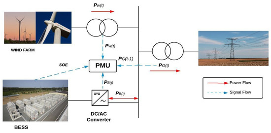
Figure 1.
Structure chart of Grid integrated Wind Farm BESS.
2.2. Control System Modelling
The study considered the battery to be a nonlinear model. A schematic diagram of the whole system is shown in Figure 2. The difference between fluctuated wind power (Pw) and smoothed dispatched power (Pg) will be compensated with battery energy storage (Pc).
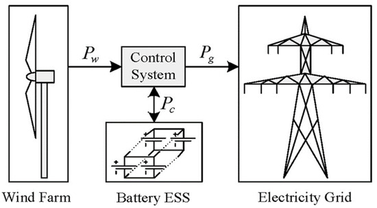
Figure 2.
Wind farm battery Energy Storage System connected to the Grid [14].
The proposed control system blocked diagram is shown in Figure 3. MPC is based on an online optimal control problem solution where a receding horizon approach is used in such a way that an open loop optimal control problem is solved over some future interval for any current state x(k) at time k, taking into account the current and future constraints. The MPC algorithm calculates an open loop sequence of the manipulated variables in a way that optimizes the plant’s future behavior. We then insert into the plant the first value of the optimization. This procedure is repeated using the current state x(k + 1) at the time (k + 1) [42].
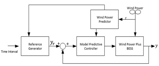
Figure 3.
Proposed control system block diagram [14].
There are two main components to the proposed control system: active reference generator block and controller block based on MPC. This controller is a new insight into the wind farm power control issue, integrated with the device BESS by using this real-time reference generator in the design of the proposed control system [15,43].
The benefits of the control system proposed are the following:
- Optimization in real time and physical limitations of device overall behavior with MPC,
- Updating the reference signal according to machine states and forecast price and wind power estimates, and
- Increased management of the electricity market with the BESS wind farms while retaining the power signal ramp inside predefined barriers.
It has also been seen that the performance of the battery has greatly affected the wind farm. Selecting a suitable battery will enable to fulfil all performance requirements of a wind farm.
2.3. BESS Model
2.3.1. Generic BESS Model
A simple and applicable model, although comprehensive, is one of the important issues in the modelling of renewable energy plants. Battery energy storage is a key component of a wind power plant, although a practical model makes it easier for a control designer to control and optimize the real plant’s performance. Since the battery’s real behavior is nonlinear and we are searching for a model that shows this way, in the state space form, a nonlinear BESS model is defined as follows: [14]:
where x1 or Pg(k) are the power sent to a grid in Figure 1, x2(k) is the battery capacity at phase k, r(k) the unregulated wind power output, u(k) or Pc the power control signal is a positive (u(k) ≥ 0) signal and the battery is charged and discharged respectively for negative u(k) values. Td is a MWh conversion factor. Functions f and g are described in Equations (3) and (4) as representing the battery’s nonlinear behavior:
and:
with these limits:
where x1 or Pg(k) are the power sent to a grid in Figure 1, x2(k) is the battery capacity at phase k, r(k) the unregulated wind power output, u(k) or pc the power control signal is a positive (u(k) ≥ 0) signal, and the battery is charged and discharged respectively for negative u(k) values. Td is a MWh conversion factor. Functions f and g are described in Equations (3) and (4) as representing the battery’s nonlinear behavior: Functions f and g are presented to respond to the actual battery activity during the charge or discharge and storage time, based on Equations (3)–(5). The chart of the proposed control system is shown in Figure 2. The α coefficient is loaded on the battery. In Equation (4), g also means the charge and discharge process when the power signal u(k) is sent to the battery. Due to derived experimental data from a battery type, parameters (α, β and μ) are calculated. In this analysis both α, β and α for simplicity are constant for all x. In relation to the introduction, the novelty of this work is twofold, whether dynamic control of integrated wind farm battery energy storage systems:
f(x) = α (x)x
- Mitigate fluctuations of wind farm variable output, and
- Maintain power stability for grid connection?
The model proposed is an additional battery model that covers energy losses.
2.3.2. BESS Model for Sodium–Sulfur (NAS) Battery
As a case study, in Figure 4, compared to other types of battery technologies, we choose NAS (sodium–sulfur) batteries because of their compatibility when integrated into the wind power plant. Because of the development of technology in the battery production industry, NAS was designed to respond on a large scale to increase the quality of power in the demand section [35,36,37]. In our paper, there are three major reasons why we choose this type of battery:
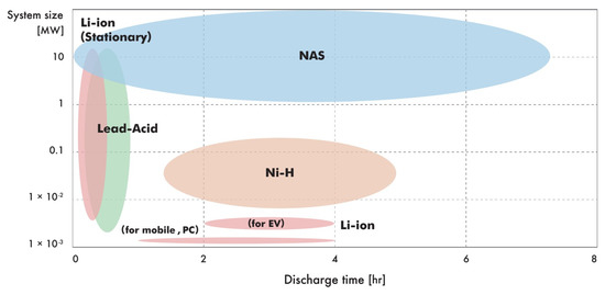
Figure 4.
System size Vs discharge comparison of common industrial batteries [44].
- Long duration
- High Power
- Long life expectancy
Furthermore, in Figure 4, the long duration feature illustrates that NAS batteries (among other kinds of batteries) are more suitable for large scale usagessuch as implementing them in wind power plantsand are able to produce energy three times more than lead acid batteries as a result of their “per unit volume”, which is also higher in comparison to lead acid batteries. NAS batteries are compatible with large scale plants such as wind or solar (10 to 100 s of MW). In order to control wind power plants at a large scale, NAS is the best choice in terms of its efficiency and compatibility [45,46]. One of the other features of this specific battery is its high capacity in terms of energy and its “long life span”, as it is counted at 100% depth of discharge (DOD) up to 2500 cycles [47,48]. To simplify the model, in this case of study, we assume all α, β and γ as constant for all x. Battery model parameters are defined in Table 1.

Table 1.
NAS battery model parameters.
Therefore, the nonlinear NAS battery model is as follows:
x (k + 1) = f (x(k)) + g(x(k), u(k))
Which based on the battery model parameters in Table 1, functions f and g are defined as:
f (x) = 0.98x
And;
In Equation (7), function f captures the state loss while energy is stored in the battery. Rate of loss is defined by battery self-discharge rate (0 < α(x) < 1) which varies on x.
The absorbed energy in the battery is represented by g in Equation (8) as a function of f needed energy (u(k)) and amount of energy inside the battery (x(k)). For positive input energy, the battery will be charged by the rate of β(x) (0 < β ≤ 1) until it gets saturated at Mc. The same trend is observed in the discharging process by rate of γ(x) (γ ≥1) when input energy is negative. Depending on the amount of state x, α, β, and э will be changed. In general, there is a contrariwise relationship between x and these coefficients. This idea stems from the fact that if the battery reaches its full capacity, a higher percentage of energy is lost inside it. By experimental examination on the battery, the re-link between x, β, and γ and x can be determined.
2.4. Reference Generator Model
The reference signal or target output should be defined for any closed-loop control system, in accordance with the desired system specifications and control objectives. We therefore propose to establish the reference signal via a decision-making method. The dynamics of our reference generator are as a battery state fraction and wind power expected. Mathematically, the decision-making mechanism is expressed [14]:
where yref(k) is the power signal reference, r(k) is the wind power forecast, and x2(k) is usable battery power. The Battery Plus Wind Power decision weight is w and is represented by,
This is the best nonlinear exponential parameter function. Two key principles underlie the proposed decision system:
- When the wind power is low, we supply the grid with electricity (with less storage and more supplies) wherever possible.
- Whenever the wind is high, we save as much energy as possible into the battery (it means more storage and less grid delivery).
We consider that a fraction of the energy available (battery + wind) is supplied to the grid for implementation of our decision-making method, and that is specified by (2w − 1). We call this “weight function” accordingly.
2.5. Wind Power Prediction Model
To increase the overall efficiency of the control system, a wind farm prediction system is combined with the energy saving system. Here we have a method of estimation for short-term wind power. The science of forecasting weather using atmosphere patterns and statistical techniques is the numerical weather prediction (NWP). At the input of the atmosphere mathematical models, existing weather conditions are used to forecast the weather [49].
The model proposed consists of two stages: (1) wind speed and direction prediction model and (2) the direction dependent power curve model. The prediction of wind vectors and, consequently, predictions of speed and direction are achieved using multiple observation points in the first stage. The second stage, using direction-dependent power curves, converts the predicted wind speed to the predicted output power. Figure 5 presents a schematic diagram of the weather device [49].
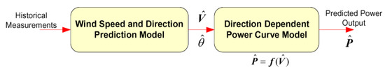
Figure 5.
NWP Model scheme schematic [50].
The advantages of the proposed solution are based on the use of many observation points leading to performance improvements. The NWP model data further improved marginally for a 10-min wind speed forecast. The final wind power forecast was thus substantially improved [49].
Data from NWP are collected from the wind farms in the Western Cape of South Africa and are expected to provide ideal wind speed data for ten minutes.
The data collected to study the generation volume and losses produced by the wind farm were considered in the parcels and thoroughly discussed in the Results and Discussions in Section 4.
2.6. Dynamic Controller Design
MPC is based on the solution of an optimal online control problem where a retrograde horizon approach is used in order to solve an optimum control problem for any current x(k) status at k for a potential open loop interval taking the constraints of present and future conditions into account [30]. The MPC algorithm measures an open loop sequence of manipulated variables such as the plant’s potential behavior. The first optimization value is then introduced into the factory. The status x(k+1) of this process is repeated at time (k+1). The MPC’s ability to comply with limitation and its use in practice and online optimization are some of the key advantages. Figure 2 shows the layout of the proposed control system. The proposed system control law in (1) will therefore be accomplished by minimizing the costs feature as follows [14]:
where N is the horizon of the forecast. The dynamic programming algorithm subject to the device model Equation (1) and following constraints is the optimization mechanism in this minimization analysis (11).
x2min ≤ x2(k) ≤ x2max
−Umax ≤ u(k) ≤ Umax
0 ≤ x1(k) ≤ c1
For all k ∈ 0,..., N − 1 with a given initial condition for (x1) and (x2) as (x1(N0)) and x1(N0) respectively.
There are some constraints which imposed by this system that indicated by (12), (13), and (14). The BESS cannot be discharged less than x2min or charged above x2Max, because the battery cannot exceed or be overloaded by the loading of a battery. Cell voltage of fully loaded cell (Umax) and Cell voltage of discharged cell (Umin) in Equation (13) reflects the maximum battery loading or unloading capacity. To keep the output of the system between 0 and rated value of the wind power (c1), constraint (10) is introduced.
We first implemented a function to enforce a dynamic programming procedure:
where M is the horizon of influence. This equation is determined by the full method searching 0 to x1(k) to c1; x2min to total x2(k) to total x2, to x1 to x2max; x2 to take x1 to 0 to every step; x2 to 0 to M + N to every step. For simplicity, the MPC algorithm uses wind energy estimation to be similar and equal to three (N = M = 3) in a control horizon.
We take it for granted first:
We suppose that,
We assume that we want to optimize J (x1, x2, M):
To calculate J*N0, we search all x1, x2 in full, taking into account the constraints that have been established to find y (N0) for all −Umax ≤ u ≤ Umax with small steps from our proposed models (4.1). After we have found an optimal value for J*N0, we will go to the next step to find J*N0+1 and find J*N0+M again. The optimal signal control sequence uopt(k), is found for k = {N0, …, N0 + M} at the end of the optimization cycle.
uop = {uop(N0), uop(N0 + 1), …, uop(N0 + M)}
The first value of the sequence (uop(N0)) is then selected as the first optimization value and implemented in the plant. This process is repeated (k +1) and the new step N0 is N0 + 1, and according to the model, the present state is x(k + 1). For our entire path, this procedure is repeated. DIgSILENT is power system analysis software application for use in analysing generation, transmission, distribution, and industrial systems. The software offers an extensive library of models of power system components and solves the problem of optimization at every stage [51].
3. Case Study
This study is of a Wind Farm situated in 35 km NE of Malmesbury, in the Western Cape of South Africa. The Wind Farm has a total of 46 wind turbines. Each turbine has a hub height 100 m, concrete towers, three blades, Double Fed Induction Generator (DFIG), Hydraulic Pitch control, and 12 kV with an out power of 3 MW totaling up to a capacity of 138 MW. It is connected to a 132 kV Distribution network at Windmeul Substation (Wellington), and is Germanischer Lloyd (GL) Certified and Grid Code Compliant. The initial construction started in March 2013 with a commercial operation date of July 2014. The owners are Acciona (54.9%), Royal bafokeng Holdings (25.1%), Soul City (10%), and Gouda Wind Energy Community Trust (10%) [52]. Below is the Cape Town wind farm and Acciona wind turbine (Figure 6).
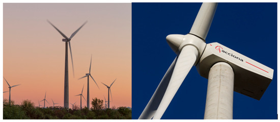
Figure 6.
Cape Town wind farm and Acciona wind turbine [53].
3.1. Data Collection
The real wind farm data is used to model the proposed system of control in DigSILENT software. The data obtained from the wind farm network in this simulation consists of 46 wind turbines, total capacity of 138 MW and connected to a 132 kV distribution network. Different wind measurements were carried for each month through the year 2016 to 2019. The wind data obtained includes hourly and monthly average wind speeds for each hour in the month. Calculations were performed on these data for each month to obtain the duration in hours for each 1 m/s speed range selected. The total wind speed range was divided into 1 m/s speed ranges taking the ranges: 0–1, 1–2, 2–3, 3–4, and so on. For each month, average wind speed, percentage of occurrence of each wind speed, power density for each wind speed and the total energy available in wind are calculated (Figure 7).
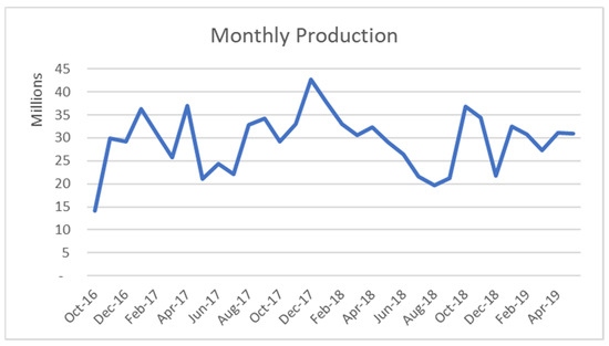
Figure 7.
Energy Generation Monthly Production [54].
The above energy generation assisted in battery size selection. For the wind data of the area and energy generated by each turbine average data from January to June over 2016 to 2019 for a wind turbine was collected.
Table 2.
2016 to 2019 January to June production average and capacity factor [54].
Table 3.
2019 January to June production average and capacity factor [54].
Moreover, a 2019 January to June production average and Capacity factor is shown and data is plotted in power diagram in respect to wind turbine power curve (Table 3).
Wind they do not produce continuous electricity. The capacity factor thus accounts for the estimation of the wind turbine output for a given period, divided by its output if the turbine has worked for the whole time (e.g., daily, weekly, yearly, etc.). The average capacity factor is 0.25–0.30 and the excellent capacity factor is approximately 0.40. The average speed directly affects the wind turbine capacity factor [55].
3.2. Battery Selection Type
The battery used was 50 MW NAS (sodium–sulfur), as the site’s current largest device is 50 MW, 300 MWh [48]. The data on the NAS battery (Figure 8) was therefore obtained from the company NGK insulators. This battery is 1.2 MW and 8.64 MWh in terms of power capacity. A total of 42 batteries are considered to make up 50,4 MW and 362.88 MWh in terms of power capacity for this study (Table 4). We used the following parameters for the battery model:
α = 0:98, β = 0:95, γ = 1:05, Md = 138 MW and Mc = −50.4 MW

Figure 8.
Sodium–Sulfur (NAS) Package type unit [48].
Table 4.
Simulated Constraints Parameters [48].
3.3. The Study
The study was conducted in DIgSILENT PowerFactory 2020 SP2A (x64) simulation software package. The scope, data collection, battery selection type, modelling, and result and discussion are outlined in subsections.
The simulation of both sections consists of the dynamic control of an integrated wind farm energy storage device linked to the grid. First, the battery voltage and current in the charging and discharging process is monitored. The second is a remedy or inverter, which can convert the DC voltage from the storage component into the AC voltage required for the grid [56].
Normally the rectifier or inverter is based on a pulse width modulation (PWM), voltage-sourced converter (VSC). This is well-known in PowerFactory and is available. The storage component of a rechargeable battery in this case is an element depending on the application. There is an issue with the broad variety of technologies inside a battery. So, for all batteries, there is no clear precise model [14,57].
Below we outline the network simulation and study cases.
3.4. Network Simulation
The wind farm network consists of 46 wind turbines, 12 kV with an output power of 3 MW and a total capacity of 138 MW. The 46, 12 kV wind turbines are parallel connected to the three, 50 MVA 132/12 kV step-up transformers. There is BESS of NAS with 42 kit enclosures and battery modules, consisting of 1 680 NAS modules, each rated at 30 kW and 216 kWh, with a rated performance of 50.4 MW and 201.6 MWh. The grid model consists of a 132 kV, 50 Hz, 40 KVA grid supply stage. With PowerFactory, it is easy to get a full report of all the active or reactive power installed, the installed energy, and the spinning reserve installed in the model. The cumulative load is assumed to be 300 MW. The minimum load case is 150 MW of the full load. Service Scenarios are used in PowerFactory for various load scenarios.
3.5. Study Cases
The study cases consist of three parts. The first part is a simulated battery load flow and fault analysis. The second component is load shift for which two experiments are used in the PowerFactory project: one with and one without BESS. The third element is a simulated 20% wind farm outage of wind turbines. Primary control energy is required in the grid to control the frequency within a very limited distance between the upper and lower frequency limits. In South Africa, the Grid Code for Renewable Power Plants is only 47–52 Hz with a minimum accuracy of 10 mHz in both positive and negative directions [57]. The grid already mentioned is used for the following investigation. The PWM converter has a rated capacity of 30 MVA. This corresponds to the frequency control bias already stated with a frequency bias of 30 MW/0.2 Hz = 150 MW/Hz. A sudden change in load in 30 MW of active power (simple connection of additional load) is simulated to test the BESS.
A frame and a DIgSILENT (DSL) model (like the battery model shown in Figure 9) are only the definition Frame for the Battery Model in DSL (.BlkDef), similar to a type of line or transformer. The entity of a frame is a composite model (ElmComp). The entity of a DSL model is a common model (ElmDsl) (see Figure 9).
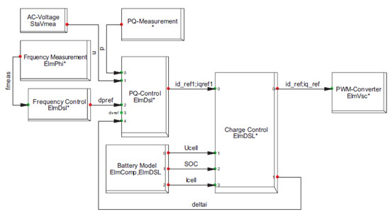
Figure 9.
Frame for the BESS-Controller [11].
The inputs, known from the load flow results in Figure 9, are ref/iq ref—(the currents in the dq-frame in p.u.) known from the PWM-converter, fmeas—(the frequency in p.u.) known from a PLL measurement, device (the absolute AC-voltage in p.u.) known from a voltage measurement device, and p - (the active power in p.u.) known from power measurement device. Active/reactive power measurement (PQ-Measurement), active/reactive power controller (PQ-Control), charging controller (Charge Control), and pulse width modulation (PWM) Converter. Ucell is the maximum or minimum voltage, State of Charge (SOC), and Icell is the charging or discharging current.
4. Results and Discussion
All the simulations were conducted in a computer with an Intel Core i7 CPU of 3.1 GHz, a RAM of 8 GB, and a 64-bit processor in the DIgSILENT PowerFactory 2020 SP2A (x64) simulation software package.
4.1. Study Case 1: Load Flow and Fault Analysis
4.1.1. Load Flow
Figure 10 below shows the State of Charge (SOC) graph. The initial SOC is set to 0; the SOC is determined to be 0 at 10.103 s of simulation time, slowly increasing with time, at 733.032 s of simulation time, the SOC is determined to be 0.44 at 1578 s of simulation time. The SOC is estimated to be 0.997, it can then be concluded that the BESS charge is approximately 15,580 s of simulation time. The external demand for energy is expected to be poor during the periods highlighted.
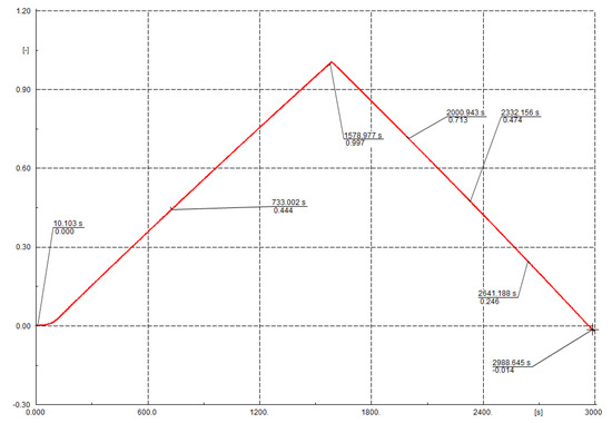
Figure 10.
State of Charge (SOC).
Once the BESS is fully charged, the SOC shall be equal to 1 and shall be ready for loading energy as per demand requirements. As can be seen from Figure 8, the charge status is progressively reduced to zero, which means that the power is sent to the load. At 2000 s, the SOC is estimated to be 0.713 out of 1 and decreases as time passes before the demand for the load or the battery is completely discharged. As estimated at 2988 s, the SOC is −0.014, which means that the BESS is totally discharged.
Figure 11 below shows the voltage charge of the battery rising in relation to the SOC as shown in Figure 6. At 1572 s, the voltage set-point is 1.023, which is while the battery was fully charged and S0C = 1. Voltage set point steadily decreases in proportion to the discharge time of the battery but does not exceed 0.p.u since the discharge depth is set to 80%.
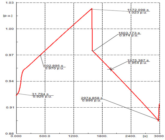
Figure 11.
Battery Voltage.
Figure 12 below indicates the active power of the battery. Before the simulation started, the active power of the battery was zero but steadily increased with the charging status. Negative active power depicts the energy expended by the battery as it is dispatched when the charging state reaches 1. Positive active power is an example of the power transmitted to the external load.
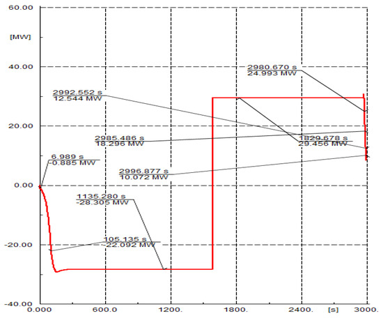
Figure 12.
Battery Total active Power in MW.
The battery therefore seemed to be operating and performing as planned under normal operating conditions. During peak demands, the BESS re-supplied the load once the charging status was reached, which means that the energy reserve was efficient based on the above-mentioned figures (Figure 10, Figure 11 and Figure 12).
4.1.2. Fault Analysis
The charging status of the battery is presumed to be 1, which means that the battery was fully charged prior to the simulation phase. The single-phase earth was generated at the coupling point for 5 s, the fault begins at 30 s of simulation time and is cleared at 35 s of simulation time. Below, Figure 13 indicates the voltage dips and the frequency deviation.
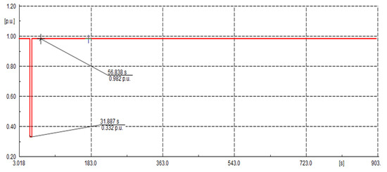
Figure 13.
Voltage magnitude at POC busbar (bus).
From the above Figure 13, it can be seen that the presence of BESS in the device network plays an important role in stabilizing the voltage magnitude in the collector bus to 0.332 p.u., compared to 0 p.u. without BESS. This means that the BESS was injecting reactive current into the grid to regulate the voltage while the device frequency was stabilizing to the minimum and maximum operating limits as shown in Figure 14 below.
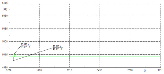
Figure 14.
Frequency at POC bus.
When the single phase fault occurred at external system busbar, it immediately created a voltage dip to 0 p.u. as shown in Figure 15, and the system voltage was restored after the fault was clear. Figure 15 shows a voltage dip that occurred at the system busbar to 0 p.u., once the fault was cleared after 5 s, the system voltage was restored back to 1 p.u.
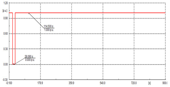
Figure 15.
Voltage Magnitude at Grid bus.
When the fault occurred at external grid, the frequency deviated above maximum and minimum operating limits but was cleared again after 5 s. This means that the system continues with normal operating conditions under acceptable limits of frequency and voltage. At POC (external Grid, frequency deviating between 65 Hz and 33 Hz) when the fault occurred, system frequency was restored back to 50 Hz after the fault was cleared, as shown in Figure 16.
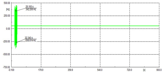
Figure 16.
Frequency at Grid bus.
4.1.3. Discussion
Fault analysis according to IEC60909/VDE0102 is not possible with a BESS because devices with power electronics like the pulse width modulation (PWM)-converter are not considered as the norm. But DSL also offers the possibility to calculate a short circuit according to the so-called complete method. The complete method also takes the load flow into account. Furthermore, it is possible to configure the PWM-converter model for the complete short circuit method. The two options are constant current or constant voltage. For an IGBT-based converter, a “constant I” current would be the right choice because the valves of the converter are only designed for a certain maximum current. To obtain the maximum current with the complete fault analysis the PWM-converter must be configured to full active power on the load flow dashboard. The fault results were achieved in this study by configuring the PWM-converter to full active power.
The BESS can only consume active power if the battery is not fully loaded (SOC < 1). The BESS can also only supply active power if the battery is not discharged (SOC > 0). The battery should thus be recharged if the SOC is below a certain level.
Therefore, the BESS can control the active power in both ways. The total output of active and reactive power should together not be bigger than the apparent rated power. Hence a priority for the active or reactive power is needed. All the conditions were fulfilled from a charge controller. For the results it was assumed that the SOC was available as a signal. The SOC can also be calculated from the battery current and voltage. All tasks and conditions for the controller were known and the design in DIgSILENT was activated. In [15,23], for a better overview it is recommended to divide the whole controller in smaller parts:
- Frequency controller (Frequency Control)
- Active/reactive power controller (PQ-Control)
- Charging controller (Charge Control)
The frequency controller is a simple proportional controller with a small dead band. In this case study, power system, it was important that there was only one integrator that controlled the frequency, otherwise we could have experienced problems with oscillation. The frequency control determined how much active power was activated in a case of a frequency deviation. Granted that K = 0.04, then the full active power of the BESS is activated if the frequency deviation is equal or greater than 2 Hz. The resulting values were in per unit values. The frequency control was coordinated to fulfil grid code requirements in a certain application case. In Figure 9, the command variable is f0, during the initialization process this value is fixed to frq (normally 1) with the command including(f0) = frq. The block ”offset” with the output ”p 0” is used to compensate ”dpref” if that value is not equal to zero after the load flow (because ”p_order frequ” is always zero after the initialization).
4.2. Study Case 2: Load Change
During the simulation without the BESS (study case: load without BESS) all governor controllers were tuned with standard values. Evidently, a load change of nearly 10% of the total grid load caused a big frequency under-run (red curves in Figure 13, Figure 14, Figure 15, Figure 16, Figure 17, Figure 18, Figure 19 and Figure 20). The compensation is important for the grid because it was able to increase the active power output much faster than the wind farm. A frequency of nearly 49 Hz would lead the grid to severe action. The BESS replaced the primary control power of the wind farm in the second simulation (study case: “load with BESS”). The turbine control of the wind turbine was modified for this purpose. The benefit for the controller was reduced from the normal value (K = 25) to K = 1. The participation of the wind farm in primary control reduced to almost zero. With the fast BESS, the underrun frequency was stopped and stabilized within a 200 mHz radius. The following section discusses 150 MW, Load Step down (−30 MW), and 30 MW Load Step up (+30 MW minimum) respectively.
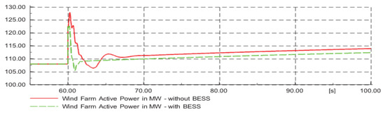
Figure 17.
Wind Farm Active Power with and without BESS.
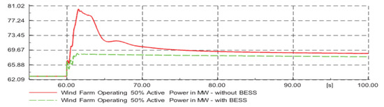
Figure 18.
Wind Farm 50% Active Power with and without BESS.
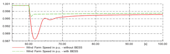
Figure 19.
Wind Farm Speed in p.u. with and without BESS.
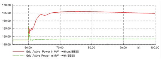
Figure 20.
Grid Active Power with and without BESS.
4.2.1. Load Step Down (−30 MW)
Wind Farm: Figure 17, shows the wind farm with and without battery storage facility. It can be noticed that variations from 60 to 70 s without a battery storage device are severe. With the implementation of BESS, fluctuations were mitigated, and the output power control system has been improved.
Figure 18 below, indicates a 50 percent wind farm with and without battery storage facility. Similarly, when the Wind Farm runs at maximum capacity, variations from 60 to 70 s without a battery storage system are serious. The difference, however, is that with the BESS implementation, fluctuations are minimized much more rapidly.
Figure 19 below shows the response of the wind farm to the period when the load was a phase. It can be deduced that without BESS it will take longer to stabilize because of the loss of control. Introduction of BESS reduces this time and enhances the weakness of the wind turbine control system to generate reliable power during load changes.
Grid: The grid response in Figure 20 when step load was provided created severe output power fluctuations while not supported by BESS. The implementation of BESS mitigates these variations and ensures the reliability output power supply for the load.
4.2.2. Load Step Down (+30 MW)
Wind Farm: For both Figure 21 and Figure 22, seven minutes after the loading step, the active power of the wind farm power plant increased by the order of dispatch. Power rose from 105 MW to 125 MW and 63 MW to 78 MW in five minutes, respectively. This is equal to a gradient of just 2.6 percent/min. The BESS wind farm was unburdened by quick load changes.
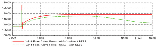
Figure 21.
Wind Farm Active Power with and without BESS.
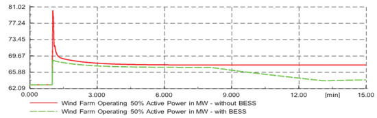
Figure 22.
Wind Farm 50%Active Power with and without BESS.
Figure 23 below shows the response of the wind farm to the time when the load was phased. Seven minutes after the loading phase, the order of dispatch increased the wind speed of the wind farm power plant. It can be deduced that it takes roughly the same time with and without BESS to stabilize since the load being supplied was larger than full capacity. Therefore, the introduction of BESS reduces this time by marginally improving the wind turbine control system to produce reliable power during load changes.
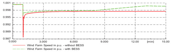
Figure 23.
Wind Farm Speed in p.u. with and without BESS.
Grid: It can be deduced from Figure 24 below, that during full load Grid variation was large and the introduction of the BESS power was stable from 150 MW, then after some time rose to 170 MW. The implementation of BESS stabilizes the grid and mitigates these variations and ensures the reliability output power supply for the load.
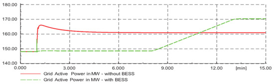
Figure 24.
Grid Active Power with and without BESS.
4.2.3. Discussion
For a steady state load flow analysis, the are no further dynamic models needed of the wind farm BESS. Only the generator types of power plants and the information on the load flow page were configured. This information also includes the capability limit curve for reactive power. It is important to have one reference machine in the grid. The generator from the wind farm is the reference in the sample grid. The BESS controls the active power output and the local voltage. If the load flow is calculated with the option ”Active Power Control according Secondary Control” then it is possible to configure the participation of the plant on the compensation of a load change with the variable ”Primary Frequency Bias” (Kpf). The turbine governor controls the speed of the turbine and so, via the synchronous machine, the electric frequency. In [6,7], in the case of a fast load change, the frequency rapidly dropped due to the lack of active power in the grid. To prevent a slowdown of the whole system the turbine governor must activate more power. This is called primary frequency control (or also spinning reserve), and activation must be instantaneous. This means that a grid is constantly losing energy due to permanent choking on the turbine valve. Therefore, it would be more economical if another device could deliver the primary control energy until the wind farm has increased the active power. This is called secondary frequency control; activation must occur within 15 min after the frequency deviation. To fill that gap a BESS was used as a solution on this study. The simulation results on load changes confirm the BESS fills the gap.
4.3. Study Case 3: Wind Farm Outage
The case of a wind farm 20% outage (111 MW = 9 wind turbines are switched off 27 MW) in a small showcase grid is an outage of the wind turbine. Without this fast-controlling plant, it would be much harder to regulate the frequency after a disturbance. To research the outage with more practical performance, only 80 percent of the original loads are believed to have a low load scenario (Loads = 150 × 0.8 = 120 MW). This is the operating scenario used in PowerFactory.
For an operating situation, it is possible to adjust and store operating data in various situations, such as a low load and a high load event, without the need for additional variance. The shutdown of the wind farm with the wind turbine and grid is simply simulated by opening the switch on the HV side of the main transformer. The following frequency under-run is more distinct from the load shift chase without the BESS. This is due to the lack of a fast-controllable power plant.
Again, the BESS is used to improve the behavior of the grid performance and to replace the primary control power of the grid. Below are the results obtained from DIgSILENT and clearly explained.
4.3.1. Wind Farm 20% Outage Load Step Down (−30 MW)
Wind Farm: From Figure 25, we see that the wind farm took approximately 18 s to monitor the fluctuation of the power output. With the implementation of BESS, the active power output was regulated within 7 s—much faster than the power plant because there was no mechanical inertia and delay. The frequency deviation was also lower.
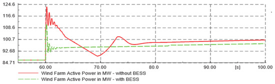
Figure 25.
Wind farm Wind Farm Active Power with and without BESS.
Figure 26 below shows the response of the wind farm to the time when the outage and load was phased. For “with” and “without BESS”, it took approximately 15 s to control the wind turbine speed minutes after the loading phase, however in terms of speed there is a difference of 0.029 p.u. Therefore, the introduction of BESS improved wind turbine output power control during the outage and load change.
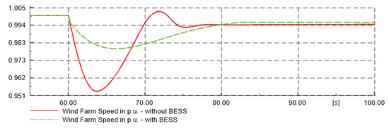
Figure 26.
Wind Farm Speed in p.u. with and without BESS.
Grid: The grid response in Figure 27, outage and load when phased is provided. The response of grid creates severe output power fluctuations while not supported by BESS. The implementation of BESS mitigates these variations and ensures the reliability output power supply for the load.
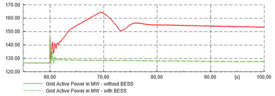
Figure 27.
Active Power Active Power with and without BESS.
4.3.2. Wind Farm 20% Outage Load Step Down (+30 MW)
Wind Farm: The wind farm can be deduced from the fact that the load increased in Figure 28. With BESS, the active power output was controlled within a minute—much faster than the power plant since there was no mechanical inertia and delay. The frequency deviation was smaller, too. It should be noted that the power supplied by the wind farm and the batteries steadily decreases since the power of the battery decays with time.

Figure 28.
Wind farm Active Power with and without BESS.
Figure 29 below shows the reaction of the wind farm to the time the outage and load was phased out. It took about a minute to monitor the wind turbine speed, both with and without BESS, minutes after the loading process, but in terms of speed the wind farm speed fluctuated between 16 and 21 min. With the implementation of BESS, the speed remained constant, which increased the power output control of the wind turbine during outage and load change.
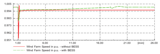
Figure 29.
Wind Farm Speed in p.u.
Grid: The grid response in Figure 30, and outage and load when phased is provided. The response of the grid without BESS took approximately 3 min to control fluctuations, remain constant, and not meet the load demand. The implementation of BESS mitigated with a minute these variations and increased output power to ensure it met the load demand.
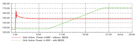
Figure 30.
Active Power Active Power with and without BESS.
4.3.3. Discussion
The study simulated different outages in the time domain, a 20% outage during step up and down, respectively. During an outage, primary control energy is needed in a grid to control the frequency within a very small gap between an upper and a lower frequency limit. The compensation must be activated within 30 s and the power must be continued for at least 15 min. In [24], demand from the grid is that each grid operator must deliver 2% of their actual produced active power as primary control power, the primary control power could also come from a BESS and the outage of a generator is a very big load change in the network. Therefore, due to the configuration of Kpf, it is possible to define a maximum frequency deviation. An outage of the wind farm (60 MW) should be compensated from the BESS within a frequency deviation of 1.5 Hz, then the Kpf-factor must be 20 MW/Hz (=60 MW/2/1.5 Hz). The transformers have automatic tap changers to control voltage on the high voltage side. To make sure that the tap changers work automatically and that the generators are inside their reactive power limits the options are: Automatic Tap Adjust of Transformers, and Consider Reactive.
5. Conclusions
In this study, we suggested a generic energy model for BESS that can be used in renewable energy plant applications based on all battery features and an extensive literature review of available battery models. We have given model parameters for the battery NAS as a case study. A nonlinear battery model was proposed in this study for integration with a wind farm to smooth output while the battery works on a safe margin. For dynamic control of wind farm BESS, the study developed a system based on MPC which could mitigate wind turbine variability and intermittence problems. The MPC controller operated well under very strict realistic restrictions from collected data, which guaranteed the system’s stability. The stochastic optimization of the proposed dynamic control approach of uncertain parameters as discrete or continuous functions of probability density was also investigated. The simulation results showed good performance of MPC in wind BESS tracking, including capacity, limited SOC, and power load/unload limits. It is not only wind power that the control scheme proposed. It can be used for other intermittent sources of energy, such as large-scale solar photovoltaic farms. In general, further research on the robustness, uncertainty, and noise effects in future works is essential to enhance the overall performance of the dynamic control wind farm BESS. The quality of our modelling through robust optimizations is another direction of future research.
Author Contributions
Conceptualization, methodology, software, validation, formal analysis, investigation, resources, data curation, M.G.; Conceptualization, methodology, writing—original draft preparation, writing—review and editing, visualization, supervision, project administration, A.R. All authors have read and agreed to the published version of the manuscript.
Funding
This research received no external funding.
Institutional Review Board Statement
Not applicable.
Informed Consent Statement
Not applicable.
Data Availability Statement
Restrictions apply to the availability of these data. Data was obtained from third party and are available from the authors with the permission of third party.
Conflicts of Interest
The authors declare no conflict of interest.
Abbreviations
| PV | Photovoltaics |
| IPP | Independent Power Producers |
| RESs | Renewable Energy Sources |
| DFIG | Double Fed Induction Generator |
| BESSs | Battery Energy Storage Systems |
| HAWT | Horizontal Axis Wind Turbine |
| VAWT | Vertical Axis Wind Turbine |
| kW | kilo Watt |
| WECS | Wind Energy Conversion System |
| EESS | Electrical Energy Storage Systems |
| AW | Action Windpower |
| WES | Wind Energy System |
| WTs | Wind Turbines |
| DigSILENT | Digital Simulator for Electrical Network |
| DoE | Department of Energy |
References
- Eskom. Application for a Generator Connection to the Eskom Network. 2013. Available online: http://www.eskom.co.za/Whatweredoing/Documents/IPP_GridApplicationForm_Rev8_5Nov2013.pdf (accessed on 19 April 2018).
- International Energy Agency. World Energy Outlook 2016 Part B: Special Focus on Renewable Energy. Available online: https://www.iea.org/media/publications/weo/WEO2016SpecialFocusonRenewableEnergy.pdf (accessed on 19 April 2018).
- Department of Energy. Integrated Resource Plan for 2010–2030. 2011. Available online: http://www.energy.gov.za/IRP/irpfiles/IRP2010_2030_Final_Report_20110325.pdf (accessed on 19 April 2018).
- Eskom. Grid Connection Code for Renewable Power Plants (RPPs) Connected to the Electricity System or the Distribution System in South Africa. 2014. Available online: https://www.sseg.org.za/wp-content/uploads/2019/03/South-African-Grid-Code-Requirements-for-Renewable-Power-Plants-Version-2-8.pdf (accessed on 18 February 2021).
- Kelly, J.J.; Leahy, P.G. Sizing Battery Energy Storage Systems: Using Multi-Objective Optimization to Overcome the Investment Scale Problem of Annual Worth. IEEE Trans. Sustain. Energy 2019, 11, 2305–2314. [Google Scholar] [CrossRef]
- Sheng, D.; Dai, H.; Chen, M.; Chi, Y. Discussion of wind farm integration in China. In Proceedings of the 2005 IEEE/PES Transmission & Distribution Conference & Exposition: Asia and Pacific, Dalian, China, 18 August 2005. [Google Scholar]
- Abhinav, R.; Pindoriya, N.M. Grid integration of wind turbine and battery energy storage system: Review and key challenges. In Proceedings of the 2016 IEEE 6th International Conference on Power Systems (ICPS), New Delhi, India, 4–6 March 2016; pp. 1–6. [Google Scholar]
- Ohki, Y. World’s Largest-Class Battery Energy Storage System. IEEE Electr. Insul. Mag. 2016, 32, 64–66. [Google Scholar] [CrossRef]
- Saber, H.; Heidarabadi, H.; Moeini-Aghtaie, M.; Farzin, H.; Karimi, M.R. Expansion Planning Studies of Independent-Locally Operated Battery Energy Storage Systems (BESSs): A CVaR-Based Study. IEEE Trans. Sustain. Energy 2019, 11, 2109–2118. [Google Scholar] [CrossRef]
- World Energy Council. Five Steps to Energy Storage. Innovation Insights Brief. 2020, p. 62. Available online: www.worldenergy.org (accessed on 18 February 2021).
- DIgSILENT GmbH. DIgSILENT PowerFactory Application Example Battery Energy Storing Systems. 2010, pp. 1–28. Available online: https://www.digsilent.de/en/faq-reader-powerfactory/do-you-have-an-application-example-for-a-battery-energy-storage-system-bess.html (accessed on 18 February 2021).
- Zakeri, B.; Syri, S. Electrical energy storage systems: A comparative life cycle cost analysis. Renew. Sustain. Energy Rev. 2015, 42, 569–596. [Google Scholar] [CrossRef]
- Fathima, A.H.; Palanisamy, K. Battery energy storage applications in wind integrated systems—A review. In Proceedings of the 2014 International Conference on Smart Electric Grid (ISEG), Guntur, India, 19–30 September 2014; pp. 1–8. [Google Scholar]
- Zarei Fard, M.T. Modelling and Control of Wind Farms Integrated with Battery Energy Storage Systems. Ph.D. Thesis, The University of New South Wales, Sydney, Australia, August 2017. [Google Scholar]
- Hansen, A.D.; Rensen, P.S.; Blaabjerg, F.; Becho, J. Dynamic Modelling of Wind Farm Grid Interaction. Wind. Eng. 2002, 26, 191–210. [Google Scholar] [CrossRef]
- Shi, R.; Li, S.; Zhang, P.; Lee, K.Y. Integration of renewable energy sources and electric vehicles in V2G network with adjustable robust optimization. Renew. Energy 2020, 153, 1067–1080. [Google Scholar] [CrossRef]
- Hosseini, S.M.; Carli, R.; Dotoli, M. A Residential Demand-Side Management Strategy under Nonlinear Pricing Based on Robust Model Predictive Control. In Proceedings of the 2019 IEEE International Conference on Systems, Man and Cybernetics (SMC), Bari, Italy, 6–9 October 2019; pp. 3243–3248. [Google Scholar]
- Banzo, M.; Ramos, A. Stochastic Optimization Model for Electric Power System Planning of Offshore Wind Farms. IEEE Trans. Power Syst. 2010, 26, 1338–1348. [Google Scholar] [CrossRef]
- Sperstad, I.B.; Korpås, M. Energy Storage Scheduling in Distribution Systems Considering Wind and Photovoltaic Generation Uncertainties. Energies 2019, 12, 1231. [Google Scholar] [CrossRef]
- Safdarian, A.; Fotuhi-Firuzabad, M.; Lehtonen, M. A Stochastic Framework for Short-Term Operation of a Distribution Company. IEEE Trans. Power Syst. 2013, 28, 4712–4721. [Google Scholar] [CrossRef]
- Mavromatidis, G.; Orehounig, K.; Carmeliet, J. Design of distributed energy systems under uncertainty: A two-stage stochastic programming approach. Appl. Energy 2018, 222, 932–950. [Google Scholar] [CrossRef]
- Ghasemi, A.; Banejad, M.; Rahimiyan, M. Integrated energy scheduling under uncertainty in a micro energy grid. IET Gener. Transm. Distrib. 2018, 12, 2887–2896. [Google Scholar] [CrossRef]
- Luta, D.N. Modelling of Hybrid Solar Wind Intergrated Generation Systems in an Electrical Distribution Network. Master’s Thesis, The Cape Peninsula University of Technology, Cape Town, South Africa, September 2014. [Google Scholar]
- Liu, Y.; Liu, S.L.; Wen, J.Y. Investigation on Control Strategies to Smooth out Wind Farm Output Fluctuations Using Energy Storage System. Appl. Mech. Mater. 2014, 521, 117–123. [Google Scholar] [CrossRef]
- Wang, W.; Ma, R.; Xu, H.; Wang, H.; Cao, K.; Chen, L.; Ren, Z. Method of energy storage system sizing for wind power generation Integration. In Proceedings of the 2016 IEEE PES Asia-Pacific Power and Energy Engineering Conference (APPEEC), Xian, China, 25–28 October 2016; pp. 1200–1203. [Google Scholar]
- Branco, H.; Castro, R.; Lopes, A.S. Battery energy storage systems as a way to integrate renewable energy in small isolated power systems. Energy Sustain. Dev. 2018, 43, 90–99. [Google Scholar] [CrossRef]
- Schaffarczyk, A. Understanding Wind Power Technology; John Wiley & Sons, Inc.: Hoboken, NJ, USA, 2014. [Google Scholar]
- Kulakowski, B.T.; Gardner, J.F.; Shearer, J.L. Dynamic Modelling and Control of Engineering Systems; Cambridge University Press: Cambridge, UK, 2013; Volume 53. [Google Scholar]
- Sperstad, I.B.; Helseth, A.; Korpas, M. Valuation of stored energy in dynamic optimal power flow of distribution systems with energy storage. In Proceedings of the 2016 International Conference on Probabilistic Methods Applied to Power Systems (PMAPS), Beijing, China, 16–20 October 2016; pp. 1–8. [Google Scholar]
- Yang, D.; Wen, J.; Chan, K.W.; Cai, G. Dispatching of Wind/Battery Energy Storage Hybrid Systems Using Inner Point Method-Based Model Predictive Control. Energies 2016, 9, 629. [Google Scholar] [CrossRef]
- Liu, W.; Liu, Y. Hierarchical model predictive control of wind farm with energy storage system for frequency regulation during black-start. Int. J. Electr. Power Energy Syst. 2020, 119, 105893. [Google Scholar] [CrossRef]
- Hu, J.; Shan, Y.; Guerrero, J.M.; Ioinovici, A.; Chan, K.W.; Rodriguez, J. Model predictive control of microgrids—An overview. Renew. Sustain. Energy Rev. 2021, 136, 110422. [Google Scholar] [CrossRef]
- Zhang, F.; Fu, A.; Ding, L.; Wu, Q. MPC based control strategy for battery energy storage station in a grid with high photovoltaic power penetration. Int. J. Electr. Power Energy Syst. 2020, 115, 105448. [Google Scholar] [CrossRef]
- Jadidi, S.; Badihi, H.; Zhang, Y. Passive Fault-Tolerant Control Strategies for Power Converter in a Hybrid Microgrid. Energies 2020, 13, 5625. [Google Scholar] [CrossRef]
- Rodríguez del Nozal, Á.; Gutiérrez Reina, D.; Alvarado-Barrios, L.; Tapia, A.; Escaño, J.M. A MPC Strategy for the Optimal Management of Microgrids Based on Evolutionary Optimization. Electronics 2019, 8, 1371. [Google Scholar] [CrossRef]
- Sun, Y.; Zhao, Z.; Yang, M.; Jia, D.; Pei, W.; Xu, B. Research overview of energy storage in renewable energy power fluctuation mitigation. CSEE J. Power Energy Syst. 2019, 6, 160–173. [Google Scholar] [CrossRef]
- Hosseini, S.M.; Carli, R.; Dotoli, M. Robust Optimal Energy Management of a Residential Microgrid under Uncertainties on Demand and Renewable Power Generation. IEEE Trans. Autom. Sci. Eng. 2020, 1–20. [Google Scholar] [CrossRef]
- Shepherd, W.; Zhang, L. Electricity Generation Using Wind Power; World Scientific: Singapore, 2011. [Google Scholar]
- Gustavo, M.; Gimenez, J. Technical and Regulatory Exigencies for Grid Connection of Wind Generation. In Wind Farm—Technical Regulations, Potential Estimation and Siting Assessment; IntechOpen: London, UK, 2011. [Google Scholar]
- European Wind Energy Association, “Contact,” 2021. Available online: https://www.wind-energy-the-facts.org/contact.html (accessed on 14 February 2021).
- Yun, P.; Ren, Y.; Xue, Y. Energy-Storage Optimization Strategy for Reducing Wind Power Fluctuation via Markov Prediction and PSO Method. Energies 2018, 11, 3393. [Google Scholar] [CrossRef]
- Palm, W.J. Basic Control Systems Design. Eshbach’s Handbook of Engineering Fundamentals; Wiley Online Library: Hoboken, NJ, USA, 2009; pp. 760–801. [Google Scholar] [CrossRef]
- Veldhuis, S.; Dosbaeva, G.; Yamamoto, K. Tribological compatibility and improvement of machining productivity and surface integrity. Tribol. Int. 2009, 42, 1004–1010. [Google Scholar] [CrossRef]
- NGK Insulators LTD. Case Studies 3,700MWh/530MW Effectively Stored and Utilized in 200 Locations; NGK Insulators LTD: Cape Town, South Africa, 2016. [Google Scholar]
- Tamyürek, B.; Nichols, D.K. Performance Analysis of Sodium Sulfur Battery in Energy Storage and Power Qaulity Applications. Eskişehir Osman. Univ. 2004, 17, 99–115. [Google Scholar]
- Hussien, Z.F.; Cheung, L.W.; Siam, M.F.M.; Ismail, A.B. Modeling of Sodium Sulfur Battery for Power System Applications. 2007. Available online: http://fke.utm.my/elektrika (accessed on 31 January 2021).
- Kamibayashi, M.; Furuta, K. High Charge and Discharge Cycle Durability of the Sodium Sulfur (NAS) Battery. Available online: https://www.sandia.gov/ess-ssl/EESAT/2002_papers/00021.pdf (accessed on 18 February 2021).
- NGK Insulators. About NAS Batteries, Products, NGK Insulators, LTD. 2020. Available online: https://www.ngk-insulators.com/en/product/nas/about/index.html (accessed on 1 September 2020).
- Khalid, M.; Savkin, A.V. Closure to discussion on “A method for short-term wind power prediction with multiple observation points”. IEEE Trans. Power Syst. 2013, 28, 1898–1899. [Google Scholar] [CrossRef]
- Khalid, M.; Savkin, A.V. A Method for Short-Term Wind Power Prediction with Multiple Observation Points. IEEE Trans. Power Syst. 2012, 27, 579–586. [Google Scholar] [CrossRef]
- Sørensen, P. Simulation of Interaction between Wind Farm and Power System; Risø DTU National Laboratory for Sustainable Energy: Roskilde, Denmark, December 2001. [Google Scholar]
- Kroes, J. Gouda Wind Facility NERSA Public Hearings Cape Town; NERSA: Pretoria, South Africa, 2012. [Google Scholar]
- Acciona Windpower. Unpublished Service and User Manaul AW 300; Acciona Windpower: Hamburg, Germany, 2011. [Google Scholar]
- Acciona Windpower. Unpublished Consolidated Generation Data; Acciona Windpower: Hamburg, Germany, 2019. [Google Scholar]
- Tong, W. Fundamentals of Wind Energy; WIT Press: Southamption, UK, 2010; Volume 30. [Google Scholar]
- Ma, Y.; Wu, L. A stimulation study of the dynamic power control method for VSCF doubly-fed induction wind turbine based on Labview. In Proceedings of the 2009 World Non-Grid-Connected Wind Power and Energy Conference, Nanjing, China, 24–26 September 2009; pp. 1–4. [Google Scholar]
- Paul, S.; Nath, A.P.; Rather, Z.H. A Multi-Objective Planning Framework for Coordinated Generation from Offshore Wind Farm and Battery Energy Storage System. IEEE Trans. Sustain. Energy 2019, 11, 2087–2097. [Google Scholar] [CrossRef]


Publisher’s Note: MDPI stays neutral with regard to jurisdictional claims in published maps and institutional affiliations. |
© 2021 by the authors. Licensee MDPI, Basel, Switzerland. This article is an open access article distributed under the terms and conditions of the Creative Commons Attribution (CC BY) license (http://creativecommons.org/licenses/by/4.0/).