Article

Factors Affecting COVID-19 Outbreaks across the Globe: Role of Extreme Climate Change

1
School of Atmospheric Sciences, Sun Yat-sen University, Zhuhai 519082, China
2
Guangdong Province Key Laboratory for Climate Change and Natural Disaster Studies, Sun Yat-sen University, Zhuhai 519082, China
3
Center for Monsoon System Research, Institute of Atmospheric Physics, Chinese Academy of Sciences, Beijing 100029, China
4
Institute of Atmospheric Physics, University of Chinese Academy of Sciences, Beijing 100049, China
*
Authors to whom correspondence should be addressed.
Sustainability 2021, 13(6), 3029; https://doi.org/10.3390/su13063029
Submission received: 27 January 2021 / Revised: 1 March 2021 / Accepted: 3 March 2021 / Published: 10 March 2021

Abstract

:
The Coronavirus Disease 2019 (COVID-19) pandemic poses a serious threat to global health system and economy. It was first reported in Wuhan, China, and later appeared in Central Asia, Europe, North America, and South America. The spatial COVID-19 distribution pattern highly resembles the global population distribution and international travel routes. We select 48 cities in 16 countries across 4 continents having infection counts higher than 10,000 (by 25 April 2020) as the COVID-19 epicenters. At the initial stage, daily COVID-19 counts co-varies strongly with local temperature and humidity, which are clustered within 0–10 °C and 70–95%, respectively. Later, it spreads in colder (−15 °C) and warmer (25 °C) countries, due to faster adaptability in diverse environmental conditions. We introduce a combined temperature-humidity profile, which is essential for prediction of COVID-19 cases based on environmental conditions. The COVID-19 epicenters are collocated on global CO2 emission hotspots and its distribution maximizes at 7.49 °C, which is 1.35 °C/2.44 °C higher than current (2020)/historical (1961–1990) mean. Approximately 75% of the COVID-19 cases are clustered at severe-extreme end of historical temperature distribution spectrum, which establish its tighter and possible association with extreme climate change. A strong mitigation measure is essential to abate the GHG emissions, which may reduce the probability of such pandemics in the future.

1. Introduction

The Coronavirus Disease 2019 (COVID-19) pandemic poses a serious threat to the human civilization and has triggered shockwaves to the global economy and healthcare system [1]. The COVID-19 was first reported in Wuhan, China, during December 2019 [2,3,4,5] and later spread to the other provinces and different countries across the globe [6]. According to a World Health Organization (WHO) report, the global risk assessment level for COVID-19 is still very high. The confirmed number of COVID-19 cases crosses 90 million worldwide and death toll exceeds 2 million in 219 countries [6].
It was found that for the Severe Acute Respiratory Syndrome-Coronavirus-2 (SARS-CoV-2) transmission, respiratory droplets and international travel routes are the dominant transmission modes causing the COVID-19 [7,8,9,10,11,12]. Usually, coronaviruses, like SARS-Cov-2 virus (100 nm diameters), require liquid nuclei to travel in the atmosphere or bond with the particulate matters (PM) e.g., PM2.5 and PM10, which acts as carrier for SARS-Cov-2 in the air [13,14]. It was reported that the aerosols with carrier particle size ≤ 5 µm diameter are appropriate for the airborne transmission of SARS-Cov-2 (Modes of transmission of virus, WHO Report). Weber and Stilianakis (2008) [15] and Pyankova et al. (2018) [16] reported that the existence and transmission of SARS-CoV virus and Middle East Respiratory Syndrome-Coronavirus (MERS-CoV-2012) in the atmosphere depends strongly on environmental factors e.g., temperature, humidity, solar intensity, etc. It was observed that the MERS-CoV virus is effective and survives at temperature around 25 °C and relative humidity higher than 79%. It remains infectious for 60 min after aerosolization [16]. Moreover, dry viruses can remain active on smooth surfaces for ~5 days and at temperatures and relative humidity within 22–25 °C and 40–50%, respectively [17]. There are several studies showing that meteorological factors alone may not explain most of the variability of the COVID-19 outbreak (Mecenas et al., 2020 and references therein) [18], however, they might facilitate the virus transmission. Public isolation policies, herd immunity, migration patterns, containment measures, population density, and cultural aspects directly influence how the spread of this disease occurs. According to Oliveiros et al. (2020) [19], temperature and humidity contribute to a maximum of 18% of the variation, the remaining 82% being related to other factors. Sasikumar et al. (2020) [20] selected 20 densely populated cities of India as COVID-19 hotspots and reported a strong covariability with local temperature at the initial phase of the outbreak. They showed that local temperature accounts approximately 65–85% of the explained variance, i.e., the spread of COVID-19 depends strongly on local temperature rise prior to the community transmission phase.
The impact of climate change on epidemiology of zoonotic disease [21] and their transmission from animal species to human [22,23] are well reported. Global warming induced extreme weather events have a strong negative impact on the biodiversity and seasonality of different vector borne diseases [24]. For example, the West Nile fever and Lyme disease are the cause of climate change induced zoonosis [21]. In general, bats are the natural reservoir or the potential source for the SARS-CoV [25]. In recent decades, the Earth has experienced an increase in greenhouse gas emissions due to unprecedented burning of fossil fuel, which causes the global mean temperature to increase at a rate of 0.2 °C/decade and predicted to reach 4 °C by the end of 21st century [26]. Subsequently, it increases the frequency and intensity of heat waves and heat stress, which may disrupt the metabolism, increase the oxidative stress, and suppress the immune system, causing infections and release of the viruses to the environment [27] (more in Supplementary Information 1).
In the current manuscript, we investigate the role of population density, international air travel, pollution, temperature and humidity underlying the rapid spread and transmission of the SARS-CoV-2 virus, globally at its initial phase. Here, we define the severity of COVID-19 from its cumulative counts over the epicenters. Figure 1 represents the distribution of COVID-19 cases globally. The regions with higher cumulative counts are extremely severe, while with less cumulative counts are less severe. Furthermore, we establish a tighter relationship between emissions induced extreme climate change and the COVID-19 pandemic. In addition, we ascertain that the differences in health systems and governmental strategies may influence spread and magnitude of the pandemic. However, the actions taken so far are “slow and insufficient” with “scrambling to implement appropriate measures to delay spread of the virus” [28]. We also analyze the spatial pattern of the COVID-19 infected territories and gradual emergence of the epicenters across the globe. The research results are novel and of utmost importance to understand and contain the spread of the SARS-Cov-2 virus in the future.

2. Population Density

Respiratory droplets and contact routes are the fastest modes of COVID-19 transmission across the globe [12]. In addition, population density plays a significant role in its transmission. At the beginning of the outbreak, the epicenters or the COVID-19 hotspots are clustered in the northern hemisphere (Figure 1, Table 1), centered in Wuhan (China), Singapore and Iran in Asia, Turkey, United Kingdom (UK), Italy, Spain, Portugal, France, Belgium, Netherlands, Germany in Europe, Canada, and the United States of America (USA) in North America, Russia, and Sao Paulo (Brazil) in South America. The hotspots or the epicenters are selected based on the number of COVID-19 cases exceeds 10,000 (extremely affected) by 25 April 2020. Based on the above criteria, we have selected 48 cities in 16 countries across 4 continents (methods).
Due to more landmass, approximately 88% of the global population resides in northern hemisphere, particularly beyond 23° N. The population density (Supplementary Figure S1a) is highest in East and South Asian countries (China, India, Japan, Korea, and Thailand etc., 250–1000+ i.e., severe to extremely dense), Central Asia (25–250 i.e., highly dense), Europe (25–250+ i.e., high to severely dense), western part of Russia (5–250 i.e., moderate to highly dense), eastern coast of USA (5–250 i.e., moderate to highly dense), central-southern Africa (25–250+ i.e., high to severely), and coastal Southern America (5–25 i.e., moderately dense) (SEDAC, 2020) [29]. As a consequence, the COVID-19 epicenters are collocated on the regions of higher population density and its global distribution pattern resembles clearly with the population density distribution across the globe, except in the African continent (more in Supplementary Information 2). Therefore, the higher the population density, the higher the proximity between people, and the higher the risk of COVID-19 infection is.

3. International Air Transport Traffic

It is well known that the wide scale human migration and international travel can transform a localized outbreak into a widespread pandemic [30]. The COVID-19 pandemic poses an extreme threat to the travelling public because intercontinental travel is one of the fastest modes of transmission of the novel pathogens [31]. Therefore, airports and international air transport routes are vulnerable to COVID-19 virus transmissions. Supplementary Figure S1b shows the worldwide distribution of airports [32] and air transport traffic statistics [33]. The big clusters of airports are centered over Europe stretching southeastward to Central Asia, South Asia, East Asia, and Southeast Asia. In North America, the airports are clustered mainly in the eastern part of USA, California in the west coast, eastern Canada (Quebec, Ontario), Mexico, and the Caribbean islands. In South America, the airports are clustered in Venezuela, Colombia, Ecuador, and Peru in the west coast and Brazil in the east coast. Moreover, the international air traffic accounts approximately 55.7% in Europe, 44% in Asia, and 28.9% in North America, whereas it is only 7.4% in South America, 5.8% in Africa, and 5% in Australia. Like population density, the worldwide distribution of airports correlates strongly with the COVID-19 pandemic distribution pattern. Despite higher population density, the African continent has experienced a lesser number of SARS-CoV-2 cases, which is possibly due to the lesser number of airports and limited international air traffic movements. Therefore, the higher the density of airports and international travels, the higher the risk of SARS-CoV-2 virus transmission. However, it is worthy to mention that many of the underdeveloped countries have deficiency in the health care system and may have not done enough testing to detect the actual spread of this virus (Bukhari et al., 2020) [34].

4. Pollution

The epidemiology of infectious diseases has a close association with the atmospheric pollutants like ozone, SO2, NO2, and Particulate Matter (PM). Due to higher ozone and PM levels, respiratory infections affect the immune system and have a strong association with influenza and pneumonia, respectively [35,36]. It is not only the impact of pollution on the human immune system; usually the viruses interact with the pollutants, and remain airborne for longer time, which make their way to the lungs. Moreover, in air, coronaviruses may infect after 60 min of aerosolization [16] (more in Supplementary Information 3).
A statistical relationship between the concentrations of PM, CO, NO2, ozone, and COVID-19 was demonstrated in 120 cities in China [37]. Fattorini et al. [38] demonstrated using the air-quality data of 71 Italian provinces that air pollution correlates with COVID-19 cases [38]. Pansini et al. [39] investigated this worldwide and demonstrated that infection spreading was correlated with several annual satellite and ground indexes of air quality in China, the USA, Italy, Iran, France, Spain, Germany, and the UK. They found a higher incidence of SARS-CoV-2 in areas with high PM and NO2 concentrations. The study by Pozer et al. [40] demonstrated that particulate air pollution contributed 15% to COVID-19 mortality worldwide, 27% in East Asia, 19% in Europe, and 17% in North America and that globally, 50–60% of the attributable, anthropogenic fraction is related to fossil fuel use, up to 70–80% in Europe, West Asia, and North America.
In the decadal mean (1998–2012) PM2.5 data from MODIS, MISR and SeaWiFS Aerosol Optical Depth (AOD), the fine PM concentration is extremely high (>75 micrograms/cubic meter) over East Asia (China) and South Asia (India), whereas it is severe (20–75 micrograms/cubic meter) over Central Asia, the Arabian Peninsula, and the northern part of the African continent (Supplementary Figure S2). The concentration is moderate (12–20 micrograms/cubic meter) over Europe, the western part of Russia, and the eastern part of USA, and low (<12 micrograms/cubic meter) in rest of USA and Canada, South America, Southern Africa, and Australia [41] (Supplementary Figure S2). The COVID-19 epicenters are not exactly collocated with PM2.5 concentration hotspots, except China, Turkey (Strongly), Europe, Moscow (Moderately), and USA (weakly). These conflicting results in different cities, countries, and continents are due to the seasonal variation of various pollutants at different regions [42].

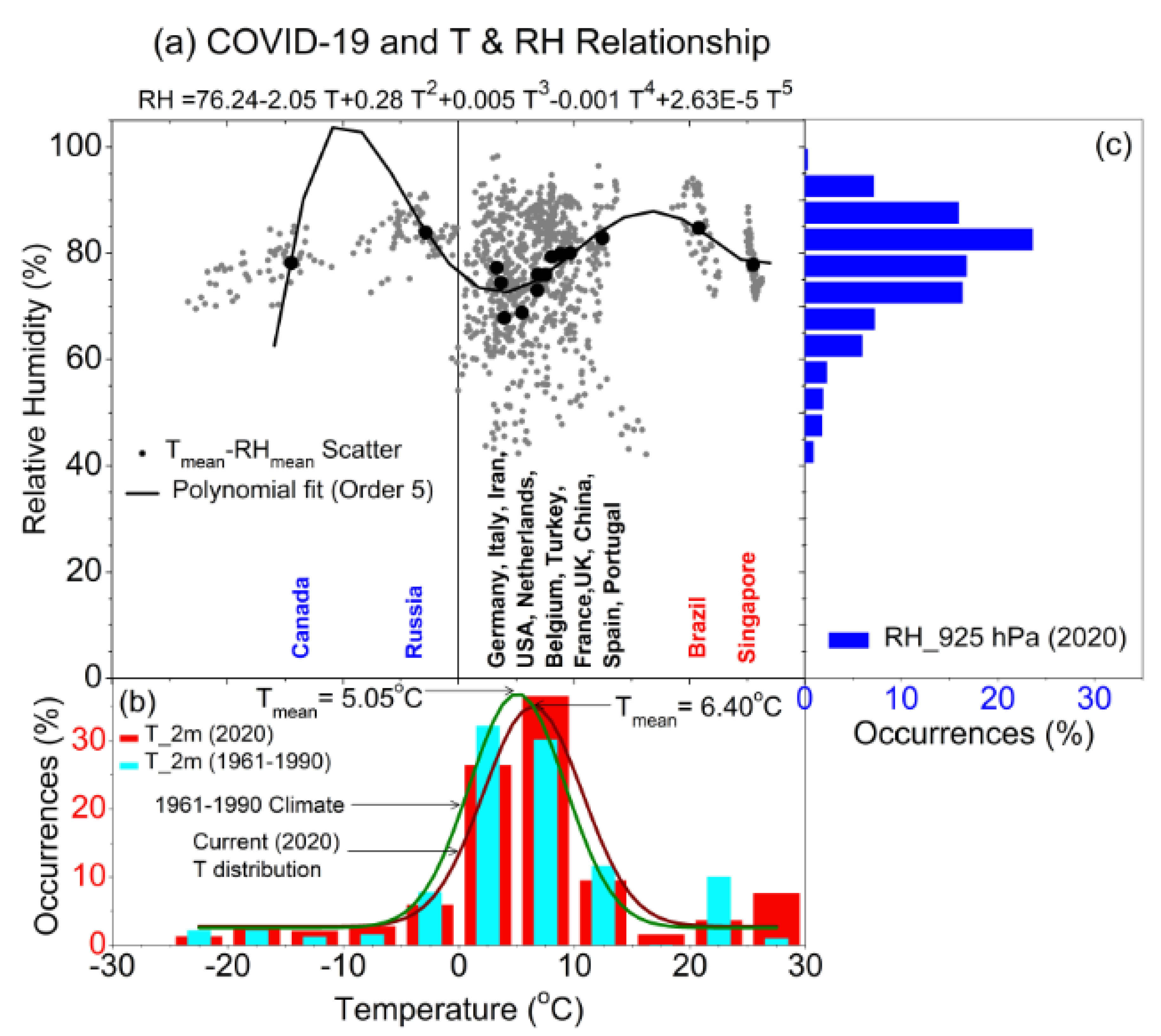
5. Ambient Temperature and Relative Humidity

In the environment, an infectious virus remains active on the contaminated surfaces; the duration of its persistence and transmission is affected by the external conditions, e.g., temperature and relative humidity [8]. For example, in tropical and temperate climates, humidity and temperature are the key indicators for predicting the influenza epidemics [43,44,45]. In the subtropical countries, the SARS Coronavirus remains active on smooth surfaces for ~5 days and facilitate community transmission at temperature and relative humidity between 22–25 °C and 40–50%, respectively [8]. In the present study, we investigate whether the climate variables, e.g., ambient temperature and relative humidity could be the factors in the survival and transmission of COVID-19.
For this study, we select 48 cities in 16 countries spread across 4 continents as epicenters (Table 1, Data and Methods). They include China, Iran, Singapore in Asia, Turkey, UK, Italy, Spain, Netherlands, Belgium, France, Portugal in Europe, Moscow in Russia, USA, and Canada in North America and Brazil in South America. Initially, the COVID-19 community transmission exhibits a consistent east to west pattern from Wuhan in China, Iran, Turkey, Europe, New York in USA, particularly above 25° N latitude (Figure 1). However, at the later stage (April–May) Brazil (Sao Paulo), Peru (Lima), Ecuador in South America and Singapore and India (Mumbai, Delhi) [20] in Asia also emerged as new COVID-19 hotspots [46,47].
The scatter diagram (gray dots) of NCEP Reanalysis (Data and Methods) T (2 m) and RH (925 hPa) and their mean values (black dots) are shown in Figure 2a; the top 10 vulnerable countries alongside USA and China are clustered between 0 °C and 10 °C (Figure 2b, histogram plot). A Gaussian fit on the histogram shows that Brazil and Singapore falls in the warmer side, whereas, Canada and Russia in the colder side of the spectrum. RH, on the other hand is clustered between 70–95% (Figure 2c, histogram plot). The scatter plot of daily COVID-19 counts as a function T and RH are shown in the right hand side of Figure 2b,c, respectively. Although, in the initial phase majority of the COVID-19 epicenters are clustered between 0–10 °C and above 25° N latitudes, there are emerging hotspots in the Southern Hemisphere (Brazil) and in the tropical region (Singapore) as well.
In general, seasonal respiratory diseases have a closer association with ambient temperature and humidity. We further analyze the changes in daily COVID-19 count as a function of T and RH for 16 epicenters in the Supplementary Figures S3–S8. During the entire evolution period (initial growth, faster growth, and decay), in most cases, daily COVID-19 counts vary quasi-linearly with T and RH, but in the opposite direction. In the growing phase, the near-linear covariability between T and daily COVID-19 counts is very prominent between 0 °C and 10 °C in USA, UK, Spain, Italy, France, Netherlands, China, Belgium, Portugal, and Turkey. The correlation coefficient is higher than 0.8 and in some cases, it exceeds 0.95, which can accounts at least 65–95% of the explained variance. It indicates that the spread and survival of SARS-CoV-2 in the environment depends on the complex interplay between T and RH. In the warmer (Singapore and Brazil) and colder (Russia and Canada) countries, T co-varies with the COVID-19 counts but in the higher (20 to 26 °C) and lower (−15 °C to 0 °C) temperature ranges, respectively. The RH, though, behaves similarly but in a less systematic fashion compare to T and remains above 70% throughout the growing phase. Most of the epicenters have experienced humid environmental conditions, which is due to the proximity of the epicenters (distance from the capital of the states/cities) to the larger water bodies like sea, ocean or lakes. It indicates that relative humidity in most of the epicenters is high, which may facilitate a favorable environment for the transmission of SARS-CoV-2. However, the topography of the regions needs to be considered as well, e.g., in California, which expands along the ocean, towns inside the land sometimes experience huge difference in relative humidity than the coastal towns at a short distance. In the decay phase, the daily count decreases as T increases beyond 10 °C and RH decreases below 70%, particularly in UK, Germany, Spain, Italy, France, Netherlands, China, Iran, Belgium, and Portugal. A stronger covariability between daily COVID-19 counts and T/RH in diverse environmental conditions (particularly temperature) indicates that SARS-Cov-2 possesses characteristics which are beyond seasonal in nature.
By screening 517 articles and reviewing 17 studies, Mecenas et al. (2020) [18] observed homogeneity in the findings regarding the effect of temperature and humidity on transmissibility of COVID-19. They concluded that “a warmer climate is less likely to spread the virus”, “wetter climate inhibits the virus spread” and “cold and dry conditions were potentiating factors on the spread of the virus”. In the current study, we observe that the epicenters are mostly clustered at temperatures within 0 °C–10 °C, however, at the later stage, COVID-19 counts are higher in the warmer (South Africa, Brazil, and India; Sasikumar et al., 2020 [20]) and colder (Russia, Canada) countries, as well. In addition, most of the epicenters are close to the large water bodies i.e., the regions with higher relative humidity. These results are partly contradictory to the previous findings, which is probably due to the higher capability of SARS-Cov-2 to adapt in diverse environmental conditions. Secondly, we observe that the increase in COVID-19 counts depend more on the environmental conditions at the initial stage of the outbreaks i.e., prior to the community transmission phase.
Due to the closer association between COVID-19 counts and environmental conditions, we introduce a combined profile of temperature and humidity by employing a best fit polynomial curve (order 5) on the mean (in each of the epicenters) T and RH distribution (Figure 2a), which is statistically significant for predicting the COVID-19 cases and modeling cities or countries based on the environmental factors. In addition, any prior knowledge of external environmental conditions is significant to assess the degree of vulnerability of specific countries in different time periods.

6. CO2 Emission, Global Warming and Climate Change

According to the Paris Agreement (IPCC, 2015), it is widely understood that limiting the surface air temperature rise below 2.0 °C and more specifically within 1.5 °C could significantly reduce the threat and impacts of climate change [48]. Under the present scenario (business-as-usual/RCP8.5), the current emissions are slightly higher than RCP8.5, and therefore significant reduction in emissions are needed to keep 2 °C as an achievable goal in the near term [49]. It is known that global warming induced heat stress has a significant impact on the release and transmission of the zoonotic diseases. Wittmann et al. (2001) [50] reported that a rise in temperature by 2 °C could increase the release of the bluetongue virus and spread of Culicoides imicola. Moreover, it was reported that changes in temperature extremes (14–18 °C at the lower end and 35–40 °C at the upper end) facilitate a faster transmission of infectious diseases [18].
It is evident from the Fossil Fuel Data Assimilation System (FFDAS) V2 (Version 2) data that global CO2 emissions (Kg C m2 yr−1) have increased rapidly between 1997 and 2015 over East Asia (China, Japan, South Korea), South Asia (India), with the eastern part of United States and Europe accounting the most to this rise (Figure 3a), whereas, CO2 emissions are much less over the African Continent. The global zoonotic disease outbreak hotspots (heat map), i.e., high risk regions are centered in Europe, USA, Asia and Latin America. The predicted occurrences of the infected diseases are centered in the tropical regions, North America, Asia, Central Africa, and South America (Allen et al., 2017) [51], which collocate on the CO2 emission hotspots. In our present analysis, emissions of the particulate matters can block the natural immune system of the hosts and make them vulnerable to the infections. Interestingly, the location of the COVID-19 epicenters (>10,000 counts) coincide with the emission hotspots, e.g., Wuhan in China, Singapore, Iran, Turkey, Europe, Moscow in Russia, New York and New Jersey in the eastern part of USA, Washington and California in the western part of USA, Quebec and Ontario, in Canada, Sao Paulo in Brazil, South Africa and Egypt in Africa, and so on. The emission levels are higher in the severe, high, and medium COVID-19 affected centers, which suggest a possible linkage between fossil fuel emissions and COVID-19 outbreaks.
On one hand, the regions with higher CO2 emissions are vulnerable to the COVID-19 infections, while on the other hand, the survival and transmission of the SARS-CoV-2 virus depends strongly on ambient temperature conditions. Therefore, it is essential to investigate the empirical relationship between climate change due to fossil fuel emissions and COVID-19 pandemic. The histogram is constructed with T (2 m) data over 16 epicenters for the current period (1 January–25 April 2020) and the historical time period (1 January–25 April but for the period 1961–1990) in Figure 2b. Gaussian distribution curves are fitted on the histograms and the mean of the distributions are located at 6.40 °C and 5.05 °C for the current and historical period, respectively. The current distribution mean has shifted by 1.35 °C from its historical mean value towards the hotter extreme.
To evaluate the shift in current mean and the corresponding extremes, in Figure 3b, we classify the hotter extreme into moderate hot (mean-75th percentile), severe hot (75th–90th percentile) and extreme hot (>90th percentile) events. The 75th and 90th percentile of the distribution and centered at 6.86 °C and 13.09 °C, respectively. The right-hand side of Figure 3b displays total COVID-19 counts as a function of temperature. The fitted Gaussian curve on COVID-19 count peaks at a temperature of 7.49 °C, which is 2.44 °C and 1.35 °C higher than the historical mean and current mean value, respectively. The mean value (50th percentile) of COVID-19 count distribution lies in the severe domain of the historical (1 January–25 April for the period of 1961–1990) temperature distribution curve. Approximately 75% of the COVID-19 cases are clustered at the severe-extreme domain of the historical T (2 m) spectrum. The results indicate a possible association of COVID-19 pandemic with extreme hot climate. A combined schematic diagram linking the socio-environmental and climatic conditions are shown in Figure 4.
The viruses have the capability to adapt in diverse environmental conditions, particularly at different temperature and humidity conditions. They can block the natural immune system of the hosts and make them vulnerable to the infections [52] (more in Supplementary Information 1). Burning fossil fuel significantly increases the CO2 emission, which causes the regional and global surface temperature to rise beyond 2.0 °C. A hotter planet may induce heat stress on the zoonotic species and increases the adaptability of the viruses in hotter climate and diverse environmental conditions. It may change the relationship among the host species, infectious agents and their interactions with the human beings’ immune systems. From the spatial distribution of COVID-19 transmission pattern, it is evident that SARS-CoV-2 can adapt in the diverse (warmer/colder) environmental conditions (Figure 2). In the beginning, COVID-19 infections are clustered to the regions which are beyond 25° N latitude and atmospheric temperature ranges within 0–10 °C. In the later stage, the transmission occurs in the warmer countries like Brazil and Peru in South America and Singapore in the tropical region. It is interesting to note that India, being the closest neighbor to China, Japan, and South Korea, has an ambient temperature which probably inhibits the COVID-19 to spread in the warmer environmental conditions. The spread of SARS-CoV-2 in the tropical regions is probably due to the unique quality of SARS-CoV-2 to adapt in diverse environmental conditions. The mean temperature (7.49 °C) at which the SARS-CoV-2 is active over the epicenters is 1.35 °C higher than the climatological mean value. Therefore, the COVID-19 pandemic can be understood as a probable outcome of extreme climate change.

7. Summary and Conclusions

The ongoing COVID-19 outbreak has emerged as a global pandemic and the epicenters (infections >10,000) are distributed in 48 cities (16 countries) across 4 continents. Apart from higher population density and international travel routes, at the initial stage of the outbreak, i.e., prior to the community transmission phase, the survival and growth of SARS-CoV-2 also has tighter association with ambient temperature and relative humidity. The activity of SARS-CoV-2 is higher at temperature ranges between 0 °C and 10 °C and humidity above 70%, which are due to proximity of the epicenters closer to water bodies, i.e., regions with higher relative humidity. However, SARS-CoV-2 has the capability to adapt in diverse environmental conditions e.g., colder (−15 °C) countries like Russia and Canada and warmer (25 °C) countries like Singapore and Brazil. The combined temperature and humidity spectrum is highly significant for predicting the COVID-19 cases and modeling cities based on the environmental conditions.
It is known that an increasing CO2 emission due to unprecedented fossil fuel burning is the root cause of regional and global warming. In the recent decades, the global mean temperature distribution has shifted towards the hotter extremes, which increases the occurrences of extreme events, globally. An extreme hotter climate may induce excessive heat stress on the zoonotic species, providing a suitable environment for the viruses to adapt to the newer climate as well. It could alter the relationship among the infectious agents, host species, and their interactions with the humans’ immune systems. In addition, coronaviruses like SARS-CoV-2 are highly sensitive to global warming and climate change, which is evident from the fact that epicenters are collocated on global CO2 emission hotspots. The daily COVID-19 count peaks at 7.49 °C which is 1.35 °C and 2.44 °C higher than the current (1 January–25 April 2020) and historical (1 January–25 April for the period 1961–1990) mean value, respectively. Approximately 75% of the COVID-19 cases are clustered in severe-extreme domain of historical temperature distribution spectrum. COVID-19 poses serious health risk to the global community, which is possibly an outcome of anthropogenic climate change due to greenhouse gas emission. Despite a stronger association of COVID-19 epicenters with local CO2 emission hotspots, a quantitative assessment is necessary with many more cases and for longer timescale. Therefore, strenuous mitigation measures to abate GHG emission and limiting warming further beyond is an urgent need to avoid such pandemics in the future.

8. Data

The daily and cumulative COVID-19 counts data available from https://covid19.who.int/ and https://coronavirus.jhu.edu/ (accessed on 25 April 2020). For daily air temperature (T) at 2 m and Relative Humidity (925 hPa) data, we used the NCEP Reanalysis product (https://psl.noaa.gov/data/timeseries/daily/ (accessed on 25 April 2020)) over the selected locations, spanning from 1 January to 11 April 2020 (peak date for worldwide COVID-19 counts). However, for analysis, we have chosen the date when the first confirm cased was reported in the individual cities. 2-m Temperature (2 m) is temperature at the height of 2 m above earth’s surface. Relative humidity (RH) at 925 hPa is the percentage of the maximum amount of water vapor that the atmosphere can hold at a given temperature (saturation). For daily climatology, we used the 30 years of NCEP data from 1961 to 1990.
The Global Population Density (2020) was available from Gridded Population of the World, Version 3 (GPWv3): Population Count Grid. Palisades, NY: NASA Socioeconomic Data and Applications Center (SEDAC). http://dx.doi.org/10.7927/H4639MPP (accessed on 1 May 2020). The Global annual PM2.5 Grids from MODIS, MISR and SeaWiFS Aerosol Optical Depth (AOD) were available from Global Annual PM2.5 Grids from MODIS, MISR and SeaWiFS Aerosol Optical Depth (AOD), 1998–2012. Palisades, NY: NASA Socioeconomic Data and Applications Center (SEDAC). http://dx.doi.org/10.7927/H4028PFS (accessed on 1 May 2020). Fossil Fuel Data Assimilation System (FFDAS) version 2.0 data is available from the Purdue University. It can be downloaded from https://ffdas.rc.nau.edu/Data.html (accessed on 28 April 2020).

9. Materials and Methods

For our study, we select the COVID-19 pandemic epicenters or cities exceeding the infection counts of 10,000 by April 25th, 2020. The 48 cities in 16 countries spread across 4 continents have satisfied the above criteria are tabulated in Table 1. They include China, Iran, Singapore in Asia, Turkey, UK, Italy, Spain, Netherlands, Belgium, France, Portugal in Europe, Moscow in Russia, USA, and Canada in North America and Brazil in South America. We have selected the initial period of the outbreak, i.e., prior to the period when almost none of the selected countries met the first peak of the disease transmission. It is the period when the transmission depends more on the background environmental conditions. Initially, the COVID-19 community transmission exhibits a consistent east to west pattern from Wuhan in China, Iran, Turkey, Europe, New York in USA, particularly above 25° N latitude (Figure 1). However, at the later stage (April–May) Brazil (Sao Paulo), Peru (Lima), Ecuador in South America and Singapore, India (Mumbai, Delhi) in Asia also emerge as new COVID-19 hotspots.
To evaluate the shift in current mean and the corresponding hot extremes, we classify the hotter extreme into moderate hot (mean–66th percentile), severe hot (66–90th percentile), extreme hot (90–95th percentile) and record breaking hot (>95th percentile) events. Then we calculate the 66th, 90th and 95th percentile value of the historical (1961–1990) temperature distribution and compare with current year (1 January–25 April 2020) distribution to estimate the increase in extreme events. We plotted the COVID-19 count distribution over 48 epicenters as a function surface temperature and fitted the Gaussian curve on COVID-19 count distribution.
We applied a 5-day smoothing on each variable (Temperature and Relative Humidity) to obtain the background environmental condition, considering the COVID-19 incubation period of ~5 days.

Supplementary Materials

The following are available online at https://www.mdpi.com/2071-1050/13/6/3029/s1, Figure S1: Global Population Density Grid, 2020 (upper panel), Worldwide distribution of Airports and Air Transport Traffic Statistics (bottom panel). The population density map is available from Socio-Economic Data and Applications Center (SEDAC), Worldwide Airport distribution map from https://www.partow.net/miscellaneous/airportdatabase/ (accessed on 1 May 2020) and Air Transport Traffic Statistics data from International Air Transport Association, 2019; Figure S2: Global annual PM2.5 data; Figure S3: USA, Canada and Russia. (Top Panel) Daily and Cumulative COVID-19 Counts as a function of time, (Middle Panel) Daily temperature and Relative Humidity as a function of time, (Bottom Panel) Daily COVID-19 Counts as function of temperature and Relative humidity; Figure S4: Same as Figure S3 but for UK, Germany and Spain; Figure S5: Same as Figure S3 but for Italy, France and Netherlands; Figure S6: Same as Figure S3 but for China, Iran and Singapore; Figure S7: Same as Figure S3 but for Belgium, Portugal and Turkey; Figure S8: Same as Figure S3 but for Brazil.

Author Contributions

D.N. has analyzed the data, interpret the results and written the manuscript, K.S. and R.N. performed data analysis; W.C. provided valuable suggestions and contributed in data interpretation. All authors have read and agreed to the published version of the manuscript.

Funding

This research received no external funding.

Institutional Review Board Statement

Not applicable.

Informed Consent Statement

Not applicable.

Competing Interest Statement

The authors declare that there are no competing interest.

Data Availability Statement

The daily and cumulative COVID-19 counts data is available from https://covid19.who.int/ and https://coronavirus.jhu.edu/ (accessed on 25 April 2020). The daily or cumulative COVID-19 data for different epicenters can be obtained by selecting them from the dashboard. The NCEP Reanalysis data is available from https://psl.noaa.gov/data/timeseries/daily/ (accessed on 25 April 2020). The users can select NCEP reanalysis data; input the latitude, longitude, month and year, the selected timeseries data can be downloaded for the epicenters. The Global Population Density (2020) was available from Gridded Population of the World, Version 3 (GPWv3): Population Count Grid. Palisades, NY: NASA Socioeconomic Data and Applications Center (SEDAC). https://sedac.ciesin.columbia.edu/ (accessed on 1 May 2020). The authors need to proceed to the Maps or Data section for downloading and can use them with proper citation. The Global annual PM2.5 Grids from MODIS, MISR and SeaWiFS Aerosol Optical Depth (AOD) were available from Global Annual PM2.5 Grids from MODIS, MISR and SeaWiFS Aerosol Optical Depth (AOD), 1998–2012. Palisades, NY: NASA Socioeconomic Data and Applications Center (SEDAC). https://sedac.ciesin.columbia.edu/ (accessed on 1 May 2020). The authors need to proceed to the Maps or Data section for downloading and can use them with proper citation. Fossil Fuel Data Assimilation System (FFDAS) version 2.0 data is available from the Purdue University. It can be downloaded from https://ffdas.rc.nau.edu/Data.html (accessed on 28 April 2020).

Code Availability Statement

The software codes related to the manuscript are available on request to the author.

Acknowledgments

The authors acknowledge the Physical Research Laboratory (PRL) for providing the daily NCEP Reanalysis data (https://psl.noaa.gov/data/timeseries/daily/) (accessed on 25 April 2020). For Global Population Density (2020) and Global annual PM2.5 Grids from MODIS, MISR and SeaWiFS Aerosol Optical Depth (AOD) the authors acknowledge NASA Socioeconomic Data and Applications Center (SEDAC). https://sedac.ciesin.columbia.edu/ (accessed on 1 May 2020). This work is supported jointly by the National Natural Science Foundation of China (Grant No. 41750110484, 41675061) and Ministry of Science and Technology of China (2016YFA0600604), Key Research Program of Frontier Sciences, CAS (QYZDY-SSW-DQC024).

Conflicts of Interest

The authors declare no conflict of interest.

References

  1. Center for Strategic and International Studies (CSIS) Report. 2020. Available online: https://www.csis.org/analysis/global-economic-impacts-covid-19 (accessed on 1 May 2020).
  2. She, J.; Jiang, J.; Ye, L.; Hu, L.; Bai, C.; Song, Y. 2019 novel coronavirus of pneumonia in Wuhan, China: Emerging attack and management strategies. Clin. Transl. Med. 2020, 9, 19. [Google Scholar] [CrossRef] [PubMed]
  3. Zhu, N.; Zhang, D.; Wang, W.; Li, X.; Yang, B.; Song, J.; Zhao, X.; Huang, B.; Shi, W.; Lu, R.; et al. A Novel Coronavirus from Patients with Pneumonia in China, 2019. N. Engl. J. Med. 2020, 382, 727–733. [Google Scholar] [CrossRef] [PubMed]
  4. Huang, C.; Wang, Y.; Li, X.; Ren, L.; Zhao, J.; Hu, Y.; Zhang, L.; Fan, G.; Xu, J.; Gu, X.; et al. Clinical features of patients infected with 2019 novel coronavirus in Wuhan, China. Lancet 2020, 395, 497–506. [Google Scholar] [CrossRef] [Green Version]
  5. Pneumonia of Unknown Cause—China. WHO Disease Outbreak News, 5 January 2020.
  6. WHO Situation Reports; WHO: Geneva, Switzerland, 2020; pp. 1–100.
  7. Liu, J.; Liao, X.; Qian, S.; Yuan, J.; Wang, F.; Liu, Y.; Wang, Z.; Wang, F.-S.; Liu, L.; Zhang, Z. Community Transmission of Severe Acute Respiratory Syndrome Coronavirus 2, Shenzhen, China, 2020. Emerg. Infect. Dis. 2020, 26. [Google Scholar] [CrossRef] [PubMed]
  8. Chan, J.F.-W.; Yuan, S.; Kok, K.-H.; To, K.K.-W.; Chu, H.; Yang, J.; Xing, F.; Liu, J.; Yip, C.C.-Y.; Poon, R.W.-S.; et al. A familial cluster of pneumonia associated with the 2019 novel coronavirus indicating person-to-person transmission: A study of a family cluster. Lancet 2020, 395, 514–523. [Google Scholar] [CrossRef] [Green Version]
  9. Li, Q.; Guan, X.; Wu, P.; Qun, L.; Xuhua, G.; Peng, W.; Xiaoye, W.; Lei, Z.; Yeqing, T.; Ruiqi, R.; et al. Early transmission dynamics in Wuhan, China, of Novel Coronavirus—Infected pneumonia. N. Engl. J. Med. 2020, 382, 1199–1207. [Google Scholar] [CrossRef] [PubMed]
  10. Burke, R.M.; Midgley, C.M.; Dratch, A.; Fenstersheib, M.; Haupt, T.; Holshue, M.; Ghinai, I.; Jarashow, M.C.; Lo, J.; McPherson, T.D.; et al. Active monitoring of persons exposed to patients with confirmed COVID-19—United States, January–February 2020. Morb. Mortal. Wkly. Rep. 2020, 69, 245. [Google Scholar] [CrossRef] [PubMed] [Green Version]
  11. World Health Organization. Report of the WHO-China Joint Mission on Coronavirus Disease 2019 (COVID-19) 16–24 February 2020; World Health Organization: Geneva, Switzerland, 2020; Available online: https://www.who.int/docs/default-source/coronaviruse/whochina-joint-mission-on-covid-19-final-report.pdf (accessed on 25 April 2020).
  12. WHO. Modes of Transmission of Virus Causing COVID-19: Implications for IPC Precaution Recommendations; WHO: Geneva, Switzerland, 2020. [Google Scholar]
  13. Wong, C.-M.; Thach, T.Q.; Chau, P.Y.K.; Chan, E.K.P.; Chung, R.Y.-N.; Ou, C.-Q.; Yang, L.; Peiris, J.S.M.; Thomas, G.N.; Lam, T.-H.; et al. Part 4. Interaction between air pollution and respiratory viruses: Time-series study of daily mortality and hospital admissions in Hong Kong. Res. Rep. (Health Eff. Institute) 2010, 154, 283–362. [Google Scholar]
  14. Silva, D.R.; Viana, V.P.; Müller, A.M.; Livi, F.P.; Dalcin, P.D.T.R. Respiratory viral infections and effects of meteorological parameters and air pollution in adults with respiratory symptoms admitted to the emergency room. Influ. Other Respir. Viruses 2014, 8, 42–52. [Google Scholar] [CrossRef] [PubMed]
  15. Weber, T.P.; Stilianakis, N.I. Inactivation of influenza A viruses in the environment and modes of transmission: A critical review. J. Infect. 2008, 57, 361–373. [Google Scholar] [CrossRef]
  16. Pyankov, O.V.; Bodnev, S.A.; Pyankova, O.G.; Agranovski, I.E. Survival of aerosolized coronavirus in the ambient air. J. Aerosol. Sci. 2018, 115, 158–163. [Google Scholar] [CrossRef] [PubMed]
  17. Chan, K.H.; Peiris, J.S.M.; Lam, S.Y.; Poon, L.L.M.; Yuen, K.Y.; Seto, W.H. The Effects of Temperature and Relative Humidity on the Viability of the SARS Coronavirus. Adv. Virol. 2011, 2011, 734690. [Google Scholar] [CrossRef] [PubMed]
  18. Mecenas, P.; da Rosa Moreira Bastos, R.T.; Rosario Vallinoto, A.C.; Normando, D. Effects of temperature and humidity on the spread of COVID-19: A systematic review. PLoS ONE 2020, 15, e0238339. [Google Scholar] [CrossRef]
  19. Oliveiros, B.; Caramelo, L.; Ferreira, N.C.; Caramelo, F. Role of Temperature and Humidity in the Modulation of the Doubling Time of COVID-19 Cases. 2020. Available online: https://www.medrxiv.org/content/10.1101/2020.03.05.20031872v1 (accessed on 28 April 2020).
  20. Sasikumar, K.; Nath, D.; Nath, R.; Chen, W. Impact of Extreme Hot Climate on COVID-19 Outbreak in India. GeoHealth 2020, 4, 000305. [Google Scholar] [CrossRef] [PubMed]
  21. Naicker, P.R. The impact of climate change and other factors on zoonotic diseases. Arch. Clin. Microbiol. 2011, 2. [Google Scholar]
  22. Pappas, G. Of mice and men: Defining, categorizing and understanding the significance of zoonotic infections. Clin. Microbiol. Infect. 2011, 17, 321–325. [Google Scholar] [CrossRef] [PubMed] [Green Version]
  23. Cutler, S.J.; Fooks, A.R.; Van Der Poel, W.H.M. Public Health Threat of New, Reemerging, and Neglected Zoonoses in the Industrialized World. Emerg. Infect. Dis. 2010, 16, 1–7. [Google Scholar] [CrossRef] [PubMed]
  24. Sachan, N.; Singh, V.P. Effect of climatic changes on the prevalence of zoonotic diseases. Vet. World 2010, 3, 519–522. [Google Scholar]
  25. Wang, L.-F.; Shi, Z.; Zhang, S.; Field, H.; Daszak, P.; Eaton, B.T. Review of Bats and SARS. Emerg. Infect. Dis. 2006, 12, 1834–1840. [Google Scholar] [CrossRef] [PubMed]
  26. Intergovernmental Panel on Climate Change (IPCC). Climate Change 2007: Synthesis Report—Summary for Policymakers. Available online: http://www.ipcc.ch/pdf/assessment-report/ar4/syr/ar4_syr_spm.pdf (accessed on 6 May 2010).
  27. Lacetera, N. Impact of climate change on animal health and welfare. Anim. Front. 2019, 9, 26–31. [Google Scholar] [CrossRef] [PubMed] [Green Version]
  28. Lancet, T. COVID-19: Too little, too late? Lancet 2020, 395, 755–838. [Google Scholar] [CrossRef]
  29. Socioeconomic Data and Applications Center (SEDAC). Gridded Population of the World (GPW), v3 2020. Available online: http://dx.doi.org/10.7927/H4639MPP (accessed on 1 May 2020).
  30. Colizza, V.; Barrat, A.; Barthélemy, M.; Vespignani, A. The role of the airline transportation network in the prediction and predictability of global epidemics. Proc. Natl. Acad. Sci. USA 2006, 103, 2015–2020. [Google Scholar] [CrossRef] [Green Version]
  31. The International Civil Aviation Organization (ICAO). Available online: https://www.icao.int/Security/COVID-19/Pages/default.aspx (accessed on 1 May 2020).
  32. The Global Airport Database. Available online: https://www.partow.net/miscellaneous/airportdatabase/ (accessed on 1 May 2020).
  33. IATA. International Air Transport Association Report; IATA: Montreal, QC, Canada, 2019. [Google Scholar]
  34. Bukhari, Q.; Jameel, Y. Will Coronavirus Pandemic Diminish by Summer? SSRN Electron. J. 2020. [Google Scholar] [CrossRef]
  35. Wong, T.W.; Lau, T.S.; Yu, T.S.; Neller, A.; Wong, S.L.; Tam, W.; Pang, S.W. Air pollution and hospital admissions for respiratory and cardiovascular diseases in Hong Kong. Occup. Environ. Med. 1999, 56, 679–683. [Google Scholar] [CrossRef] [PubMed] [Green Version]
  36. Ciencewicki, J.; Jaspers, I. Air Pollution and Respiratory Viral Infection. Inhal. Toxicol. 2007, 19, 1135–1146. [Google Scholar] [CrossRef] [PubMed]
  37. Zhu, Y.; Xie, J.; Huang, F.; Cao, L. Association between short-term exposure to air pollution and COVID-19 infection: Evidence from China. Sci. Total Environ. 2020, 727, 138704. [Google Scholar] [CrossRef] [PubMed]
  38. Fattorini, D.; Regoli, F. Role of the chronic air pollution levels in the Covid-19 outbreak risk in Italy. Environ. Pollut. 2020, 264, 114732. [Google Scholar] [CrossRef] [PubMed]
  39. Pansini, R.; Fornacca, D. Higher Virulence of COVID-19 in the Air-Polluted Regions of Eight Severely Affected Countries. Available online: https://www.medrxiv.org/content/101101/2020043020086496v2 (accessed on 1 May 2020).
  40. Pozzer, A.; Dominici, F.; Haines, A.; Witt, C.; Münzel, T.; Lelieveld, J. Regional and global contributions of air pollution to risk of death from COVID-19. Cardiovasc. Res. 2020, 116, 2247–2253. [Google Scholar] [CrossRef] [PubMed]
  41. van Donkelaar, A.; Martin, R.V.; Brauer, M.; Boys, B.L. Global Annual PM2.5 Grids from MODIS, MISR and SeaWiFS Aerosol Optical Depth (AOD), 1998–2012; NASA Socioeconomic Data and Applications Center (SEDAC): Palisades, NY, USA, 2015. [Google Scholar] [CrossRef]
  42. Peng, R.D.; Dominici, F.; Pastor-Barriuso, R.; Zeger, S.L.; Samet, J.M. Seasonal Analyses of Air Pollution and Mortality in 100 US Cities. Am. J. Epidemiol. 2005, 161, 585–594. [Google Scholar] [CrossRef] [PubMed]
  43. Bedford, T.; Riley, S.; Barr, I.G.; Broor, S.; Chadha, M.; Cox, N.J.; Daniels, R.S.; Gunasekaran, C.P.; Hurt, A.C.; Kelso, A.; et al. Global circulation patterns of seasonal influenza viruses vary with antigenic drift. Nat. Cell Biol. 2015, 523, 217–220. [Google Scholar] [CrossRef] [PubMed] [Green Version]
  44. Lemaitre, J.; Pasetto, D.; Perez-Saez, J.; Sciarra, C.; Wamala, J.F.; Rinaldo, A. Rainfall as a driver of epidemic cholera: Comparative model assessments of the effect of intra-seasonal precipitation events. Acta Trop. 2019, 190, 235–243. [Google Scholar] [CrossRef] [PubMed]
  45. Tamerius, J.D.; Shaman, J.; Alonso, W.J.; Bloom-Feshbach, K.; Uejio, C.K.; Comrie, A.; Viboud, C. Environmental Predictors of Seasonal Influenza Epidemics across Temperate and Tropical Climates. PLOS Pathog. 2013, 9, e1003194. [Google Scholar] [CrossRef]
  46. World Health Organization. WHO Coronavirus Disease (COVID-19) Dashboard. 2020. Available online: https://covid19.who.int/ (accessed on 3 March 2021).
  47. Johns Hopkins University (JHU). COVID-19 Dashboard. 2020. Available online: https://coronavirus.jhu.edu/ (accessed on 25 April 2020).
  48. King, A.D.; Karoly, D.J.; Henley, B.J. Australian climate extremes at 1.5 °C and 2 °C of global warming. Nat. Clim. Chang. 2017, 7, 412–416. [Google Scholar] [CrossRef]
  49. Vinke, K.; Schellnhuber, H.J.; Coumou, D.; Geiger, T.; Glanemann, N.; Huber, V.; Kropp, J.P.; Kriewald, S.; Lehmann, J.; Levermann, A.; et al. A Region at Risk: The Human Dimensions of Climate Change in Asia and the Pacific; Asian Development Bank (ADB): Mandaluyong, Philippines, 2017. [Google Scholar] [CrossRef] [Green Version]
  50. Rogelj, J.; Den Elzen, M.; Höhne, N.; Fransen, T.; Fekete, H.; Winkler, H.; Schaeffer, R.; Sha, F.; Riahi, K.; Meinshausen, M. Paris Agreement climate proposals need a boost to keep warming well below 2 °C. Nature 2011, 534, 631–639. [Google Scholar] [CrossRef] [Green Version]
  51. Wittmann, E.; Mellor, P.; Baylis, M. Using climate data to map the potential distribution of Culicoides imicola (Diptera: Ceratopogonidae) in Europe. Rev. Sci. Tech. Off. Int. Epizoot. 2001, 20, 731–740. [Google Scholar] [CrossRef]
  52. Allen, T.; Murray, K.A.; Zambrana-Torrelio, C.; Morse, S.S.; Rondinini, C.; Di Marco, M.; Breit, N.; Olival, K.J.; Daszak, P. Global hotspots and correlates of emerging zoonotic diseases. Nat. Commun. 2017, 8, 1124. [Google Scholar] [CrossRef] [PubMed]
Figure 1. Global distribution of the COVID-19 Pandemic (updated 25 April 2020). The color code indicates the severity of the event. The epicenters (infection count > 10,000) are marked with bigger dots. The higher the number of COVID-19 counts, the higher the severity is.
Sustainability 13 03029 g001
Figure 2. (a) Scatter plot (gray dots) T and RH in 48 cities across 16 countries. The right panel shows scatter plot (black dots) of Tmean and RHmean and polynomial fit of order 5 (black line), (b) (left panel) percentage of occurrences of T (2 m) and Gaussian fit during the current period (1 January–25 April 2020, red bar) and historical period (1 January–25 April but for the period of 1961–1990, cyan bar) as a function of T, (c) (left panel) percentage of occurrences of RH (925 hPa) and Gaussian fit during the current period (1 January–25 April 2020, blue bar) as a function of RH.
Sustainability 13 03029 g002
Figure 3. (a) Total Emissions (Kg C m2 yr−1) from FFDAS v2, average from 1997 and 2015, (b) Percentage of Occurrences of T(2m) as a function of T (left), Total COVID-19 Count distribution as a function of T (Gray bars) and Gaussian distribution on it (Black line).
Sustainability 13 03029 g003
Figure 4. Schematic Diagram. The background map represents the Population Density distribution over the globe. The socio-environmental (CO2 Emissions, International travels, Temperature & Relative humidity) and Climatic conditions (Global warming and Climate extremes) of the epicenters are shown above. The figures in red indicate cumulative COVID-19 counts. The bigger circle indicate COVID-19 counts higher than 500,000.
Sustainability 13 03029 g004
Table 1. List of COVID-19 Epicenters selected for the study.
Sr. No.ContinentCountryCity/StatesLatitude & LongitudeDistance from Waterbody (km)Cumulative Counts
1North AmericaUnited States of AmericaNew York40.71 N, 74 W2.4287,898
2New Jersey39.83 N, 74.87 W68.5105,198
3Michigan44.18 N, 84.5 W2538,789
4Massachusetts42.40 N, 71.38 W557,537
5Pennsylvania41.2 N, 77.19 W34441,153
6California36.77 N, 119.4 W20042,771
7Louisiana30.39 N, 92.32 W12095,058
8Illinois39.83 N, 89.64 W1041,777
9Florida27.66 N, 81.51 W7530,839
10Texas31.16N, 99.68 W50024,287
11Georgia33.24 N, 83.44 W20023,222
12Connecticut41.51 N, 72.66 W5024,583
13Washington47.75 N, 120.74 W25013,319
14Maryland38.95 N, 76.70 W10017,766
15Indiana39.91 N, 86.28 W20014,399
16Colorado38.99 N, 105.54 W100012,968
17CanadaQuebec53.21 N, 72.45 W30046,371
18EuropeItalyLombardy45.46 N, 9.18 E200195,351
19Emilia-Romagna44.49 N, 11.32 E100
20Piedmont45 N, 7.68 E100
21Veneto45.54 N, 11.55 E25
22GermanyBavaria48.13 N, 11.57 E250156,513
23North Rhine-Westphalia50.73 N, 7.09 E150
24Baden-Wurttemberg48.75 N, 8.24 E300
25SpainCatalonia41.35 N, 1.49 E75205,905
26Madrid40.25 N, 3.42 W250
27Castile-La Mancha39.85 N, 4.02 W200
28Castila Leon41.65 N, 4.72 W150
29Andalusia37.78 N, 3.78 W100
30Valencia39.46 N, 0.36 E5
31Galicia42.46 N, 7.24 E75
32Basque Country43.26 N, 2.92 W25
34FranceIle-de-France48.84 N, 2.63 E125161,647
35Alsace-Champagne-Ardenne-Lorraine48.79 N, 4.47 E300
36UKEngland51.30 N, 0.7 W100155,453
37NetherlandsNorth Brabant51.57 N, 4.76 E5037,384
38Amsterdam52.35 N, 5.00 W5
39BelgiumHasselt50.92 N, 5.33 E2045,325
40PortugalPorto41.14 N, 8.61 W323,392
41TurkeyIstanbul41.01 N, 28.97 E2107,773
42Izmir38.41 N, 27.12 E1
43Trabzon41.00 N, 39.71 E1
44RussiaMoscow City46.73 N, 117 W91574,588
45South AmericaBrazilSao Paulo23.55 S, 46.63 W50290,200
46AsiaChinaWuhan30.58 N, 114.26 E83283,909
47SingaporeSingapore1.22 N, 103.48 E1029,020
48IranTehran35.69 N, 51.42 E7589,328
Publisher’s Note: MDPI stays neutral with regard to jurisdictional claims in published maps and institutional affiliations.

