A Case Study of Tomato (Solanum lycopersicon var. Legend) Production and Water Productivity in Agrivoltaic Systems

Abstract

The challenge of meeting growing food and energy demand while also mitigating climate change drives the development and adoption of renewable technologies ad approaches. Agrivoltaic systems are an approach that allows for both agricultural and electrical production on the same land area. These systems have the potential to reduced water demand and increase the overall water productivity of certain crops. We observed the microclimate and growth characteristics of Tomato plants (Solanum lycopersicon var. Legend) grown within three locations on an Agrivoltaic field (control, interrow, and below panels) and with two different irrigation treatments (full and deficit). Total crop yield was highest in the control fully irrigated areas a, b (88.42 kg/row, 68.13 kg/row), and decreased as shading increased, row full irrigated areas a, b had 53.59 kg/row, 32.76 kg/row, panel full irrigated areas a, b had (33.61 kg/row, 21.64 kg/row). Water productivity in the interrow deficit treatments was 53.98 kg/m³ greater than the control deficit, and 24.21 kg/m³ greater than the panel deficit, respectively. These results indicate the potential of Agrivoltaic systems to improve water productivity even for crops that are traditionally considered shade-intolerant.

1. Introduction

Increasingly severe impacts of climate change and growing world populations provide an impetus for the development of renewable sources of energy which can supplement and replace fossil fuels. Implementation of large scale photovoltaic solar arrays is one step towards achieving this goal. In 2018, solar installations represented 22% of all new U.S. electric generation capacity [1]. In 2019, solar installation grew up 104% over 2018 [2]. At the end of 2018 global Photovoltaic capacity was 509 GW-DC and this capacity is expected to double by 2022 [1]. The increased capacity is in part a response to falling solar panel costs [3]. This increase in installed capacity requires large amounts of land and has led to competition over land that has traditionally been used for agriculture [4]. However, there is potential for solar installations and agricultural production to work together synergistically. Solar panels can provide electricity for different agricultural operations such as pumping irrigation water, operating post-harvest processing machines, etc. [5,6]. This dual use of land is often referred to as an Agrivoltaic System (AVS) or Agriphotovoltaic system. Agrivoltaic systems have been found to improve overall land use productivity by (60–70%) [7,8].

Solar and agriculture systems are formed Agrivoltaic systems when they present co-located in the same place to do mutual benefit [9]. They found crops which have less root density and high net photosynthetic rate considered ideal candidates.

Agrivoltaic systems have variations in application within agriculture to increase crop production beside electricity. For examples, the dual use solar panel–agriculture concept was first discussed in the literature by Goetzberger and Zastrow [10] who argued that when panels are lifted to a height of 2 m above the ground and spaced farther apart than traditional arrays, the system would receive approximately uniform solar radiation allowing for dual production. In the past decade multiple studies have been released which highlight potential to simultaneously spare land resources while increasing sustainable agriculture [6]. Some studies estimate up to a 70% increase in Land Use Efficiency using agrivoltaic systems [11]. Another study was used the multiple additive and synergistic benefits of Agrivoltic systems, including reduced plant drought stress and photovoltaic (PV) panel heat stress which can lead to improvements in crop yields [12]. Mean air temperature, relative humidity, wind speed, wind direction, and soil moisture were shown to be significantly different near panels as opposed to the control. Grass biomass and water use efficiency was significantly increased in the late season under PV panels (90% and 328%, respectively) [13]. Another study indicated that winter crops such as pea and wheat crops were benefited of solar shade less than summer crops [11].

One of the greatest potential synergies from these systems is the reduction in evaporative demand caused by the solar panel shading. This reduced water demand can lead to improvements in water use efficiency, here referring to the amount of yield (kg) produced by a given volume of water applied (m³). Marrou et al., found that on fields growing cucumber and lettuce, potential and soil water gradient were lower in the soil under the panels and led to an increase in harvested final fresh weight [14]. The rate of leaf canopy expansion was also found to be higher for cucumber and lettuce grown under the shade of solar panel, higher canopy cover is related to decreased evaporation [15]. Increasing water use efficiency was shown for agave plants that were co-located below solar panels [16]. Further work is needed to characterize the impact of Agrivoltaic systems on crop water productivity. In this paper, a field study was performed to measure the potential impact of Agrivoltaic system on tomato production and water productivity.

2. Material and Methods

2.1. Field Site

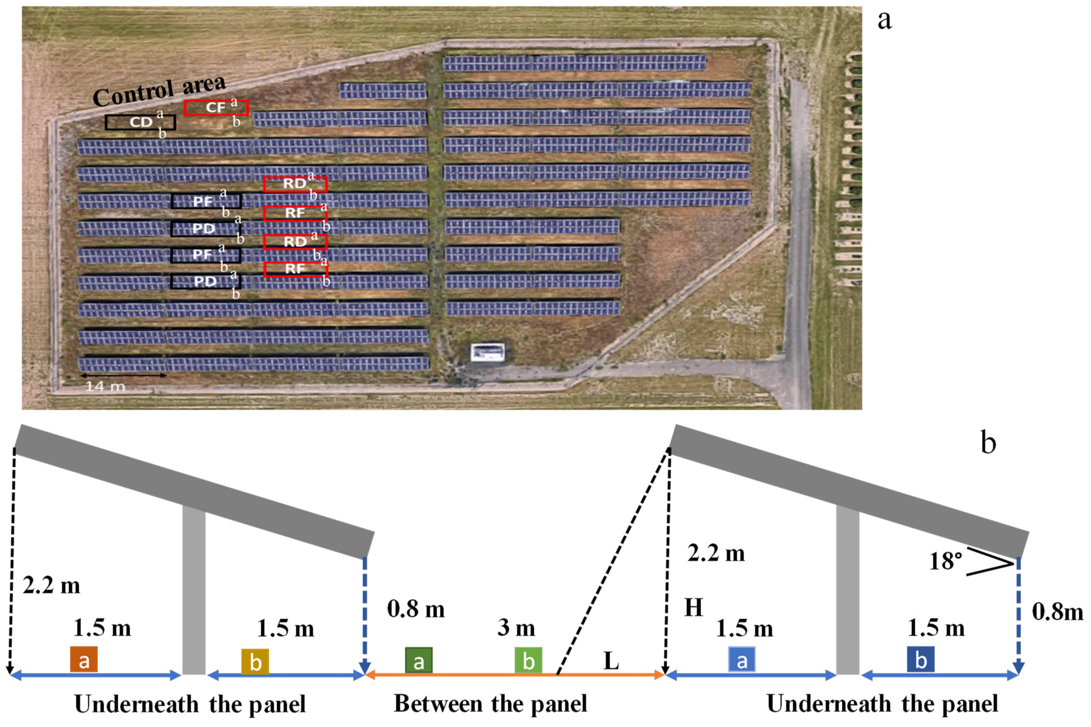
The field study was performed on a 0.8 ha solar array located on the Oregon State University Vegetable Farm (Corvallis, OR, USA). The Photovoltaic Panels (PVPs) have been arranged in east–west orientated strips, 3 m wide and inclined southward with a tilt angle of 18°. PVPs have been held at 0.8 m above ground at lowest point and 2.2 m above the ground at the highest point. The distance between panels is 3 m as shown in Figure 1. The solar array system has a total capacity of 482 kilowatts (http://fa.oregonstate.edu/sustainability/ground-mounted-photovoltaic-arrays (accessed on 15 February 2021)). As shown in Figure 1, the data were collected from localized zones (described hereafter) including areas below solar panels and a control area outside the agrivoltaic system. The site soil is Chehalis silty clay loam with a top soil pH of 6.23 and 6.06% organic matter content.

2.2. Site Preparation

Tomato transplants (Solanum lycopersicum var. Legend) were planted on 1st July 2019 in three light conditions: (1) directly beneath solar panels, (2) in rows between panels (3) in a control area located away from the panels (Referred to hereafter as “Panel”, “Row”, and “Control”, respectively) Figure 2. Each treatment was composed of two duplicated plots, with two rows of 20 plants in each plot. except for the control which only had a single plot for each irrigation treatment. Plants were placed in raised beds approximately 0.3 m above flat ground, two rows per bed. Spacing between rows was 1.5 m with 0.6 m between individual plants. Rows were covered with black plastic mulch. Two irrigation levels (Full and Deficit) were applied. Irrigation schedule was determined using the Management Allowable Depletion method. For the Full irrigation treatments, when the measured volumetric soil water content (SWC) reached 75% of the total available capacity the system was watered up to field capacity. For the deficit irrigation treatments, when the SWC reached 40% of total available capacity the system was watered until field capacity. Irrigation water was stored on site in (1.25017 m³) 275 gallon tanks, one tank per treatment. Water was applied using a drip system with one emitter per plant. Specifics regarding the irrigation design can be found in the next section. The fertilizer was applied (Wilco 16-16-16 northwest fertilizer) 2.15 kg per each row.

2.3. Irrigation Design Characteristics

2.3.1. Evaluate Pressure Compensating (PC) in Drip Irrigation

This study used 8 LPH (2GPH) Pressure compensating (PC) emitters (DIG company —model B222B, Vista, CA, USA). Emitter characteristics were evaluated using the catch can method. Irrigation was supplied via submersible pump (EcoPlous Eco 185 Fixed flow Submersible/inline pump ~600 L/h) one pump per treatment. During the catch can test, the irrigation system was run for 5 min at each treatment. The following parameters were described [17,18] and used to evaluate the PC drip irrigation operating:

2.3.2. Average Emitter Discharge Rate (q_a)

Computations of irrigation application followed the methodology. The average emitter discharge rate, q_a (m³/s), can be expressed as:

$${\mathrm{q}}_{\mathrm{a}}=\frac{1}{\mathrm{n}}{\displaystyle \sum }_{\mathrm{i}=1}^{\mathrm{n}}{\mathrm{q}}_{\mathrm{i}}$$

(1)

where

• $q_i$: the flow rate of the emitter i (m³/s)
• n: the total number of emitters.

2.3.3. Standard Deviation of Emitter Flow Rate (Sq)

The standard deviation of emitter flow rate, Sq, ASABE [19] can be written as:

$$S_q=\sqrt{\frac{1}{n-1}} {\displaystyle \sum }_{i=1}^n{( q_i-q_a)}^2$$

(2)

2.3.4. Uniformity Coefficient (UC)

The uniformity of water application (UC) is considering an important factor. Christiansen’s UC (%) evaluates the mean deviation, which is represented in ASABE standards as ASABE [19]:

$$UC=100 \left[1-\frac{1}{n{q}_a} {\displaystyle \sum }_{i=1}^n| q_i-q_a |\right]$$

(3)

2.3.5. Distribution uniformity (DU)

Low quarter distribution uniformity (DU) is used to all types of irrigation systems [20]. DU can be expressed as:

$$DU=100 \left(\frac{q_{m }}{q_{a }}\right)$$

(4)

where

• q_m: the average flow rate of the emitters in the lowest quartile.

2.4. Microclimatological Measurements

2.4.1. Climate Stations

Two weather stations were installed: one in the control area and one between the panel row the center of the solar panel area. Micrometeorological variables were collected data in 10-min intervals. The gathered variables were (1) air temperature (VP-3—Decagon Devices), (2) wind speed and direction (DS-2—Decagon Devices), (3) relative humidity (VP-3 -Decagon Devices) and (4) net radiation (PYR—Decagon Devices). Data were logged on EM50 data loggers (Decagon Devices). Reference ET was calculated from climate station in the control area and between the rows by using Penman-Monteith equation.

2.4.2. Arduino Array

In addition to the climate stations, an Arduino based climate sensor array was placed in the center of each treatment. The system measured (1) air temperature and (2) relative humidity (DHT22 -Adafruit industries), (3) Soil temperature (DS18B20 digital temperature sensor -Maxim Integrated products), and (4) Soil water content (SoilWatch 10—PINO-TECH).

Arduino arrays were situated in the center of each plot, 0.3 m above the ground. Soil temperature was measured at one point in the plot at a depth of 0.15 m. Soil moisture was measured at two points within the plot at a depth of 0.15 m. These data were collected from all sensors every 10 min. Soil moisture sensors were connected via relay to submersible pumps which controlled irrigation amounts via managed allowable depletion method.

Soil moisture content sensors were calibrated using field site soil samples with known volumetric water contents and comparison with other established soil moisture sensors (GS3—Decagon devices)

2.4.3. Evaporation during Measure Time

The evaporation was calculated during the season by using penman-Monteith equation. The equation parameters were measured such as temperature, wind speed and direction, and relative humidity.

$${\mathrm{ET}}_0=\frac{0408\Delta \left({\mathrm{R}}_{\mathrm{n}}-\mathrm{G}\right)+{\rm Y}\frac{900}{\mathrm{T}+273}{\mathrm{u}}_2\left({\mathrm{e}}_{\mathrm{s}}-{\mathrm{e}}_{\mathrm{a}}\right)}{\Delta +{\rm Y}\left(1+0.34{\mathrm{u}}_2\right)}$$

(5)

where:

• ET₀:—reference evapotranspiration [mm day^−1]
• R_n:—net radiation at the crop surface [MJ m⁻² day⁻¹]
• G:—soil heat flux density [MJ m⁻² day⁻¹]
• T:—mean daily air temperature at 2 m height [°C⁻¹]
• u₂:—wind speed at 2 m height [m s⁻¹]
• e_s:—saturation vapor pressure [kPa]
• e_a:—actual vapour pressure [kPa]
• e_s − e_a:—saturation vapour pressure deficit [kPa]
• ∆:—slope vapour pressure curve [kPa °C⁻¹]
• Υ:—psychrometric constant [kPa °C⁻¹]

2.4.4. Water Productivity

The actual water productivity was measured water applied to the crop during the season. Additionally, the crop yield was measured cumulative until end the season. WP actual can be expressed as:

WP-actual (kg ha⁻¹ m⁻³) = Ya/CWA

(6)

where, Ya is the actual yield (kg ha⁻¹), and CWA is the crop water availability (m³) measured during the season.

2.4.5. Biomass Measurements

The tomato biomass was collected at three points during the season. In total 46 plants were collected during each sampling period, six plants were collected from each plot, and three from each row. Plants were selected via random number generator. Harvested biomass was dried for 48 h in a 70 °C oven and weighed [21].

All tomatoes were harvested on a per row basis. A relatively large fraction of tomatoes did not ripen, likely due to the late planting date. This means that reported values may be inflated as there is always some fraction of tomatoes which will not ripen. This method still allows for comparison of relative yield between treatments.

3. Results and Discussion

3.1. Pressure Compensating Emitter Evaluation Characteristic

The most important parameters to characterize drip emitters and design of a drip irrigation system are average discharge rate (q_a) and standard deviation (S_q), Distribution Uniformity of water (DU), and Uniformity Coefficient (UC). Average emitter discharge rate distribution varied for all the treatments (Figure 3). This variability can be attributed to a combination of defects in individual emitters and tubing irregularity. Distribution uniformity (DU) is a measure of the uniformity of water application expressed as a percentage from (0–100%). The DU values below 70% are generally considered “poor” while values ranging from 70% to 90% are considered “good” and excellent greater than 90% (Rain Bird, 2008). Nine treatments have a DU value below 70%, and 4 treatment have a DU above 70% (Figure 3). DU plays a requisite role in determining the quantity of water required for irrigation and is dependent on many variables such as variation in the manufacturing of emitters, operating pressure heads, lateral lengths, and land slope. The UC results shown variations from 69.0% to 99.5%, (Figure 3). UC values were above 70% for all treatments except for row full.

3.2. Micrometeorological and Arduino Measurements

Results indicate that the presence of solar panels creates differences in the microclimate at a sub-field scale (Figure 4). Significant differences in mean air temperature were found between all treatments, except panel full and panel deficit which were not significantly different (p = 0.860) (Figure 4 and

Table 1. p-value for Air Temperature at variation treatment (Cells with value <0.00001 are left blank and 1 filled with grey color).

Treatment	Mean/Std	CD	CF	PD	PF	RD	RF	CS-C	CS-R
CD	22.26/8.39
CF	20.62/7.37						0.030
PD	19.80/5.65				0.860
PF	19.78/5.83			0.860
RD	21.52/8.15						0.002
RF	21.00/7.69		0.030			0.002
CS-C	17.98/7.16								0.019
CS-R	18.20/7.44							0.019

). Relative humidity values were not significantly different when comparing row full with control full (p = 0.207) and Row-Full with Panel-full (p = 0.563), but all other treatments were significantly different from each other (Figure 4 and

Table 2. p-value for Relative Humidity at variation treatment (Cells with value <0.00001 are left blank and 1 filled with grey color).

Treatment	Mean/Std	CD	CF	PD	PF	RD	RF	CS-C	CS-R
CD	70.12/26.45
CF	74.63/25.61				0.030		0.207
PD	72.66/21.30				0.002		0.002
PF	73.54/20.60		0.030	0.002			0.563
RD	79.38/24.53
RF	73.88/25.24		0.207	0.002	0.563
CS-C	0.77/0.21
CS-R	0.69/0.18

). No significant differences were found between average solar radiation at the two climate stations (p = 0.640), notably a climate station was not place directly under the panels where a significant difference in radiation would be assured. Average wind speeds at the climate stations were significantly different from each other (p < 0.05) (Figure 4). All treatments differed significantly in soil temperature except for control full and row deficit (Figure 4 and

Table 3. p-value for Soil Temperature at variation treatment (Cells with value <0.00001 are left blank and 1 filled with grey color).

Treatment	Mean/Std	CD	CF	PD	PF	RD	RF
CD	25.55/1.47
CF	24.53/1.18					0.934
PD	20.24/0.92
PF	19.81/0.94
RD	24.52/1.49		0.934
RF	24.75/2.76

). Mean volumetric water content differed significantly between all treatments (p < 0.026) (Figure 4 and

Table 4. p-value for Soil water content at variation treatment (Cells with value <0.00001 are left blank and 1 filled with grey color).

Treatment	Mean/Std	CD	CF	PD	PF	RD	RF
CD	0.34/0.02
CF	0.37/0.03
PD	0.36/0.03				0.027
PF	0.36/0.03			0.027
RD	0.31/0.02
RF	0.38/0.03

).

3.3. Reference ET

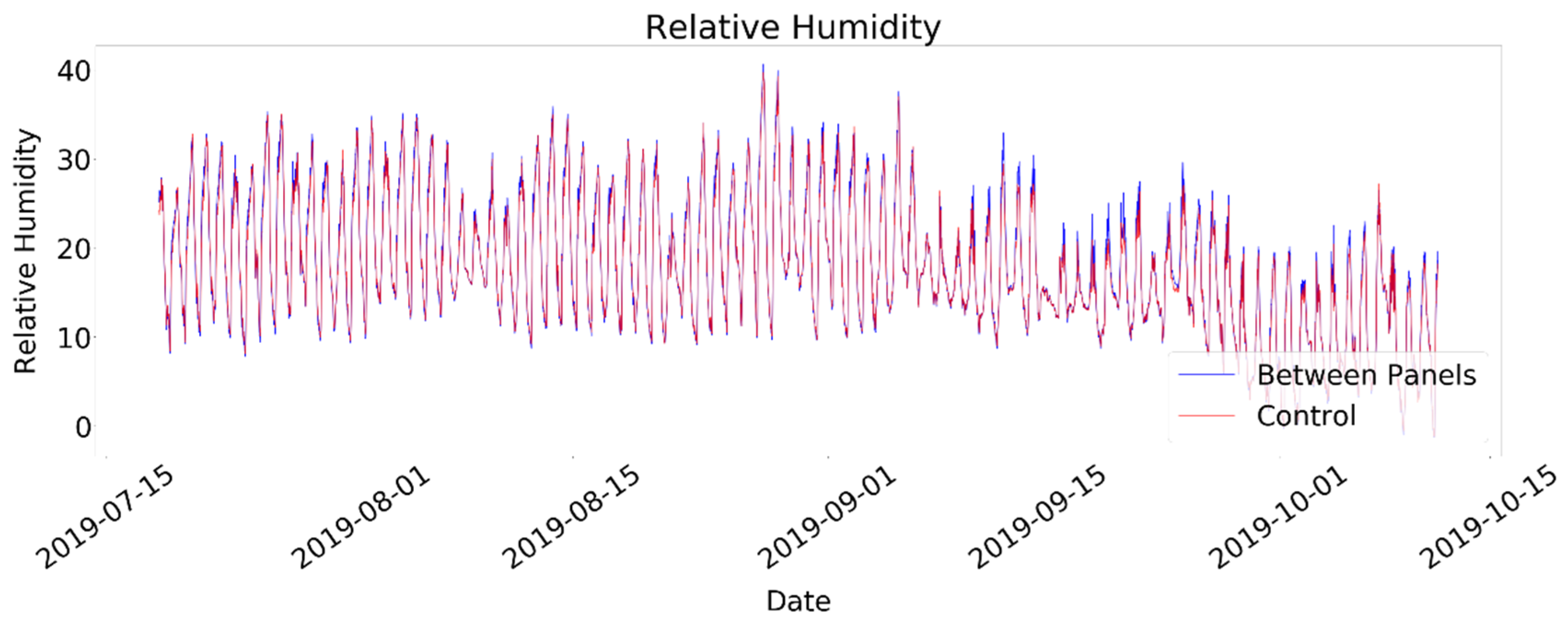
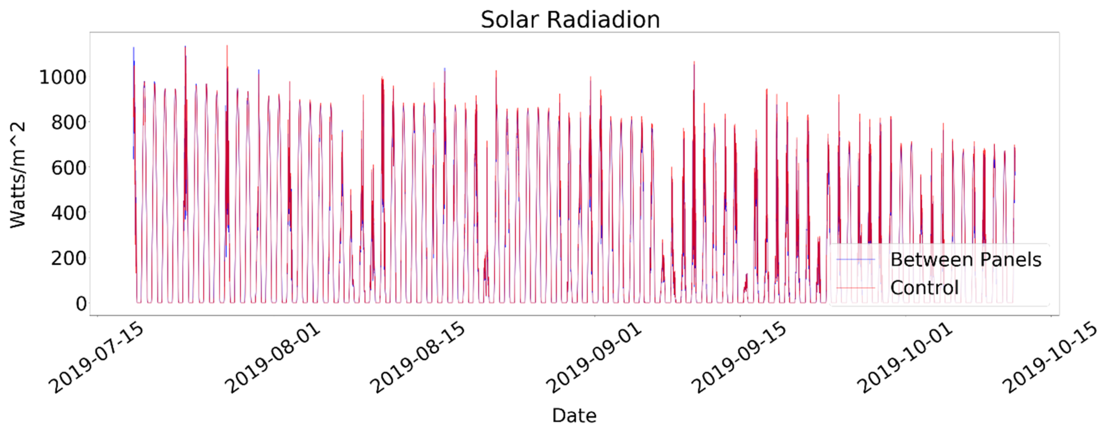
The reference ET was calculated using Penman-Monteith equation and climate station data, one station in the control area and one station between the rows of panels. The equation parameters were measured the relative humidity, solar radiation, and wind speed (Figure 5, Figure 6 and Figure 7), respectively. The results showed a significant between the control area and between panels for all the parameters.

A two tailed t-test showed a significant difference (p < 0.05) between control area and panel row (Figure 8). The reference (ETo)is higher in the control area compared to row plot area because control area has higher wind speed, radiation, and relative humidity that leads to increase ETo in control area.

3.4. Total Yield, Water Applied and Water Productivity

Total tomato yield was quantified by hand harvest on a per row basis, each row is 12.5 m × 3 m. Tomatoes were harvested every 2–3 days upon reaching maturity until the end of the season (October 10th). In the original experimental design, each plot was considered as a single treatment. As the season progressed it was noted that although the spacing between the rows was only 1.5 m, the individual rows showed large differences in growth characteristics. Rows that were less shaded demonstrated higher growth and thus considering both rows as a single treatment would not accurately represent the system. Rows within a treatment are identified as either “a” or “b” where a corresponds to the northern row and b corresponds to the southern. 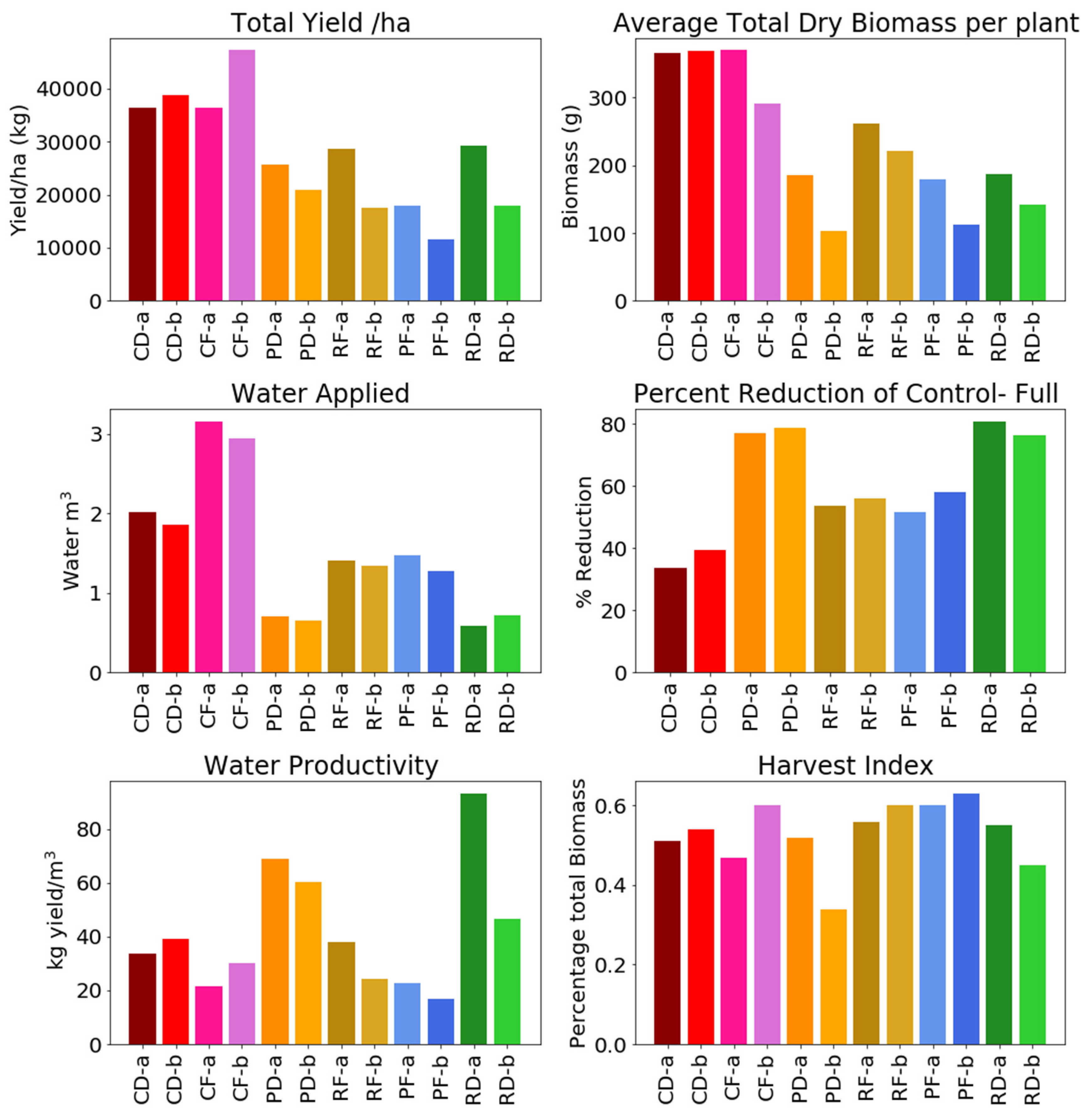Generally, the “a” rows showed higher yields, higher water demand, and greater water use productivity (Figure 9). These results emphasize the large amount of heterogeneity within agrivoltaic fields.

The total yield was highest in the control plots, both fully irrigated a, b (88.42 kg/row, 68.13 kg/row), and deficit a, b (72.54 kg/row, 68.30 kg/row) were higher than any of the treatments. If we scaled up to 1 ha these values correspond with ~47,160 kg/ha, ~36,340 kg/ha, and ~38,690 kg/ha, ~36,440 kg/ha. Row-full a and b and Row-deficit a and b compared to a panel full and deficit, respectively (Figure 9). The lowest yield showed in Panel-Full -b because it is interred row underneath the panel and get less sun light. The total yield result was expected yield scales directly with radiation.

Water applied was provided for each treatment from individual tank. Water applied was divided two irrigation level (deficit irrigation and full irrigation) distribution between control area; row and panel with two replicates. The results showed greater water applied to control full, control deficit compared to other treatments (Figure 9). The highest water applied showed in control-full-a and b, control deficit a and b (3.15 m³,2.94 m³, 2.02 m³, and 1.82 m³), respectively. The lowest water applied was in row deficit a, panel deficit b, panel deficit a, and row deficit b (0.59 m³, 0.65 m³, 0.70 m³, 0.72 m³), respectively. The percentage reduction showed highest water reduction above 80%, in row deficit, and more than 55% in panel deficit and row full compared to control full. These results agree with reference ET which showed high reference ET in the control area compared to row areas.

Water productivity was calculated as total yield divided by the total water applied to each treatment. The results showed increased water productivity in a panel full and deficit and row full and deficit compared to other treatments (Figure 9). The lowest water productivity showed in Panel-Full-b because it has less total yield and water applied is (1.28 m³). The water productivity showed higher in the row deficit a, panel deficit a and b (93.11 kg/m³, 68.90 kg/m³, and 60.31 kg/m³), respectively. These results suggest that deficit irrigation increased water productivity relative to the associated full irrigation across all treatments. Further, the deficit irrigated treatments within the solar array, both shaded and in the aisle, had approximately double the water productivity relative to the deficit irrigated control. We conclude that the shading effect of the solar array leads to additional water productivity beyond deficit irrigation alone.

3.5. Biomass and Harvesting Index

At the end of the season prior to yield harvesting, six tomato plants were randomly selected for total biomass analysis, three from each row. These samples were used to compute an average dry biomass. Yield was collected from each plant and then the plant was cut at the base of the stem and dried to determine total dry biomass. Tomato water content was measured to be 0.95, and this factor was used to calculate the dry yield from the total yield. A two tailed t-test showed statistically significant differences in biomass between all treatments (p < 0.01) as showed in Figure 9. Harvest index was calculated as the ratio of dry yield to total biomass. No significant differences were observed for harvest index, values ranged from 0.34 to 0.63.

4. Conclusions

Typical agricultural operations manage multiple on-farm resources including soil, nutrients and water. This study builds on the idea that on-farm solar resources can be managed in the same way that other natural resources are, and that a strategic partitioning of available solar radiation between crops and solar panels could be implemented for improvements in overall land use efficiency, solar energy production, and crop water productivity. Water limited areas are most likely to benefit from agrivoltaic systems as solar management reduces the reference evapotranspiration (ETo) and consequently the water demand. Many crop types may be managed beneath PV, but further economic analysis is needed to evaluate the costs and benefits of active solar management with PV panels.

Overall water productivity is also dependent on the characteristics of the chosen irrigation design. The emitter evaluation characteristics showed low average discharge rate and standard deviation in all the treatments. Uniformity coefficient and distribution uniformity were ranged 69—99.5% and 47—85%, respectively. Overall water productivity increases could potentially be more pronounced in systems with greater overall water distribution uniformity. The microclimate results showed significant differences in air temperature and relative humidity between all the treatments. Air temperature was highest in the control and row plots (22.3 °C, 21.5 °C), and lower beneath the panels (19.8 °C). Average relative humidity was highest in the row, followed by the control and then the panel areas (79.38%, 74.63%, 73.54%). In addition, soil temperature and soil moisture content showed significant difference among all the treatments. Increasing shading from panels corresponded with decreasing soil temperature. Average soil temperate was 20 °C in the panel area, 24.7 °C between the rows, and 25.6 °C in the control. When comparing wind speed data from the climate stations, speed was highest in control area compared to row area (0.89 m/s and 0.65 m/s). Reference ET was significantly different between the two stations in control area and between the row. Total crop yield was highest in the control full irrigated areas a, b (88.42 kg/row, 68.13 kg/row), and decreased as shading increased, row full irrigated areas a, b had 53.59 kg/row, 32.76 kg/row, panel full irrigated areas a, b had (33.61 kg/row, 21.64 kg/row). However, water applied was also highest in the control (a = 3.15 m³, b =2.94 m³). The combination of solar shading and deficit irrigation has the potential to trade a reduction in yields for reductions in water use. Water productivity was highest in areas which were both shaded and experiencing deficit irrigation, row deficit a (93.11 kg/m³) and panel deficit a (68.90 kg/m³). These results indicate the existence of some optimal water productivity point. While likely not the optimal point, the row deficit results demonstrate this potential, as the water row deficit water productivity is 53.98 kg/m³ greater than the control deficit, and 24.21 kg/m³ greater than the panel deficit. Finding this optimum is less important in a traditionally high-precipitation region like western Oregon but could be critical in areas which are currently water stressed and expect to become more water stressed in the coming years. Although total yield and water productivity varied between treatments, no significant difference was found in harvest index.

These results demonstrate the potential for water productivity improvements as a result of colocation of agricultural crops and photovoltaic solar arrays. However, more research is needed to determine how transferable these results are to different crops, different climatic regions, and to systems where panels are not ground mounted but are raised 3–5 m above the ground to allow for the use of traditional agricultural machinery. Growing resource scarcity dictates that improvements are needed in overall land use efficiency, Agrivoltaic systems may present a “win-win” scenario.

References

- NREL. Best Research-Cell Efficiencies; National Renewable Energy Laboratory: Golden, CO, USA, 2019. [Google Scholar]
- EUROPE, Solar Power. Global market outlook for solar power/2019–2023. 2019. Available online: https://www.solarpowereurope.org/wp-content/uploads/2019/07/SolarPower-Europe_Global-Market-Outlook-2019-2023.pdf (accessed on 15 February 2021).
- Trancik, J.E. Renewable energy: Back the renewables boom. Nat. News 2014, 507, 300. [Google Scholar] [CrossRef] [PubMed]
- Nonhebel, S. Renewable energy and food supply: Will there be enough land? Renew. Sustain. Energy Rev. 2005, 9, 191–201. [Google Scholar] [CrossRef]
- Santra, P.; Pande, P.C.; Kumar, S.; Mishra, D.; Singh, R.K. Agri-voltaics or solar farming: The concept of integrating solar PV based electricity generation and crop production in a single land use system. Int. J. Renew. Energy Res. 2017, 7, 694–699. [Google Scholar]
- Weselek, A.; Ehmann, A.; Zikeli, S.; Lewandowski, I.; Schindele, S.; Högy, P. Agrophotovoltaic systems: Applications, challenges, and opportunities. A review. Agron. Sustain. Dev. 2019, 39, 35. [Google Scholar] [CrossRef]
- Dupraz, C.; Marrou, H.; Talbot, G.; Dufour, L.; Nogier, A.; Ferard, Y. Combining solar photovoltaic panels and food crops for optimising land use: Towards new agrivoltaic schemes. Renew. Energy 2011, 36, 2725–2732. [Google Scholar] [CrossRef]
- Dinesh, H.; Pearce, J.M. The potential of agrivoltaic systems. Renew. Sustain. Energy Rev. 2016, 54, 299–308. [Google Scholar] [CrossRef]
- Seidlova, L.; Verlinden, M.; Gloser, J.; Milbau, A.; Nijs, I. Which plant traits promote growth in the low-light regimes of vegetation gaps? Plant Ecol. 2009, 200, 303–318. [Google Scholar] [CrossRef]
- Goetzberger, A.; Zastrow, A. New proposal by Fraunhofer-Gesellschaft. Potatoes under the collector. Sonnenergie 1981, 6, 19–22. [Google Scholar]
- Dupraz, C.; Talbot, G.; Marrou, H.; Wery, J.; Roux, S.; Liagre, F.; Clichy, D. To mix or not to mix: Evidences for the unexpected high productivity of new complex agrivoltaic and agroforestry systems. In Proceedings of the 5th World Congress of Conservation Agriculture: Resilient Food Systems for a Changing World, Brisbane, Australia, 26–29 September 2011. [Google Scholar]
- Barron-Gafford, G.A.; Pavao-Zuckerman, M.A.; Minor, R.L.; Sutter, L.F.; Barnett-Moreno, I.; Blackett, D.T.; Macknick, J.E. Agrivoltaics provide mutual benefits across the food–energy–water nexus in drylands. Nat. Sustain. 2019, 2, 848–855. [Google Scholar] [CrossRef]
- Adeh, E.H.; Selker, J.S.; Higgins, C.W. Remarkable agrivoltaic influence on soil moisture, micrometeorology and water-use efficiency. PLoS ONE 2018, 13, e0203256. [Google Scholar]
- Marrou, H.; Dufour, L.; Wery, J. How does a shelter of solar panels influence water flows in a soil–crop system? Eur. J. Agron. 2013, 50, 38–51. [Google Scholar] [CrossRef]
- Marrou, H.; Wéry, J.; Dufour, L.; Dupraz, C. Productivity and radiation use efficiency of lettuces grown in the partial shade of photovoltaic panels. Eur. J. Agron. 2013, 44, 54–66. [Google Scholar] [CrossRef]
- Ravi, S.; Lobell, D.B.; Field, C.B. Tradeoffs and synergies between biofuel production and large solar infrastructure in deserts. Environ. Sci. Technol. 2014, 48, 3021–3030. [Google Scholar] [CrossRef] [PubMed]
- Keller, J.; Bliesner, R.D. Sprinkle and Trickle Irrigation; Van Nostrand Reinhold: New York, NY, USA, 1990. [Google Scholar]
- Kang, Y.; Nishiyama, S. Analysis of microirrigation systems using a lateral discharge equation. Trans. ASAE 1996, 39, 921–929. [Google Scholar] [CrossRef]
- Schneider, A. Efficiency and uniformity of the lepaand spray sprinkler methods: A review. Trans. ASAE 2000, 43, 937. [Google Scholar] [CrossRef]
- Merriam, J.L.; Keller, J. Farm irrigation system evaluation: A guide for management. Farm Irrig. Syst. Eval. Guid. Manag. 1978. [Google Scholar]
- Patanè, C.; Tringali, S.; Sortino, O. Effects of deficit irrigation on biomass, yield, water productivity and fruit quality of processing tomato under semi-arid Mediterranean climate conditions. Sci. Hortic. 2011, 129, 590–596. [Google Scholar] [CrossRef]
Figure 1.
(a) Site map shows treatments distribution in the site, (b) Schematic drawing of shade zones (H is object height and L is shadow length.
Figure 2.
(a–c) The treatments beneath panel and (d–f) between Row in different plant stage.
Figure 3.
Emitter characterization of pressure compensating dripper for drip irrigation system: average emitter discharge rate and standard deviation; and UC, Christiansen’s uniformity coefficient and DU, Low quarter distribution uniformity.
Figure 4.
The mean value for all variables measured by microclimate station and Arduino array under two irrigation conditions (full and deficit) with three different areas (open area (control area), between solar panel and beneath the panel). Notice: CS-C = Climate station in the control area, and CS-R = Climate station in the Panel Row area.
Figure 5.
Impacts of colocation the relative humidity from beneath solar PV panels (agrivoltaic system), between the panel and control area and two climate station (between the panel and control area) on different irrigation treatment.
Figure 6.
Micrometeorological impacts of colocation of agriculture (agrivoltaic system) between the row and control area for solar radiation.
Figure 7.
Micrometeorological impacts of colocation of agriculture (agrivoltaic system) between the row and control area installations.
Figure 8.
Reference ET calculated for two weather station (between panel row and control area).
Figure 9.
Calculated total yield; water applied; water productivity; average total biomass per plant and harvest index for treatments under two irrigation conditions (full and deficit) with three different areas (open area (control area), between solar panel and beneath the panel) with two replicates for each area. Notices. CD: Control deficit a, b; CF: Control Full a, b; Panel Deficit a, b; RF: Row Full a, b; PF: Panel Full a, b and RD: Row Deficit a, b.