Article

Life Cycle Assessment of Households in Santiago, Chile: Environmental Hotspots and Policy Analysis

by
Camila López-Eccher
1,
Elizabeth Garrido-Ramírez
2,
Iván Franchi-Arzola
2 and
Edmundo Muñoz
2,*
1
School of Environmental Sciences and Sustainability, Universidad Andres Bello, Santiago 8370251, Chile
2
Center for Sustainability Research, Universidad Andrés Bello, Santiago 8370251, Chile
*
Author to whom correspondence should be addressed.
Sustainability 2021, 13(5), 2525; https://doi.org/10.3390/su13052525
Submission received: 5 February 2021 / Revised: 21 February 2021 / Accepted: 23 February 2021 / Published: 26 February 2021
(This article belongs to the Special Issue Life Cycle Management for Sustainable Regional Development)

Abstract

:
The aim of this study is to assess the environmental impacts of household life cycles in Santiago, Chile, by household income level. The assessment considered scenarios associated with environmental policies. The life cycle assessment was cradle-to-grave, and the functional unit considered all the materials and energy required to meet an inhabitant’s needs for one year (1 inh/year). Using SimaPro 9.1 software, the Recipe Midpoint (H) methodology was used. The impact categories selected were global warming, fine particulate matter formation, terrestrial acidification, freshwater eutrophication, freshwater ecotoxicity, mineral resource scarcity, and fossil resource scarcity. The inventory was carried out through the application of 300 household surveys and secondary information. The main environmental sources of households were determined to be food consumption, transport, and electricity. Food consumption is the main source, responsible for 33% of the environmental impacts on global warming, 69% on terrestrial acidification, and 29% on freshwater eutrophication. The second most crucial environmental hotspot is private transport, whose contribution to environmental impact increases as household income rises, while public transport impact increases in the opposite direction. In this sense, both positive and negative environmental effects can be generated by policies. Therefore, life-cycle environmental impacts, the synergy between policies, and households’ socio-economic characteristics must be considered in public policy planning and consumer decisions.

1. Introduction

Urban areas are considered the home of prosperity and development and large consumers of resources, which generate pollution, unsustainable growth, and social inequality [1]. Urban areas are responsible for 75% of the planet’s resource and energy consumption and 80% of global CO2 emissions [2]. This situation will worsen, considering that today around 50% of all inhabitants live in cities [3], and estimates indicate that this number will reach 68% by 2050 [4]. Thus, there is an increasing focus on consumption as an essential driver of social metabolism [5]. It has also shifted the focus to consider the requirements associated with the final sector demand, including that of households [6]. Beginning in the 1990s, older approaches evolved to take into account consumption [7], and new approaches appeared, such as integrated production or sustainable consumption and production policies [8,9], with particular focus on household consumption [7].
A household is defined as a group of persons who share the same living accommodation, pool some, or all, of their income and wealth, and consume certain types of goods and services collectively [6,7]. Households are significant drivers of the economy. Their consumption behavior triggers many economic activities along the supply chain of each product and service, which subsequently involves using resources and the release of emissions [10]. For this reason, the household might be regarded as ultimately responsible for environmental impacts occurring over the life cycle of products and services [10].
Many studies have focused on the resource consumption and environmental impacts of households. According to Matuštík and Kočí [11], personal consumption is among the most significant contributors affecting the global environment. Newton and Meyer [12] studied urban resource consumption such as water, energy, domestic appliances, and transport before concluding that it is more affected by contextual factors (household, dwelling and location) than individual ones (structural and attitudinal). Similarly, Froemelt et al. [10] assessed household consumption behavior. However, they focused their attention on assessing environmental impacts, proposing new approaches to determine their variability. The application of this approach demonstrates that within similar socioeconomic household types, different archetypes can be found. The proposed approach could lead to a better understanding of consumption patterns and the future support of environmental policymakers targeting specific consumer groups. In this sense, understanding the variability of consumption patterns and associated environmental impacts is required to devise targeted environmental policies [10]. Kalbar et al. [13] analyzed how urban lifestyles impact the environment. They applied a life cycle assessment approach coupled with personal metabolism, which determined that demographic parameters such as income level and respondent age strongly influence environmental impacts. Diet choices, private car use, and household size also significantly influence consumption-related environmental impacts.
Impacts associated with household consumption are generally calculated through environmental footprints, often pressure-based [14]. Examples include the carbon footprint [15,16], water footprint [17], land footprint [18], and material footprint [19]. All these indicators take a consumption-based approach, i.e., they consider the full life cycle of products and allocate impacts to the final consumer [14]. Life cycle assessment is one of the most widely used tools to assess household consumption’s environmental impacts. In this sense, life cycle thinking and assessment have emerged as crucial approaches to pave the way towards sustainable consumption and production [14]. Several studies implement top-down methodologies to make a general assessment of the impacts of household consumption, such as the environmentally extended input–output model (EIO-LCA) [20], environmentally extended, multi-regional input–output (EE-MRIO) tables [14], among other combinations of LCA and input–output analysis. Alongside this, regional and national statistics and censuses have been widely used to model household consumption [21,22,23].
Top-down methods have the advantage of providing a coherent framework for the allocation of environmental burdens and resource consumption generated by macro-level economic systems. However, they lack product-level detail [14] and do not allow for site-specific analyses associated with households’ socio-economic level and geographical location at the local level. On the other hand, other studies follow a bottom-up approach, based on the LCA of representative products, which are then up-scaled to overall consumption [24]. At the bottom-up level, it is possible to analyze specific geographical locations. Azimi et al. [25] through a survey questionnaire, examined the social impacts of the life cycle of the city of Kabul in Afghanistan. With the ultimate aim of supporting e-waste management in Vietnam [26], 1003 households in Hanoi and Hochiminh’s urban areas, the two biggest cities in Vietnam, were surveyed. Leray et al. [27] conducted research based on a pilot survey conducted in the city of Bangalore, India. The study considered six households whose socio-economic status was representative of India’s new urban middle classes. The results revealed a complex system of interactions between food supply, storage and management practices, and socio-cultural norms. In general, most bottom-up studies identify households’ metabolism and their consumption practices, revealing the types of consumption and the patterns and behaviors that generate them. They also commonly propose actions for environmental policies applicable to urban areas. However, few studies have modeled future management scenarios in urban areas or assessed the effect these strategies might have on households’ environmental impacts.
This study was devised to assess households’ life-cycle environmental impacts in Santiago, Chile, by household income level. In this way, the study sought to identify environmental hotspots and model future management scenarios associated with environmental policies. From the research analysis approach, it was possible to establish the main environmental benefits and adverse effects of decision-making, both those associated at the household level and those applicable at the national or urban level, through public policies.

2. Materials and Methods
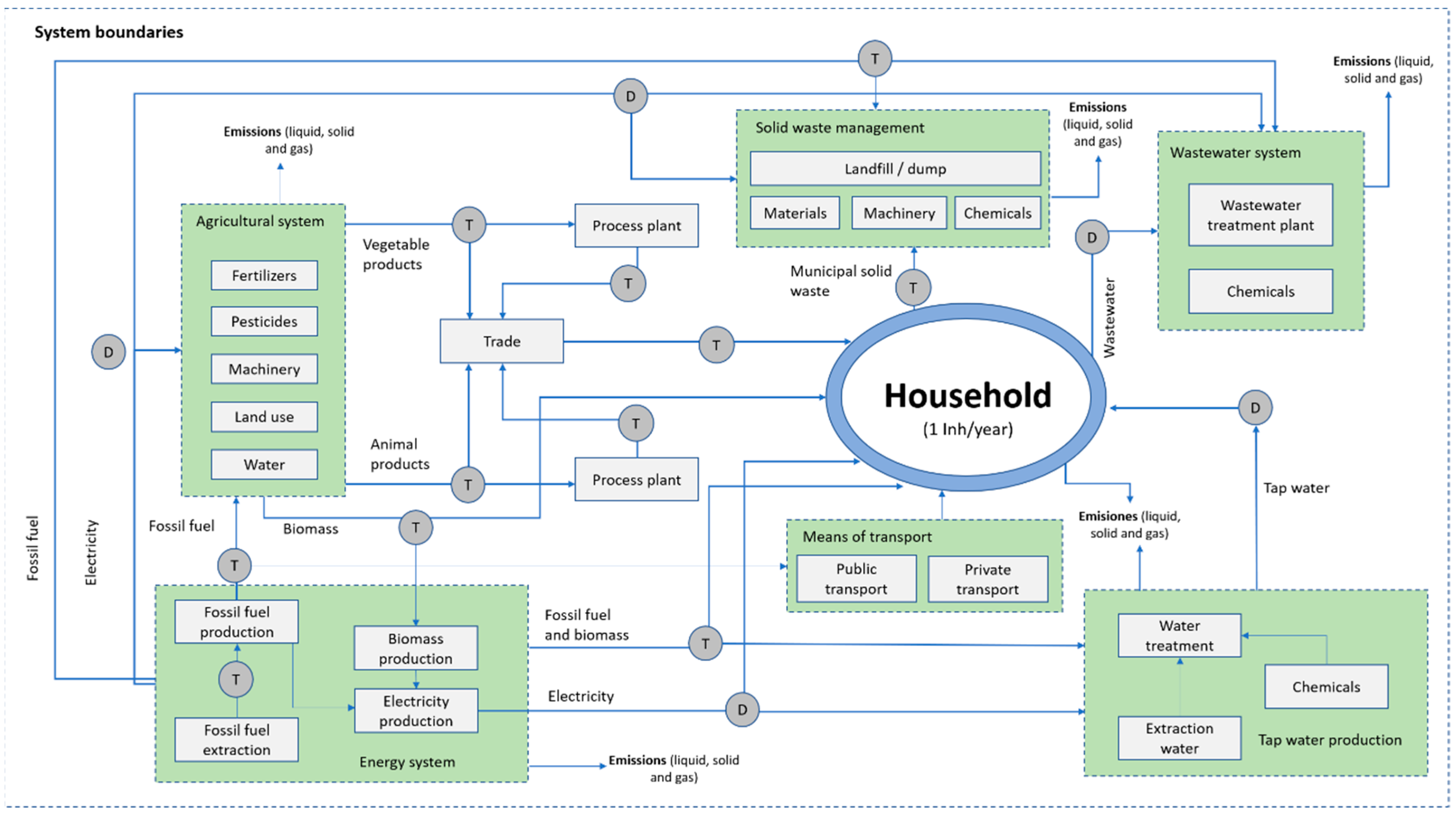
2.1. Goal and Scope

The objective of this study was to assess the environmental impacts of households in the city of Santiago, Chile, associated with different levels of household income. For this purpose, the life cycle assessment methodology was applied according to the requirements established by the ISO 14,040 standard [28]. The functional unit (FU), defined as the quantified performance of a system for use as a reference unit [29], was 1 inhabitant/year, which represents the consumption of a single individual in one year [11,23]. The study’s scope considered a cradle-to-grave approach, i.e., from the extraction of raw materials to the end of a product’s life. In this sense, the product system analyzed the extraction of raw materials and fossil fuels, food production and processing, energy production, transport, waste management and disposal, drinking water production and distribution, domestic wastewater collection and treatment. Figure 1 presents the product system used to carry out the household life cycle assessment.

2.2. Life Cycle Inventory

This study used a bottom-up methodology by conducting 300 household surveys in the city of Santiago. This information was complemented with secondary data from scientific articles, commercial databases, and national statistics. The surveys were conducted in three districts of Santiago with different socioeconomic characteristics. The selected districts were Providencia, Macul, and Pedro Aguirre Cerda, representing high, medium, and low socioeconomic levels, respectively. In each district, 100 randomly distributed surveys were conducted, which ensured a sample with different socioeconomic levels in Santiago. To obtain the sample, we used a shape of the urban property division for each district, which was obtained from the Chilean Internal Revenue Service [30]. The urban properties associated with a property roll number were selected randomly and then joined and distributed spatially through the ArcGIS 10.3 program. From this, a sample was generated and distributed throughout all macro sectors of Santiago.
The survey included 10 items and 63 questions, which were asked in the field using QuestionPro software. The items considered were: respondent and family group profile, household income, conditions and habitability, fuel consumption, household solid waste, environmental aspects, green areas, public transport, health system, and food. In the case of food, the information included in the Chilean Ministry of Social Development’s basic family basket was considered. The basic basket considers a threshold of 2000 average daily calories per person and was based on Chile’s VII Family Budget Survey [31]. In this sense, the categories included meats (beef, poultry and pork), fruits, vegetables, legumes, dairy products (yogurt, cheese, milk and butter, margarine), processed vegetable products (bread, flour, rice, oil, sugar, tea and coffee) and eggs. For the consumption of water, electricity, and natural gas, utility bills that contained the last 12 months’ consumption were requested.
Electricity was modeled using SimaPro 9.1 software, considering the National Electricity System (SEN) matrix for 2019, according to Muñoz et al. [32]. The SEN generation for 2019 was 36.8% coal, 26.9% hydroelectric, 18.3% natural gas, 8.2% photovoltaic, 6.2% wind, 2.4% biomass, 0.8% oil and 0.4% geothermal [33].
Public transport (bus and subway) is considered the time elapsed from home to destination (work, school, university, shopping, among others). For the transformation of minutes to kilometers traveled, average speeds were used, 45 km/h for the subway [34] and 14.3 km/h for buses [35]. The survey considered the average monthly consumption of gasoline and diesel fuel used by vehicles in each household for private transport.
Through SimaPro, the Ecoinvent 3.6 databases for vehicles and buses were used. From the same database, food, fuel, water, landfill, wastewater treatment, and subway systems were adapted to local conditions. Due to the non-existence of life cycle approach databases in Chile, national statistics and scientific research associated with life cycle analysis in Chile were used to adapt international databases. For example, for domestic wastewater treatment, information was used from [36], electricity [37], agricultural products [38,39,40] and landfill [41].
The collected and modeled data were allocated among the inhabitants of each household. Households were then classified according to per capita income level. The classification considered five economic quintiles, according to the per capita income ranges presented in Table 1.

2.3. Environmental Impact Assessment

The impact assessment was carried out using SimaPro 9.1 software, selecting the Recipe MidPoint (H) assessment method. The impact categories analyzed were global warming (kg CO2 eq), fine particulate matter formation (kg PM eq), land acidification (kg SO2 eq), freshwater eutrophication (kg P eq), freshwater ecotoxicity (kg 1.4 DCB), mineral resource scarcity (kg Cu eq), and fossil resource scarcity (kg oil eq). These categories were selected as they represent the most commonly used categories within national research and city- and household-specific literature.
From contribution analysis, the main environmental hotspots of the household were identified. Hotspot identification implies identifying elements within the system that contribute to a specific impact category [32]. In this sense, identifying an environmental hotspot allows for identification of opportunities to improve the environmental performance of activities, products, or services of organizations.

2.4. Environmental Management Scenarios

Two scenarios were analyzed to assess the effects of public policies in force in Chile with a time horizon of implementation to 2050. The first is associated with the National Electromobility Policy of the Chilean Ministry of Energy [43]. This policy aims for 100% of the public transport fleet and 40% of private vehicles to be electric by 2050, representing Scenario 2. The second is associated with the 2050 energy policy of the Chilean Ministry of Energy [44], which affects all subsystems of the household product system under study. This policy aims to increase energy production based on renewable sources, reduce the use of fossil fuels, and minimize the national energy matrix’s environmental impacts. Thus, Scenario 2 modelled the 2050 matrix, which considers the following: 48.86% photovoltaic, 27.39% wind, 21.02% hydroelectric, 1.78% natural gas, 0.66% biomass, 0.16% geothermal, 0.09% oil, and 0.04% coal. A third scenario considered implementing the National Electromobility Policy together with the electricity mix change in 2050. Based on the policies, the analyses considered the following scenarios:
Scenario 0: Current situation without the implementation of the policies.
Scenario 1: Public transport 100% electric and private transport 40%, electricity grid 2019.
Scenario 2: Implementation of the 2050 electricity matrix.
Scenario 3: Public transport 100% electric, private transport 40%, and electricity grid 2050.

3. Results and Discussion

3.1. Life Cycle Inventory

Inventory is a fundamental stage in a life cycle assessment, especially when data are collected in the field. These so-called foreground data are generally scarce in household and city life cycle studies as they mainly use top-down information from national statistics. Table 2 presents a summary of the main foreground data collected through household surveys. In the table, it is possible to see that most of the flows associated with each sub-system increase as household income increases.
In water, the Chilean Superintendency of Sanitary Services reported a national consumption value of 162.5 L per inhabitant per day (L/inh/d) for the year 2019 [45]. In this study, the value varies from 153.5 L/inh/d in the first quintile to 247.9 in the fifth quintile. An average consumption of 81.4 m3/inh/year was determined from the sample, which is higher than those reported in Spanish cities, ranging from 39.1 m3/inh/year to 62.9 m3/inh/year [46]. Household solid waste generation also increased with increasing income levels. This environmental aspect increased by over 300% from quintile 1 to quintile 5. The average generation for Santiago obtained in the study was 461 kg/inh/year, which is higher than the 445 kg/inh/year reported by the Chilean Undersecretariat of Regional and Administrative Development for 2017 [47]. Another notable element in the inventory is related to energy consumption, which increased as household income levels rose. The most considerable differences are observed for natural gas, followed by gasoline, diesel fuel, and electricity. In food consumption, eating patterns do not show a clear trend according to household income level. Nonetheless, the first quintile has the lowest consumption.

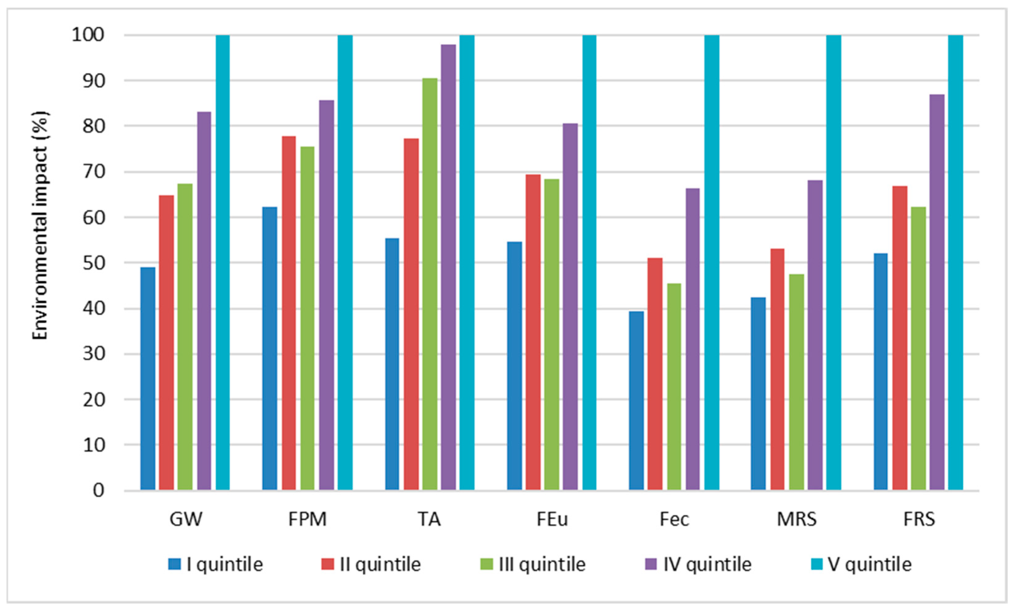
3.2. Influence of Household Income Level on Environmental Impacts

Several studies have assessed the environmental impacts of households through the LCA methodology. However, the studies have not examined household income level and how this influences environmental impacts. As Figure 2 shows, the higher the household income level (quintile 5), the higher the environmental impacts. This trend is present in all the impact categories assessed, with freshwater ecotoxicity standing out with a 61% difference between the first and fifth quintile.
In global warming, the average impact of a household in Santiago was 3.44 t CO2 eq/inh/year, with the first quintile having a value of 1.98 t CO2 eq/inh/year and the fifth quintile 4.04 t CO2 eq/inh/year. Similar values have been reported in Spanish cities, reaching 2.4 t CO2 eq/inh/year in Barcelona, 4.2 t CO2 eq/inh/year in Madrid and Seville, and 4.3 t CO2 eq/inh/year in Valencia [46]. In this category, the fifth quintile inhabitants double the environmental impacts of the first quintile, which is mainly due to fuel consumption patterns associated with transport. According to Chile’s nationally determined contributions (NDC), the carbon footprint of an average Chilean is 4.7 t CO2 eq/inh/year [48]. In this sense, the metabolism of households in Santiago accounts for 73.4% of the global warming impacts of an average Chilean inhabitant. This percentage varies from 41.9% in households in the first quintile to 85.6% in households in the fifth quintile. Similar values have been reported by Ivanova et al., (65%) [49] and Hertwich and Peters (72%) [15]. Both authors indicate that global greenhouse gas (GHG) emissions are mainly influenced by household consumption. In this sense, the carbon footprint is strongly correlated with per capita consumption expenditure [15]. That is, the higher the household consumption, the higher the GHG emissions. The latter is equivalent to the level of household income.
In Table 3, it is possible to observe the values of the impact category indicators for all the quintiles and categories evaluated. An average Santiago inhabitant generates environmental impacts of 11.3 kg PM2.5 eq/inh/year, 22.5 kg SO2 eq/inh/year, 10.3 kg P eq/inh/year, 92.9 kg 1,4-DCB eq/inh/year, 7.38 kg Cu eq/inh/year, and 710 kg oil eq/inh/year. The average values are strongly influenced by the fifth and fourth quintiles, representing 20.3% and 49.6% of households, respectively. Similar results were obtained by García-Guaiti et al. [23] for terrestrial acidification (45 kg SO2 eq/inh/year) and freshwater eutrophication (1.1 kg P eq/inh/year) for an average inhabitant of Santiago de Compostela in Spain. For the fine particulate matter formation category, the value obtained for a sample from Spain was 6 kg PM2.5 eq/inh/year [46], which is lower than the values obtained in this study. This result may be influenced by the composition of the Spanish electricity matrix where renewable energies reach values close to 40%, while coal and combined cycle represent 13.5% and 10%, respectively. In Chile, coal-based power generation represents 36.8%, which implies higher impacts on the particulate matter formation impact category.

3.3. Environmental Hotspot Analysis

Based on the contribution analysis, it was possible to identify the main household environmental hotspots. As shown in Figure 3, food consumption is the main hotspot, responsible for 33% of the environmental impacts on global warming, 69% on terrestrial acidification and 29% on freshwater eutrophication. In all three impact categories, food is the leading environmental hotspot. In the remaining categories, food accounts for between 11% and 21% of the impacts. According to Hertwich and Peters [15], nutrition is the most important consumption category, with food accounting for nearly 20% of GHG emissions. The second most important source is private transport, generating the highest impacts in the categories of freshwater ecotoxicity—with 59%; mineral resource scarcity—with 55%; fossil resource scarcity—with 35%. It is also the second most important source of global warming—with 22%. The third source of environmental importance is electricity consumption. This flow generates the highest environmental load in the category of fine particulate matter formation, accounting for 45% of the environmental impact. Other impact categories strongly influenced by electricity are freshwater eutrophication and freshwater ecotoxicity, representing the second most important environmental source with 28% and 14% of the impacts, respectively.
In Figure 3, it is possible to observe an inverse relationship between private car use and public transport, which influences the environmental impacts of each quintile. In this sense, the contribution to private transport’s environmental impact rises with household income increase, while that of public transport increases with a decrease in household income. There is no clear trend regarding the contribution to food’s environmental impacts, which is associated with the absence of trends in food consumption according to each quintile.
Within the food group, meat consumption was found to be the primary environmental source in the impact categories of global warming (50–60%), fine particulate matter formation (52–65%), terrestrial acidification (60–71%), and freshwater eutrophication (51–63%). Concurrently, processed animal products account for between 15% and 20% of the impacts in the same categories, reflecting animal foods’ contribution in all four impact categories. In the impact categories of freshwater ecotoxicity, mineral resources scarcity, and fossil resources scarcity, foods of plant origin (vegetables, processed vegetables, and fruits) are the main environmental sources, accounting for between 41% and 69% of the impacts. In this group, vegetables are the primary source, reaching up to 30% of freshwater ecotoxicity impacts, 37% in mineral resource scarcity, and 23% in fossil resource scarcity.

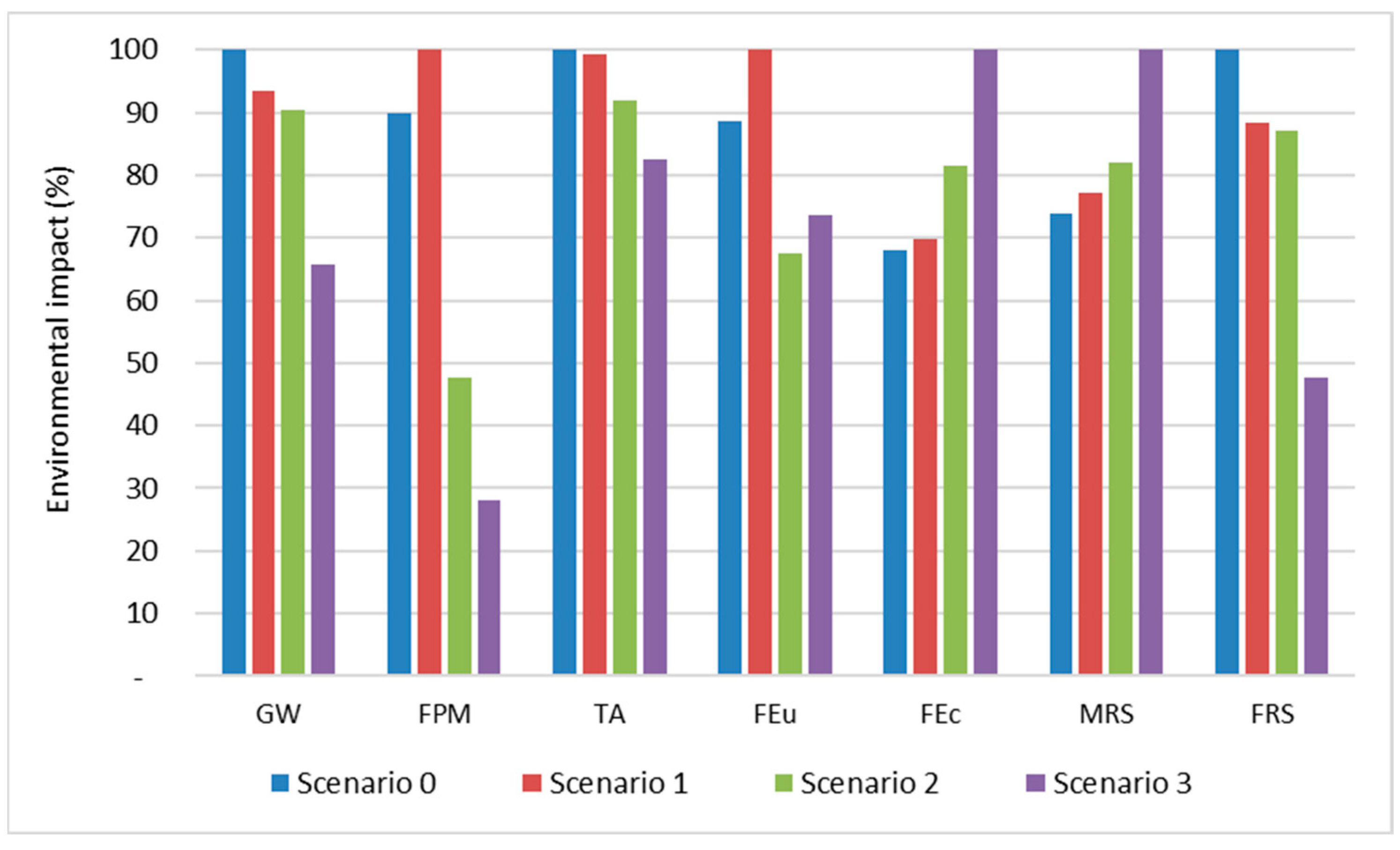
3.4. Scenarios Analysis

Based on Santiago’s modeling, the implementation of two public policies in Chile, projected to 2050, were analyzed. The first (Scenario 1), which is being applied to public transport, projects having 100% of public transport and 40% of private vehicles being electric by 2050 [43]. The second (Scenario 2), associated with energy policy, aims to have at least 70% of the total electricity generation from renewable energy by the same year [44]. Figure 1 presents the modeling of the scenarios mentioned above, the current scenario (Scenario 0), and a scenario that considers the implementation and fulfillment of both policies. It can be seen that the categories of global warming impact, freshwater acidification, and fossil resource scarcity show similar trends in all scenarios. In freshwater acidification and fossil resource, the combination of both policies in 2050 would reduce environmental impacts by 18% and 52%, respectively. In global warming, the reduction would be 34%, which would translate to a carbon footprint to decrease from 3.44 kg CO2 eq/inh/year to 2.3 kg CO2 eq/inh/year.
Furthermore, in the three impact categories mentioned above, a synergistic effect is observed when both policies are applied together. The reason for this is that, in electromobility Scenario 1, transport decreases the consumption of fossil fuels (gasoline and diesel) and increases electricity consumption. However, the change of energy generates a decrease in greenhouse gas emissions. In Scenario 2, only the consumption of fossil fuels in the energy matrix decreases, without affecting transport emissions. In Scenario 3, in addition to applying both reductions (Scenarios 1 and 2), the minimization of fossil fuels associated with electricity consumption in public and private transport is added, a factor not present in Scenarios 1 and 2. Similar results were obtained by Nissinen et al. [50] in their study on the environmental effects of combining policy instruments. They concluded that when a set of instruments is examined as a whole, as combinations of policy instruments or ‘policy packages,’ the synergies between measures can be reinforced, and hence overall effectiveness can be improved.
In the category of fine particulate matter formation, it is observed that the increase in the number of electric vehicles leads to an increase in environmental impacts. Although electric vehicles generate practically zero local emissions of particulate matter, these emissions are generated in electricity generation plants. In this sense, a vehicle loaded with electricity from a coal power plant causes by far the highest burdens in the fine particular matter formation category [51]. In Chile’s case, coal is the main contributor to the electricity matrix with 36.8%, which generates the highest environmental impacts on particulate matter formation in Scenario 2. For this reason, the increase in the electric car fleet in Santiago will have adverse effects on the fine particulate matter formation and freshwater eutrophication impact categories under the current electricity scenario in Chile. However, if electromobility of transport is implemented in conjunction with the electricity matrix’s decarbonization (Scenario 3), environmental impacts are significantly reduced. As shown in Figure 4, impacts in the fine particulate matter formation category could be reduced by up to 72%, which implies the need to move forward in conjunction with both policies.
The scenario analysis shows that the impact categories of freshwater ecotoxicity and mineral resource scarcity increase with the application of both policies, showing a negative synergistic effect on environmental impacts. In the case of freshwater ecotoxicity, the main environmental hotspot in Scenario 1 is electricity consumption. In this sense, the increase in electricity consumption due to the vehicle fleet’s change is reflected in the increase of the impact. It is important to note that the main hotspots for freshwater ecotoxicity in electricity are associated with hard coal production with about 48%, followed by photovoltaic and wind power production with 22% and 18%, respectively. These last two values are high considering that photovoltaic power currently accounts for 8.2%, and wind for 6.2%, of total energy production. As shown in Figure 1, the increase to 48.86% of photovoltaic and 27.39% of wind by 2050 will significantly increase the impacts on freshwater ecotoxicity. Thus, the increase in impacts from the change in the electricity mix, plus the increase in electricity consumption by the electric vehicle fleet, results in the negative effects on freshwater ecotoxicity in Scenario 3. In the case of the mineral resource scarcity category, a similar phenomenon occurs for freshwater ecotoxicity. In this case, future scenarios are strongly influenced by the increase in photovoltaic and wind energy and by the increase in electric cars and electric vehicle consumption. In this category, iron, nickel, aluminum, and copper are the substances that contribute to the highest environmental load. In the case of electric cars, the consumption of iron (21%), nickel (11%), copper (6%), and lithium (6%) for their production and batteries are the main environmental sources. In the 2050 electricity matrix, the consumption of iron (14%), aluminum (12%), copper (9%), and nickel (8%), mainly associated with photovoltaic panels, are primarily responsible for the impact on the scarcity of mineral resources.

4. Conclusions

From this study, it could be determined that the level of household income influences environmental impacts. In this sense, the higher the income level, the more significant the environmental impacts. Aspects associated with food, use of private vehicles, public transport, and electricity were determined to be the main environmental sources of households, and therefore, elements that should be considered in public policies applied at the urban level.
From the analysis of two long-term public policies planned in Chile, it was concluded that electromobility in public and private transport would have positive environmental effects on the categories of global warming, terrestrial acidification, and fossil fuel scarcity. However, it will generate adverse effects on fine particular matter formation, freshwater eutrophication, freshwater ecotoxicity, and mineral resource scarcity. For the policy associated with the decarbonization of the electricity grid, environmental impacts are reduced in most of the categories assessed, except for the categories of freshwater ecotoxicity and mineral resources scarcity. These two impact categories increase with each policy’s implementation, with a negative synergistic effect observed when both are met. On the contrary, achieving the goals of electromobility and increasing the share of renewable energy in the electricity mix by 2050 generates a positive synergistic effect on the household’s environmental impacts. In this sense, the application of both policies will reduce the impacts on global warming, fine particular matter formation, terrestrial acidification, and fossil fuel scarcity. Both negative and positive effects are vital for decision-making and, therefore, should be considered in consumer policies and policymaking.

Author Contributions

Formal analysis, E.M.; Funding acquisition, E.M.; Investigation, C.L.-E., E.G.-R., I.F.-A. and E.M.; Methodology, C.L.-E. and E.M.; Project administration, C.L.-E.; Software, C.L.-E. and E.M.; Supervision, E.M.; Validation, E.M.; Writing – original draft, E.M.; Writing – review & editing, E.G.-R. and I.F.-A. All authors have read and agreed to the published version of the manuscript.

Funding

This research was funded by “ANID/CONICYT FONDECYT Iniciación 11170992” of Chile.

Institutional Review Board Statement

The study was conducted according to the guidelines of the Declaration of Helsinki, and approved by Bioethics Committee of Universidad Andrés Bello, protocol code 029/2017 of 27 December 2017.

Informed Consent Statement

Informed consent was obtained from all subjects involved in the study.

Data Availability Statement

The data presented in this study are available on request from the corresponding author. The data are not publicly available due to privacy restrictions according to protocol code 029/2017

Conflicts of Interest

The authors declare no conflict of interest.

References

  1. Muñoz, E.; Navia, R. Circular economy in urban systems: How to measure the impact? Waste Manag. Res. 2021, 39, 197–198. [Google Scholar] [CrossRef]
  2. Romero-Lankao, P.; Gnatz, D.M. Conceptualizing urban water security in an urbanizing world. Curr. Opin. Environ. Sustain. 2016, 21, 45–51. [Google Scholar] [CrossRef] [Green Version]
  3. Zinatizadeh, S.; Monavari, S.M.; Azmi, A.; Sobhanardakani, S. Evaluation and prediction of sustainability of urban areas: A case study for Kermanshah city, Iran. Cities 2017, 66, 1–9. [Google Scholar] [CrossRef]
  4. Nations, U. World Urbanization Prospects: The 2018 Revision; United Nations: New York, NY, USA, 2019; Volume 12. [Google Scholar]
  5. Hertwich, E.G. Life cycle approaches to sustainable consumption: A critical review. Environ. Sci. Technol. 2005, 39, 4673–4684. [Google Scholar] [CrossRef] [PubMed]
  6. United Nations. The System of National Accounts 2018; United Nations: New York, NY, USA, 2009. [Google Scholar]
  7. Di Donato, M.; Lomas, P.L.; Carpintero, Ó. Metabolism and environmental impacts of household consumption: A review on the assessment, methodology, and drivers. J. Ind. Ecol. 2015, 19, 904–916. [Google Scholar] [CrossRef]
  8. Tukker, A. Identifying priorities for environmental product policy. J. Ind. Ecol. 2006, 10, 1–4. [Google Scholar] [CrossRef]
  9. Caeiro, S.; Ramos, T.B.; Huisingh, D. Procedures and criteria to develop and evaluate household sustainable consumption indicators. J. Clean. Prod. 2012, 27, 72–91. [Google Scholar] [CrossRef]
  10. Froemelt, A.; Dürrenmatt, D.J.; Hellweg, S. Using Data Mining to Assess Environmental Impacts of Household Consumption Behaviors. Environ. Sci. Technol. 2018, 52, 8467–8478. [Google Scholar] [CrossRef]
  11. Matuštík, J.; Kočí, V. Environmental impact of personal consumption from life cycle perspective—A Czech Republic case study. Sci. Total Environ. 2019, 646, 177–186. [Google Scholar] [CrossRef]
  12. Newton, P.; Meyer, D. The determinants of urban resource consumption. Environ. Behav. 2012, 44, 107–135. [Google Scholar] [CrossRef]
  13. Kalbar, P.P.; Birkved, M.; Hauschild, M.; Kabins, S.; Nygaard, S.E. Environmental impact of urban consumption patterns: Drivers and focus points. Resour. Conserv. Recycl. 2018, 137, 260–269. [Google Scholar] [CrossRef]
  14. Castellani, V.; Beylot, A.; Sala, S. Environmental impacts of household consumption in Europe: Comparing process-based LCA and environmentally extended input-output analysis. J. Clean. Prod. 2019, 240, 117966. [Google Scholar] [CrossRef]
  15. Hertwich, E.G.; Peters, G.P. Carbon footprint of nations: A global, trade-linked analysis. Environ. Sci. Technol. 2009, 43, 6414–6420. [Google Scholar] [CrossRef] [Green Version]
  16. Davis, S.J.; Caldeira, K. Consumption-based accounting of CO 2 emissions. Proc. Natl. Acad. Sci. USA 2010, 107, 5687–5692. [Google Scholar] [CrossRef] [Green Version]
  17. Hoekstra, A.Y.; Mekonnen, M.M. The water footprint of humanity. Proc. Natl. Acad. Sci. USA 2012, 109, 3232–3237. [Google Scholar] [CrossRef] [PubMed] [Green Version]
  18. Bruckner, M.; Fischer, G.; Tramberend, S.; Giljum, S. Measuring telecouplings in the global land system: A review and comparative evaluation of land footprint accounting methods. Ecol. Econ. 2015, 114, 11–21. [Google Scholar] [CrossRef] [Green Version]
  19. Lausselet, C.; Ellingsen, L.A.W.; Strømman, A.H.; Brattebø, H. A life-cycle assessment model for zero emission neighborhoods. J. Ind. Ecol. 2020, 24, 500–516. [Google Scholar] [CrossRef]
  20. Kim, D.; Parajuli, R.; Thoma, G.J. Life cycle assessment of dietary patterns in the United States: A full food supply chain perspective. Sustainability 2020, 12, 1586. [Google Scholar] [CrossRef] [Green Version]
  21. Ng, K.S.; To, L.S. A systems thinking approach to stimulating and enhancing resource efficiency and circularity in households. J. Clean. Prod. 2020, 275, 123038. [Google Scholar] [CrossRef]
  22. Matuštík, J.; Kočí, V. A comparative life cycle assessment of electronic retail of household products. Sustainability 2020, 12, 4604. [Google Scholar] [CrossRef]
  23. García-Guaiti, F.; González-García, S.; Villanueva-Rey, P.; Moreira, M.T.; Feijoo, G. Integrating Urban Metabolism, Material Flow Analysis and Life Cycle Assessment in the environmental evaluation of Santiago de Compostela. Sustain. Cities Soc. 2018, 40, 569–580. [Google Scholar] [CrossRef]
  24. Sala, S.; Castellani, V. The consumer footprint: Monitoring sustainable development goal 12 with process-based life cycle assessment. J. Clean. Prod. 2019, 240, 118050. [Google Scholar] [CrossRef] [PubMed]
  25. Azimi, A.N.; Dente, S.M.R.; Hashimoto, S. Social life-cycle assessment of householdwaste management system in Kabul city. Sustainability 2020, 12, 3217. [Google Scholar] [CrossRef] [Green Version]
  26. Tran, H.P.; Schaubroeck, T.; Nguyen, D.Q.; Ha, V.H.; Huynh, T.H.; Dewulf, J. Material flow analysis for management of waste TVs from households in urban areas of Vietnam. Resour. Conserv. Recycl. 2018, 139, 78–89. [Google Scholar] [CrossRef]
  27. Leray, L.; Sahakian, M.; Erkman, S. Understanding household food metabolism: Relating micro-level material flow analysis to consumption practices. J. Clean. Prod. 2016, 125, 44–55. [Google Scholar] [CrossRef]
  28. ISO. Environmental Management—Life Cycle Assessment—Principles and Framework; ISO: Geneva, Switzerland, 2006. [Google Scholar]
  29. ISO. Environmental Management—Life Cycle Assessment—Requirements and Guidelines; ISO: Geneva, Switzerland, 2006. [Google Scholar]
  30. SII Cartografía Digital SII Mapas. Available online: https://www4.sii.cl/mapasui/internet/#/contenido/index.html (accessed on 14 August 2018).
  31. INE. Informe de Principales Resultados VIII Encuesta de Presupuestos Familiares (EPF); INE: Santiago, Chile, 2018. [Google Scholar]
  32. Muñoz, E.; Curaqueo, G.; Cea, M.; Vera, L.; Navia, R. Environmental hotspots in the life cycle of a biochar-soil system. J. Clean. Prod. 2017, 158, 1–7. [Google Scholar] [CrossRef]
  33. CNE. Anuario Estadístico de Energía 2019; CNE: Santiago, Chile, 2020. [Google Scholar]
  34. Ministerio de Transportes y Telecomunicaciones, Informe de Evaluación Externa al Sistema de Transporte Público Remunerado de Pasajeros de la Provincia de Santiago y de las Comunas de San Bernardo y Puente Alto. Available online: http://biblioteca.digital.gob.cl/handle/123456789/972 (accessed on 1 January 2021).
  35. DTP. Mejoramiento y Actualización del Modelo de Asignación de viajes del Sistema Transantiago; DTP: Santiago, Chile, 2018. [Google Scholar]
  36. Abello-Passteni, V.; Muñoz Alvear, E.; Lira, S.; Garrido-Ramírez, E. Evaluación de Eco-Eficiencia de Tecnologías de Tratamiento de Aguas Residuales Domésticas en Chile. Tecnología y Ciencias del Agua 2020, 11, 190–228. [Google Scholar] [CrossRef] [Green Version]
  37. Gaete-Morales, C.; Gallego-Schmid, A.; Stamford, L.; Azapagic, A. Assessing the environmental sustainability of electricity generation in Chile. Sci. Total Environ. 2018, 636, 1155–1170. [Google Scholar] [CrossRef] [PubMed] [Green Version]
  38. Montalba, R.; Vieli, L.; Spirito, F.; Muñoz, E. Environmental and productive performance of different blueberry (Vaccinium corymbosum L.) production regimes: Conventional, organic, and agroecological. Sci. Hortic. (Amsterdam) 2019, 256, 108592. [Google Scholar] [CrossRef]
  39. Muñoz, E.; Navia, R.; Zaror, C.; Alfaro, M. Ammonia emissions from livestock production in chile: An inventory and uncertainty analysis. J. Soil Sci. Plant Nutr. 2016, 16, 60–75. [Google Scholar] [CrossRef] [Green Version]
  40. Herrera, J.; Muñoz, E.; Montalba, R. Evaluation of two production methods of Chilean wheat by life cycle assessment (LCA). IDESIA 2012, 30, 101–110. [Google Scholar] [CrossRef] [Green Version]
  41. Bezama, A.; Douglas, C.; Méndez, J.; Szarka, N.; Muñoz, E.; Navia, R.; Schock, S.; Konrad, O.; Ulloa, C. Life cycle comparison of waste-to-energy alternatives for municipal waste treatment in Chilean Patagonia. Waste Manag. Res. 2013, 31, 67–74. [Google Scholar] [CrossRef]
  42. Gajardo, S. Pobreza y distribución del ingreso en la Región Metropolitana de Santiago: Resultados Encuesta CASEN 2015. Available online: https://www.desarrollosocialyfamilia.gob.cl/storage/docs/DOCUMENTO_POBREZA_Y_DISTR_ING_RMS_CASEN_2017.pdf (accessed on 1 January 2021).
  43. Ministerio de Energía—Gobierno de Chile. Estrategia Nacional de Electromovilidad; Santiago, Chile. 2017. Available online: https://energia.gob.cl/sites/default/files/estrategia_electromovilidad-8dic-web.pdf (accessed on 1 January 2021).
  44. Ministerio de Energía—Gobierno de Chile. Energía 2050—Política Energética de Chile; Santiago, Chile. 2015. Available online: https://observatoriop10.cepal.org/es/instrumentos/politica-energetica-chile-energia-2050 (accessed on 1 January 2021).
  45. Superintendencia de Servicios Sanitarios (SISS)—Gobierno de Chile. Informe de Gestión del Sector Sanitario; Santiago, Chile. 2019. Available online: https://www.coursehero.com/file/75668465/Informe-de-gestion-sector-sanitario-SISS-2019pdf/ (accessed on 1 January 2021).
  46. Gonzalez-Garcia, S.; Manteiga, R.; Moreira, M.T.; Feijoo, G. Assessing the sustainability of Spanish cities considering environmental and socio-economic indicators. J. Clean. Prod. 2018, 178, 599–610. [Google Scholar] [CrossRef]
  47. SUBDERE—Gobierno de Chile. In Diagnostico de la Situación por Comuna y por Región en Materia de Residuos Sólidos Domiciliarios y Asimilables; Santiago, Chile; 2018. Available online: http://www.subdere.gov.cl/sites/default/files/4.1_diagnostico_introduccion_agosto_2018.pdf (accessed on 1 January 2021).
  48. Gobierno de Chile. Contribución Determinada a Nivel Nacional (NDC) de Chile; Santiago, Chile. 2020. Available online: https://mma.gob.cl/wp-content/uploads/2019/10/Propuesta_actualizacion_NDC_Chile_2019.pdf (accessed on 1 January 2021).
  49. Ivanova, D.; Stadler, K.; Steen-Olsen, K.; Wood, R.; Vita, G.; Tukker, A.; Hertwich, E.G. Environmental Impact Assessment of Household Consumption. J. Ind. Ecol. 2016, 20, 526–536. [Google Scholar] [CrossRef]
  50. Nissinen, A.; Heiskanen, E.; Perrels, A.; Berghäll, E.; Liesimaa, V.; Mattinen, M.K. Combinations of policy instruments to decrease the climate impacts of housing, passenger transport and food in Finland. J. Clean. Prod. 2015, 107, 455–466. [Google Scholar] [CrossRef]
  51. Bauer, C.; Hofer, J.; Althaus, H.J.; Del Duce, A.; Simons, A. The environmental performance of current and future passenger vehicles: Life Cycle Assessment based on a novel scenario analysis framework. Appl. Energy 2015, 157, 871–883. [Google Scholar] [CrossRef]
Figure 1. Product system used for the life cycle analysis of a household. T: transport, D: distribution.
Sustainability 13 02525 g001
Figure 2. Comparison of environmental impacts of households at different income levels. GW: Global warming, FPM: Fine particulate matter formation, TA: Terrestrial acidification, FEu: Freshwater eutrophication, FEc: Freshwater ecotoxicity, MRS: Mineral resource scarcity, FRS: Fossil resource scarcity.
Sustainability 13 02525 g002
Figure 3. Household environmental contribution analysis by income level (quintile).
Sustainability 13 02525 g003
Figure 4. Comparative analysis of household scenarios in Santiago. Scenario 0: current situation; Scenario 1: 100% electric public transport, 40% electric private transport, and electricity grid 2019; Scenario 2: electricity matrix 2050; Scenario 3: Public transport 100% electric, private transport 40%, and electricity grid 2050. GW: Global warming, FPM: Fine particulate matter formation, TA: Terrestrial acidification, FEu: Freshwater eutrophication, FEc: Freshwater ecotoxicity, MRS: Mineral resource scarcity, FRS: Fossil resource scarcity.
Sustainability 13 02525 g004
Table 1. Distribution of Santiago inhabitants in quintiles according to household per capita income level (adapted from [42]).
QuintileFrom (USD)To (USD)Households Share (%)
I01205.8
II12021010.1
III21031514.2
IV31556020.3
V560--49.6
Table 2. Summary of life cycle inventory data of the foreground associated with the functional unit.
SubsystemUnitHousehold Income Quintile
IIIIIIIVV
Waterm3/inh/year55.468.966.083.490.5
Fruitskg/inh/year28.452.157.952.854.1
Vegetableskg/inh/year86.0140.1142.0140.4119.4
Legumeskg/inh/year8.317.018.219.214.2
Processed productskg/inh/year100.4140.7139.8122.4101.2
Dairy productskg/inh/year21.940.640.941.950.6
Porkkg/inh/year2.16.610.16.94.6
Chickenkg/inh/year9.613.814.820.115.8
Beefkg/inh/year7.210.312.815.815.7
Municipal solid wastekg/inh/year153.7295.7218.8369.9637.2
ElectricitykWh/inh/year569.7778.0753.2861.71204.5
Liquefied petroleum gaskWh/inh/year750011,38910,27816,6677222
KerosenekWh/inh/year277.8527.8305.6611.1555.6
Natural gaskWh/inh/year55.6277.81944.41388.93333.3
GasolinekWh/inh/year61116389472210,55621,389
Diesel fuelkWh/inh/year01944.42222.23333.35277.8
Wastewaterm3/inh/year44.355.152.866.772.4
Table 3. Household environmental impact assessment by income level (quintile).
Impact CategoryUnitHousehold Income Quintile
IIIIIIIVV
Global warmingkg CO2 eq19802616272633634038
Fine particulate matter formationkg PM2.5 eq7.99.99.610.912.7
Terrestrial acidificationkg SO2 eq13.318.621.823.624.1
Freshwater eutrophicationkg P eq0.650.830.820.971.20
Freshwater ecotoxicitykg 1,4-DCB47.561.754.880.0120.7
Mineral resource scarcitykg Cu eq4.05.04.56.49.5
Fossil resource scarcitykg oil eq431553515719828
Publisher’s Note: MDPI stays neutral with regard to jurisdictional claims in published maps and institutional affiliations.

