Application of Exact and Multi-Heuristic Approaches to a Sustainable Closed Loop Supply Chain Network Design

Abstract

Closed-loop supply chains (CLSC) are gaining popularity due to their efficiency in addressing economic, environmental, and social concerns. An important point to ponder in the distribution of CLSC is that imperfect refrigeration and bad road conditions may result in product non-conformance during the transit and thus such products are to be returned to the supply node. This may hinder the level of customer satisfaction. This paper presents a sustainable closed-loop supply chain framework coupled with cross-docking subject to product non-conformance. A cost model is proposed to investigate the economic and environmental aspects of such systems. The transportation cost is analyzed in terms of total carbon emissions. A set of metaheuristics are administered to solve the model and a novel lower bound is proposed to relax the complexity of the proposed model. The results of different size problems are compared with the branch and bound approach and the proposed lower bound. The results indicate that the proposed research framework, mathematical model, and heuristic schemes can aid the decision-makers in a closed-loop supply chain context.

1. Introduction

Modern manufacturing systems are faced with enormous challenges in a resource constrained environment. These challenges are in the form of supply chain issues, business growth, and responsiveness towards customers. These issues can be addressed through an efficient design of production systems, cost-efficient manufacturing, improved quality of products, and green logistics management. During the last few years, green logistics have attained prime attention and have become an indispensable part of the overall supply chain because it provides a mechanism for end-to-end transportation with social and ecological benefits, i.e., sustainable approaches. The literature shows that the cost related to logistics contributes towards the total sales value by more than 35%.

The performance of organizations involved in closed loop networks and green practices can be affected and fostered by the culture at the heart of an organization and the leadership role offered by the top management. Suryaningtyas et al. [1] argued that a strategic management focus, resilience within an organization and the leadership role play an active role in boosting the overall performance in the wake of disruptive challenges. Further, as CLSC networks are designed to improve sustainable developments, several factors can be identified at the level of an organization that can help the management in achieving the sustainability landmarks. Several management level decisions were examined by Drobyazko et al. [2] such as, financial, psychological, social, and economic factors that can offer an enabling environment to implement sustainable practices at an organization.

In modern times, the notion of sustainability encompasses approaches adopted in manufacturing, transportation, and vehicle distribution. The emissions during manufacturing are related to and can be restricted to the boundary of the manufacturing system; however, more sustainable approaches need to be adopted to cater to the emissions during transportation and vehicle distribution as they are directly related to the well-being of society. In this regard, cost models can be proposed to calculate the impact of emissions caused by vehicles during transportation.

Presently, greenhouse gas emissions (GHG), especially carbon dioxide emissions, have attracted growing concern worldwide. In this perspective, regulatory authorities are trying to enforce strict legislations for a low-carbon economy with clean products [3]. Considering this, closed loop supply chain and dispatching strategies can be tailored to optimize and minimize fuel consumption which in return reduces the carbon emissions. Some excellent research studies have been reported which demonstrated the statistics and relationship among reducing travel mileage, fuel consumption, and saving in GHG emissions [4]. From the studies [5,6]), it is evident that carbon emissions are linearly proportional to fuel consumption. This performance parameter greatly depends on the vehicle condition, type, gross weight, and dispatch time (travel speed). A salient feature of logistics and inventory design is cross-docking which has proved to be effective in controlling the distribution costs and maintaining an utmost level of customer satisfaction [7]. An important problem from the sustainability viewpoint is closed loop supply chain with cross-docking. It represents the most discussed class of combinatorial problems.

Though different contributions have been offered towards the analysis of such problems, the analysis based on defective products and product return by using a lower bound is missing in the concerned literature. The novelty of this study can be defined in terms of framework, methodology, and the analysis of emissions. In the framework, a closed loop supply chain (CLSC) network is designed keeping in view an imperfect product delivery. Traditionally, CLSC networks have been studied where products are delivered in a perfect state of quality. However, the quality-loss of product during transit may occur due to imperfect refrigeration, road conditions, traffic bottlenecks and different quality conditions of multiple products. This quality-loss may result in defective products that are to be returned. In terms of methodology, an initial heuristic is embedded with the simulated annealing to enhance its computational efficiency. The benchmark experiments inform that the initial heuristic embedded with simulated annealing performs well. Further, a novel lower-bound is proposed to relax the computational complexity of the model. It is defined in terms of cost. Lastly, as emissions are central in a sustainable supply chain framework, a comparison between emissions in terms of distance and DEFRA based results is presented. The Department for Environment, Food and Rural Affairs (DEFRA) takes the relative CO₂ per kilometer performance of the European Environment Agency (EEA) CO₂ monitoring database source as the payload capacity information.

This study considers a closed loop supply chain with cross-docking (CLSCCD). A cost-minimization model is proposed to assess the effectiveness of CLSCCD. The presented study considers a defect-based system where forward and returned goods are analyzed by considering the non-conformance of products, penalty, and product return. The cost components used in the model are related to production, transportation, handling, penalty, and the cost of product return. The reduced dispatching cost has been analyzed in terms of fuel savings and reduction in carbon dioxide for a greener environment. A mixed integer non-linear programming (MINLP) model is presented, and multi-heuristic approaches are used for model implementation. Moreover, the presented study is unique in the aspect that it offers a novel lower bound approach for CLSCCD.

The remaining study is organized as follows. Section 2 provides literature related to the CLSCCD, Section 3 outlines the problem description, Section 4 contains the detailed model, Section 5 provides the heuristic approaches, lower bound, parameter tuning, and benchmark experiments. Section 6 provides the results and Section 7 offers the conclusion and future research avenues related to CLSCCD.

2. Literature Review

CLSC frameworks have been thoroughly analyzed in the relevant literature and different models have been proposed to advance this field of research. This section presents the review of literature according to the focus of different objective functions, solution approaches adapted to address the problems, environmental concerns in CLSC, the emergence of green practices in CLSC design and a review of solution approaches.

2.1. CLSC Network, Environmental Concerns, and Green Practices

Several authors have identified key factors that affects the performance of CLSC networks. Choi et al. [8] studied the delivery schedule by employing an Ant Colony Optimization algorithm and predicted a comprehensive strategy to reduce carbon emissions. Likewise, Suzuki [4] proposed that sustainable scheduling with an expert decision-making system for speed and load can significantly reduce the carbon emissions. Qian and Eglese [9] also highlighted that dispatching time (speed) depends on several factors and a road network. They developed a column generation-based TS algorithm and tested real traffic data. Miao et al. [10] developed an adaptive real-time optimization strategy and concluded that vehicle dynamic parameters have a great impact on fuel economy.

Elhedhli and Merrick [11] studied the supply chain problem considering the environmental costs resulting from CO₂ emissions alongside fixed and variable factors. Pishvaee et al. [12] presented a mixed-integer programming (MIP) model for developing a reverse logistics network. They solved the non-polynomial hard (NP-hard) problem by employing a Simulated Annealing (SA) algorithm with neighborhood structures. Kannan et al. [13] studied the model proposed by Pishvaee et al. [12] by incorporating the environmental impacts due to carbon emissions. Faccio et al. [14] proposed a linear programming model to minimize the total cost in a supply chain. Their work evaluated the economic sustainability of the model by performing parametric analysis. Mota et al. [15] argued that while dealing with the sustainable supply chain problems, economic, environmental, and social dimensions are not considered realistically. Fonseca et al. [16] proposed a bi-objective model considering the total costs and environmental impacts with two-phase stochastic programming.

One of the central decisions in a CLSC network is to identify the relevant transportation routes which can help optimize the overall performance of the network. A transportation problem in CLSC can be modeled according to truck capacity, routes, and docks. The truck capacity involves decisions regarding the number and size of trucks to maximize the responsiveness of the supply chain. Routing considers different available options for the product delivery. Docking is the deployment of inter-modal facilities for product storage and consolidation purposes. A decision is made whether a cross dock is needed between the supply and demand node; depending on the capacity, number, and location of cross-docks to minimize the transportation time, and product handling costs. For instance, Vate and Zhang [17] studied a transportation network to optimize the delivery mechanism. Their work investigated the quantity and placement of cross-docks for an efficient transportation network. Noteworthy contributions can be found in the beverage and food industry where different types of routing, such as routing with time window, pickup and deployment, and distance-based routing have been used [18].

An earlier contribution towards the relevant problem type was offered by [19]. It used a mathematical model for minimizing the transportation and operation costs. Musa et al. [20] studied a vehicle routing problem where direct delivery to the customer as well as delivery through cross-docking were analyzed using MILP and ant colony optimization (ACO). In Khan [21], MILP model was proposed to analyze a multi-node transportation network. The model proved to be robust as significant cost reduction was demonstrated.

The CLSC networks are important from the viewpoint of a sustainable distribution design. They have attracted scholarly discussions in the areas of supply chain and cross-docking to address the situations where several destination points are visited by a group of vehicles for demand satisfaction. The demands are satisfied in accordance with the objective functions (cost, time, and responsiveness, etc.) and end-of-life products are retrieved back to the origin. Govindan et al. [22] highlighted the importance of closed-loop supply chain network design due to the emergence of environmental concerns and social issues. It is evident that besides focusing on the production of green products, hazardous emissions of supply chain activities during the transportation operations in both forward and reverse logistics needs to be addressed for enhanced green closed-loop supply chain management (e.g., Rahmani and Yavari [23]). In this perspective, numerous studies have been reported grounding on the mathematical modeling and heuristic optimization of CLSC problems with social-economic objectives (e.g., Kaya and Urek [24]). In this study, the proposed model considers diverse objectives that manipulate the design of closed-loop integration in forwarding/reverse supply.

In continuation to the preceding discussion, the term green closed-loop supply chain has gained prime attention by many researchers due to its undeniable advantages. For example, Talaei et al. [25] worked on a Fuzzy Mixed Integer Programming (FIMP) model for a green closed-loop supply chain and proposed important findings. Likewise, Ramezani et al. [26] developed a stochastic multi-objective model for designing a forward/reverse supply chain network in an uncertain environment of demand and the return rate. Sabulan et al. [27] developed a two-objective model for a closed-loop supply chain by applying Taguchi design experiments and evaluated the effect of different functions on the overall cost. Some researchers have sought the importance of supply chain integration in other domains, like construction [28], tire industry, auto parts manufacturing by including different dimensions of sustainability [29]. Mostafa et al. [30] developed a sustainable closed-loop supply chain network design with discount supposition. They applied a mixed-integer nonlinear programming model to formulate a multi-objective sustainable closed-loop supply chain network design in the transportation costs for a real industrial example in the glass industry.

2.2. Solution Approaches Used in CLSC Network Design

The design of CLSC networks considers multiple decisions that enhance its computational needs and makes it a complex class of problems. It involves multiple transportation options, dispatching facilities, customer locations, and cross-docks which make it computationally hard [31]. To solve such complex problems, different meta-heuristic approaches can be found in the literature [32]. Song and Chen [33] used an NP-hard approach for minimizing the total time in a two-stage based cross dock. Production planning and scheduling were performed by presenting an analogy between cross-docking and a manufacturing setup. In another study, Jayaraman and Ross [34] provided a simulated annealing approach to identify the placement of cross-docks and distribution of demand. In another study, a detailed cross-dock optimization model was proposed which incorporated both cross-dock placement and the identification of improved network paths [35].

Gholizadeh and Fazlollahtabar [36] studied a robust optimization model of a green closed loop supply chain in an uncertain environment. The authors used a modified form of genetic algorithm (GA) that comprised of seven different parts. The modified version of GA was compared with an exact solution approach and the classical GA. The results suggested that the former approach has good convergence ability. Gaur et al. [37] studied the effect of disruption on the performance of the supply chain. A non-linear model was implemented on an automotive case study by using different scenarios. An outer approximation approach was used for implementing the model. Turki et al. [38] studied four different decision aspects in a CLSC network, i.e., the capacity of manufacturing stocks, purchasing warehouse and vehicle and optimal level of returned products. A genetic algorithm was used for implementing the model and for analysing various aspects of decision making.

Cheraghalipour et al. [39] studied the CLSC network for citrus distribution and proposed a model for minimization of cost and enhancing customer responsiveness. A multi-objective Kushtal algorithm was proposed which proved effective when compared to other evolutionary solution approaches. Yavari and Geraeli [40] optimized the objectives of cost and environmental pollutants in a green CLSC network. A heuristic called YAG was implemented to solve the practical size problem instances. The results indicated that YAG had a good solution accuracy and it found solutions for more than one-third of the problem instances. Rad and Nahavandi [41] studied a multi-objective, multi-echelon, and multi-period CLSC model for multiple products. The model was solved by using an exact solution approach in CPLEX. Taleizadeh et al. [42] studied the pricing, quality, and effort in two types of decentralized CLSC networks. A game theoretic approach was used for analysing various aspects of the network design.

To summarize, different exact and evolutionary (meta-heuristic) approaches have been used to solve the CLSC problems. Compared to the earlier approaches, the novelty of present solution approach is two-fold. Firstly, a combination of Tabu search and simulated annealing (SA) approaches are used in this study. SA is used in a hybrid form by embedding an initial heuristic with it. The initial heuristic offers the current solution to obtain a derived solution. Secondly, to reduce the complexity of the presented model, a novel lower-bound (LB) is defined in terms of cost by splitting the model into forward and reverse supply chains.

Table 1. Summary of CLSC Literature.

Authors	Solution Approaches						Objectives
	NSGA-II	MILP	ACO	MOPSO	Simulation	AMOSA	Cost Minimization	Truck Selection and Uncertain Demand Environment	Capacitated Problem Analysis	Risk Management	Strategic Transport Mechanism	Routing	Quantity Discount
Ozdemir et al. [43]	×	✓	×	×	×	×	×	×	✓	×	×	×	×
Khan [21]	×	✓	×	×	×	×	✓	×	×	×	×	×	×
Hong et al. [44]	×	×	✓	×	×	×	✓	×	×	×	×	×	×
Babaveisi et al. [45]	✓	×	×	✓	×	×	✓	×	×	×	×	×	×
Zhang et al. [46]	✓	×	×	×	×	×	×	✓	×	×	×	×	×
Behzadi et al. [47]	×	✓	×	×	×	×	×	×	×	✓	×	×	×
Bhattacharya et al. [48]	×	✓	×	×	×	×	×	×	×	×	✓	×	×
Cheng et al. [49]	✓	×	×	×	×	×	×	×	✓	×	×	×	×
De Jong et al. [50]	×	×	×	×	✓	×	×	×	×	×	✓	×	×
Yildizbaşi et al. [51]	×	✓	×	×	×	×	×	×	✓	×	×	×	×
Ekren et al. [52]	×	×	×	×	✓	×	×	×	✓	×	×	×	×
Fakhrzad et al. [53]	✓	×	×	×	×	×	✓	×	×	×	×	×	×
Kawamura et al. [54]	×	✓	×	×	×	×	✓	×	×	×	×	×	×
Lu et al. [52,55]	×	✓	×	×	×	×	×	×	✓	×	×	×	×
Mejjaouli et al. [56]	×	✓	×	×	×	×	✓	×	×	×	×	✓	×
Panicker et al. [57]	×	×	✓	×	×	×	×	×	✓	×	×	✓	×
Rais et al. [58]	×	✓	×	×	×	×	×	×	×	×	✓	✓	×
Rad et al. [41]	×	✓	×	×	×	×	×	×	×	×	✓	×	✓
Singh et al. [59]	×	✓	×	×	×	×	×	×	×	×	×	✓	×
Liu et al. [60]	✓	×	×	×	×	✓	✓	×	×	×	×	✓	×
Validi et al. [61]	✓	✓	×	×	×	×	×	×	×	×	×	✓	×
Zheng et al. [62]	✓	✓	×	×	×	×	×	✓	×	✓	×	×	×

presents the summary of relevant literature according to the choice of objective functions and the application of different solution approaches. It can be observed that different meta-heuristics have been applied to solve the relevant problems; however, there is a dearth of application of multiple and hybrid meta-heuristics. This study uses multiple heuristics in the form of ant colony optimization (ACO) and Tabu search. The ACO is used in a hybrid form by embedding an initial heuristic with it to improve its computational efficiency. In terms of objective functions, the cost is the most opted choice of the objective function. The current study considers novel cost factors due to emissions and product failure. To summarize, there are some imperative differences and contributions in the proposed model from the published studies, for instance, the mathematical model explores closed-loop configuration for determining optimum cost supported by the meta-heuristic algorithm and lower bound approaches.

This paper fills the literature gap by using meta-heuristic approaches to solve a closed-loop Supply Chain Network Design (SCND) considering lower bound and some other novel aspects in this research domain. It addresses a sustainable closed-loop supply chain network along with cross-docking operations. The proposed robust model provides a comprehensive guideline to assist stakeholders in the closed-loop supply chain to make integrated decisions regarding the forward and reverse flows based on realistic assumptions. Although numerous contributions have been offered towards the analysis of cost in a closed loop supply chain, the novelty of current study rests in the following points:

• The analysis of non-conformance of products and product return routes has been considered. A mathematical model is developed by integrating different cost components involved in the supply chain of a cross-docking problem. The optimized routing cost has been discussed and analyzed from the perspective of fuel-saving which in turn reduces GHG emissions. Further, a comparison between emissions in terms of distance and DEFRA based results is presented.
• A two-method based approach is presented to solve the simple and complex problems related to CLSCCD. The simple problem instances are solved using the branch-and-bound approach while the complex problem instances are solved using two heuristics namely, Tabu Search and Simulated Annealing (SA). An initial heuristic is embedded with SA to enhance its computational efficiency. The solutions of different approaches are examined using benchmark data.
• A lower bound approach has been proposed. The meta-heuristics are evaluated against the branch-and-bound method (CPLEX) and the proposed lower bound (LB) approach using small and large problem instances, respectively. A comparison is carried out between the current findings and the established results in literature.
• A sensitivity analysis between various aspects of a CLSC in the form of vehicle capacity, conformance of products, number of trucks and customer satisfaction is presented which will help the managers in considering real-time decisions.

3. Problem Description

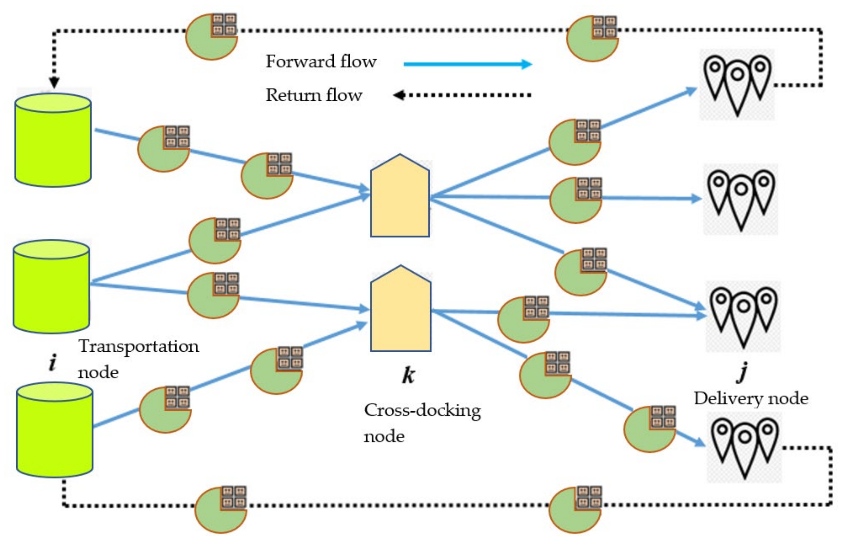
The schematic description of the CLSC problem with cross-docking is explained with the help of Figure 1. It considers the transportation of goods from node i (transportation node) to node j (delivery node) through node k (cross-dock node) by using distribution trucks. Due to perishability and breakage, some of the products are no longer required by customers and the rejected lot is sent back to the origin (node i). Two flows, i.e., forward and return flows are considered. The forward flow is a two-echelon network in which goods are initially sent to the cross-docking point (k). The items are sorted/consolidated at this point and are shipped to the delivery node (j). The return flow bypasses the cross-docking point, and it ships the non-optimal goods back to node i (this flow is described by the dotted line).

The facilities have a maximum capacity limit which is to be respected. Also, these locations are placed at a defined distance which is used in the calculation of transportation cost. A fleet of available trucks with loading capacity (LC) is used for delivering the products according to the level of demand. The goal is to accomplish product delivery by minimizing travelling, holding, penalty, return, and manufacturing costs.

4. Mathematical Model

$$\mathit{minimize} \mathit{TC}$$

(1)

$$TC=TR+DC+RC+HC$$

(2)

$$TR={\displaystyle \sum }_{k\in K}{\displaystyle \sum }_{i\in I}N{X}_{ik}\times Q{P}_{ik}\times cm+{\displaystyle \sum }_{k\in K}{\displaystyle \sum }_{i\in I}N{X}_{ik}\times N{W}_{ik}\times d{x}_{ik}+cd$$

(3)

$$DC={\displaystyle \sum }_{k\in K}{\displaystyle \sum }_{j\in J}M{X}_{kj}\times F{P}_{kj}\times cm+{\displaystyle \sum }_{k\in K}{\displaystyle \sum }_{j\in J}M{X}_{kj}\times M{W}_{kj}\times d{y}_{kj}+cd$$

(4)

$$RC={\displaystyle \sum }_{i\in I}{\displaystyle \sum }_{j\in J}R{X}_{ji}\times P{R}_{ji}\times \left(cm+cp+cr\right)+{\displaystyle \sum }_{i\in I}{\displaystyle \sum }_{j\in J}R{X}_{ji}\times T{W}_{ji}\times d{z}_{ji}+cd$$

(5)

$$HC=ch({\displaystyle \sum }_{k\in K}{\displaystyle \sum }_{i\in I}N{X}_{ik}\times Q{P}_{ik}-{\displaystyle \sum }_{k\in K}{\displaystyle \sum }_{j\in J}M{X}_{kj}\times F{P}_{kj})$$

(6)

$${\displaystyle \sum }_{k\in K}{\displaystyle \sum }_{i\in I}N{W}_{ik}\times LC\ge {\displaystyle \sum }_{k\in K}{\displaystyle \sum }_{i\in I}Q{P}_{ik}$$

(7)

$${\displaystyle \sum }_{k\in K}{\displaystyle \sum }_{j\in J}M{W}_{kj}\times LC\ge {\displaystyle \sum }_{k\in K}{\displaystyle \sum }_{j\in J}F{P}_{kj}$$

(8)

$${\displaystyle \sum }_{i\in I}{\displaystyle \sum }_{j\in J}T{W}_{ji}\times LC\ge {\displaystyle \sum }_{i\in I}{\displaystyle \sum }_{j\in J}P{R}_{ji}$$

(9)

$${\displaystyle \sum }_{i\in I}{\displaystyle \sum }_{k\in K}N{W}_{ik}>{\displaystyle \sum }_{k\in K}{\displaystyle \sum }_{j\in J}M{W}_{kj}$$

(10)

$${\displaystyle \sum }_{i\in I}{\displaystyle \sum }_{k\in K}Q{P}_{ik}\le mx\hspace{1em}\forall i\in I$$

(11)

$${\displaystyle \sum }_{i\in I}{\displaystyle \sum }_{k\in K}Q{P}_{ik}>{\displaystyle \sum }_{j\in J}{D}_j$$

(12)

$${\displaystyle \sum }_{j\in J}{\displaystyle \sum }_{k\in K}F{P}_{kj}\ge {\displaystyle \sum }_{j\in J}{D}_j$$

(13)

$${\displaystyle \sum }_{i\in I}{\displaystyle \sum }_{k\in K}N{W}_{ik}\le W$$

(14)

$${\displaystyle \sum }_{i\in I}{\displaystyle \sum }_{j\in J}P{R}_{ji}=\left(\mathbf{1}-\alpha \right){\displaystyle \sum }_{k\in K}{\displaystyle \sum }_{j\in J}F{P}_{kj}$$

(15)

$$Q{P}_{ik}, F{P}_{kj}, P{R}_{ji}, N{W}_{ik}, M{W}_{kj}, T{W}_{ji}\ge \mathbf{0}\hspace{1em}\forall i\in I,\forall j\in J,\forall k\in K$$

(16)

$$N{X}_{ik}, M{X}_{kj}, R{X}_{ji} \in \left\{\mathbf{0}, \mathbf{1}\right\}\hspace{1em}\hspace{1em}\hspace{1em}\hspace{1em}\hspace{1em}\forall i\in I, \forall j\in J, \forall k\in K$$

(17)

Equation (1) contains the objective function of minimizing the total cost (TC) value which comprises transportation (TR), delivery (DC), return (RC), and holding costs (HC) (Equation (2)). The relationships of respective cost components are provided in Equations (3)–(6). Equations (7) and (8) calculates the number of vehicles for delivering products to cross dock and customer locations, respectively. Equation (9) calculates the number of vehicles required for product return. Since a portion of the transported goods is stored at the cross dock, Equation (10) ensures that the number of vehicles used towards the cross-dock point is greater than the number of vehicles used for delivering products to the customer locations. Equation (11) ensures that the goods transported from node i should respect the capacity of the node. Equations (12) and (13) ensure that the goods transported towards node k and j should at least comply with the demand of customer j. The highest number of goods are transported between i and j, hence it requires more vehicles. Equation (14) ensures that the number of vehicles used between i and k needs to respect the available fleet of vehicles. Finally, Equations (16) and (17) are the domain constraints of non-negativity and binary variables, respectively.

The presented model is a non-linear model (MINLP) as Equations (3)–(6) contain the products of binary and continuous variables. For the nonlinear product XY of variables X and Y, Equations (18)–(20) provides the linear relationships where Z is a big number and A is an auxiliary variable. Equations (21)–(52) provide the linearized relationships for non-linear products in the model.

$$A\le Z·Y$$

(18)

$$A\le X$$

(19)

$$A\ge X-Z\left(1-Y\right)$$

(20)

$$NQP=N{X}_{ik}\times Q{P}_{ik}$$

(21)

$$NQP\le Z·Q{P}_{ik}$$

(22)

$$NQP\le N{X}_{ik}$$

(23)

$$NQP\ge N{X}_{ik}-Z\left(1-Q{P}_{ik}\right)$$

(24)

$$NXW=N{X}_{ik}\times N{W}_{ik}$$

(25)

$$NXW\le Z·N{W}_{ik}$$

(26)

$$NXW\le N{X}_{ik}$$

(27)

$$NXW\ge N{X}_{ik}-Z\left(1-N{W}_{ik}\right)$$

(28)

$$MKP=M{X}_{kj}\times F{P}_{kj}$$

(29)

$$MKP\le Z·F{P}_{kj}$$

(30)

$$MKP\le M{X}_{kj}$$

(31)

$$MKP\ge M{X}_{kj}-Z\left(1-F{P}_{kj}\right)$$

(32)

$$MXW=M{X}_{kj}\times M{W}_{kj}$$

(33)

$$MXW\le Z·M{W}_{kj}$$

(34)

$$MXW\le M{X}_{kj}$$

(35)

$$MXW\ge M{X}_{kj}-Z\left(1-M{W}_{kj}\right)$$

(36)

$$RPR=R{X}_{ji}\times P{R}_{ji}$$

(37)

$$RPR\le Z·P{R}_{ji}$$

(38)

$$RPR\le R{X}_{ji}$$

(39)

$$RPR\ge R{X}_{ji}-Z\left(1-P{R}_{ji}\right)$$

(40)

$$RXT=R{X}_{ji}\times T{W}_{ji}$$

(41)

$$RXT\le Z·T{W}_{ji}.$$

(42)

$$RXT\le R{X}_{ji}$$

(43)

$$RXT\ge R{X}_{ji}-Z\left(1-T{W}_{ji}\right)$$

(44)

$$NQP=N{X}_{ik}\times Q{P}_{ik}$$

(45)

$$NQP\le Z·Q{P}_{ik}$$

(46)

$$NQP\le N{K}_{ik}$$

(47)

$$NQP\ge N{K}_{ik}-Z\left(1-Q{P}_{ik}\right)$$

(48)

$$MXP=M{X}_{kj}\times F{P}_{kj}$$

(49)

$$MXP\le Z·F{P}_{kj}$$

(50)

$$MXP\le M{X}_{kj}$$

(51)

$$MXP\ge M{X}_{kj}-Z\left(1-F{P}_{kj}\right)$$

(52)

Ang with the above listed constraints, following assumptions are considered for modeling the problem.

• The capacity of trucks for transshipment, delivery, and returned products is assumed to be the same.
• The loading and un-loading efforts (such as time and cost) are assumed to be zero.
• The number of trucks in use should be within the range of the available truck fleet.
• The unit distance cost is same for all routes. This applies the assumption that the fuel efficiency of all trucks is approximately in the same range, which causes the same environmental impacts per unit distance travelled.
• The nodes i, k, and j are to be covered once. Similarly, the connection j and i (return flow) is to be covered once as well.
• The demands at delivery points are met in the same period and hence there are no opportunity and backorder costs.
• The returned lot is assumed to be of irreversible nature, and it is considered as waste.
• The rate of conforming products delivered is the same across the network.

5. Solution Approaches

5.1. Tabu Search

Tabu search (TS) is an Artificial Intelligence (AI) based technique that has been frequently applied to the supply chain related problems. For instance, it has been used to solve a heterogeneous fleet routing problem [63], consistent vehicle routing problem [64], and cost minimization problem [65]. It offers the advantage of escaping local solutions by using different neighborhood solutions [66].

The application of TS can be divided into five (5) connected steps. These steps are the identification of an initial feasible solution, formation of neighbor structure, acquiring a tabu list, and the basis for aspiration. The search algorithm provides a feasible solution and moves towards another solution up until the stopping criterion is met. The generated list contains all feasible solutions which have been acquired in recent iterations and the process continues to obtain more targeted solutions. The detailed procedure for implementing TS is presented in

Table 2. Application procedure of Tabu Search.

a. Initial Solution
1a. Select a truck at the transportation node i.
2a. Compile a list of flows originating from i to k.
3a. Calculate the number of vehicles ($\raisebox{1ex}{$D_{pt}$}\!\left/ \!\raisebox{-1ex}{$LC$}\right.$) which can cover the list created in step 2a.
4a. Identify the combination of delivery nodes.
5a. Select one delivery node j from step 4a and add it to the transportation route.
6a. Consider the demand of added delivery node as part of the truck load.
7a. Repeat 2a and 3a between cross-dock k and delivery j.
8a. Repeat 6a, after subtracting quantity of returned products (route j-i).
b. TS process
1b. Find two routes which have more overall cost between their respective nodes (i-k), compared to other nodes.
2b. Exchange the routes in 1b with other two randomly selected routes.
3b. If cost between nodes of the selected routes is improved, consider the attained solution as an optimal solution, otherwise re-iterate step 1b.
4b. Repeat 1b-3b for routes connecting k-j and j-i.
5b. Identify the best solution by repeating all steps.
6b. Generate the tabu list using solutions found in 5b.
7b. If the limited number of tabu search is reached, stop the procedure, otherwise repeat the tabu search procedure using all previous steps.

. It is divided into generating initial solution and Tabu Search process.

5.2. Simulated Annealing

Simulated Annealing (SA) is yet another powerful meta-heuristic tool that has been used due to its robustness and ability to avoid local optima. It is a simple and easily adaptable technique. The logic behind SA is the metallurgical process of cooling called annealing. It has been proposed by Metropolis et al. [67] and later extended by Lai et al. [68].

SA has been implemented in literature for solving the cross-docking problems, such as the application to truck routing and location routing problems [69]. Other applications are based on fixed-charge capacitated network designs. Yoo et al. [70] used SA along with a two-phase heuristic approach for analyzing the network design. Similarly, Yun et al. [71] used hybrid SA for analyzing the network of inland container transportation.

The SA algorithm used in this study proposes an initial heuristic to provide the current solution. A neighborhood search is conducted on a pre-defined current solution to obtain a derived solution. If the derived solution provides better results, it becomes an eligible candidate for the new solution. The current solution is obtained by using the steps explained in the

Table 3. Steps for Implementing Simulated annealing.

Steps for Implementing Simulated Annealing
Step 1: Selection of a truck for transportation
Step 2: Addition of cross-docking to the transportation route.
Step 3: Random identification of combination of delivery nodes.
Step 4: Selection of one delivery point from the combination of delivery nodes and adding it to the transportation route.
Step 5: Consider the demand of added delivery node as part of the truck capacity.
Step 6: Assessment of the remaining capacity of truck. If there is left capacity, repeat the last two steps.
Step 7: Repeat step 5, by subtracting the quantity of returned products.
Stage 8: Re-iteration of all prescribed steps, up until the demand of each delivery node is fulfilled.

. The proposed heuristic uses 3 search techniques to provide an optimal combination of routes. These techniques include insertion, reversion, and swap [72]. Insertion selects two nodes at random and identifies a node with a relatively smaller position. This node is then positioned before the other node in the modified solution. Reversion identifies two nodes, and the intermediate nodes are reversed in the modified solution. Swap [73] selects two nodes at random and simply exchanges their original places. The pseudocode of SA is provided in

Table 4. Pseudocode of Simulated Annealing (SA) algorithm.

Algorithm: Pseudocode of SA
1: Define initial and final temp. and cooling rate
2: Generate a starting solution
3: Identification of optimal solution
4: Setting curr_Temp=new_Temp
5: While Temp >> Final Temp
6: Insertion, Reversion and Swap
7: Cost of New_Sol < Cost of Initial_Sol
8: New_Sol=Curr_Sol
9: Else
10: ∆= Cost New_Sol-Cost of Initial_Sol
11: P=exp. -∆/T
12: Generation of random real number
13: Iff. Real number <1
14: New_Sol=Curr_Sol
15: If Cost of Initial_Sol < Cost of best_Sol
16: best Sol=Curr_Sol
17: T=Cooling rate*T
18: End

.

5.3. Lower Bound Procedure

It is difficult and time-consuming to obtain a global optimal solution for large problems. Thus, a lower bound (LB) is normally introduced to examine the solution efficiencies of meta-heuristics. Though the literature on cross-docking and supply chain contains multiple LB approaches (e.g., in [74]), most of them are related to the calculation of time and they come under the discussion of vehicle routing problem with cross docking (VRPCD) with time windows (VRPCDTW). A lower bound of such problems is developed without considering the consolidation constraints. On the other hand, since the objective of the current study is to optimize the total cost, and LB is proposed using the parameters of cost. The objective function given in (2) combines the costs related to forward and return flows which are separately considered in the LB (i.e., forward and return flows are examined in isolation and then an overall value of LB is obtained). The LB of forward flow is the summation of two-echelons (i.e., from transportation nodes to cross-docks and from cross-docks to delivery nodes), as given in (53):

$$l{b}_1=\raisebox{1ex}{$D_p$}\!\left/ \!\raisebox{-1ex}{$LC$}\right.{\displaystyle \sum }_{j\in J}{\displaystyle \sum }_{k\in K}{\displaystyle \sum }_{i\in I}\min \left(d{x}_{ik}+d{y}_{jk}\right)\times c_d$$

(53)

It considers the product of the number of trucks needed to transport the goods, minimum distance between i, k and j, k and the cost of travelling. Similarly, the LB for return calculates the return, penalty, and travelling costs of non-conforming goods back to node i, as given in (54):

$$l{b}_2=\left(1-\propto \right)\left(c_r+c_p\right)D_p{\displaystyle \sum }_{j\in J}{\displaystyle \sum }_{i\in I}\min \left(d{z}_{ji}\right)\times c_d$$

(54)

The total value of the lower bound is calculated as LB = $l{b}_1$ + $l{b}_2$. Based on the LB values, a measure of percent relative deviation (PRD) is calculated to compare the solution efficiencies of meta-heuristics with that of the lower bound. Its relationship is given as:

$$PRD=\frac{\left(M_{sol}-LB\right)}{LB}\times 100$$

(55)

where $M_{sol}$ refers to the solution obtained using meta-heuristic. To gain confidence in the results, several iterations ni (equals to 10 in the present analysis) is carried out and an average value of PRD is obtained as:

5.4. Benchmark Experiments and Parameterssetting

In this section, the computational power of the TS and SA is evaluated in comparison to the established literature by using benchmark data. In this regard, data from [66,75] is used by applying the conversion of parameters as follows.

• n = number of nodes.
• m = available vehicles.
• Q = capacity of vehicles.
• p_i = loading capacity at node i;
• d_i = un-loading quantity at node j;
• c_ij = transportation cost from node i to node j considering same environmental impacts

The values of parameters are provided in

Table 5. Benchmark data from Liao et al. [66].

Parameter Values	P1	P2	P3
N	10	30	50
M	10	20	30
Q	70	150	150
pi	U(5,50)	U(5,20)	U(5,30)
di	U(5,50)	U(5,20)	U(5,30)
cij	U(48,560)	U(48,480)	U(48,560)

. There are three problems (P1–P3) with variable data points related to the number and capacity of trucks, etc., The notations used in the current analysis can be compared to the notations of benchmark data, that include, number of trucks, T = m; capacity of the truck, LC = Q; demand of the product, D_pt = d_i and unit cost, cd = c_ij. Also, a single period is considered. The respective data related to cost and capacity in Table 5 was generated asymmetrically by using a uniform distribution.

Before implementing the meta-heuristics, it is important to tune their input parameters as the parameters of meta-heuristics are highly sensitive towards changes. A poorly calibrated set of parameters can undermine the power of meta-heuristics to achieve optimal results [76]. The parameters of SA and TS are tuned/calibrated using Taguchi design of experiments (DOE). In SA, population size (popsize), maximum number of iterations (max.It), initial temperature (T1), and final temperature (T2) are the list of parameters. TS uses the set of parameters defined by population size (popsize), maximum iterations (max. It), tabu length (TL), and pre-determined number (n).

Taguchi’s DOE uses an orthogonal array to analyze the set of factors. This set is divided into the sub-sets of controllable/signal and noise factors. A signal to noise ratio (S/N) is used to examine the level of variation. The goal is to reduce noise and a smaller-the-better type of S/N is used as given (56):

$$\frac{S}{N}=-10\log \left(\frac{{\sum }_{i=1}^n{Y}_i^2}{n}\right)$$

(56)

where Y_i is the recorded response in the ith experiment and n denotes the number of orthogonal arrays. To conduct the experiment, 3 levels (i.e., low, mid, and high) were defined for each factor, and then L₉ orthogonal design was conducted in Minitab V 19.0. The range of input parameters was defined based on a hypothetical pilot study. The levels of input parameters/factors are provided in

Table 6. Levels of SA and TS parameters.

Meta-Heuristics	Factors	Levels
		Low	Mid	High
SA
	popsize	50	70	100
	max.It	500	700	1000
	T1	250	350	450
	T2	60	70	80
TS
	popsize	50	70	100
	max.It	500	700	1000
	n	5	7	10
	TL	4	6	8

.

The optimal values of input parameters were selected by using the S/N ratios plots as given in

Table 7. Optimal levels of input parameters.

Meta-Heuristics	Factors	Optimal Values
SA	popsize	100
	max.It	1000
	T1	350
	T2	60
TS	popsize	70
	max.It	1000
	N	5
	TL	6

. The meta-heuristics, along with their tuned parameters were implemented on the benchmark data.

The results (computation time) of ten problem instances of benchmark experiments, in comparison to the results of established literature are provided in

Table 8. Computation time comparison between benchmark experiments and current study.

Inst	Lee et al. [75] TS			Liao et al. [66] TS			Current TS			Current SA
	P1	P2	P3	P1	P2	P3	P1	P2	P3	P1	P2	P3
1	1.52	3.00	5.69	0.22	0.37	0.49	1.14	2.18	4.34	0.86	1.56	3.76
2	1.74	3.55	5.73	0.23	0.16	0.64	1.21	2.63	4.68	0.92	1.74	3.85
3	2.37	4.32	5.80	0.19	0.43	0.30	1.46	3.50	4.21	1.04	2.58	3.42
4	1.60	2.09	5.87	0.27	0.23	0.44	1.30	1.68	5.02	1.13	1.34	4.34
5	2.28	2.26	7.28	0.21	0.39	0.61	1.86	1.97	6.17	1.47	1.18	4.88
6	1.82	2.10	5.38	0.03	0.22	0.56	1.42	1.85	4.84	1.24	1.45	4.32
7	2.80	2.61	7.65	0.01	0.11	0.55	2.24	2.23	6.35	1.58	1.86	5.54
8	1.85	3.00	9.88	0.04	0.16	0.42	1.17	2.54	7.92	0.87	2.03	6.28
9	2.04	3.10	5.54	0.25	0.16	0.38	1.46	2.26	4.37	0.95	2.48	3.84
10	1.82	2.38	5.77	0.36	0.20	0.52	1.19	1.87	4.60	1.12	1.53	3.97

. Each problem instance was executed ten times to gain statistical confidence. The results show the computation time of TS (current study) is better than the results obtained in Lee et al. [74]; however, Liao et al. [65] demonstrated even improved results. It is due to the use of an initial solution that helps in fixing the number of trucks. Also, SA outperformed the TS (current) results, due to an initial heuristic based on neighborhood and diverse search techniques.

6. Results

The three methods (CPLEX, tabu search, and simulated annealing) were applied to multiple problem instances. These were implemented using Dell core i5, 8th Gen system with 2.8 GHz processing power and 4 GB RAM. The CPLEX solver is a more suitable package for simple problem sizes, but as the problem complexity increases, its computation power is affected. This is presented in

Table 9. Computation and OBV comparison of 3 methods.

Instance	CPLEX Solver			Tabu Search			Simulated Annealing
	W	OBV	CPU	W	OBV	CPU	W	OBV	CPU
I_1	5	864	33	5	875	41	5	868	36
I_2	7	1296	45	7	1324	50	7	1304	47
I_3	10	1970	90	10	2034	98	10	1981	92
I_4	9	1836	82	9	1975	90	9	1855	84
I_5	--	--	--	11	2304	121	11	2234	112
I_6	--	--	--	12	2778	144	12	2674	129
I_7	--	--	--	14	2849	171	13	2639	162
I_8	--	--	--	15	3190	224	14	3058	214
I_9	--	--	--	16	3306	278	16	3138	256
I_10	--	--	--	19	3549	320	18	3276	304

where 10 problem instances have been tested and the number of trucks (W), objective function value (OBV), and computation time (CPU) are reported for comparison.

The left column describes the problem instances, and the problem size increases in the order I_10 > I_1. The results show that, for small problem instances (I_1 to I_4), CPLEX provides improved results compared to TS and SA. It also takes proportionately less time in solving the problem. However, as the problem complexity increases (I_5 onwards), CPLEX does not prove to be a viable option, due to the combinatorial nature of the problem. For such instances, SA outperforms the computational efficiency of TS and solver. Not only does it take less time in solving the problem, but it also provides a more realistic value of OBV.

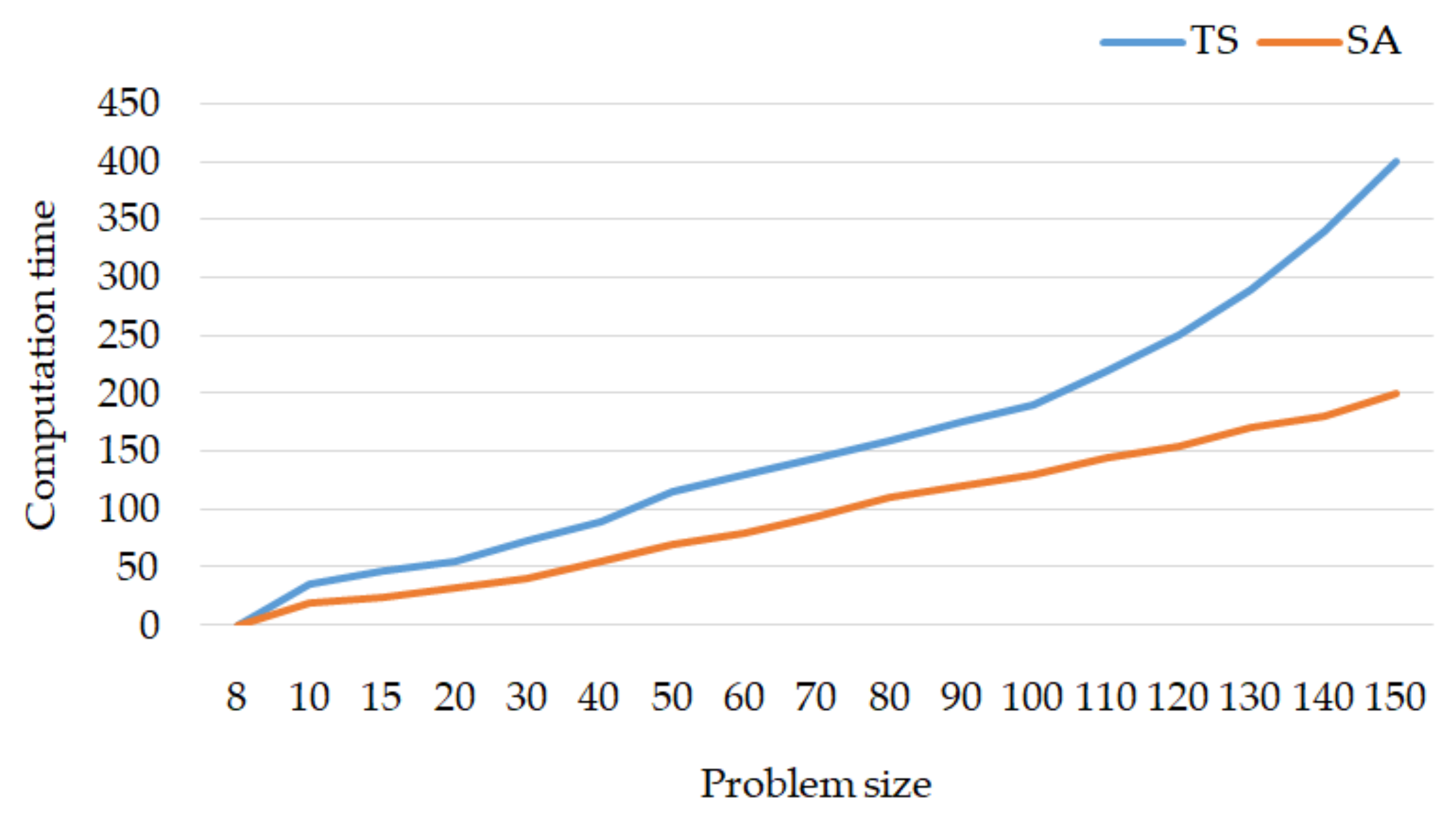
A comparison between TS and SA is also conducted for complex problem instances and respective results are provided in Figure 2. Each problem instance was executed 10 times. For smaller instances (PS < 50), there are not any large-scale computation differences between TS and SA. However, as the problem size crosses a certain limit (PS > 70), there is an evident shift between the curves. SA proves to be more computationally robust compared to TS, as much as, when the problem size is 150, SA takes almost half the time taken by TS in solving the problem. These findings agree with the earlier reported results (Table 9).

The values of the average percent relative deviation for different problem instances are provided in

Table 10. Results of problem instances of SA and TS in comparison to LB.

Algorithm	Problem Set	<PRD> %	Algorithm	Problem Set	<PRD> %
SA	1	1.8	TS	1	2.1
	2	2.4		2	2.7
	3	2.9		3	3.5
	4	3.5		4	4.0
	5	3.9		5	4.7
	6	4.4		6	5.3
	7	4.7		7	5.8
	8	5.3		8	6.3
	9	5.8		9	6.8
	10	6.7		10	7.5

. These values were taken as an average of PRD values of different iterations. It should be noted that the gap between the optimal solution and lower bound value is 1.65%. The maximum (minimum) values of <PRD> for SA and TS are respectively 6.7% (1.8%) and 7.5% (2.1%). The overall average <PRD> values for SA and TS are respectively, 4.14% and 4.87%. Also, the mean gap value for SA is 2.49% (4.14–1.65%) while it is equal to 3.22% (4.87–1.65%) for TS. It can be concluded that, in the presence of LB, SA outperforms TS in terms of maximum, minimum, and average <PRD> values as well as in terms of mean gap value.

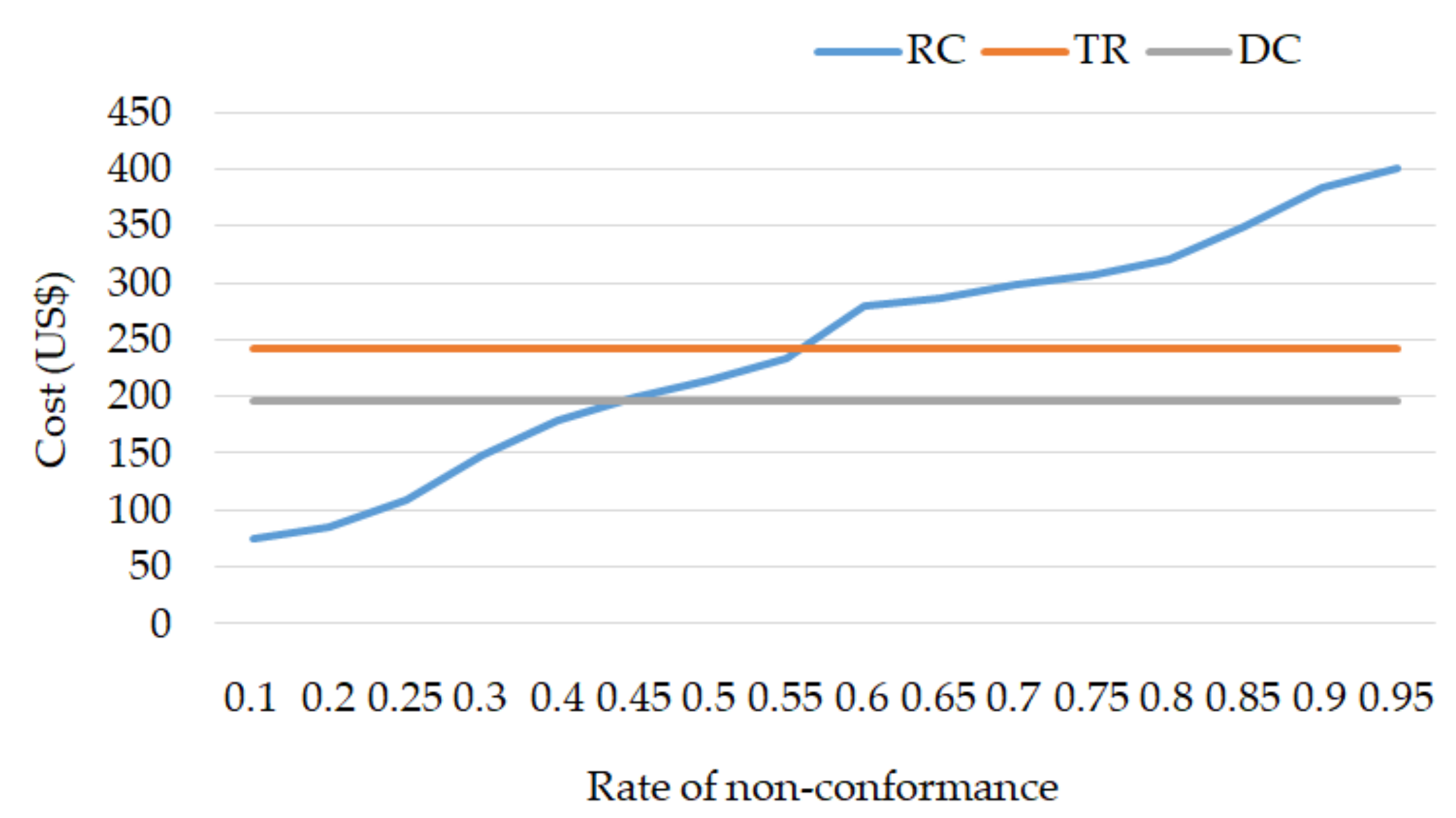
A non-conformance rate is used in the proposed model to consider the quantity of returning goods. Figure 3 contains the results of 3 cost factors for different non-conforming rates. The horizontal axis provides different rates of non-conformance (0.1–0.95) and the vertical axis contains the cost values associated with these rates. The horizontal lines represent the cost of docking (DC) and transportation routes (TR) for a forward flow. It can be observed that these routes are not affected by changes in non-conformance. However, the blue line which provides the cost of returned goods for different non-conforming rates is increasing non-linearly. It is evident that, with an increase in the rate of non-conformance, the cost of return route also increases. For instance, when the rate of non-conformance increases from 0.1 to 0.95, the associated cost increases by more than 300%.

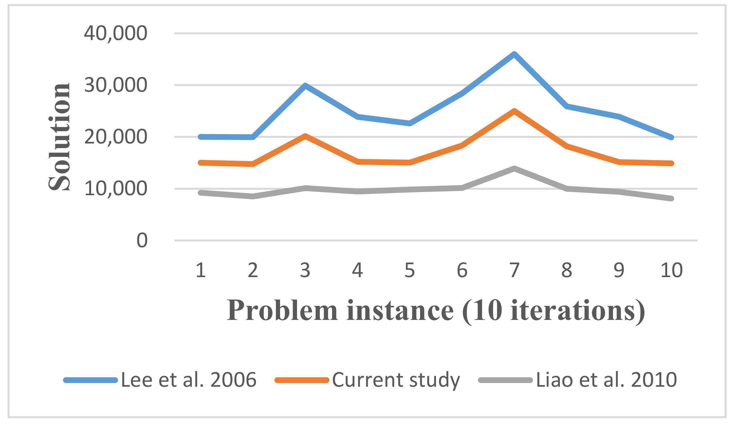
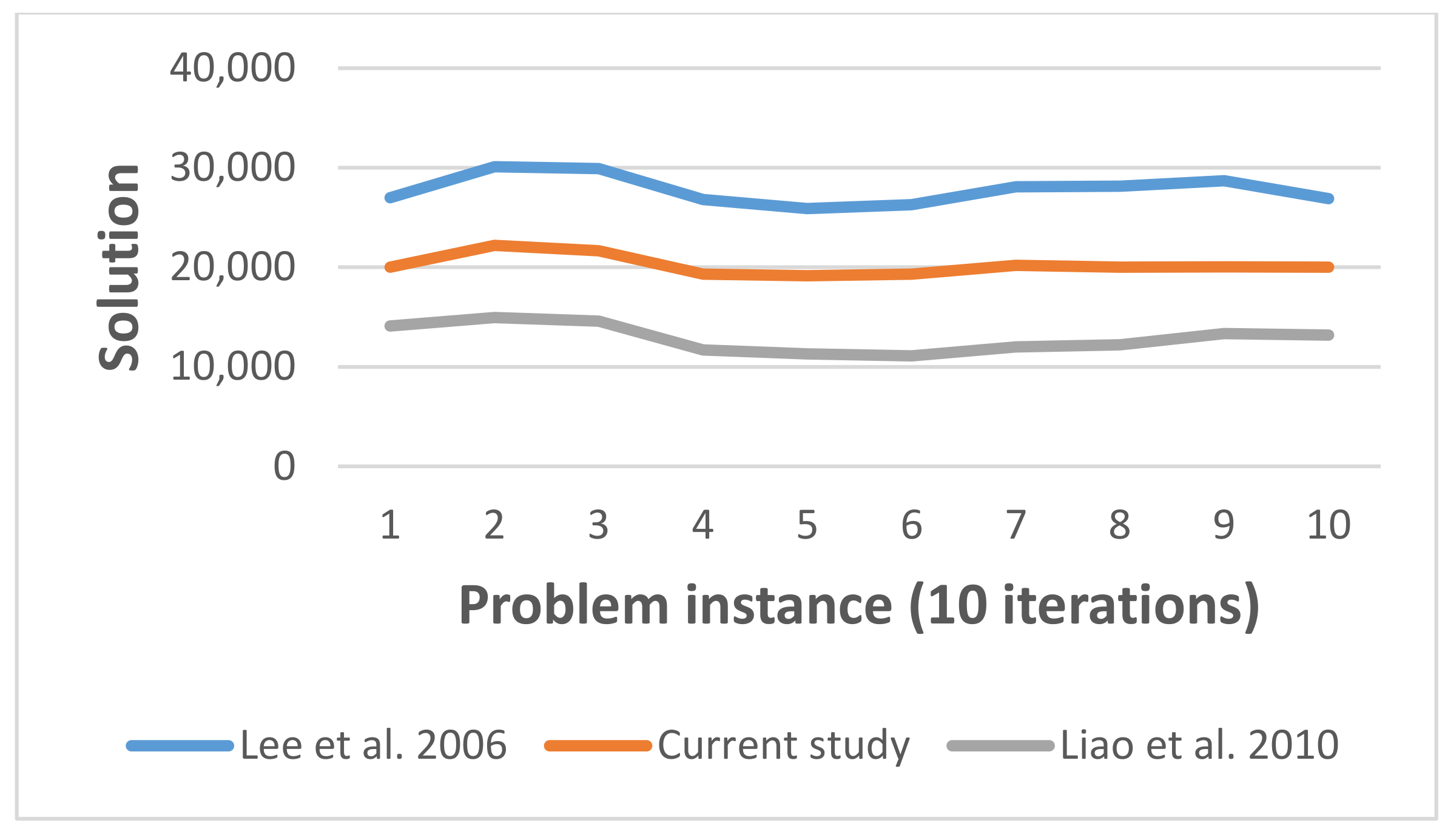
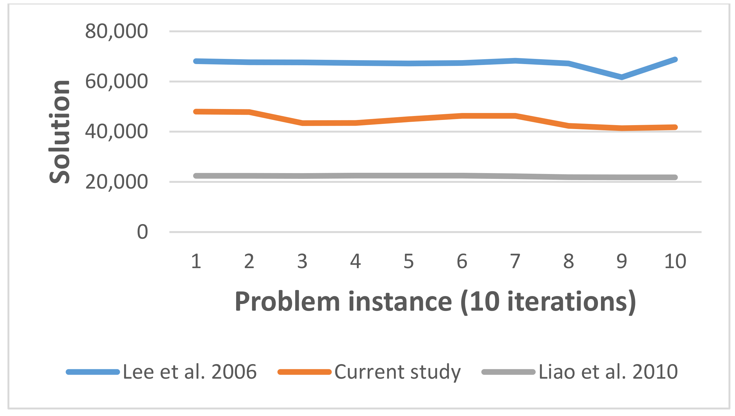
Several other test runs were performed using tabu search. A comparison was made between the findings of the current study and benchmark analysis. The findings of these comparisons are provided in Figure 4, Figure 5 and Figure 6. The horizontal axis of each figure provides 10 randomly selected instances of the NP-hard problem while the vertical axis provides the solutions. Each instance of the problem was executed 10 times to gain statistical confidence.

Several observations can be made from these illustrations. First, by increasing the number of iterations, the deviation in the results of different instances is minimized. In other words, the curves become flatter as the number of iterations increases. Secondly, the results obtained using our approach are somewhat better than those obtained in Lee et al. [74] but are inadequate than the results reported by Liao et al. [65]. The current study results can be taken as a trade-off measure of the established results in literature.

A comparison is also offered to examine the robustness of SA solution approach. A comparison of obtained results is presented with the benchmark findings [34] by considering two problem sizes. These problem sizes are obtained by multiplying the number of transportations, cross-dock, delivery nodes, and the fleet of vehicles. The problem sizes of 5 × 10 × 30 × 2 and 5 × 15 × 30 × 3 is used. Five annealing cooling rates have been considered within each problem size, i.e., 0.20, 0.45, 0.65, 0.85, and 0.95.

The findings are provided in

Table 11. Comparison of SA based obtained results with Jayaraman et al. [34].

Size	Cooling Rate	Jayaraman et al. [34]	Current Findings
5 × 10 × 30 × 2	0.20	0.016	0.018
	0.45	0.026	0.029
	0.65	0.048	0.049
	0.85	0.132	0.123
	0.95	0.376	0.354
5 × 15 × 30 × 3	0.20	0.022	0.025
	0.45	0.030	0.037
	0.65	0.066	0.069
	0.85	0.158	0.153
	0.95	0.498	0.487

. The results obtained in [34] for small cooling rates are computationally more efficient than our findings, however, for advanced cooling rates (0.85 and 0.95), the current results are attained in relatively less computation time. In other words, the obtained results are more robust when there is a drop in annealing temperature. For assessment of GHG emissions, an estimate can be established considering the distance-based formulation from DEFRA (2019) [76]:

GHG emissions = total distance in km × fuel per km × fuel conversion factor

DEFRA takes the relative CO₂/km performance of the European Environment Agency (EEA) CO₂ monitoring database source as the payload capacity information. For the present study, a fuel conversion factor of 2.687 kg/l for diesel is taken from the DEFRA report (2019) [76]. For the presented model, the meta-heuristic simulations predicted an average fuel cost of US$250 between node i and j under the assumption that all trucks have the same engine capacity other dynamic performance parameters. By assuming a fixed price of diesel (1 L = $US1.4) and taking an average distance of 12 km per liter for standard 3.5-ton light vehicle goods, the estimated environmental emissions are:

In

Table 12. Estimated guideline for GHG emissions.

Total Distance (km)	Fuel per km	Fuel Conversion Factor [76]
250 × 1.4	1.4/12	kg CO2e	kg CH4	kg N2O
2160	0.11667	2.68697	0.00030	0.03425
Model based predicted GHG Emissions per km
	kg CO2e	kg CH4	kg N2O	Total (kg)
	0.31348	0.00004	0.00400	0.31751
DEFRA, Table 19 [75], GHG emissions per km for 3.5-t Goods Transportation Vans
	0.26400	0.00001	0.00185	0.26200
% difference (Simulation predicted values—DEFRA estimated values)
	4.95	0.00	0.21	5.55

, a comparison of the predicted GHG emission per km and the DEFRA established emissions show a good corroboration. The percent difference between the predicted and actual established total emissions is found to be 5.55, which indicates the conformance of the mathematical model and meta-heuristic studies. Overall, the proposed methodology presents a good guideline for determining an optimal solution for sustainable vehicle routing problems considering the economic and environmental impacts.

6.1. Sensitivity Analysis

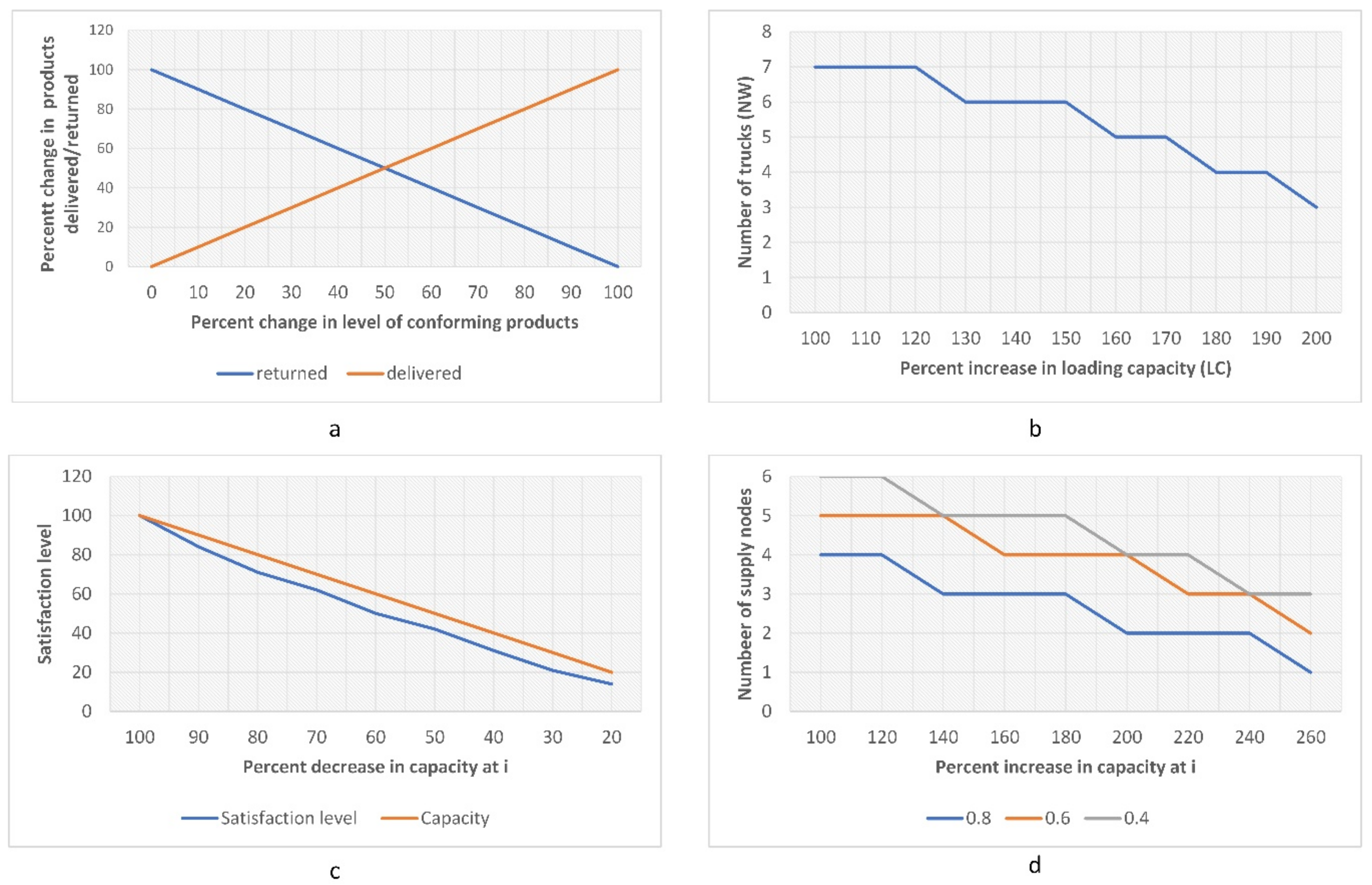
The presented model is based on CLSC network design in the presence of product non-conformance subject to capacity and loading constraints. This sub-section offers an insight into the effect of different model parameters on the sensitivity of various decision aspects of a CLSC network. Figure 7a–d presents the results of sensitivity analysis of various performance indices of the network. Figure 7a shows the impact of an increase in the level of conformance (α) on the number of delivered/returned products. When α = 0, it means that all transported products are failed during the transit. Such failure can be attributed to reasons such as imperfect refrigeration and road conditions etc. Thus, all products are returned, and none are delivered. As the level of conformance increases, the quantity of conforming products delivered increases and the returned products level diminishes. A trade-off is beneficial for managers to balance the quantity of delivered and returned products.

A homogeneous fleet of trucks was used in the CLSC network design. It is imperative to examine how the model reacts towards changes in the capacity of trucks. In this regard, Figure 7b presents a relationship between a percent increase in the truck capacity on the number of trucks used. The 100% LC refers to the initial truck capacity. It can be observed that a straightforward relationship between these two aspects does not exist, rather a reduction in the number of trucks occurs after a certain level of increase in the loading capacity of trucks. Under the current circumstances, it is not feasible to increase the loading capacity of trucks from 100%, 130%, 160% and 180% to 120%, 150%, 170% and 190%, respectively as it will not help in reducing the number of trucks. Thus, although managers may invest in bigger trucks in certain cases, such decisions may not payback and are non-viable. A viable option will be to increase the loading capacity from 120%, 150%, 170% and 190% to 130%, 160%, 180% and 200%, respectively. In these cases, the number of vehicles can be reduced while meeting the required level of demand.

The satisfaction of customers is an integral part of an efficient supply chain network design. It can be measured in terms of high-quality delivery, and responsiveness, etc. It can also be measured in terms of the level of products delivered to customers. To demonstrate this aspect, constraints (7) and (12) were relaxed so that the demand and truck capacity constraints are omitted. Following this, initially, the number of available supply nodes was restricted to 4, i.e., I = 4. A comparison was drawn between the capacity levels at node i and the customer satisfaction i.e., the number of products delivered. Figure 7c provides the relationship between the decrease in capacity at node i and the percent change in customer satisfaction. It is worth noticing that the data point of 100% on either axis refers to the baseline data when the constraints are not relaxed. It can be observed that as the capacity level at the nodes decreases, customer satisfaction decreases at a faster rate. It is because that portion of the transported products are non-conforming and are returned. Thus, not all the units at supply node i are delivered and hence a relatively sharp decline in customer satisfaction is observed. Thus, the level of conformance and non-conformance affects customer satisfaction. To further investigate this aspect, the model was re-run by using three different values i.e., 0.8, 0.6, and 0.4. The relevant results are provided in Figure 7d. The main difference between the analysis in Figure 7c and d is that the latter is based on demand fulfilment constraints. The results indicate that a reduction in the number of supply nodes is observed as the capacity at node i increases. Further, a higher number of supply nodes are needed when the rate of conformance decreases. This is logical because a lower conformance means that a higher quantity is returned, and thus more product units are to be sent to meet the level of demand at the destination. Hence, a higher number of supply nodes will be needed to accommodate such higher product quantities in the presence of capacity constraints.

6.2. Managerial Implications

The CLSC network designs have offered an opportunity for practitioners to reduce the carbon footprints and retrieve products back from the customers. This study offers the following guidelines for managers and practitioners working in the relevant industry. In the presence of higher non-conformance, the return route cost increases. Thus, either the conformance of products is to be ensured by using high quality products through adequate refrigeration or the return route is to be properly designed. One way to do this is by opening a refurbishing plant close to the customer locations so that the return distance can be reduced.

Managers are always interested in reducing the overall cost of the network. It can be reduced by using a limited number of trucks by expanding the loading capacity of trucks. However, the current findings inform that not all expansion decisions are viable, as in some cases, minor expansion in capacity does not reduce the number of trucks. This will offer an opportunity for managers in deciding when and to what extent an investment decision in larger trucks should be made. Lastly, a relationship was established between the capacity at the supply node and customer satisfaction. In some cases, higher capacity levels may be needed to ensure higher customer satisfaction.

7. Conclusions

This study analyzed a CLSCCD problem for optimizing the objective of cost which comprised of costs related to production, transportation, handling, penalty, and the cost of the product return. Two flow types, i.e., forward and return flows were considered as part of the analysis by considering the non-conformance of products. A mathematical model and two heuristic approaches were adapted to analyze the problem. The branch-and-bound method was used for small problem instances whereas meta-heuristics were used for higher-order problem sizes. The analysis was presented by using parameter tuning, benchmark experiments, and a lower bound approach. A comparison between Tabu search and Simulated Annealing proved that the latter was a computationally efficient and robust measurement approach due to an initial heuristic embedded with it for refining the solutions.

A higher rate of conformance of product delivery can enhance customer satisfaction. It can be ensured by employing perfect refrigeration conditions and monitoring the road conditions. Similarly, attention needs to be paid to the capacity expansion of trucks and its impact on the number of trucks used. Not all expansion decisions are viable in reducing the number of trucks. However, it is pertinent to reduce the number of trucks in transit to reduce emissions.

Since an indirect measure was used to analyze the product quality, therefore, there is a dearth of using a direct measure to capture the quality of products during transit. Future research can define a dedicated objective function that defines the quality of in-transit products subject to imperfect refrigeration. This study made assumptions regarding the traveling distance, the capacity of trucks, fuel efficiency, and environmental impacts. It was assumed that the unit distance cost is the same for all routes, loading capacity is same for all trucks as well as for all nodes. Future research can relax these assumptions by considering variable distance cost and variable capacity of a truck for different routes. The presented model was deterministic with respect to the behavior of different aspects of the analysis. It will be interesting to formulate a robust variant of this model by considering stochastic aspects. Such practice will help in comparing the deterministic and stochastic behavior of various input parameters to consider a more informed decision. The initial heuristic embedded SA outperformed the Tabu search approach. Future research may embed an initial heuristic with Tabu search to understand how well it performs subject to modifications. Similarly, the discussion can be extended by comparing the results of meta-heuristics with other methods, such as genetic algorithms and the Petri-net approach.

The proposed modeling and simulation approach can be used for strategic and operational decisions in the supply chain, for instance, designing the sustainable network configuration, resource management, and optimal routing to reduce the GHG emissions. The mathematical model and meta-heuristic algorithms can be extended by incorporating other complicated objectives simultaneously, such as vehicle fuel efficiency parameters, traffic condition of a road network, and availability of alternate vehicles.